Abstract
Landslides recurrently cause severe damage and, in some cases, the full disruption of many highways in mountainous areas, which can last from a few days to even months. Thus, there is a high demand for monitoring tools and precipitation data to support highway alignment selections before construction. In this study, we proposed a new system highway alignment selection method based on coherent scatter InSAR (CSI) and ~1 km high-spatial-resolution precipitation (HSRP) analysis. Prior to the CSI, we calculated and analyzed the feasibility of Sentinel-1A ascending and descending data. To illustrate the performance of the CSI, CSI and SBAS–InSAR were both utilized to monitor 80 slow-moving landslides, which were identified by optical remote-sensing interpretation and field investigation, along the Barkam–Kangting Highway Corridor (BKHC) in southwestern China, relying on 56 Sentinel-1A descending images from September 2019 to September 2021. The results reveal that CSI has clearer deformation signals and more measurement points (MPs) than SBAS-InSAR. And the maximum cumulative displacements and rates of the landslides reach −75 mm and −64 mm/year within the monitoring period (CSI results), respectively. Furthermore, the rates of the landslides near the Jinchuan River are higher than those of the landslides far from the river. Subsequently, to optimize the highway alignment selection, we analyzed the spatiotemporal evolution characteristics of feature points on a typical landslide by combining the −1 km HSRP, which was calculated from the 30′ Climatic Research Unit (CRU) time-series datasets, with the climatology datasets of WorldClim using delta spatial downscaling. The analysis shows that the sliding rates of landslides augment from the back edge to the tongue because of fluvial erosion and that accelerated sliding is highly related to the intense precipitation between April and September each year (ASP). Consequently, three solution types were established in our method by setting thresholds for the deformation rates and ASPs of every landslide. Afterward, the risk-optimal alignment selection of the BKHC was finalized according to the solution types and consideration of the construction’s possible impacts. Ultimately, the major problems and challenges for our method were discussed, and conclusions were given.
1. Introduction
Throughout history, reliable road networks have been vital local assets, connecting communities and unlocking economic growth [1,2]. Since China’s Belt and Road (B&R) policy was proposed in 2013, the complexities of trade and cultural exchange have led to a steady growth in highway volume, especially in mountainous areas of southwestern China. Their good condition and safety have become paramount concerns to cater to socioeconomic development. However, landslides in the highway corridor are the most common hazardous and recurrently appearing natural disasters, which can be triggered by intensive rainfall, earthquakes, fluvial erosion, geomorphological processes, and human activities [3,4,5,6,7,8,9,10,11,12,13]. In general, the most direct solution to avoid landslides is risk-optimal alignment selection, which highlights the value for effective monitoring and HSRP analysis.
Among the variety of remote-sensing techniques in the last decade, time-series interferometric synthetic aperture radar (TS–InSAR) has been widely applied to accurately quantify ongoing landslide movements. It was developed to overcome temporal and geometrical decorrelations and atmospheric delay anomalies by focusing on coherent radar targets instead of the ensemble of image pixels [14,15,16,17,18,19,20]. According to the scattering mechanisms of the ground target, there are two main categories: persistent scatter (PS) and distributed scatter (DS). PS methods focus on point-like coherent targets, which have a highly stable backscattering behavior, such as artificial reflectors, bare rocks, or manmade structures. Only a single master image is selected; consequently, N − 1 interferograms are produced from N single-look complex (SLC) SAR images after co-registering to the master in PS methods. The PSInSARTM, IPTA, StaMPS/PSInSAR, SPINUA, STUN, SPN, and PSP algorithms are representative PS methods [15,16,17,21,22,23,24,25,26,27,28]. Contrariwise, DS approaches utilize distributed targets, such as bare soil and sparsely vegetated or desert lands, which contain many small random scatters. In DS methods, M(N − 1 < M < N(N − 1)/2) multi-master interferograms with short spatiotemporal baselines are generated. SBAS, QPS, and TCPInSAR are the main DS algorithms [14,19,25,26,27,28,29]. To maximize the spatial sampling of deformation signals over rural regions, multi-temporal InSAR (MTInSAR) and SqueeSARTM have been proposed as next-generation time-series InSAR techniques [16,17,18,19,20,21,22,23,24,25,26,27,28,29,30,31,32,33,34]. Particularly, both PS and DS targets are processed to obtain deformation signals in SqueeSARTM. The evolution of the SqueeSARTM, including JSInSAR, CAESAR, PD–PSInSAR, GEOS–ATSA, and CSI, has made TS–InSAR the fundamental tool in landslide monitoring [35,36,37,38,39,40,41,42]. Thus, hundreds of InSAR-related papers for landslide studies have been published per year [1,5,6,8,9,10,11,12,13,14,15,16,17,18,19,20,21,22,23,24,25,26,27,28,29,30,31,32,33,34,35,36,37,38,39,40,41,42,43,44,45,46,47,48,49,50,51,52], which accelerate the comprehensive development of space–air–ground landslide investigation systems. The most worthy of mention are the differences in CSI and SqueeSARTM: first, CSI adopts the generalized likelihood ratio (GLR) test as an alternative to the Kolmogorov–Smirnov (KS) test for statistically homogeneous pixel (SHP) identification if the number of available SAR images is less than 20; second, CSI uses a phase-linking approach to estimate the optimal interferometric phase values from the complex coherence matrix for each DS target; third, both PS and DS scatters are combined to create the Delaunay triangular network for phase unwrapping, and the deformation is estimated using standard time-series analysis procedures; fourth, CSI significantly increases the spatial density of MPs and, thus, makes phase unwrapping robust [42].
However, in mountainous areas, no matter which algorithm is utilized, geometric distortions, such as foreshortening, layovers, and shadows, will lead to lower monitoring resolution and precision of target landslides, even missing observations. Hence, besides these algorithms, monitoring accuracy is mostly determined by the feasibility of SAR data (FS). And sometimes, there is no need to utilize both ascending and descending SAR data because tremendous data redundancy will reduce the TS–InSAR’s efficiency, especially in wide ranges. Under this circumstance, some researchers have proposed methods to analyze the geometric distortion of SAR data and calculate the FS based on DEM and satellite orbital parameters [43,44,45,46,47].
According to statistics, landslides caused by rainfall account for approximately 70% of the total number of landslides, and 95% of these occur in the rainy season. Thus, HSRP data are essential for related phenomena that affect hydrology, vegetation cover, and geohazards. Although meteorological observation networks are increasingly incorporating data from a large number of weather stations and contributions from an increasing number of governments and researchers around the world, observation networks still suffer from low station density and spatial resolution in mountainous regions [53]. Thus, several interpolation methods, such as inverse distance weighting, kriging methods, and regression analysis, are used to generate meteorological data for ungauged areas. However, the station density decides the result accuracy of these methods [53,54,55,56,57,58,59]. In general, precipitation data products are released by several climate research organizations, including general circulation models (GCMs), the Climatic Research Unit (CRU), the Global Precipitation Climatology Centre (GPCC), and Willmott and Matsuura (W&M) [60,61,62]. Particularly, CRU products include the monthly mean precipitation, which is generated from data obtained from observational stations but has a low spatial resolution (~55 km). Nevertheless, the climate changes drastically per kilometer in the mountainous areas of southwestern China, especially the precipitation, which induces landslide instability. In practice, the ~1 km HSRP needs to be combined with the results of the TS–InSAR to optimize the highway alignment selection. Consequently, it is necessary to spatially downscale and correct CRU monthly mean precipitation products. Previous studies have proved that the delta downscaling framework is suitable for monthly precipitation data downscaling using CRU products [60,63,64,65,66].
Field investigation and optical remote-sensing interpretation are employed in the conventional highway alignment selection method; sometimes, drilling wells are needed too. The drawback of this method is the high human and economic costs. As a major traffic connection to the Bangladesh–China–India–Myanmar International Economic Corridor and the Silk Road Economic Belt in the Tibetan area of Sichuan Province, the alignment selection problem of the BKHC is severe because of the complicated geological background, strong tectonic movement, rock body rupture, as well as frequent geohazards. To solve the problem of the conventional method, in this paper, we propose a new systematic highway alignment selection method based on CSI and ~1 km monthly HSRP analysis.
First, the FSs of the Sentinel-1A ascending and descending data were calculated. Consequently, based on 56 Sentinel-1A satellite images from September 2019 to September 2021 (before the design was finalized), both CSI and SBAS-InSAR were utilized in a typical section of the BKHC (from Jinchuan to Danba), which has 80 slow-moving landslides identified by optical remote-sensing interpretation and field investigation. The comparison results of the two methods illustrate that CSI has better performance. Subsequently, three solution types were established in our method by setting thresholds for deformation rates (CSI results) and ASPMPs of every landslide. Finally, the risk-optimal alignment selection of the BKHC was finalized according to the solution types and consideration of the construction’s possible impacts.
2. Study Area and Data Sources
2.1. Study Area
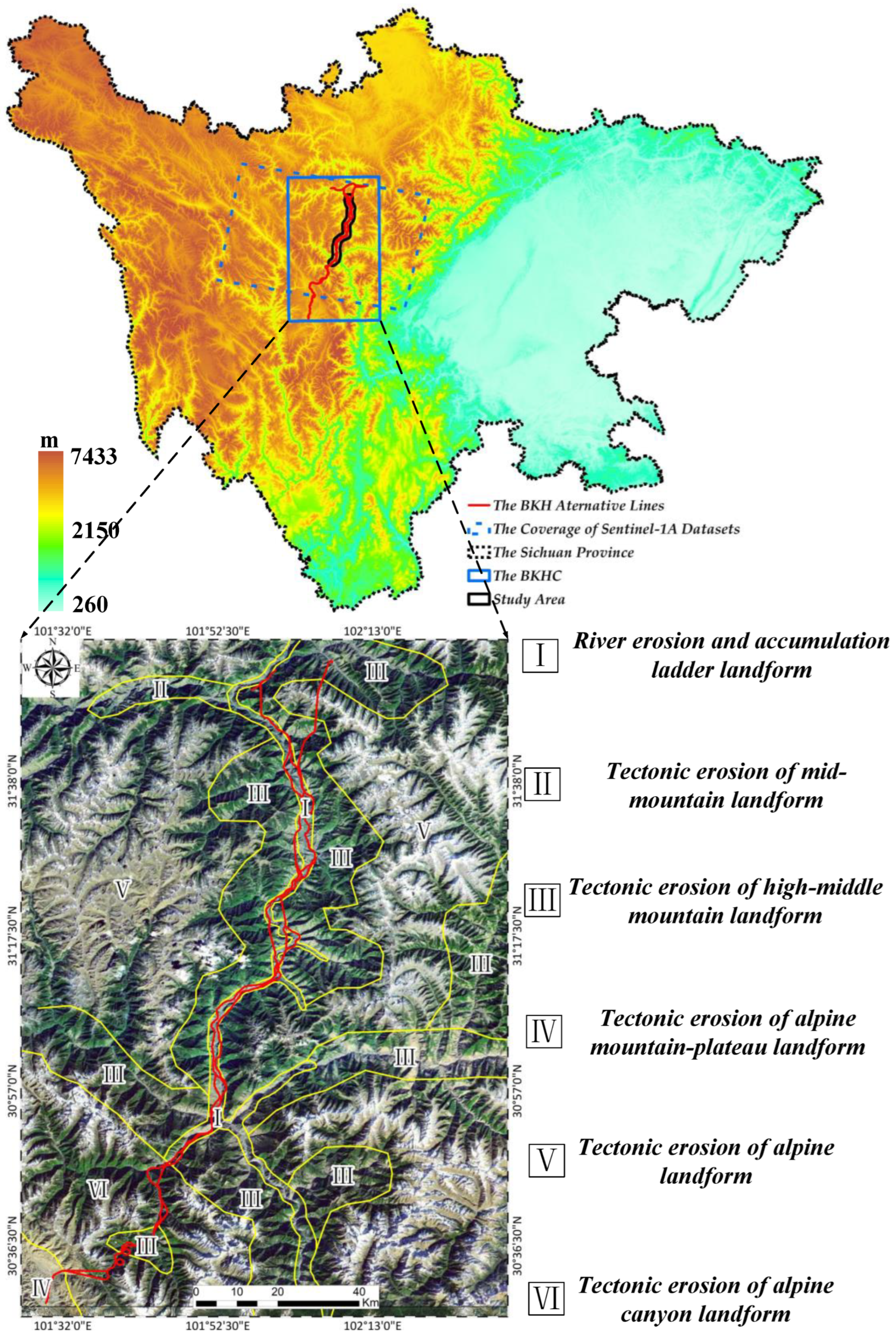
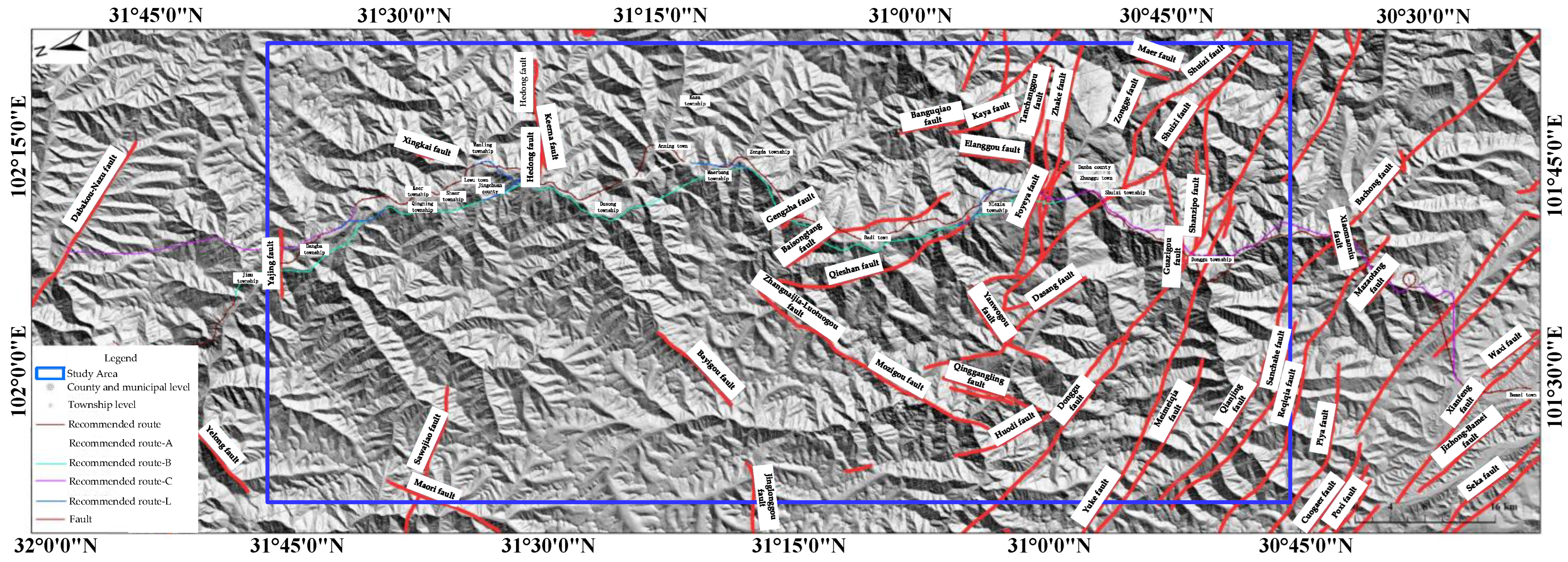
As depicted in Figure 1, the BKHC goes from northeast to southwest, accompanied by the G248 national highway. This corridor is located in the cascade zone between the Qinghai–Tibet Plateau and Sichuan Basin, which goes through the tectonic erosion of the high–middle mountain landform, tectonic erosion of the alpine landform, river erosion and accumulation ladder landform, tectonic erosion of the alpine canyon landform, and tectonic erosion of the alpine mountain–plateau landform. Topographically, the BKHC is characterized by deep valleys and rugged mountains, with elevations ranging from 1800 m to 5300 m. As depicted in Figure 2, more than 18 active faults intersect the route’s lines. Strong tectonic movements have produced deep, narrow river valleys. Meanwhile, the rainy period in this region usually lasts from April to September. The monthly precipitation in this period far exceeds that in any other months. The complex geological, hydrological, and geotechnical processes provide dynamic conditions, which promote the occurrence of landslides.

Figure 1.
Overview of the study area.
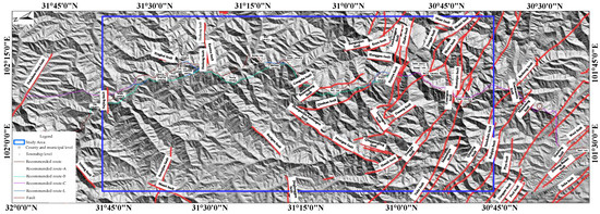
Figure 2.
Faults in the study area.
Along this highway corridor, a typical section from Jinchuan to Danba lies on the river scouring and accumulation ladder landform. Generally, such landforms consist of shorter cliffs and steep slopes. With the river scouring and precipitation, the stability of the vertical sliding surfaces and rock-layer structure becomes weak. Consequently, fully developed landslides are distributed along this section. A 10 km buffer has been taken along this section as the study area.
2.2. SAR Data Sources
A set of 56 descending Sentinel-1A images (from September 2019 to September 2021) and corresponding precise orbit datasets (POD) are provided by the European Space Agency (ESA) (Table 1). In addition, the 30 m resolution digital elevation model (DEM) provided by the National Aeronautics and Space Administration (NASA) is employed to estimate and remove the topographic phase. The coverage of the SAR images is shown in Figure 1 with the blue-dashed box.

Table 1.
Sentinel-1A datasets and primary image parameters.
2.3. CRU and WorldClim Datasets
CRU TS v. 4.07 (https://crudata.uea.ac.uk/cru/data/hrg/cru_ts_4.07/, accessed on 1 April 2023) and WorldClim v. 2.1 (https://worldclim.org/data/monthlywth.html, accessed on 1 April 2023) are used for delta downscaling to obtain the monthly HSRP (Figure 3) [65,66].
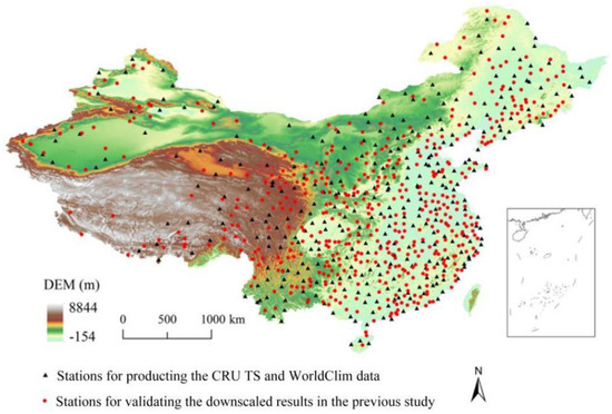
Figure 3.
Distribution of national weather stations across China (modified from Figure 1 from in [62]).
As previous studies have proven, CRU datasets exhibit better performance than other similar gridded products. In addition, 323 weather stations across China were employed by the CRU group to generate CRU time-series data (Figure 3) [63,64,65,66]. And reference WorldClim datasets comprised monthly mean precipitations at 2 m, which were generated based on 9000–60,000 weather stations located globally using the thin-plate spline interpolation method. Remarkably, cross-validation correlations indicated that these datasets exhibited good performance globally because of the introduction of the satellite-derived covariates and distance to the nearest coastal covariates and reflected orographic effects well.
3. Methods
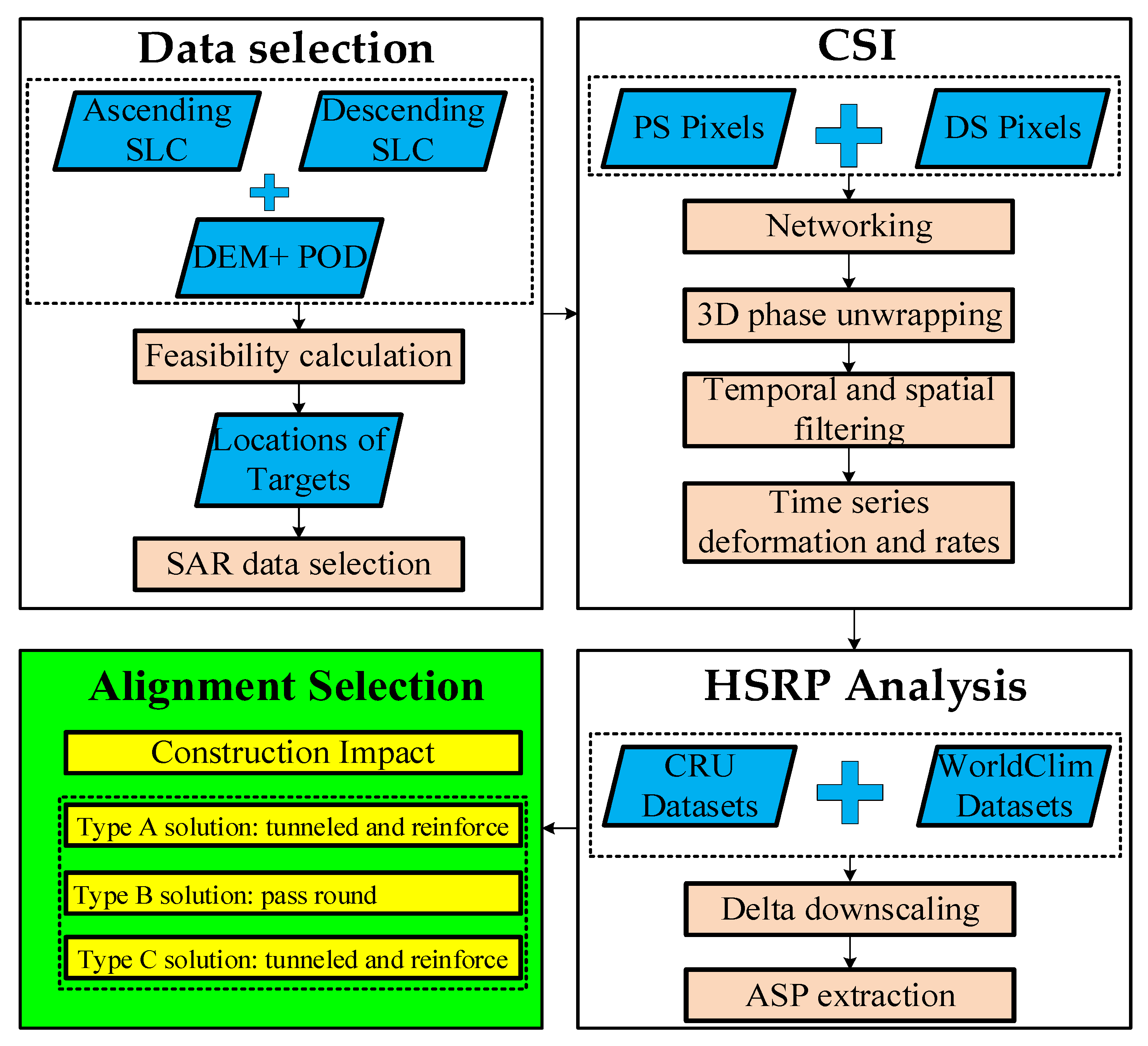
In this paper, we propose a new systematic highway alignment selection method to finalize the landslide-hazard-avoiding highway alignment of the BKHC, which consists of four steps, i.e., data selection (feasibility calculation of SAR data), CSI and monthly HSRP analysis, and alignment selection (based on the locations, three solution types, and the construction’s possible impacts, as depicted in Figure 4). Each of the four steps will be illustrated in detail.

Figure 4.
Method flow.
3.1. Data Selection
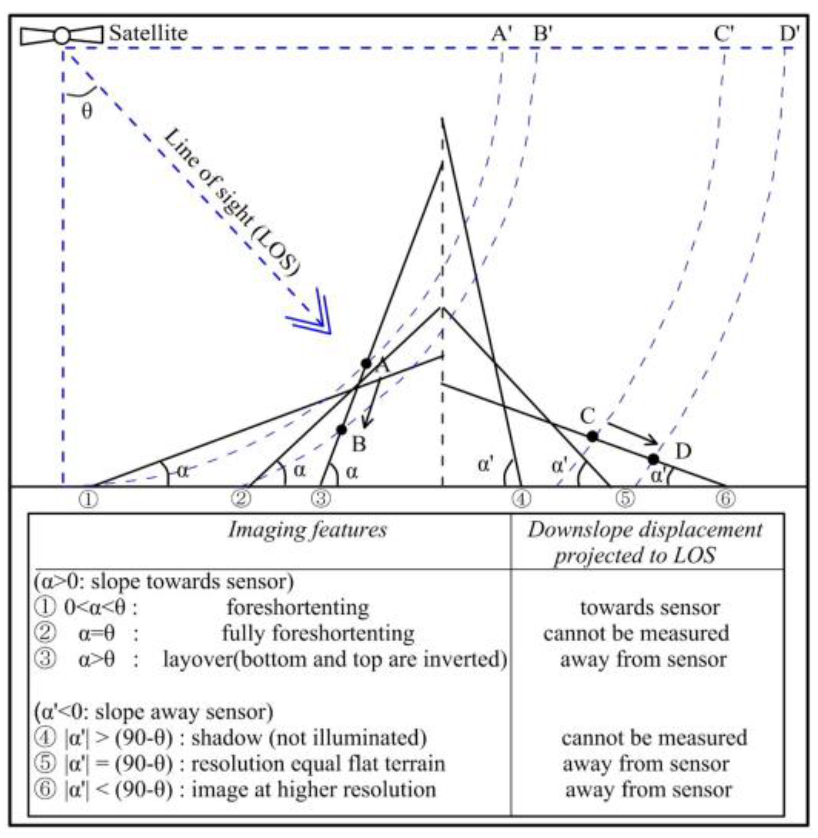
The relationships between the line of sight (LOS) and slope displacements are summarized in Figure 5 [67]. The slope orientations and features, which are reflected in the DEM, determine the geometric distortion occurrence. The feasibility of the SAR data (FS) is calculated based on the DEM (slope angles and aspects) and the satellite orbit parameters (slant range) [68]. Generally, the shadow effect occurs when the beam cannot illuminate a parcel of terrain because of a physical barrier. Likewise, the layover effect indicates the pixels affected by distortion occurring when the front of the radar beam reaches the top of a slope before it reaches its base. And both shadow and layover effects are more likely to occur in far ranges and on slopes facing the same direction as the beam or in near ranges for small incidence angles. Herein, we take the local incidence angle, which is, namely, the angle between the incident radar beam and a line that is normal to that surface, as a basis calculation factor.
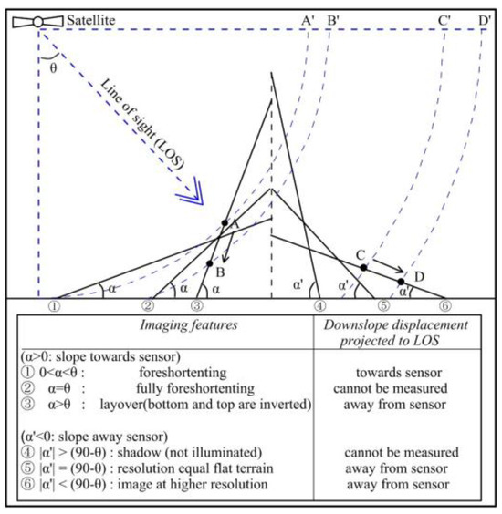
Figure 5.
Relationship between the LOS and the downslope displacements for different slope orientations (scenarios 1, 2, and 3 are facing the sensor and scenarios 4, 5, and 6 are facing away from the sensor) and slopes (α and α’) (adapted with permission from Ref. [67]. 2016, Keren Dai).
Hence, the FS can be calculated using Equation (1) [68]; all the calculation factors must be in radians. The slope and aspect can be derived using the DEM, and the Flat_area can be extracted by classifying the slope. The Lay_Shad_mask needed a reclassification from the original data, which was created by assigning a value equal to 0 for the pixels affected by the layover and/or shadow and 1 for the others. The local incidence angle was calculated using Equation (2), where denotes the height from the satellite to the center of the Earth, denotes the geodetic height of the sub-satellite point on the Earth, denotes the near slant range, and represents the resolution of the slant range.
The local incidence angle was calculated using Equation (2)
where denotes the height from the satellite to the center of the Earth, denotes the geodetic height of the sub-satellite point on the Earth, denotes the near slant range, and represents the resolution of the slant range.
The FS calculation results are classified into 4 classes according to the effects of the terrain’s geometry (Table 2). The SAR data composition selection can be determined based on these 4 classes [68].
Table 2.
Feasibility of SAR data.
3.2. CSI
As TS–InSAR methods, PS and DS algorithms have been widely used in landslide monitoring. The PS algorithm focuses on the selection of PS targets, while the DS algorithm identifies DS targets and their optimal phases. CSI combines these two targets for further analysis using a standard PSI tool, which can reflect the details of landslide deformations better with enough points [42].
3.2.1. PS Target Selection
As the first generation of the TS–InSAR, the PS algorithm is a mature algorithm that integrates into a variety of commercial or open-source tools. In CSI, StaMPS is employed to select PS points based on amplitude and phase information because of the close relationship between the amplitude stability and phase stability when the coherence is high [42,69]. Hence, the amplitude dispersion index (ADI) can first be used to select PS targets and is calculated using Equation (3) as follows:
where and denote the mean and standard deviation of a series of amplitude values for one pixel, respectively. When the of a certain pixel is under 0.4, it can be considered as a PS target.
Subsequently, the deformation signal will be assumed to be spatially correlated for each PS target, and the temporal coherence () can be calculated using Equation (4) as follows [69]:
where N and denote the number of images and the estimated residual phase noise of ith SLC image, respectively. Certain PS targets will be kept with the original phase values for further time-series analysis when the their values are high enough.
3.2.2. DS Target Selection
DS target selection has two steps, including SHP identification and optimal phase estimation, as follows:
- (1)
- SHP identification
Generally, it is necessary to obtain sufficient and high-temporal-resolution SAR images (at least 2 years of datasets with a 12~48–day revisiting cycle) to help with highway alignment selection, especially in southwestern China, because of the spatiotemporal discorrelation. Thus, a KS test can be used to identify the SHPs, which needs a large number of samples [70]. The sample’s complex coherence matrix can be estimated using Equation (5) as follows:
where N denotes the number of images, represents the pixels in a fixed window ( 25 × 25) centered on pixel x, is the normalized complex scattering vectors, and H indicates a Hermitian transpose. Particularly, only if the number of SHPs with high weights () in window is larger than 20, pixel x can be selected as a DS target in the CSI.
- (2)
- Estimation of the optimal phase
For each pixel, the optimal phase series can be estimated according to the previous section. is set as 0, and the maximum likelihood estimation (MLE) of can be calculated using Equation (6) as follows:
where = [0, , …, ]T, and the symbol “o” denotes the mathematical operator of the Hadamard product between two matrices obtained using Equation (5). Then, a phase-linking approach can be utilized to solve this equation, which can be expressed as a closed form in Equation (7) as follows [71]:
where k is the iteration step.
To evaluate the quality of the estimated optimal phases, the goodness-of-fit index (GF) can be calculated using Equation (8) as follows:
The GF, illustrated as the extension of the temporal coherence, , is the phase value of item (m, n) in the coherence matrix, and and are the estimated optimal phases. Then, those DS targets with high GF values (higher than the predefined threshold) will be selected as the final DS targets.
3.2.3. Combination of PS and DS Targets
PS and DS pixels can be connected to form a Delaunay triangulation network for phase analysis after first dropping the common pixels. Subsequently, the phase is first corrected for the spatially uncorrelated part of the look-angle error. The final time-series deformation and rate can be retrieved after the 3D phase unwrapping and spatiotemporal filtering [69,72]. All these procedures can be implemented in the StaMPS.
3.3. HSRP Analysis
To obtain the monthly ~1 km HSRP datasets, delta downscaling is a well-suited method, including four steps [53]. First, a climatology dataset is constructed for each month based on 30′ CRU and WorldClim time-series data. Second, the 30′ anomaly time-series data are derived for precipitation based on the 30′ CRU time-series data and the constructed precipitation dataset, which can be expressed using Equation (9) as follows:
where are the anomalies for the precipitation, are the absolute precipitation values, is the 30′ climatology for the precipitation, and m and yr correspond to month (from January to December) and year, respectively. Third, the bilinear interpolation method is employed for the 30′ anomaly grids at each time. The 0.5′ spatial resolution datasets (~1 km) will be retrieved to match the WorldClim data. Finally, the high-spatial-resolution anomaly time-series dataset is transformed to an absolute climatic time-series dataset based on the WorldClim data using Equation (10) as follows:
where are the absolute precipitation values at a 0.5′ spatial resolution (~1 km HSRP), denotes anomalies at the 0.5′ spatial resolution for the precipitation, and are climatology datasets from WorldClim at a 0.5′ spatial resolution for the precipitation.
3.4. Alignment Selection
As the final step of our method, all the accurate results above should be considered comprehensively. The annual deformation rate is one of the most direct factors reflecting the activities of landslides. Usually, when the rate’s absolute value is higher than 10 mm/yr, the landslide is considered as an active event [73]. And when the rate’s absolute value is higher than 30 mm/yr, the landslide is considered as a vigorous active event (The annual deformation rate of every landslide’s geometric center point is selected in our method.).
As for the HSRP, because our study area is in a typical Tibetan Plateau monsoon climate zone, which only has a low mean annual rainfall [42], the rainfall intensities in the rainy season will decide the stability of landslides in such areas [74]. Hence, the total precipitation from April to September of every landslide within the monitoring period (ASPMP) was extracted as our judgment factor based on the ~1 km HSRP. Furthermore, for highways at the local scale, the HSRP is close to a normal distribution, and the ASPMP’s mean value (ASPMPM) for all the landslides within the monitoring period has a higher reference price than any others in the statistics.
On these bases, we set three solution types in our method to decide the risk-optimal alignment selection of the highway: A (|rate| > 30 mm/yr and ASPMP > ASPMPM; tunnel and reinforce), B (10 mm/yr < |rate| ≤ 30 mm/yr and ASPMP > ASPMPM; pass around), and C (|rate| ≤ 10 mm/yr and ASPMP < ASPMPM; remain and reinforce).
4. Results and Analysis
As depicted in Section 3, our proposed method was utilized to typically section the BKHC (from Jinchuan to Danba), which has 80 slow-moving landslides identified by optical remote-sensing interpretation and field investigation, based on 56 Sentinel-1A satellite images from September 2019 to September 2021 (before the design was finalized). As a result, the risk-optimal alignment selection of the BKHC was finalized.
4.1. Results of the FS and Data Selection
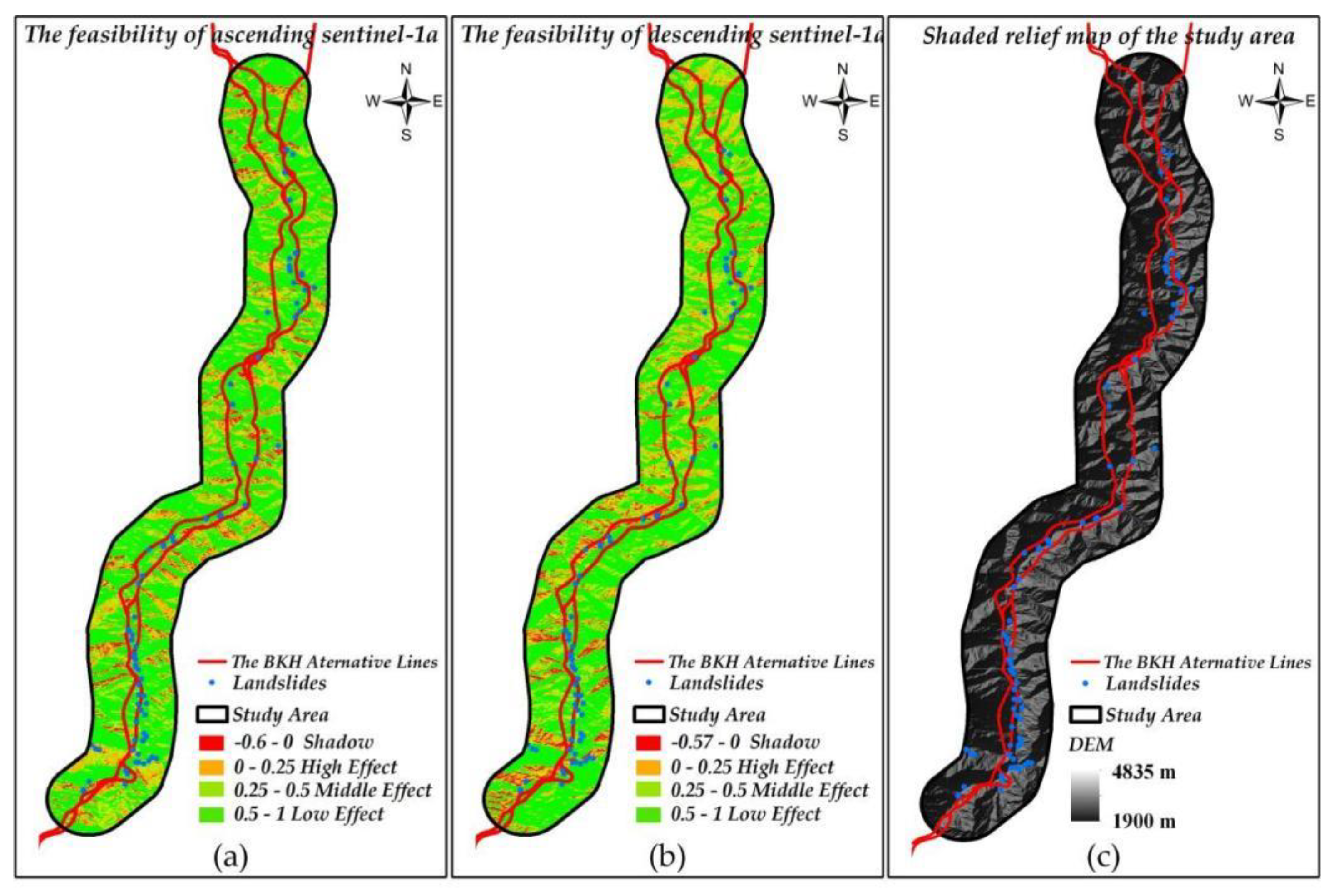
As shown in Figure 6a,b, the FSs of the ascending and descending Sentinel-1A images were calculated. Almost half of these landslides were located in the low-effect area in the descending SAR data, while almost half of them were located in the shadow or high-effect area in the ascending SAR data. Thus, we selected 56 descending images of Sentinel-1A (2019–2021) as the only data source for the CSI. Figure 6c reveals that these landslides are distributed in the river valley; consequently, these landslides have developed well because of the river’s perennial scouring and dense rainfall.
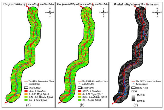
Figure 6.
The FSs of the Sentinel-1A data: (a) ascending and (b) descending; (c) the terrain of the study area.
4.2. Results of CSI and HSRP
To illustrate the improved performance of the CSI, we employed SBAS-InSAR for the same study area based on the same SAR data source [14]. Figure 7a,b shows the annual rates along the LOS direction, as measured using SBAS-InSAR and CSI, respectively. The CSI’s deformation signal and total number of MPs are clearer and higher than those of the SBAS-InSAR, respectively. The maximum annual rate reaches −64 mm/yr within the monitoring period.
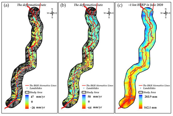
Figure 7.
The LOS deformation rates derived using SBAS-InSAR and CSI: (a) SBAS-InSAR and (b) CSI; (c) ~1 km HSRP in June 2020.
The monthly ~1 km HSRP datasets can be retrieved using the method in Section 3.3; Figure 7c shows an example of the HSRP in June 2020. On this basis, the HSRP and ASPMP of every landslide can extracted one by one.
4.3. Analysis of a Typical Landslide
To demonstrate the applicability of our method to every landslide, we selected the largest landslide as a typical case. This landslide (102.876° E, 30.963° N) is located in Niela Village in Danba County, which is next to the Jinchuan River. The low vegetation coverage makes the interferograms have a high coherence. Meanwhile, the orientation and slope angle satisfy the observations of the descending Sentinel-1A data.
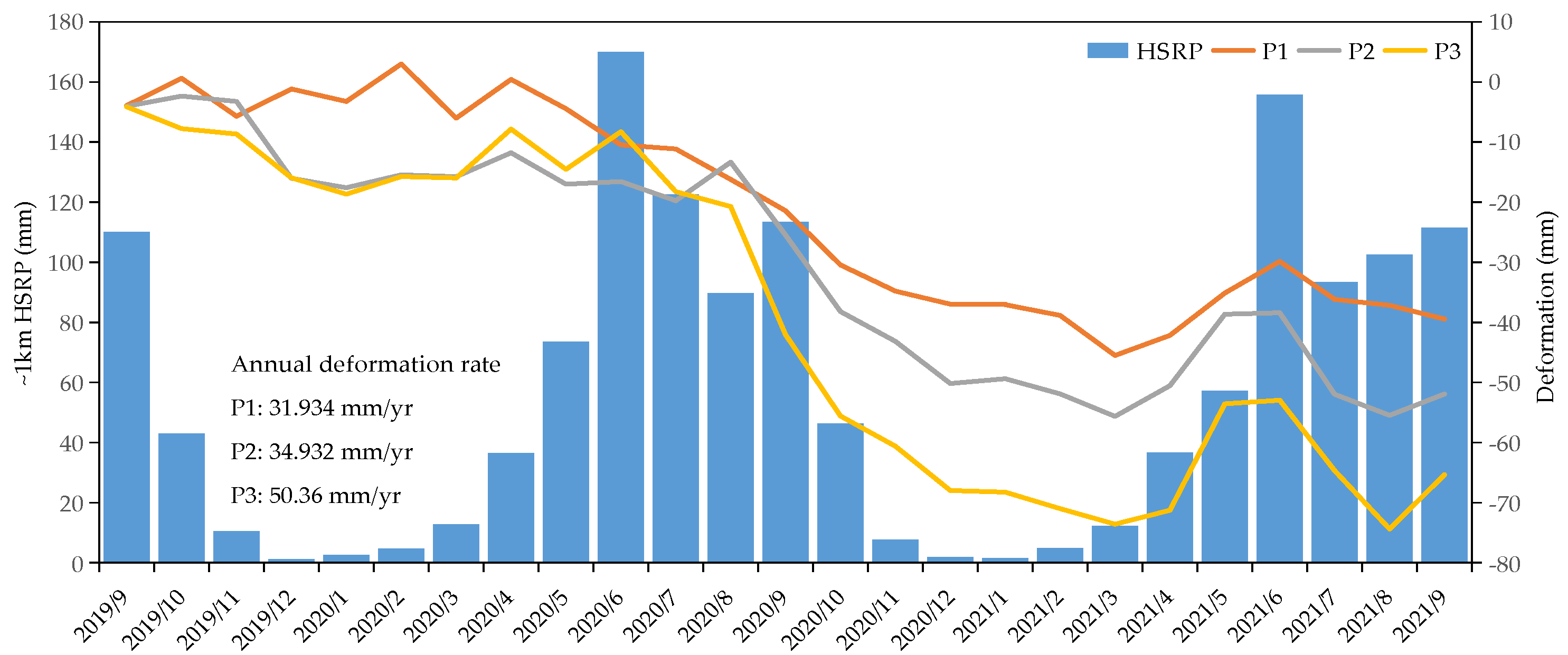
As can be seen from Figure 8, this landslide is about 1150 m long and 1200 m wide, which covers an area of up to 1,275,267 m2. CSI can obtain clearer deformation signals and more MPs than SBAS-InSAR, and the maximum annual deformation’s LOS velocity reached 59 mm/yr. To further reveal the spatiotemporal evolution, the cumulative deformation curve of three points (P1, P2, and P3) from the slope’s back edge to the tongue was combined with the monthly HSRP. To avoid any misunderstanding, we inverted the result’s value to reflect the slip down. As shown in Figure 9, the cumulative displacement in the period of the monitoring reached almost 75 mm, and accelerated sliding is highly related to intense rainfall events between April and September each year (the temporal window for our ASPMP). Therefore, the gathered precipitation may have contributed to the formation of gullies on the landslide body. Water from the gullies infiltrates deposits composed of silty clay, gravelly soil, and cracks; consequently, a slip surface formed. With increasing water content and slope weight, the slip accelerates significantly.
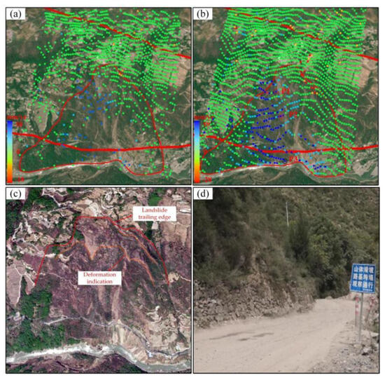
Figure 8.
The annual deformation rates derived from descending Sentinel-1a data using two TS–InSAR methods: (a) SBAS-InSAR and (b) CSI; (c) is the optical remote-sensing interpretation; (d) is the field investigation.
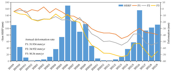
Figure 9.
The cumulative displacement curves of typical points and monthly HSRPs of the landslide.
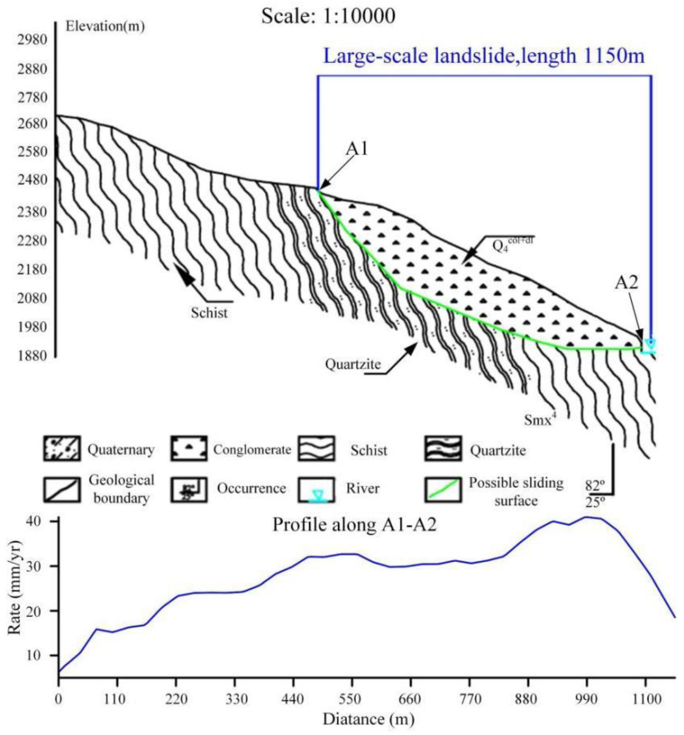
Moreover, we draw a profile map of the landslide and extract a profile line from A1 to A2 in the annual deformation map (Figure 10). As seen in Figure 9 and Figure 10, the slope tongue’s rate of and accumulated deformation are the highest, those of the slope’s middle part are the second highest, and those of the slope’s back edge are the lowest. According to our field investigation, fluvial erosion by the Dajinchuan River is another triggering factor. Especially in the flood season, the river water’s level may increase by nearly 5 m with respect to its normal status, with the peak flux exceeding 650 m3/s. The hydrodynamic pressure variations induced by the rapid river-water-level’s changes may lead to instability and movement at the front edge of the landslide [42].

Figure 10.
Profile map of the landslide and the profile line along A1–A2.
In the first alignment design version, the recommended line’s mainline (K) and alternative line (B) are tunneled through the slope’s back edge and middle part, respectively. The annual movement rate of the geometric center point on the landslide is approximately 36 mm/yr, which is higher than “30 mm/yr”, and the corresponding ASPMP (598.75 mm) is higher than ASPMPM (598.57 mm). According to our method’s rule, we chose tunnel and reinforce. And because construction along line B will intensify the deformation according to the spatiotemporal evolution, the final design version selects the mainline (K).
4.4. Landslide-Hazard-Avoiding Alignment Selection
From the above selection case, the 79 remaining landslides can be reconsidered legitimately for the first alignment design version. As described in Table 3, 33 landslides in total had a high impact (including the above case), 1 landslide had a moderate impact, and 3 landslides in total had a low impact (The other landslides far away from the line had no impact and, therefore, are not mentioned in the table.). The annual rates and ASPMPs of the landslides were extracted to obtain solutions for the alignment selection. As Table 3 shows, 13 type A, 16 type B, and 8 type C were selected for every landslide. And the corresponding final alignment design version was applied for the BKHC construction.
Table 3.
The impacts of the landslides on the study area and the corresponding advice for the alignment design.
5. Discussion
5.1. Advantages
Because of the tremendous costs caused by design alterations, a risk-optimal highway alignment selection is essential before the construction. Thus, monitoring and stability analyses of landslides are vital through the whole alignment-design workflow. Compared with traditional methods, the new systematic highway alignment selection approach we proposed combines the CSI and ~1 km monthly HSRP analysis. It can give a more accurate quantitative reference to help to finalize the alignment.
As the fundamental tool in landslide monitoring, TS–InSAR has to face spatiotemporal decorrelations, atmospheric delay anomalies, geometric distortions, etc., especially in the mountainous area in southwestern China [14,15,16,17,18,19,20]. Consequently, SqueeSARTM has been widely employed to solve a part of these problems, in some period of time, as a representative next-generation TS–InSAR technique. After reviewing the existing research about SqueeSARTM, we found that it has evolved to series of algorithms [35,36,37,38,39,40,41,42], from which we selected the CSI as the key step of our method to provide a much denser observation network for performing more reliable phase unwrapping to obtain more accurate MPs.
However, no matter which algorithm is utilized, geometric distortion still restricts the accuracy and effectiveness for monitoring from the root. In most studies or actual projects, both the ascending and descending SAR images are used without any FS analysis. The tremendous data redundancy reduces the TS–InSAR’s efficiency, especially in wide ranges. Therefore, in our method, data selection is regarded as being the first key step based on FS calculations, which can reduce the data downloading and processing times.
Rainfall is the most important factor inducing landslides, especially in the rainy season. After obtaining enough deformation signals and accurate rates of landslides, the accuracy of the precipitation data should be improved as well. In the mountainous area of southwestern China, high-spatial-resolution precipitation data cannot be obtained because of the low station density, even with the establishment of additional stations in recent years [53,54,55,56,57,58,59]. On reviewing the related research, we found that the station density decides the result accuracy of conventional interpolation methods, including inverse distance weighting, kriging methods, and regression analysis. Thus, delta spatial downscaling is used to obtain the ~1 km HSRP at the local scale based on CRU time-series datasets and WorldClim climatology datasets in our method. Compared with the data from the climate stations far from the BKHC, the HSRP exhibits smaller deviations and is more accurate [60,61,62,63,64,65,66]. Moreover, our method extracted the ASPMP of every landslide and ASPMPM based on the HSRP, which would result in a reasonable reference index for the alignment selection.
Herein, our method incorporated the advantages of these new techniques, attempted to combine all the accurate results, and considered the locations and deformation rates of landslides and ASPMPs as the major factors, while construction possibly impacts the secondary factors. On these bases, the risk-optimal highway alignment can be finalized reasonably and efficiently based on our three solution types.
5.2. Limitations and Further Directions
Regardless of the TS–InSAR method’s advantages that we incorporated, the computational expense of the CSI is still unacceptable for a normal computer. In our case study, we used a computer with an i9-11900 CPU, a 128 GB RAM, and a 4 TB hard disk to conduct the experiments. Hence, how to improve the computational efficiency and reduce the consumption of the storage space have become critical problems to be solved. Moreover, L-band images have more penetration and X-band images have a higher resolution than C-band images, respectively. We only processed C-band SAR images, but the other two types of band images were not tested. It is expected that our method can not only benefit from them but also face computing and FS-analyzing challenges. In addition, the Generic Atmospheric Correction Online Service’s (GACOS’s) atmospheric delay products were not used in our method to improve the accuracy of the monitoring, which can provide a new approach for the atmospheric correction of repeat-pass InSAR [75].
As for the HSRP analysis, the data-downscaling method was employed for the 30′ CRU and WorldClim time-series data in our method after reviewing previous studies [65,66]. However, on one hand, the averaged 30′ elevation was used for the original CRU data, which weakened the representation of the precipitation on the actual land surface, especially in the mountainous area. On the other hand, the weather stations used for the CRU evaluation are located in valleys near counties or cities, which cannot reflect the real conditions of wilderness areas. Meanwhile, as the reference climatology dataset, the WorldClim dataset performed well. But a new and better reference climatology dataset needs to be generated for southwestern China, and the collection of public and private climate data can be a good solution.
There are many other environmental factors that affect landslide stability, such as earthquakes, reservoir impoundments, fluvial erosion, and weathering. But in the final step of our method, we only selected the ASPMP as the dominant environmental factor to help to select the alignment. In practice, other factors should be considered comprehensively to establish a judgement model. For instance, landslides are typical post-disasters of earthquakes, especially in the eastern margin of the Qinghai–Tibetan Plateau. This region is a very active seismic area in which three major earthquakes have been recorded since the 1930s, namely, the 1933 Mw 7.3 Diexi earthquake, the 1976 Mw 6.7 Songpan–Pingwu earthquake, and the 2008 Mw 7.9 Wenchuan earthquake. During these strong seismic activities, the rock mass was damaged by the discordant deformation from different existing lithologies. Hence, the locations of earthquake zones should be considered synthetically for better highway alignment selections in future work. And the possible impacts of construction on landslides need a quantitative analysis rather than just a qualitative deduction.
In the future, our research emphasis will focus on parallel computing, automatic processing based on deep-learning models, more landslide-event-training samples, multi-platform SAR images, higher-spatial-resolution DEMs, etc.
6. Conclusions
In this study, a section of the BKHC was taken as the study area, which has a severe alignment design problem due to the complicated geological background, strong tectonic movement, rock body rupture, as well as frequent geohazards. Hence, this paper proposed a new systematic highway alignment selection method for a typical section of the BKHC, which has 80 slow-moving landslides identified by optical remote-sensing interpretation and field investigation, based on CSI and ~1 km monthly HSRP analysis.
Specifically, the FSs of Sentinel-1A ascending and descending images were first calculated to select suitable SAR datasets according to the locations of identified landslides. Consequently, 56 Sentinel-1A descending images from September 2019 to September 2021 were processed using CSI and SBAS-InSAR to obtain the time-series deformation and rates of landslides and illustrate the strengths of the CSI. The results reveal that CSI has clearer deformation signals and more MPs than SBAS-InSAR. And the maximum cumulative displacements and rates of the landslides reach −75 mm and −64 mm/yr within the monitoring period (CSI results), respectively. To demonstrate the applicability of our method to every landslide, we selected the largest landslide as a typical case. Through further spatiotemporal evolution analysis of this case, we found that accelerated sliding is highly related to intense rainfall events and that fluvial erosion impacts the slope’s stability perennially. Under this circumstance, we utilized delta downscaling to obtain the ~1 km HSRP based on CRU and WorldClim time-series data, and the ASPMPs of every landslide were extracted afterward. Subsequently, three solution types were established in our method by setting thresholds for deformation rates and ASPMPs. Finally, the risk-optimal alignment selection of the BKHC was reasonably and efficiently finalized based on these solution types and the construction’s possible impacts.
This proposed method expands the application range of the TS–InSAR in actual transport engineering and reduces the time and economic and labor costs associated with recurrent landslides. Though some limitations need to be resolved in the future, these research results offer a valuable consultation for the alignment selection of highways in mountainous areas and, consequently, for landslide management.
Author Contributions
Conceptualization, Z.W.; methodology, Z.W.; software, X.S.; validation, Y.J., S.L. and R.Z.; formal analysis, Z.W.; investigation, Z.W.; resources, Z.W.; data curation, B.X.; writing—original draft preparation, Z.W.; writing—review and editing, Z.W.; visualization, Z.W.; supervision, Y.J. and R.Z.; project administration, S.L.; funding acquisition, Y.J. and Z.W. All authors have read and agreed to the published version of the manuscript.
Funding
This study was funded by the Sichuan Provincial Science and Technology Department’s key research projects (2023YFS0434), the Sichuan Society of Surveying and Mapping Geo-information’s open fund (CCX202305), the Sichuan Provincial Transportation Department’s research projects (2023-A-14), and the Key Laboratory of Land Satellite Remote Sensing Application, Ministry of Natural Resources open fund (KLSMNR-202309).
Data Availability Statement
CRU TS v. 4.07 data can be downloaded from the website https://crudata.uea.ac.uk/cru/data/hrg/cru_ts_4.07/ (accessed on 1 April 2023); WorldClim v. 2.1 data can be downloaded from the website https://worldclim.org/data/monthlywth.html (accessed on 1 April 2023); the POD can be downloaded from the website https://s1qc.asf.alaska.edu/aux_poeorb/ (accessed on 1 April 2023); the Sentinel-1A SAR images can be downloaded from the website https://scihub.copernicus.eu/dhus/#/home (accessed on 1 April 2023).
Acknowledgments
The Sentinel-1A satellite images and POD data used in this paper are provided by the Copernicus Sentinel-1 Mission of the ESA. The SRTM DEM data are provided by NASA.
Conflicts of Interest
Authors Zhiheng Wang, Yang Jia, Shengfu Li, Binzhi Xu and Xiaopeng Sun were employed by the Sichuan Highway Planning, Survey, Design and Research Institute Ltd. The remaining authors declare that the research was conducted in the absence of any commercial or financial relationships that could be construed as a potential conflict of interest.
References
- Confuorto, P.; Angrisani, A.; Novellino, A.; Infante, D.; Calcaterra, D. A Combined Procedure Using Satellite-Based Differential SAR Interferometry and Field Measurements for Landslide Characterization in Small Urban Settings. In Proceedings of the FRINGE 2017, Helsinki, Finland, 5–9 June 2017. [Google Scholar]
- Nikolaeva, R.V. Road safety as a factor in the socio-economic development of the country. IOP Conf. Ser. Mater. Sci. Eng. 2020, 786, 012070. [Google Scholar] [CrossRef]
- Ismail, K.; Sayed, T. Risk-optimal highway design: Methodology and case studies. Saf. Sci. 2012, 50, 1513–1521. [Google Scholar] [CrossRef]
- Yin, C.; Zhang, J. Hazard regionalization of debris-flow disasters along highways in China. Nat. Hazards 2018, 91, 129–147. [Google Scholar] [CrossRef]
- Pandey, V.K.; Sharma, M.C. Probabilistic landslide susceptibility mapping along Tipri to Ghuttu highway corridor, Garhwal Himalaya (India). Remote Sens. Appl. Soc. Environ. 2017, 8, 1–11. [Google Scholar] [CrossRef]
- Tang, H.; Gong, W.; Li, C.; Wang, L.; Juang, C.H. A new framework for characterizing landslide deformation: A case study of the Yu-Kai highway landslide in Guizhou, China. Bull. Eng. Geol. Environ. 2018, 78, 4291–4309. [Google Scholar] [CrossRef]
- Huang, Y.; Yi, S.; Li, Z.; Shao, S.; Qin, X. Design of highway landslide warning and emergency response systems based on UAV. In Proceedings of the Seventeenth China Symposium on Remote Sensing, Hangzhou, China, 27–31 August 2010; International Society for Optics and Photonics: Bellingham, WA, USA, 2011. [Google Scholar]
- Xu, C.; Tian, Y.; Zhou, B.; Ran, H.; Lyu, G. Landslide damage along Araniko Highway and Pasang Lhamu Highway and regional assessment of landslide hazard related to the Gorkha, Nepal earthquake of 25 April 2015. Geoenviron. Disasters 2017, 4, 14. [Google Scholar] [CrossRef]
- Psomiadis, E.; Papazachariou, A.; Soulis, K.X.; Alexiou, D.S.; Charalampopoulos, I. Landslide mapping and susceptibility assessment using geospatial analysis and earth observation data. Land 2020, 9, 133. [Google Scholar] [CrossRef]
- Qiu, H.; Su, L.; Tang, B.; Yang, D.; Ullah, M.; Zhu, Y.; Kamp, U. The effect of location and geometric properties of landslides caused by rainstorms and earthquakes. Earth Surf. Process. Landf. 2024; early view. [Google Scholar] [CrossRef]
- Ye, B.; Qiu, H.; Tang, B.; Liu, Y.; Liu, Z.; Jiang, X.; Yang, D.; Ullah, M.; Zhu, Y.; Kamp, U. Creep deformation monitoring of landslides in a reservoir area. J. Hydrol. 2024, 632, 130905. [Google Scholar] [CrossRef]
- Liu, Y.; Qiu, H.; Kamp, U.; Wang, N.; Wang, J.; Huang, C.; Tang, B. Higher temperature sensitivity of retrogressive thaw slump activity in the Arctic compared to the Third Pole. Sci. Total Environ. 2024, 914, 170007. [Google Scholar] [CrossRef] [PubMed]
- Yang, D.; Qiu, H.; Ye, B.; Liu, Y.; Zhang, J.; Zhu, Y. Distribution and Recurrence of Warming-Induced Retrogressive Thaw Slumps on the Central Qinghai-Tibet Plateau. J. Geophys. Res. Earth Surf. 2023, 128, e2022JF007047. [Google Scholar] [CrossRef]
- Berardino, P.; Fornaro, G.; Lanari, R.; Sansosti, E. A new algorithm for surface deformation monitoring based on small baseline differential SAR interferograms. IEEE Trans. Geosci. Remote Sens. 2002, 40, 2375–2383. [Google Scholar] [CrossRef]
- Ferretti, A.; Prati, C.; Rocca, F. Permanent scatterers in SAR interferometry. IEEE Trans. Geosci. Remote Sens. 2001, 39, 8–20. [Google Scholar] [CrossRef]
- Hooper, A. A multi-temporal InSAR method incorporating both persistent scatterer and small baseline approaches. Geophys. Res. Lett. 2008, 35, 96–106. [Google Scholar] [CrossRef]
- Hooper, A.; Zebker, H.; Segall, P.; Kampes, B. A new method for measuring deformation on volcanoes and other natural terrains using InSAR persistent scatterers. Geophys. Res. Lett. 2004, 31, L23611. [Google Scholar] [CrossRef]
- Iglesias, R.; Mallorqui, J.; Monells, D.; López-Martínez, C.; Fabregas, X.; Aguasca, A.; Gili, J.; Corominas, J. PSI deformation map retrieval by means of temporal sublook coherence on reduced sets of SAR images. Remote Sens. 2015, 7, 530. [Google Scholar] [CrossRef]
- Lanari, R.; Mora, O.; Manunta, M.; Mallorquí, J.J.; Berardino, P.; Sansosti, E. A small-baseline approach for investigating deformations on full-resolution differential SAR interferograms. IEEE Trans. Geosci. Remote Sens. 2004, 42, 1377–1386. [Google Scholar] [CrossRef]
- Mora, O.; Mallorqui, J.J.; Broquetas, A. Linear and nonlinear terrain deformation maps from a reduced set of interferometric SAR images. IEEE Trans. Geosci. Remote Sens. 2003, 41, 2243–2253. [Google Scholar] [CrossRef]
- Werner, C.; Wegmuller, U.; Strozzi, T.; Wiesmann, A. Interferometric point target analysis for deformation mapping. In Proceedings of the IEEE International Geoscience and Remote Sensing Symposium 2003, Toulouse, France, 21–25 July 2003; pp. 4362–4364. [Google Scholar]
- Bovenga, F.; Refice, A.; Nutricato, R.; Guerriero, L.; Chiaradia, M. SPINUA: A flexible processing chain for ERS/ENVISAT long term interferometry. In Proceedings of the ESA-ENVISAT Symposium, Salzburg, Austria, 6–10 September 2004; pp. 6–10. [Google Scholar]
- Bovenga, F.; Nutricato, R.; Refice, A.; Wasowski, J. Application of multi-temporal differential interferometry to slope instability detection in urban/peri-urban areas. Eng. Geol. 2006, 88, 218–239. [Google Scholar] [CrossRef]
- Kampes, B. Radar Interferometry: Persistent Scatterer Technique; Springer: Berlin/Heidelberg, Germany, 2006. [Google Scholar]
- Crosetto, M.; Biescas, E.; Duro, J.; Closa, J.; Arnaud, A. Generation of advanced ERS and Envisat interferometric SAR products using the stable point network technique. Photogramm. Eng. Remote Sens. 2008, 74, 443–450. [Google Scholar] [CrossRef]
- Kuehn, F.; Albiol, D.; Cooksley, G.; Duro, J.; Granda, J.; Haas, S.; Hoffmann-Rothe, A.; Murdohardono, D. Detection of land subsidence in Semarang, Indonesia, using stable points network (SPN) technique. Environ. Earth Sci. 2010, 60, 909–921. [Google Scholar] [CrossRef]
- Costantini, M.; Falco, S.; Malvarosa, F.; Minati, F. A new method for identification and analysis of persistent scatterers in series of SAR images. In Proceedings of the IEEE International Geoscience and Remote Sensing Symposium 2008, Boston, MA, USA, 8–11 July 2008; pp. 449–452. [Google Scholar]
- Costantini, M.; Falco, S.; Malvarosa, F.; Minati, F.; Trillo, F.; Vecchioli, F. Persistent scatterer pair interferometry: Approach and application to COSMO-SkyMed SAR data. IEEE J. Sel. Top. Appl. Earth Obs. Remote Sens. 2014, 7, 2869–2879. [Google Scholar] [CrossRef]
- Casu, F.; Manzo, M.; Lanari, R. A quantitative assessment of the SBAS algorithm performance for surface deformation retrieval from DInSAR data. Remote Sens. Environ. 2006, 102, 195–210. [Google Scholar] [CrossRef]
- Schmidt, D.; Bürgmann, R. Time-dependent land uplift and subsidence in the Santa Clara valley, California, from a large interferometric synthetic aperture radar dataset. J. Geophys. Res. Solid. Earth 2003, 108, 2416. [Google Scholar] [CrossRef]
- Perissin, D.; Wang, T. Repeat-pass SAR interferometry with partially coherent targets. IEEE Trans. Geosci. Remote Sens. 2012, 50, 271–280. [Google Scholar] [CrossRef]
- Zhang, L.; Ding, X.; Lu, Z. Ground settlement monitoring based on temporarily coherent points between two SAR acquisitions. ISPRS J. Photogramm. Remote Sens. 2011, 66, 146–152. [Google Scholar] [CrossRef]
- Zhang, L.; Lu, Z.; Ding, X.; Jung, H.-S.; Feng, G.; Lee, C. Mapping ground surface deformation using temporarily coherent point SAR interferometry: Application to Los Angeles Basin. Remote Sens. Environ. 2012, 117, 429–439. [Google Scholar] [CrossRef]
- Ferretti, A.; Fumagalli, A.; Novali, F.; Prati, C.; Rocca, F.; Rucci, A. A new algorithm for processing interferometric data-stacks: SqueeSAR. IEEE Trans. Geosci. Remote Sens. 2011, 49, 3460–3470. [Google Scholar] [CrossRef]
- Zhu, J.; Hu, J.; Li, Z.; Sun, Q.; Zheng, W. Recent progress in landslide monitoring with InSAR. Acta Geod. Cartogr. Sin. 2022, 51, 2001–2019. [Google Scholar]
- Lv, X.; Yazıcı, B.; Zeghal, M.; Bennett, V. Joint-scatterer processing for time-series InSAR. IEEE Trans. Geosci. Remote Sens. 2014, 52, 7205–7722. [Google Scholar]
- Fornaro, G.; Verde, S.; Reale, D.; Pauciullo, A. CAESAR: An approach based on covariance matrix decomposition to improve multibaseline–multitemporal interferometric SAR processing. IEEE Trans. Geosci. Remote Sens. 2015, 53, 2050–2065. [Google Scholar] [CrossRef]
- Cao, N.; Lee, H.; Jung, H.C. A phase-decomposition-based PSInSAR processing method. IEEE Trans. Geosci. Remote Sens. 2015, 54, 1074–1090. [Google Scholar] [CrossRef]
- Du, Z.; Ge, L.; Li, X.; Ng, A. Subsidence monitoring over the southern coalfield, Australia using both L-band and C-band SAR time series analysis. Remote Sens. 2016, 8, 543. [Google Scholar] [CrossRef]
- Ge, L.; Ng, A.H.-M.; Li, X.; Abidin, H.Z.; Gumilar, I. Land subsidence characteristics of Bandung Basin as revealed by ENVISAT ASAR and ALOS PALSAR interferometry. Remote Sens. Environ. 2014, 154, 46–60. [Google Scholar] [CrossRef]
- Ng, A.; Ge, L.; Li, X. Assessments of land subsidence in the Gippsland Basin of Australia using ALOS PALSAR data. Remote Sens. Environ. 2015, 159, 86–101. [Google Scholar] [CrossRef]
- Dong, J.; Zhang, L.; Tang, M.; Liao, M.; Xu, Q.; Gong, J.; Ao, M. Mapping landslide surface displacements with time series sar interferometry by combining persistent and distributed scatterers: A case study of jiaju landslide in danba, china. Remote Sens. Environ. 2018, 205, 180–198. [Google Scholar] [CrossRef]
- Solari, L.; Del Soldato, M.; Raspini, F.; Barra, A.; Bianchini, S.; Confuorto, P.; Casagli, N.; Crosetto, M. Review of satellite interferometry for landslide detection in Italy. Remote Sens. 2020, 12, 1351. [Google Scholar] [CrossRef]
- Tsironi, V.; Ganas, A.; Karamitros, I.; Efstathiou, E.; Koukouvelas, I.; Sokos, E. Kinematics of active landslides in Achaia (Peloponnese, Greece) through InSAR time series analysis and relation to rainfall patterns. Remote Sens. 2022, 14, 844. [Google Scholar] [CrossRef]
- Dai, K.; Chen, Y.; Xu, Q.; Hancock, C.; Jiang, M.; Deng, J.; Zhuo, G. A functional model for determining maximum detectable deformation gradients of InSAR considering the topography in mountainous areas. IEEE Trans. Geosci. Remote Sens. 2023, 61, 5211211. [Google Scholar] [CrossRef]
- Deng, Y.; Zuo, X.; Li, Y.; Zhou, X. Landslide susceptibility evaluation of Bayesian optimized CNN Gengma seismic zone considering InSAR deformation. Appl. Sci. 2023, 13, 11388. [Google Scholar] [CrossRef]
- Cohen-Waeber, J.; Bürgmann, R.; Chaussard, E.; Giannico, C.; Ferretti, A. Spatiotemporal patterns of precipitation-modulated landslide deformation from independent component analysis of InSAR time series. Geophys. Res. Lett. 2018, 45, 1878–1887. [Google Scholar] [CrossRef]
- Intrieri, E.; Raspini, F.; Fumagalli, A.; Lu, P.; Del Conte, S.; Farina, P.; Allievi, J.; Ferretti, A.; Casagli, N. The Maoxian landslide as seen from space: Detecting precursors of failure with Sentinel-1 data. Landslides 2018, 15, 123–133. [Google Scholar] [CrossRef]
- Bellotti, F.; Bianchi, M.; Colombo, D.; Ferretti, A.; Tamburini, A. Advanced InSAR Techniques to Support Landslide Monitoring; Springer: Berlin/Heidelberg, Germany, 2014. [Google Scholar]
- Zhang, L.; Dai, K.; Deng, J.; Ge, D.; Liang, R.; Li, W.; Xu, Q. Identifying Potential Landslides by Stacking-InSAR in Southwestern China and Its Performance Comparison with SBAS-InSAR. Remote Sens. 2021, 13, 3662. [Google Scholar] [CrossRef]
- Zhou, H.; Dai, K.; Pirasteh, S.; Li, R.; Xiang, J.; Li, Z. InSAR spatial-heterogeneity tropospheric delay correction in steep mountainous areas based on deep learning for landslides monitoring. IEEE Trans. Geosci. Remote Sens. 2023, 61, 5215014. [Google Scholar] [CrossRef]
- Dai, K.; Li, Z.; Xu, Q.; Bürgmann, R.; Milledge, D.; Tomás, R.; Fan, X.; Zhao, C.; Liu, X.; Peng, J.; et al. Entering the Era of Earth Observation-Based Landslide Warning Systems: A Novel and Exciting Framework. IEEE Geosci. Remote Sens. Mag. 2020, 8, 136–153. [Google Scholar] [CrossRef]
- Peng, S.; Gang, C.; Cao, Y.; Chen, Y. Assessment of climate change trends over the Loess Plateau in China from 1901 to 2100. Int. J. Climatol. 2018, 38, 2250–2264. [Google Scholar] [CrossRef]
- Li, Z.; Zheng, F.; Liu, W.; Flanagan, D.C. Spatial distribution and temporal trends of extreme temperature and precipitation events on the Loess Plateau of China during 1961–2007. Quat. Int. 2010, 226, 92–100. [Google Scholar] [CrossRef]
- Li, Z.; Zheng, F.L.; Liu, W.Z. Spatiotemporal characteristics of reference evapotranspiration during 1961–2009 and its projected changes during 2011–2099 on the Loess Plateau of China. Agric. For. Meteorol. 2012, 154, 147–155. [Google Scholar] [CrossRef]
- Zhao, C.; Nan, Z.; Feng, Z. GIS-assisted spatially distributed modeling of the potential evapotranspiration in semi-arid climate of the Chinese Loess Plateau. J. Arid. Environ. 2003, 58, 387–403. [Google Scholar]
- Rahman, A.-u.; Dawood, M. Spatio-statistical analysis of temperature fluctuation using Mann–Kendall and Sen’s slope approach. Clim. Dyn. 2017, 48, 783–797. [Google Scholar] [CrossRef]
- Peng, S.; Zhao, C.; Wang, X.; Xu, Z.; Liu, X.; Hao, H.; Yang, S. Mapping daily temperature and precipitation in the Qilian Mountains of northwest China. J. Mt. Sci. 2016, 11, 896–905. [Google Scholar] [CrossRef]
- Gao, L.; Wei, J.; Wang, L.; Bernhardt, M.; Schulz, K.; Chen, X. A high-resolution air temperature data set for the Chinese Tian Shan in 1979–2016. Earth Syst. Sci. Data 2018, 10, 2097–2114. [Google Scholar] [CrossRef]
- Brekke, L.; Thrasher, B.; Maurer, E.; Pruitt, T. Downscaled CMIP3 and CMIP5 Climate and Hydrology Projections: Release of Downscaled CMIP5 Climate Projections, Comparison with Preceding Information, and Summary of User Needs; U.S. Department of the Interior, Bureau of Reclamation, Technical Services Center: Denver, CO, USA, 2013.
- Harris, I.; Jones, P.; Osborn, T.; Lister, D. Updated high–resolution grids of monthly climatic observations the CRU TS3.10 Dataset. Int. J. Climatol. 2014, 34, 623–642. [Google Scholar] [CrossRef]
- Becker, A.; Finger, P.; Meyer-Christoffer, A.; Rudolf, B.; Schamm, K.; Schneider, U.; Ziese, M. A description of the global land-surface precipitation data products of the Global Precipitation Climatology Centre with sample applications including centennial (trend) analysis from 1901–present. Earth Syst. Sci. Data 2013, 5, 71–99. [Google Scholar] [CrossRef]
- Mosier, T.M.; Hill, D.F.; Sharp, K.V. 30-Arcsecond monthly climate surfaces with global land coverage. Int. J. Climatol. 2014, 34, 2175–2188. [Google Scholar] [CrossRef]
- Wang, L.; Chen, W. A CMIP5 multimodel projection of future temperature, precipitation, and climatological drought in China. Int. J. Climatol. 2014, 34, 2059–2078. [Google Scholar] [CrossRef]
- Peng, S.; Ding, Y.; Liu, W.; Li, Z. 1 km monthly temperature and precipitation dataset for China from 1901 to 2017. Earth Syst. Sci. Data 2019, 11, 1931–1946. [Google Scholar] [CrossRef]
- Harris, I.; Osborn, T.J.; Jones, P.; Lister, D. Version 4 of the CRU TS monthly high-resolution gridded multivariate climate dataset. Sci. Data 2020, 7, 109. [Google Scholar] [CrossRef] [PubMed]
- Dai, K.; Li, Z.; Tomás, R.; Liu, G.; Yu, B.; Wang, X.; Cheng, H.; Chen, J.; Stockamp, J. Monitoring activity at the Daguangbao mega-landslide (China) using Sentinel-1 TOPS time series interferometry. Remote Sens. Environ. 2016, 186, 501–513. [Google Scholar] [CrossRef]
- Del Soldato, M.; Solari, L.; Novellino, A.; Monserrat, O.; Raspini, F. A new set of tools for the generation of InSAR visibility maps over wide areas. Geosciences 2021, 11, 229. [Google Scholar] [CrossRef]
- Hooper, A.; Segall, P.; Zebker, H. Persistent scatterer InSAR for crustal deformation analysis, with application to Volcán Alcedo, Galápagos. J. Geophys. Res. Solid Earth 2007, 112, B07407. [Google Scholar] [CrossRef]
- Jiang, M.; Ding, X.; Hanssen, R.F.; Malhotra, R.; Chang, L. Fast statistically homogeneous pixel selection for covariance matrix estimation for multitemporal InSAR. IEEE Trans. Geosci. Remote Sens. 2015, 53, 1213–1224. [Google Scholar] [CrossRef]
- Monti Guarnieri, A.; Tebaldini, S. On the exploitation of target statistics for SAR interferometry applications. IEEE Trans. Geosci. Remote Sens. 2008, 46, 3436–3443. [Google Scholar] [CrossRef]
- Hooper, A.; Bekaert, D.; Spaans, K.; Arıkan, M. Recent advances in SAR interferometry time series analysis for measuring crustal deformation. Tectonophysics 2012, 514–517, 1–13. [Google Scholar] [CrossRef]
- Liu, X.; Zhao, C.; Zhang, Q.; Lu, Z.; Li, Z.; Yang, C.; Zhu, W.; Liu-Zeng, J.; Chen, L.; Liu, C. Integration of Sentinel-1 and ALOS/PALSAR-2 SAR datasets for mapping active landslides along the Jinsha River corridor, China. Eng. Geol. 2021, 284, 106033. [Google Scholar] [CrossRef]
- Duan, X.; Hou, T.S.; Jiang, X.D. Study on stability of exit slope of Chenjiapo tunnel under extreme rainstorm conditions. Nat. Hazards 2021, 107, 1387–1411. [Google Scholar] [CrossRef]
- Wang, Q.; Yu, W.; Xu, B.; Wei, G. Assessing the Use of GACOS Products for SBAS-InSAR Deformation Monitoring: A Case in Southern California. Sensors 2019, 19, 3894. [Google Scholar] [CrossRef] [PubMed]


Disclaimer/Publisher’s Note: The statements, opinions and data contained in all publications are solely those of the individual author(s) and contributor(s) and not of MDPI and/or the editor(s). MDPI and/or the editor(s) disclaim responsibility for any injury to people or property resulting from any ideas, methods, instructions or products referred to in the content. |
© 2024 by the authors. Licensee MDPI, Basel, Switzerland. This article is an open access article distributed under the terms and conditions of the Creative Commons Attribution (CC BY) license (https://creativecommons.org/licenses/by/4.0/).