Weighted Differential Gradient Method for Filling Pits in Light Detection and Ranging (LiDAR) Canopy Height Model

Abstract

The canopy height model (CHM) derived from LiDAR point cloud data is usually used to accurately identify the position and the canopy dimension of single tree. However, local invalid values (also called data pits) are often encountered during the generation of CHM, which results in low-quality CHM and failure in the detection of treetops. For this reason, this paper proposes an innovative method, called “pixels weighted differential gradient”, to filter these data pits accurately and improve the quality of CHM. First, two characteristic parameters, gradient index (GI) and Z-score value (ZV) are extracted from the weighted differential gradient between the pit pixels and their eight neighbors, and then GIs and ZVs are commonly used as criterion for initial identification of data pits. Secondly, CHMs of different resolutions are merged, using the image processing algorithm developed in this paper to distinguish either canopy gaps or data pits. Finally, potential pits were filtered and filled with a reasonable value. The experimental validation and comparative analysis were carried out in a coniferous forest located in Triangle Lake, United States. The experimental results showed that our method could accurately identify potential data pits and retain the canopy structure information in CHM. The root-mean-squared error (RMSE) and mean bias error (MBE) from our method are reduced by between 73% and 26% and 76% and 28%, respectively, when compared with six other methods, including the mean filter, Gaussian filter, median filter, pit-free, spike-free and graph-based progressive morphological filtering (GPMF). The average F1 score from our method could be improved by approximately 4% to 25% when applied in single-tree extraction.

1. Introduction

Airborne LiDAR point cloud data is widely utilized for measuring the geometric characteristics of tree canopies [1,2,3,4,5], significantly enhancing the accuracy of estimating forest canopy cover [6,7,8], forest biomass [9], and carbon sinks [10]. In particular, the canopy height model (CHM), which is derived from LiDAR point clouds, is valuable for accurately estimating the true physical height of trees within forested areas [11,12]. This capability greatly contributes to the efficient extraction of individual tree parameters [13,14,15].

However, data pits, which are usually hidden in CHM, are a common problem that significantly impacts the quality of CHM [16]. These pits typically manifest as randomly distributed anomalies in pixels with very low height values within the canopy, making them readily visible in CHM images [17]. Several factors contribute to the occurrence of these pits. For example, during the acquisition of LiDAR point cloud data, LiDAR pulses penetrate the canopy to hit branches below the canopy and low shrubs; signals returned from the ground and the interpolation of these laser points to generate the CHM unavoidably produce data pits [18,19,20]. Laser points with large elevation errors around overlapping airstrips also lead to data pits [21]. In addition, when the LiDAR point cloud is converted to raster data via interpolation, some points with similar x and y coordinates but with multiple elevation values can form data pits [22]. On the other hand, the density of the point cloud is another factor as well [23,24]. Pitted pixels compromise CHM accuracy, disrupt canopy surface integrity, hinder visual canopy recognition, and impact the precision of single-tree canopy extraction and crown width estimation, leading to errors in treetop extraction [25]. It has been widely accepted that one of the reasons for the underestimation of tree height is due to such pits [26]; improvement of the quality of CHMs is of great significance for subsequent research applications [27].

Researchers have proposed various methods to remove data pits in the LiDAR canopy height model. The major methods can be broadly categorized into two types: one is raster data postprocessing [28] and the other is point cloud preprocessing [29,30,31]. In the point cloud-based approach, pit-free CHMs are generated by directly processing the point cloud. Gaveau et al. [26] used only the first echoes from the LiDAR point cloud to construct the CHM. They considered that the first echo signals better represent the canopy surface information but do not detect the signals from the ground after these points and can penetrate the canopy, which becomes a potential source of error. Chen et al. [30] used the statistical Z-score [32] to remove pits for the first time. Khosravipour et al. [29] utilized all echo signals to generate a spike-free DSM that significantly reduced the data pits issue compared to using only the first echo. Hao et al. [31] proposed a graph-based progressive morphological filtering to filter out most of the non-crown points so that they could use the remaining canopy points to generate a CHM; this method reduces the data pits issue while retaining most of the canopy details. Zhang et al. developed a cloth simulation-based algorithm [33] to construct pit-free CHM from airborne LiDAR data. Parameters are usually involved in these methods, reducing the generalizability of the methods to cope with different datasets. Moreover, the point cloud preprocessing does not focus on correcting the values of error points. Instead, the number of point clouds is changed to avoid data pits during the CHM generation process. Consequently, researchers would like to recommend raster data postprocessing method for filtering data pits on CHM. Raster data are processed by constructing the CHM and then filling the pits using various image processing methods. The simplest global filters are applied to reduce the data pits issue, such as mean filtering and Gaussian filtering. These methods are simple and fast but alter the normal pixels in the CHM grayscale image and tend to result in an underestimation of canopy height [34]. Thus, it is preferable to detect pits before filling them. Ben-Arie et al. [28] filtered pits by setting a threshold and then using the median value within the window to fill the pits, but a single threshold makes it difficult to exclude the range of canopy gaps, resulting in altered values for non-pit pixels. Zhao et al. [20] improved Ben-Arie’s method by proposing the concept of canopy control to limit the canopy range, which improved the efficiency of detecting canopy pits. However, it is difficult to detect crowns with large differences in crown size under a fixed window [35]. Liu et al. [35] improved the CHM by using multiscale operators to overcome the window problem; the disadvantage of this is that multiple parameters need to be determined artificially in each multiscale operator, which makes the method rely more on manual experience and trial and error.

As outlined above, most of the studies attempted to detect data pits using single threshold or window filter but ignored the similarity between data pits and canopy gap. Therefore, this paper develops a novel method to improve the identification accuracy of data pits, which utilizes pits parameters and canopy range constraints to establish pit filtering criterion. This paper is organized as follows: Section 2 describes the methods proposed in this paper; the experiments and analysis are presented in Section 3; and the conclusions are given in Section 4.

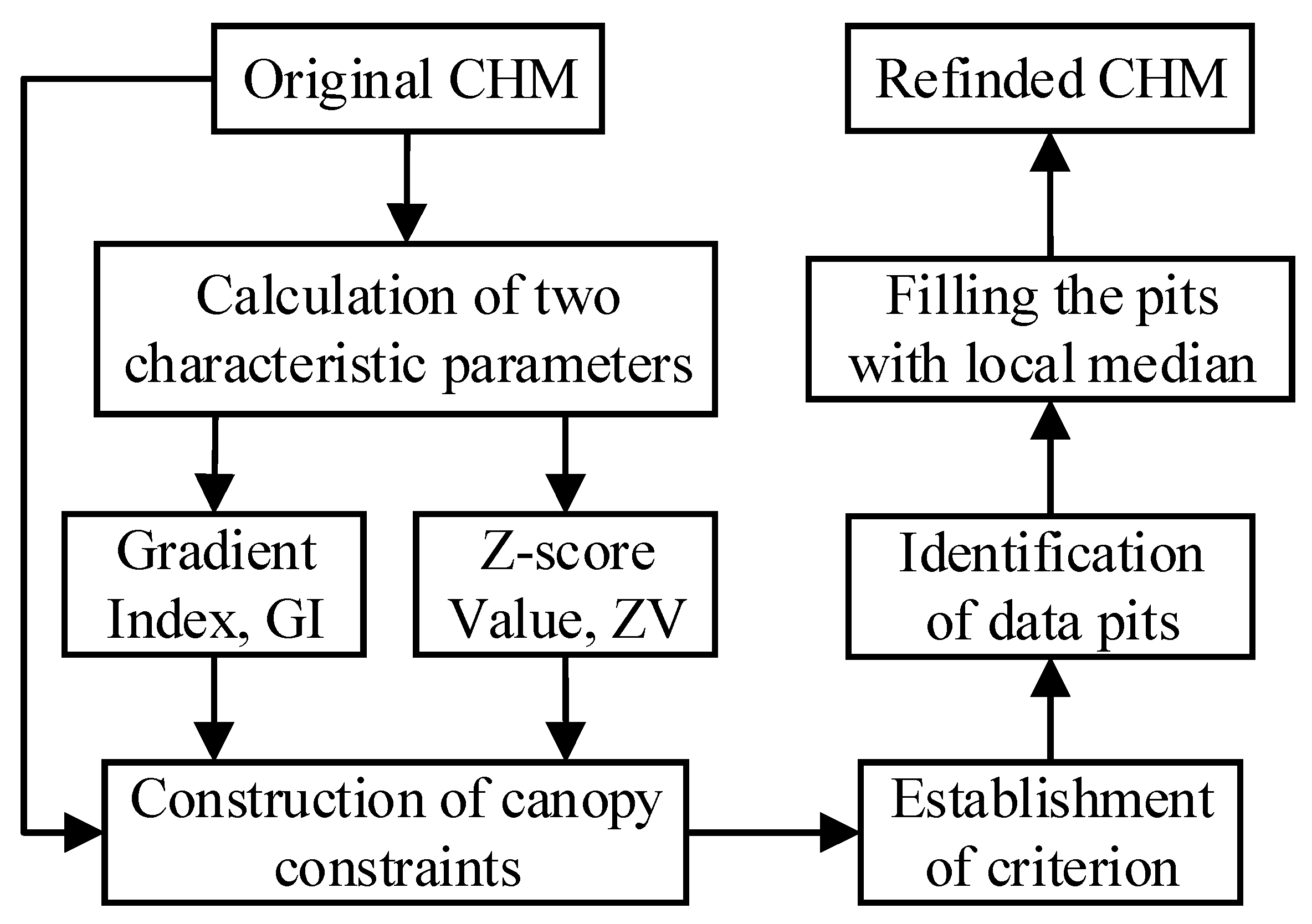
2. Development of a Weighted Differential Gradient Method

In this study, a new method is proposed for the identification of data pits to improve the accuracy of CHM. A flowchart illustrating the method proposed in this paper is shown in Figure 1; it consists of original CHM input, calculation of characteristic parameters, establishment of criterion for data pits, identification of data pits and filling them, and the refined CHM.

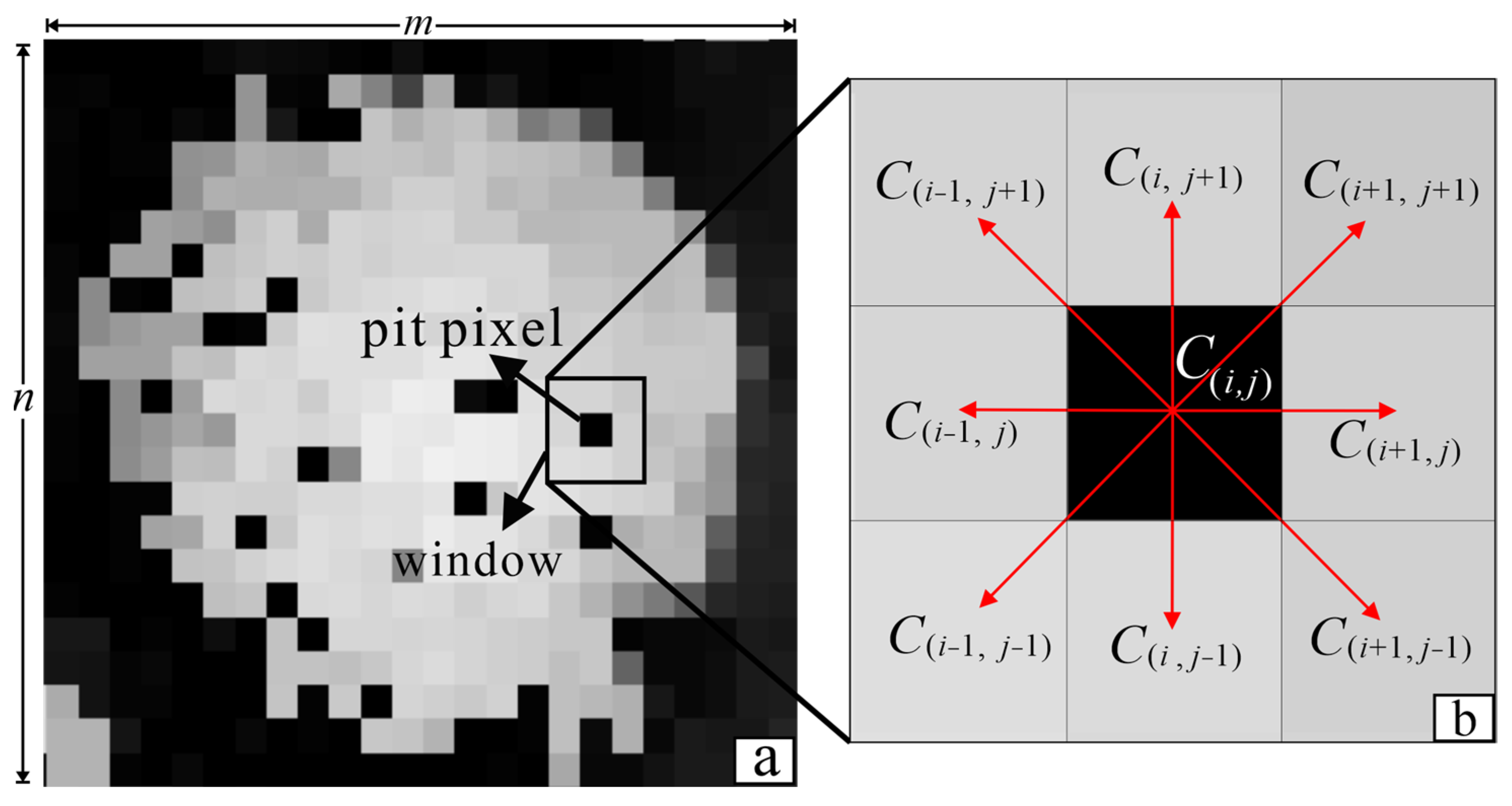
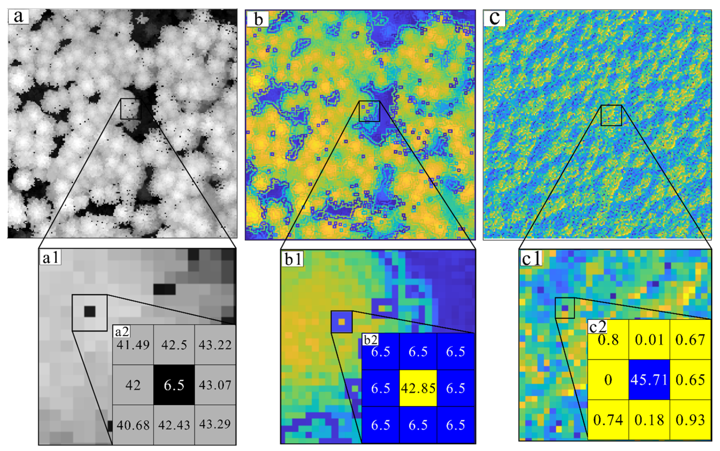
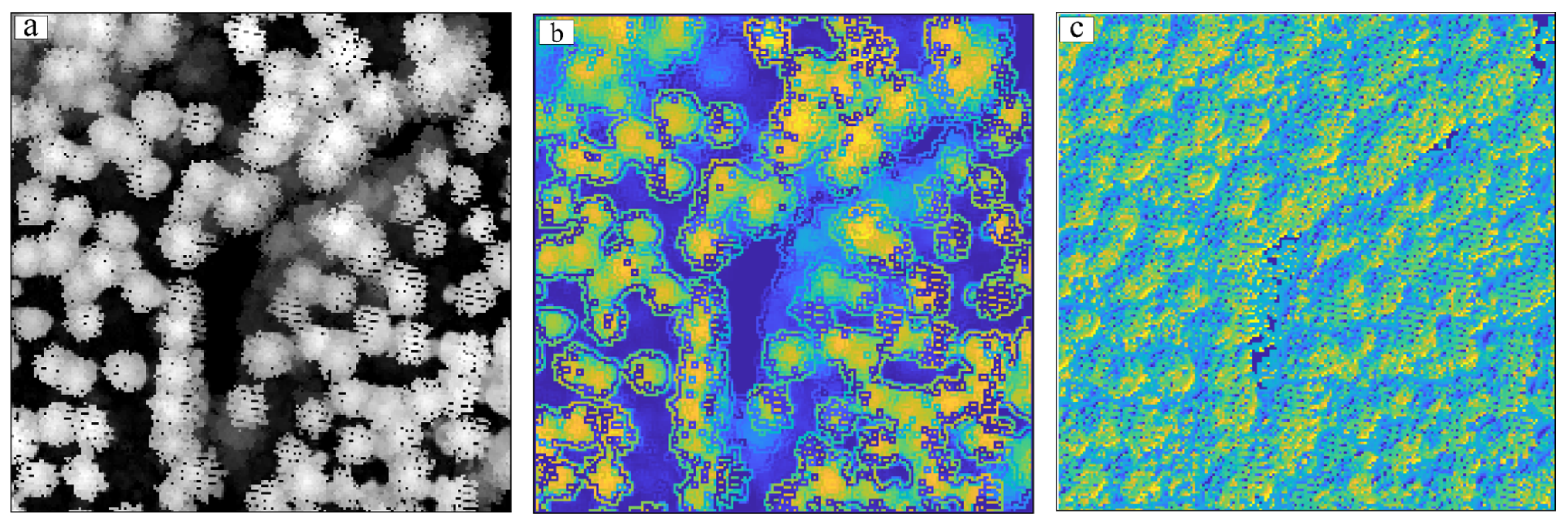
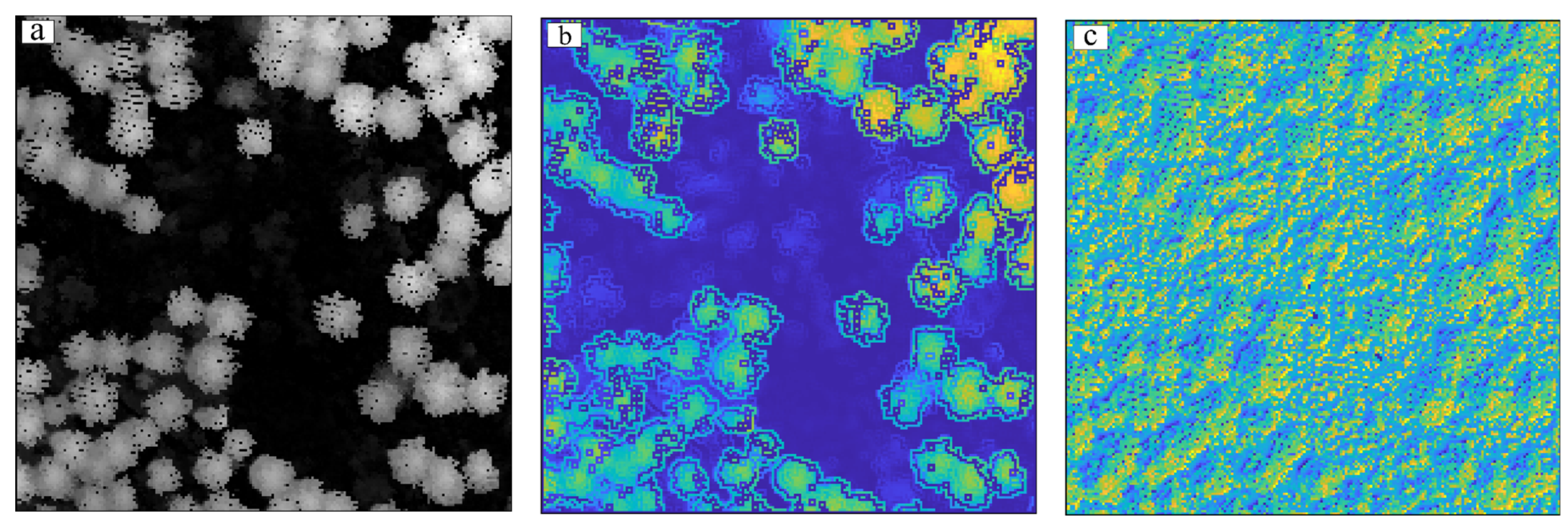
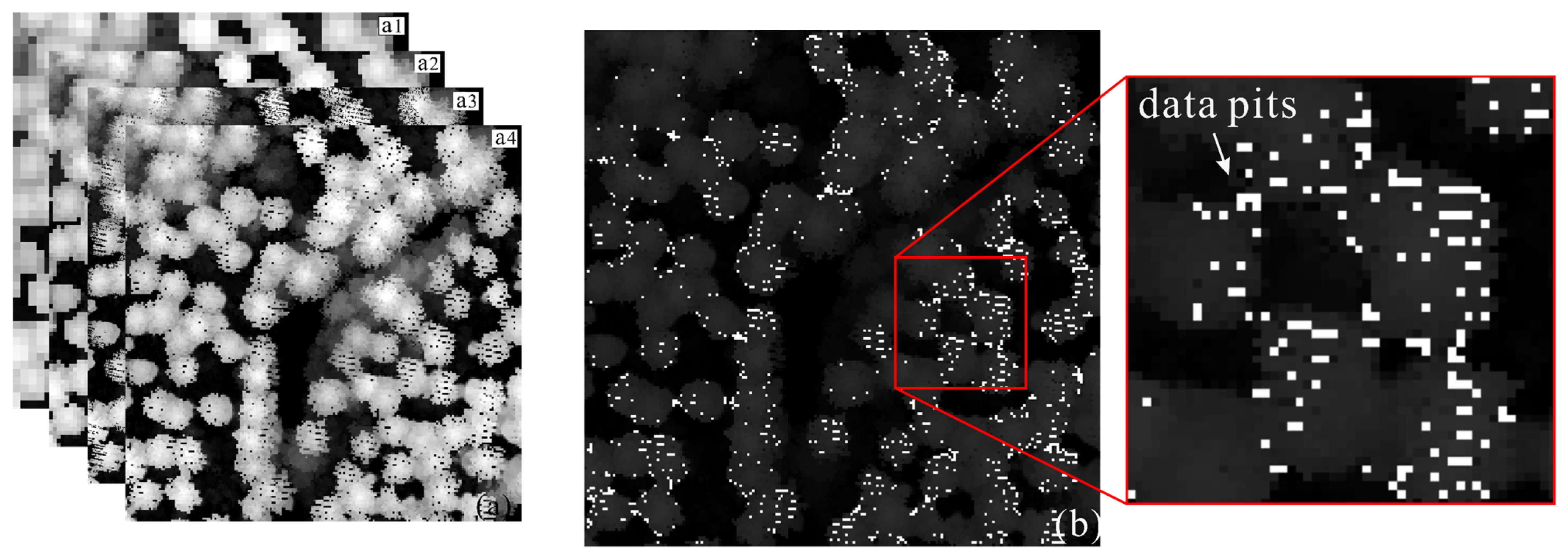
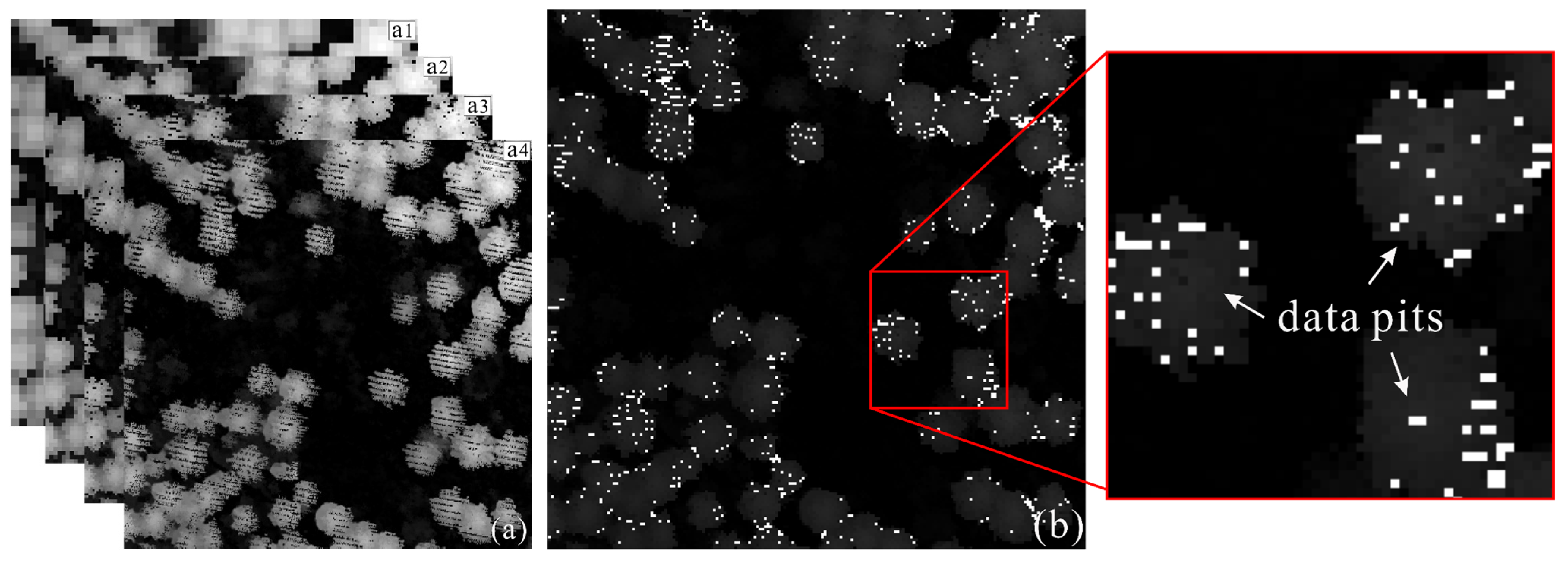
2.1. Characteristic Parameters for Canopy Pits Identification

Assuming that Figure 2a is the canopy of a tree, where the pixel with gray 0 is considered as potential pit to be identified. Further, assuming that the canopy dimension is m×n, which represents the rows and columns of the canopy image, respectively (m = 24, n = 22 in Figure 2a). In order to describe our method, a pit with a size of one pixel (i.e., called “pit pixel”) is selected (see Figure 2a), and a 3 × 3 window centralized at the pit pixel $C_{i,j}$ is selected (see Figure 2b). The nine pixels within the window are represented by {$C_{(i-1,j+1)}$, $C_{(i,j+1)}$, $C_{(i+1,j+1)}$, $C_{(i-1,j)}$, $C_{(i,j)}$, $C_{(i+1,j)}$, $C_{(i-1,j-1)}$, $C_{(i,j-1)}$, $C_{(i+1,j-1)}$}. With the nine pixels, two characteristic parameters, the Z-score, $Z{V}_{(i,j)}$, and gradient index, $G{I}_{i,j}$, can be calculated as follows:

$$Z{V}_{(i,j)}=\frac{C_{(i,j)}-M_{(i,j)}^1}{M_{(i,j)}^2},i=1,\dots ,m;j=1,\dots ,n$$

(1)

$$G{I}_{(i,j)}=\frac{{\displaystyle \sum _{i=1}^m{\displaystyle \sum _{j=1}^n\left(w_{(i,j)}\times C_{(i,j)}\right)}}}{W},i=1,\dots ,m;j=1,\dots ,n$$

(2)

where $M_{(i,j)}^1$ and $M_{(i,j)}^2$ represent the median and median absolute deviation of pixel grays within the window, respectively. $w_{(i,j)}$ and W represent the gradient weights of the eight pixel grays in the window and their sums, respectively. The parameters can be calculated as follows [25]:

$$M_{(i,j)}^1=median(C_x),x=1,\dots ,9$$

(3)

$$M_{(i,j)}^2=M_{(i,j)}^1(C_{(i,j)}-M_{(i,j)}^1),i=1,\dots ,m;j=1,\dots ,n$$

(4)

$$w_{(i,j)}=\exp (d_x),i=1,\dots ,m;j=1,\dots ,n;x=1,\dots ,8$$

(5)

$$W={\displaystyle \sum _{i=1}^m{\displaystyle \sum _{j=1}^n{w}_{(i,j)}}},i=1,\dots ,m;j=1,\dots ,n$$

(6)

where $d_x$ represents the pixel gradient within the window, which is calculated as follows:

$$\left\{\begin{array}{l}{d}_1=\left|C_{(i-1,j+1)}-C_{(i,j)}\right|,d_2=\left|C_{(i,j+1)}-C_{(i,j)}\right|\\ d_3=\left|C_{(i+1,j+1)}-C_{(i,j)}\right|,d_4=\left|C_{(i-1,j)}-C_{(i,j)}\right|\\ d_5=\left|C_{(i+1,j)}-C_{(i,j)}\right|,d_6=\left|C_{(i-1,j-1)}-C_{(i,j)}\right|\\ d_7=\left|C_{(i,j-1)}-C_{(i,j)}\right|,d_8=\left|C_{(i+1,j-1)}-C_{(i,j)}\right|\end{array}\right.,i=2,\dots ,m-2;j=2,\dots ,n-2$$

(7)

The pixel gradient in Equation (7) is indeed calculated using the gray differential between the pit pixel and their eight neighborhood pixels. Usually, the Z-score is used for detecting outliers [32], and the pit pixels of CHM are exactly considered as the outlier in gray.

2.2. Establishment of Canopy Constraints for the Weighted Differential Gradient

The method above assumed the gray with 0 as a pit pixel. In fact, the gray with 0 in a CHM does not really represent the pit pixel (see Figure 3), since the canopy gap pixels also present on a CHM with a similar gray to pit pixels. In order to disguise them, a canopy constraint $C_{(i,j)}^f(i=1,\dots ,m;j=1,\dots ,n)$ is proposed. This constraint is based so that a pit appearing on a CHM shows an abrupt height change, i.e., its height suddenly becomes lower than the ones surrounding pixels within CHM, even is sometime close to zero. Combining the gradient differential information of the pit pixels and the canopy constraints, the criteria for potential pit pixels are expressed as follows:

$$C_{(i,j)}^{pits}=\left\{\begin{array}{l}Z{V}_{(i,j)}<G{I}_{(i,j)}\\ C_{(i,j)}^f>T_C\end{array}\right.,i=1,\dots ,m;j=1,\dots ,n$$

(8)

where $C_{(i,j)}^{pits}$ is the pit in the canopy range and $T_C$ is a given threshold that should theoretically be the minimum under branch height within the measurement area. If the height value in the CHM is greater than $T_C$, it is considered to be a canopy region, and vice versa. This threshold has an impact on the accuracy of detection of canopy extent, with larger ones potentially failing to detect potential canopy areas, while smaller ones will detect information below the canopy. $C_{(i,j)}^f$ is the canopy coverage constraint, which is calculated as follows:

$$\begin{array}{c}{C}_{(i,j)}^f=k_1{C}_{c0.25(i,j)}^r+k_2{C}_{c0.5(i,j)}+k_3{C}_{c1(i,j)}^r+k_4{C}_{c2(i,j)}^r\\ (i=1,\dots ,m;j=1,\dots ,n)\end{array}$$

(9)

where $C_{c0.25(i,j)}^r,C_{c0.5(i,j)},C_{c1(i,j)}^r,C_{c2(i,j)}^r$ are CHM raster images of four different spatial resolutions, which are selected with 2.0 m, 1.0 m, 0.5 m, and 0.25 m in this paper for constructing canopy coverage constraints. Theoretically, if a canopy is visible in the raster, its spatial resolution should be lower than half of the canopy dimension [36]. On one hand, the four resolutions of CHMs are chosen to ensure that the canopy is visible in the raster and the resolution is multiplicative. On the other hand, it is difficult to deal with crowns of different sizes and canopy gaps in a single-resolution CHM image in a fixed-window convolutional operation. K represents the fusion weights, which are set on the basis of experience and to not exceed one in total. If many large canopies exist, the weights of the CHMs with resolutions of 1.0 m and 2.0 m can be set to a heavy value to reduce the information loss on the edges of large canopies. If many small canopies exist, the weights of the CHM with 0.25 m resolution can be set to heavier values to ensure the accuracy of the canopy range constraints.

Before calculating the canopy constraints, the CHMs involved in constructing the constraints must perform a morphological closure operation to recover the crown [20]. Therefore, a morphological closure operator is applied to the original CHM to recover the canopy shape (see Figure 4). Assuming that the raw CHM image is S, a morphological closure operation is performed with an approximate circular structural element E [37,38], as follows:

$$C_c=S\times E$$

(10)

where $C_c$ is the processed CHM; E is the raw CHM; and S is the approximate circular structure element.

The operation of Equation (10) was applied to the CHM raster images of 0.25 m, 0.5 m, 1.0 m, and 2.0 m, respectively. The use of near-circular structural elements is based on the assumption that the shape of the canopy is observed as a near circle or an ellipse from directly above. The obtained CHMs are denoted, respectively, as $\{C_{c0.25},C_{c0.5},C_{c1},C_{c2}\}$. Once the operation is completed, resampling $\{C_{c0.25},C_{c1},C_{c2}\}$ using the bilinear interpolation method is performed to improve the accuracy of pits detected in CHM [39] and to reduce the error introduced by interpolation. Therefore, the bilinear resampling method is applied in resampling $\{C_{c0.25},C_{c1},C_{c2}\}$ into CHM with 0.5 m resolution and is denoted as $\{C_{c0.25}^r,C_{c1}^r,C_{c2}^r\}$. Finally, the resampled CHM raster images are merged using Equation (9).

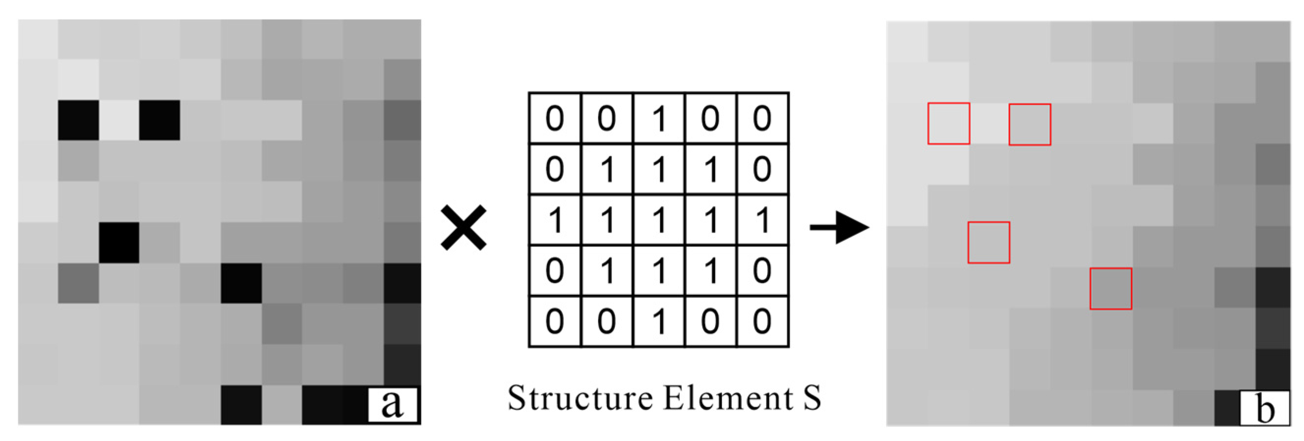
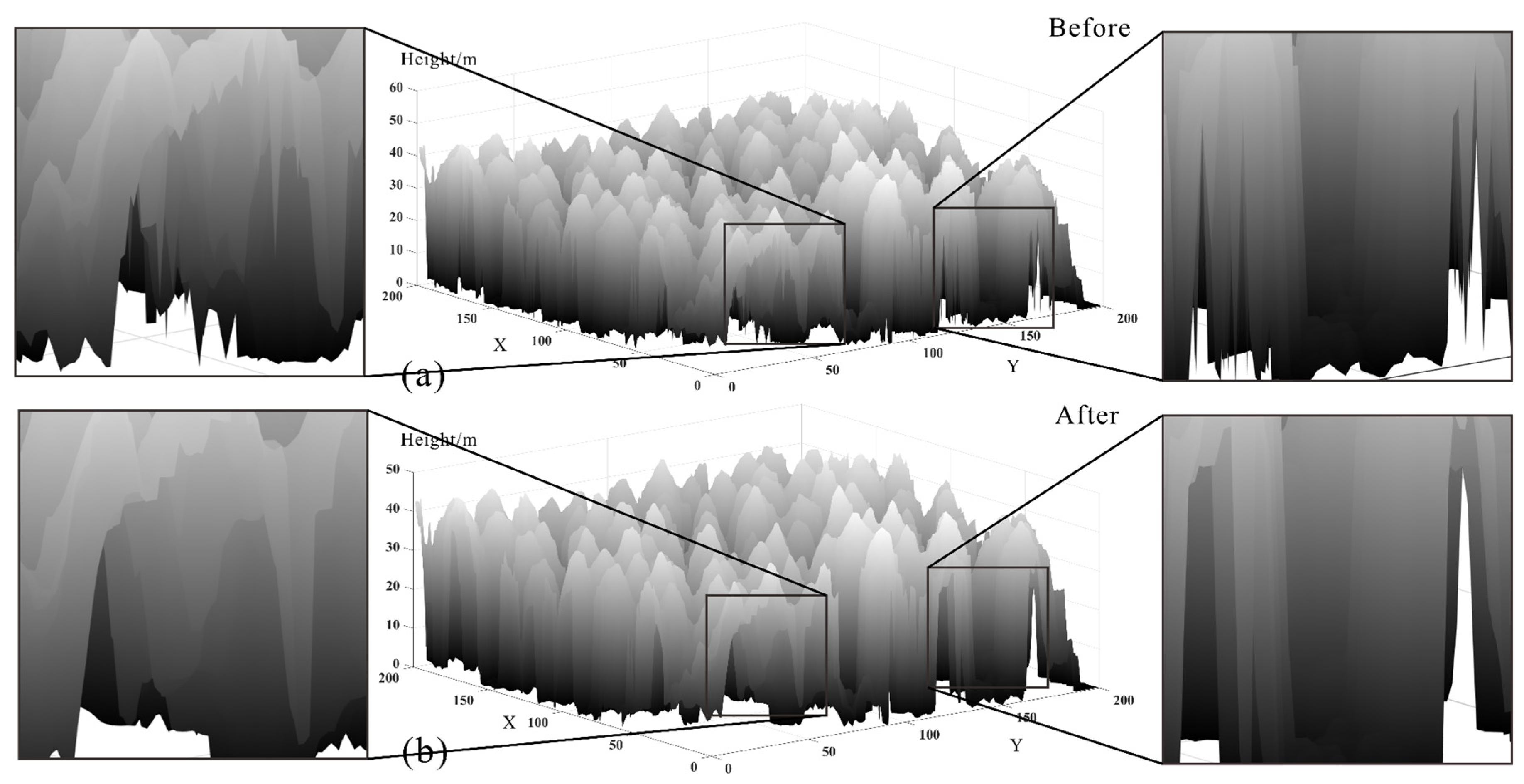
2.3. Filling the Pits

Once the pits on the crown are found, a reasonable value is needed to fill them; if this value of filling is too large, it may cause misidentification of the treetop and if this value is too small, it will not function to optimize the CHM. To solve this problem, in this paper, we smoothed the canopy height models using median filtering. Using the corresponding value in the median filter instead of the pit value, as follows:

$$C_{(i,j)}^{pits}=C_{(i,j)}^{median}$$

(11)

3. Experiments and Analysis

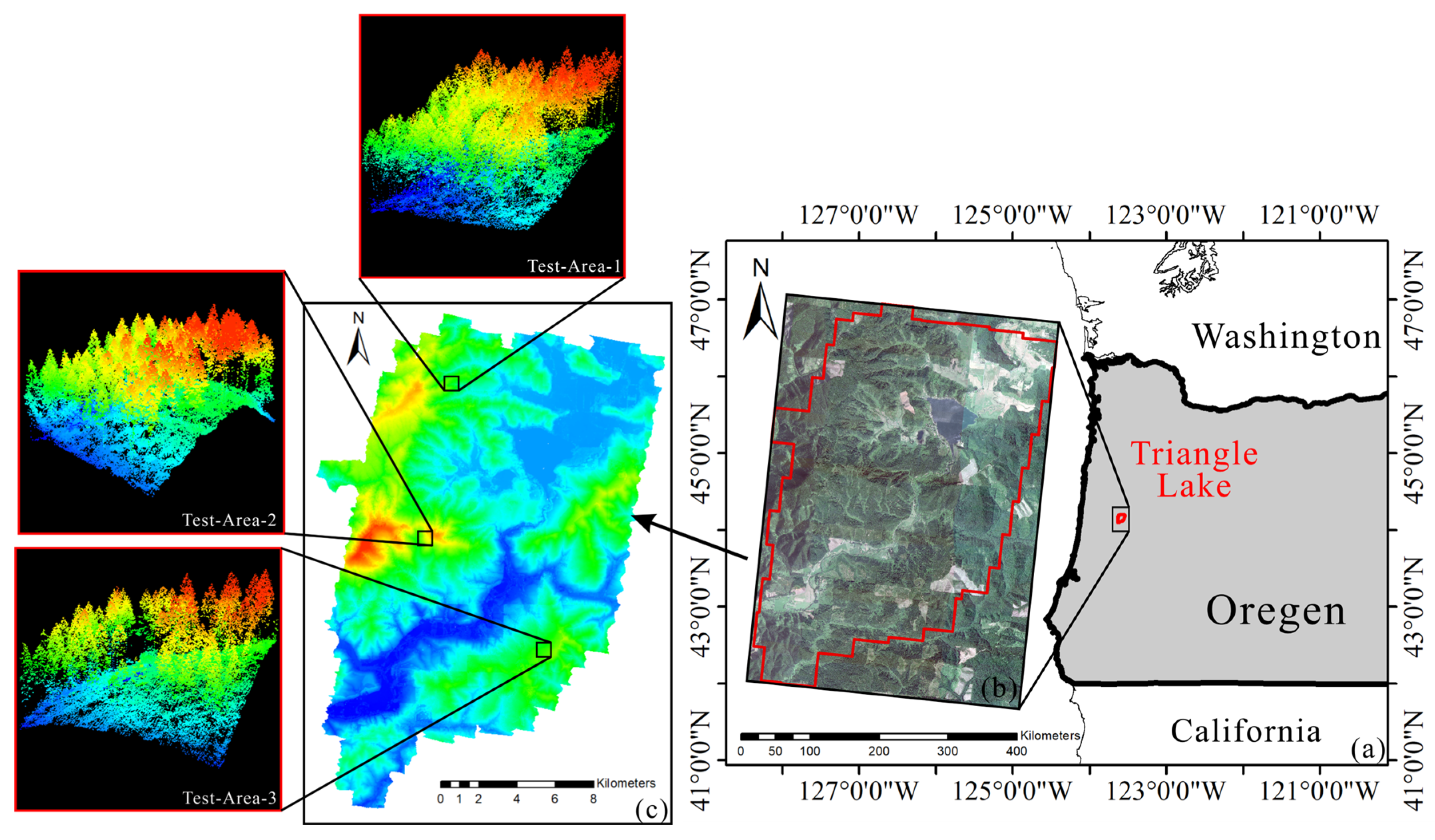
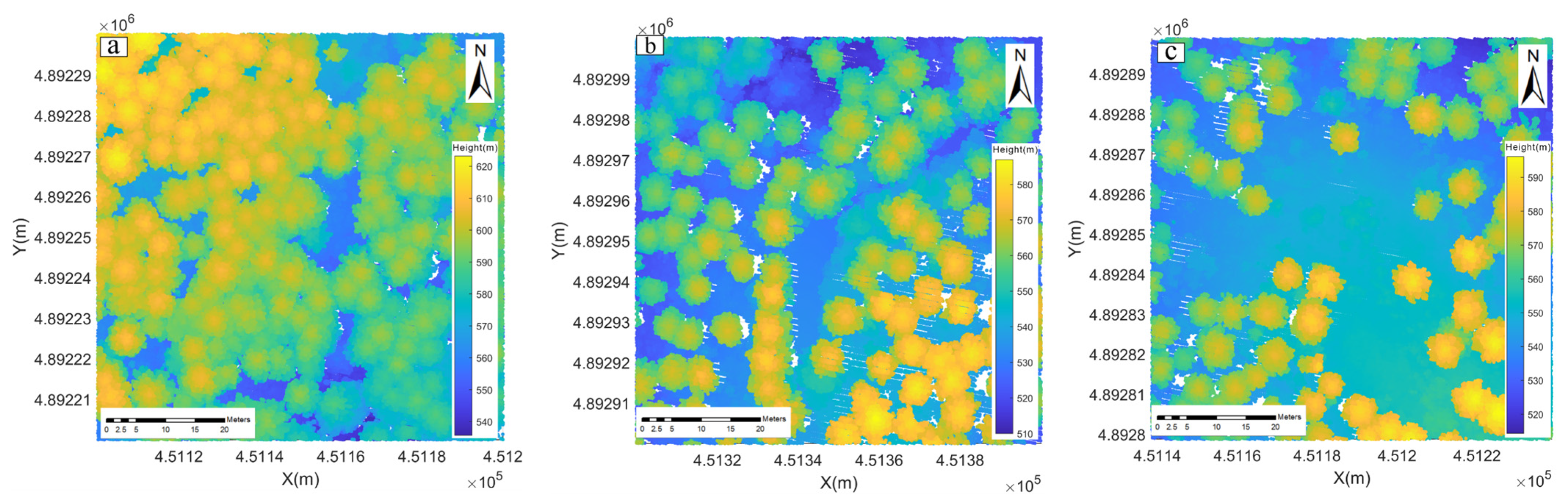
3.1. Experimental Data and Preprocessing

3.1.1. LiDAR Data

In this paper, airborne LiDAR point cloud data from Triangle Lake, 38 km west of Oregon on the Pacific coast of the northwestern United States, are used to validate the effectiveness of the methodology, as shown in Figure 5. The study area is a hilly landscape with a ground slope of 0°–58°, and the main tree species are coniferous trees and pines, of which the most important species are fir, hemlock, and red cedar trees. Airborne laser point cloud data were acquired by a Cessna 337 Skymaster civil aircraft carrying an Optech Gemini Airborne Laser Terrain Mapper (ALTM) system. According to the analysis and acquisition of LiDAR data completed by the National Center for Airborne Laser Mapping (NCALM) in 2013 [40] the forest structure in the study area is complex. The data were collected with an average flight speed of 60 m/s, a scan angle of about 30°, and a flight altitude of 600 m. Data contain four echoes and point cloud density of about 14.35 pts/${\mathrm{m}}^2$.

Three test areas were selected to verify our method, as shown in Figure 6. Each test area is a square with 100 × 100 m². Due to the difficulty of obtaining accurate field survey data for comparison analysis, the visualization software Cloud Compare v2.13 [41] and ArcGIS10.6.1 were used to manually extract the reference treetop data and were recorded as the reference tree heights, which are used for evaluating the performance of the method proposed in this paper [42,43,44]. The characteristics of the reference data are listed in

Table 1. The reference data extracted manually from the study area.

Test Area	Number of Trees	Tree Height(m)		$\mathbf{Point} \mathbf{Density} (\mathbf{pts}/{\mathbf{m}}^2$)
		Average of Height	Std of Height
1	191	43.39	5.28	16.02
2	104	36.32	4.53	13.18
3	75	35.92	6.69	11.64

.

Three test areas to verify the advantages and superiority of method proposed in this paper. Three test areas differed in stem density, with test area 1 having the highest, test area 3 the lowest, and test area 2 being in between. A higher stem density means that the lower and middle trees are more heavily shaded, and some of the lower canopy may be too shaded to be observed. The experiment was carried out in MATLAB R2020b using an Intel (R) Core (TM) i7-4710MQ CPU with the memory of 8 GB. The processing time was 3 min and 10.4 s.

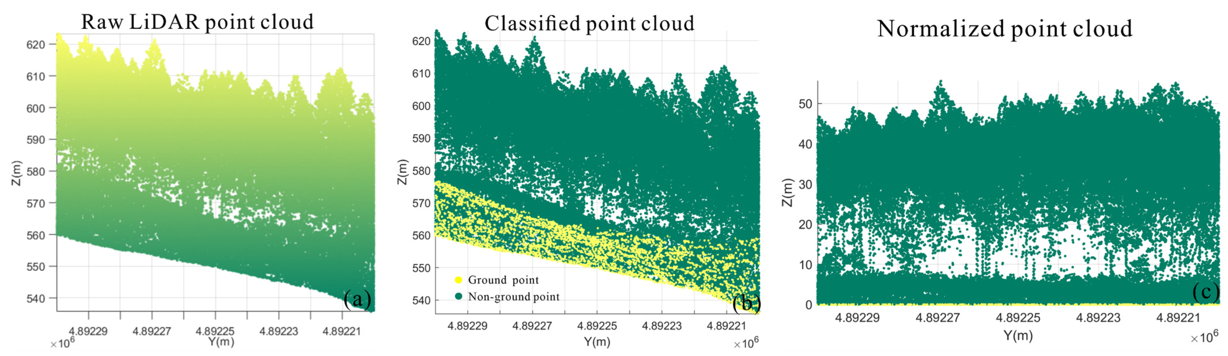
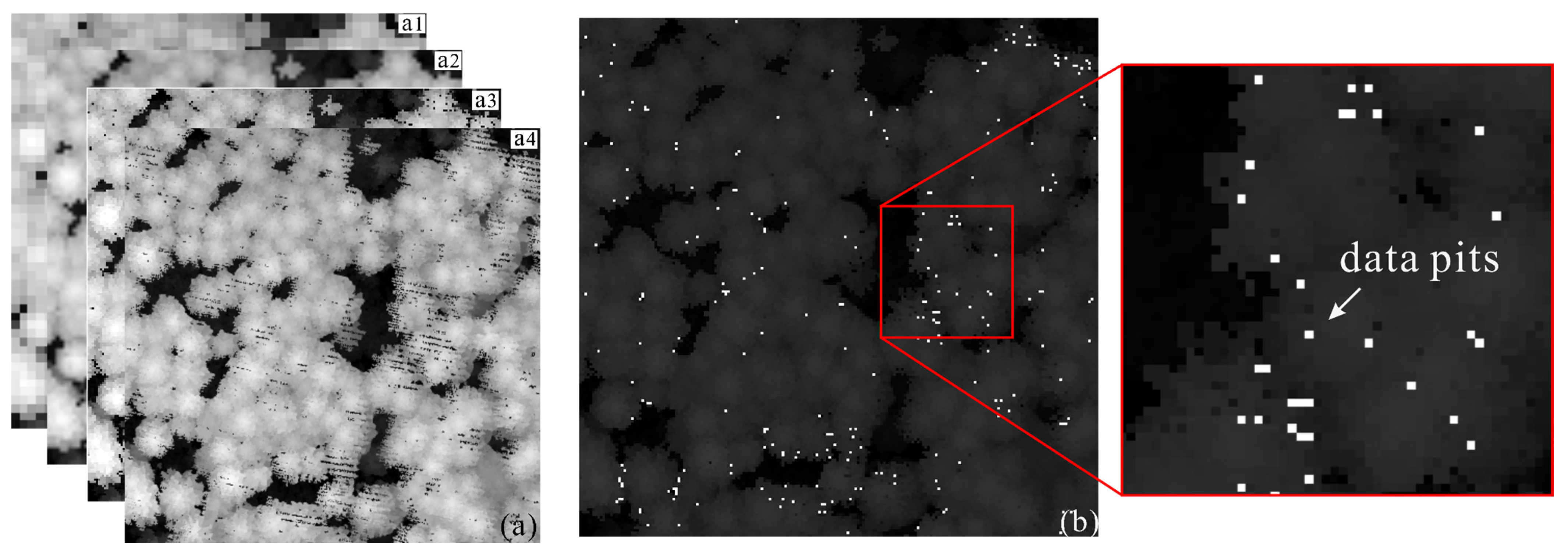
3.1.2. Data Preprocessing

Two main methods were applied to generate CHM from laser point cloud data: one was to obtain the difference between the canopy surface model DSM (digital surface model) and the ground digital elevation model DEM (digital elevation model) and the other is to use the classified ground points to normalize the elevation of the point cloud data, and to then obtain the CHM from the rasterization [45]. In this paper, we directly rasterize the normalized point cloud to generate CHM (as shown in Figure 7), which aims to reduce the loss of canopy information as interpolated only once. Figure 8 shows the CHM raster images at different resolutions. What can be observed is that the data pits issue becomes increasingly obvious as the spatial resolution gradually increases. The classification of ground points was performed using TerraSolidV13 software, and then the height normalization was completed by subtracting the height value of the nearest ground point found from the height value of each non-ground point. Considering the influence of point cloud density and canopy crown width of the survey area on the CHM resolution [36], inverse distance weight (IDW) method [46,47] are used for the normalized point cloud to generate CHMs with spatial resolutions of 2.0 m, 1.0 m, 0.5 m, and 0.25 m for subsequent operations.

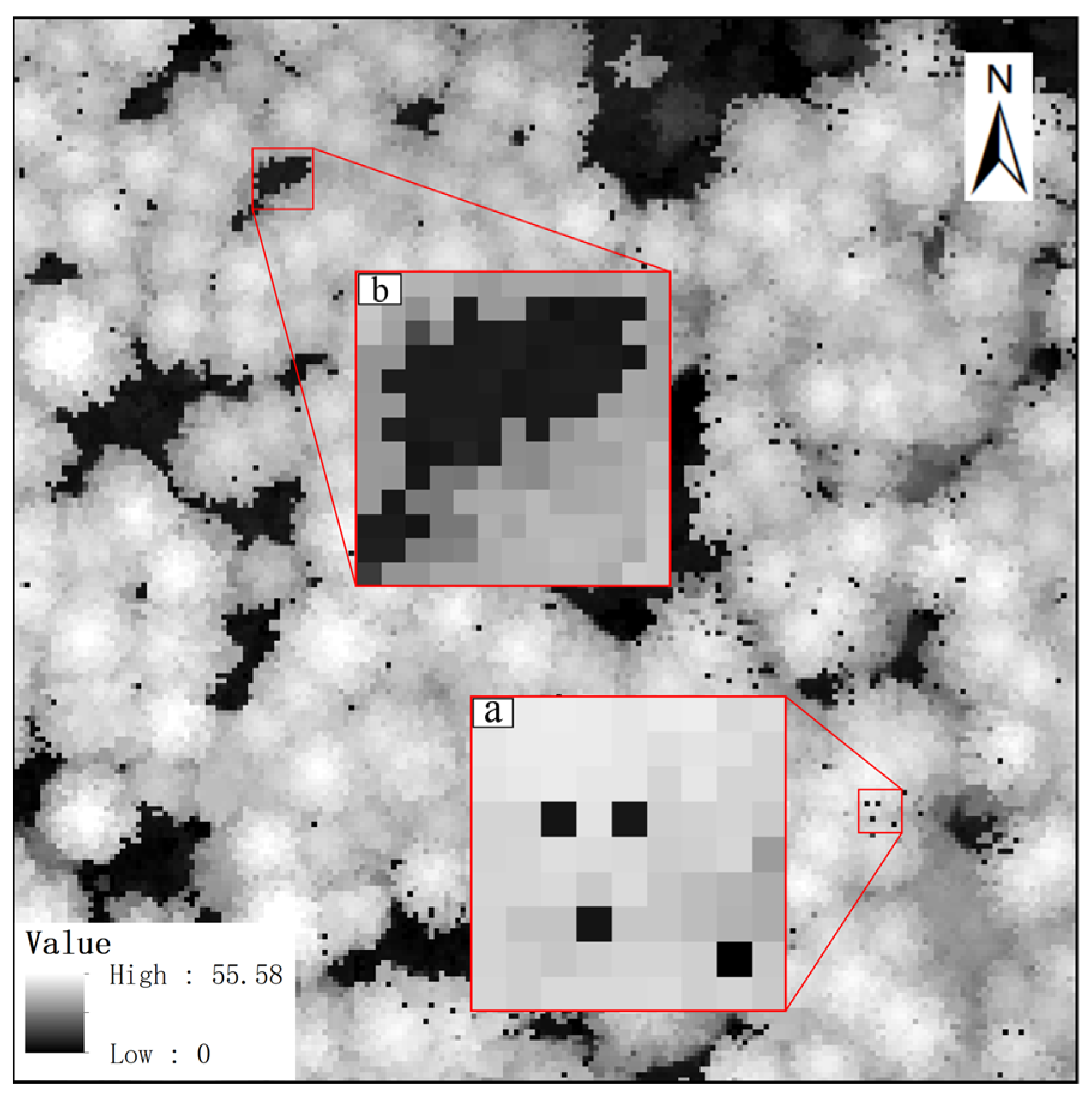
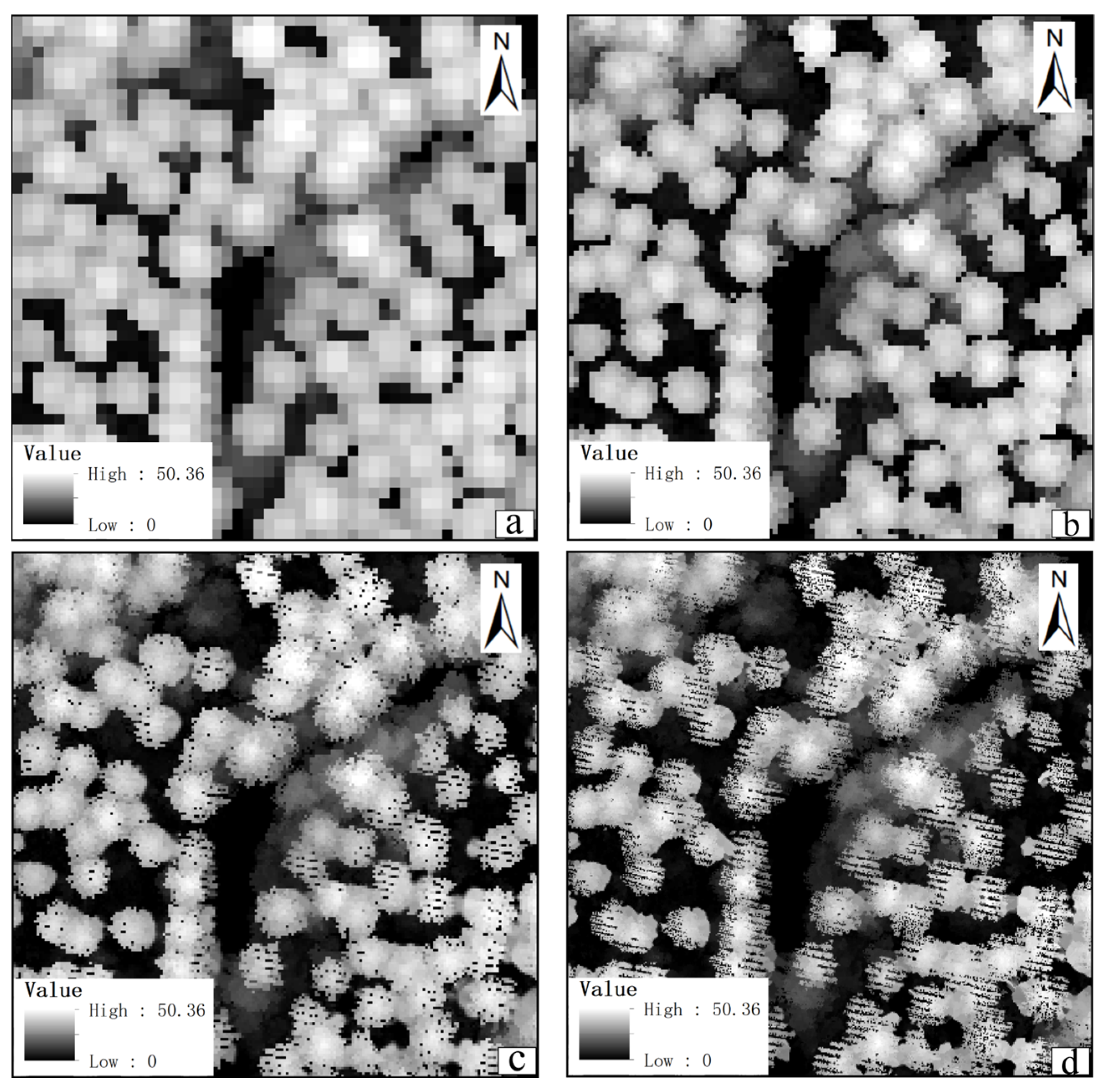
3.2. Automatically Identifying and Filling Pits Pixels for CHM

(1)

Experiment with Test Area 1

The automatic filling pits pixel for CHM is finished through the following 3 steps.

Step 1: Extracting two characteristic parameters, GI and ZV, for canopy pit recognition. Applying the weighted differential gradient method can extract them, and since the extraction process is an automated computation between image pixels, this step does not require human input parameters, Figure 9 shows the extraction results of test area 1.

As shown in Figure 9, when a 3 × 3 window centered on the pit pixel on the CHM image is moved, the characteristic parameters of the neighboring pixels can be computed using Equations (1) and (2). The values of the window are c1 = 41.49, c2 = 42.5, c3 = 43.22, c4 = 42, c5 = 6.5, c6 = 43.07, c7 = 40.68, c8 = 42.43, and c9 = 43.29. The gradients for the pixels within the window can be calculated using Equation (8), i.e., d1 = 2.125, d2 = 1.711, d3 = 1.157, d4 = 1.849, d5 = 4.2, d6 = 0.778, d7 = 3.8, and d8 = 2.56. The gradient weights of the pixels are determined using Equations (5) and (6), i.e., w1 = 8.37, w2 = 5.53, w3 = 3.17, w4 = 6.35, w5 = 66.36, w6 = 2.18, w7 = 44.92, and w8 = 13, and then the gradient weights are assigned to the corresponding neighborhoods pixels for calculating GI, while the ZV is calculated from the median and median absolute deviation within the window. Similarly, the characteristic parameters of the other test areas can be calculated as well.

Step 2: Calculating the canopy constraint to distinguish either canopy gaps or pit pixels. Considering that canopies with different crown widths can be searched, CHMs at different resolutions, whose spatial resolution size should be lower than half of the crown width are merged. Secondly, the CHM with spatial resolutions of 0.25 m, 0.5 m, 1.0 m, and 2.0 m are subjected to the operation using Equation (10), and the weight K in the fusion process is set to 0.25, 0.5, 0.125, and 0.125, respectively, on the basis of the several trial-and-error experimental attempts. Finally, the pit pixels on canopy were distinguished according to Equation (8). The filtered canopy pit pixels are displayed in Figure 10. As can be seen in Figure 10b, our method is able to distinguish the pits from the canopy gaps well in the high stem density area and thus can improve the accuracy of the canopy pit filling.

Step 3. The process of filling pits is finished by replacing the values of these pit pixels with local median values. Figure 11 shows the comparison between before and after filling of the pits for test area 1. From the 3D CHM, it can be seen that the canopy structure information is incomplete before pit filling (Figure 11a), but the overall CHM becomes smoother after pit filling (Figure 11b).

(2)

Experiment with Test Area 2 and Test Area 3

Similar operations were carried out for test area 2 and test area 3. The results of the extracted two characteristic parameters, GI and ZV, for canopy pit recognition are depicted in Figure 12 for test area 2 and in Figure 13 for test area 3.

Also, the same operations for discrimination of the pit pixels on canopy were carried out; the results are depicted in Figure 14 and Figure 15.

Finally, the operation of filling the pits is similar to the one above. The results are shown in Figure 16 for test area 2 and Figure 17 for test area 3.

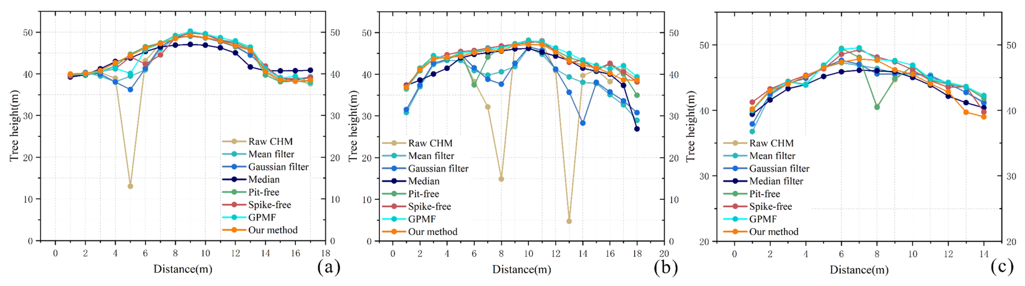
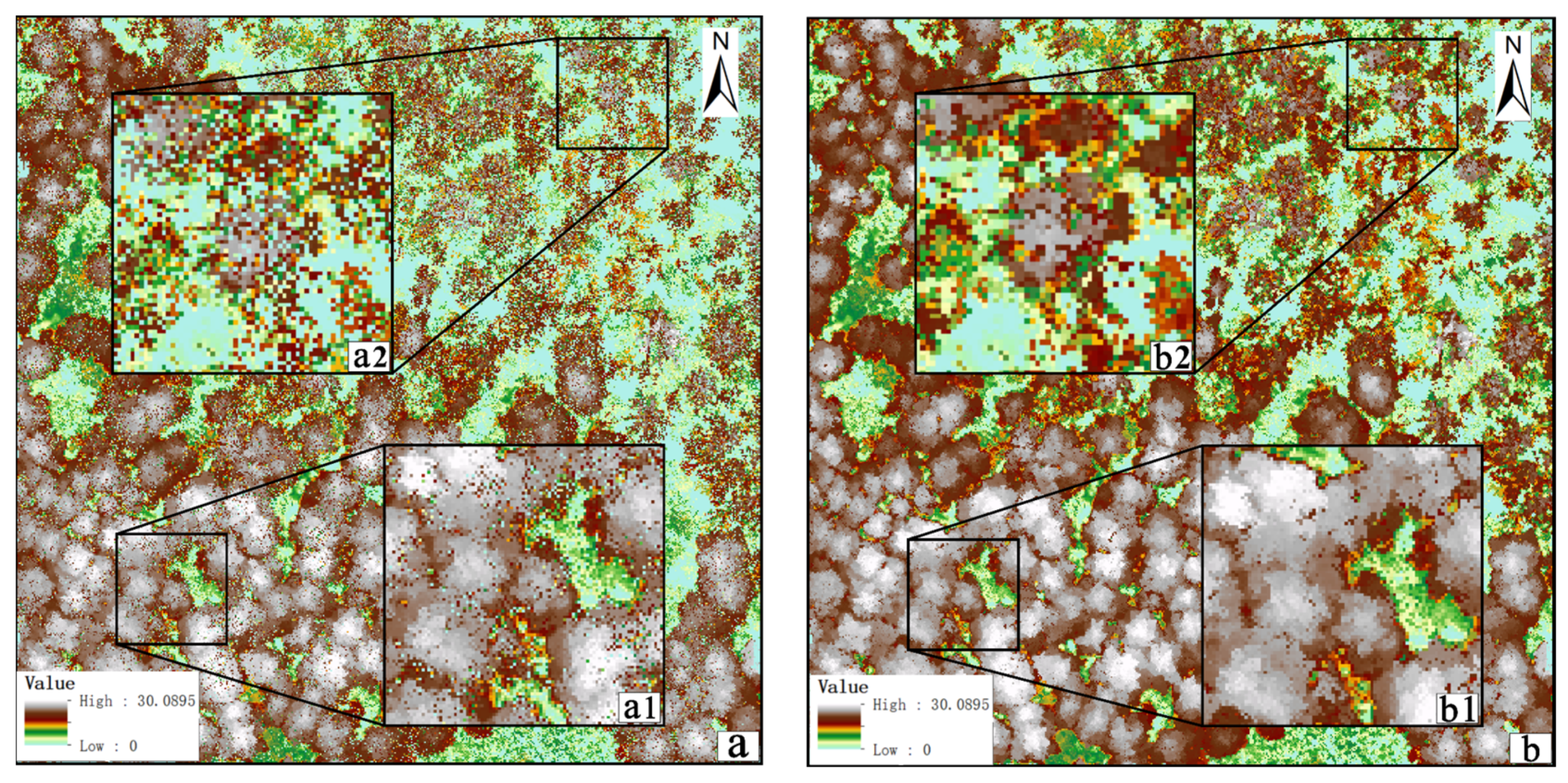
3.3. Comparison and Analysis

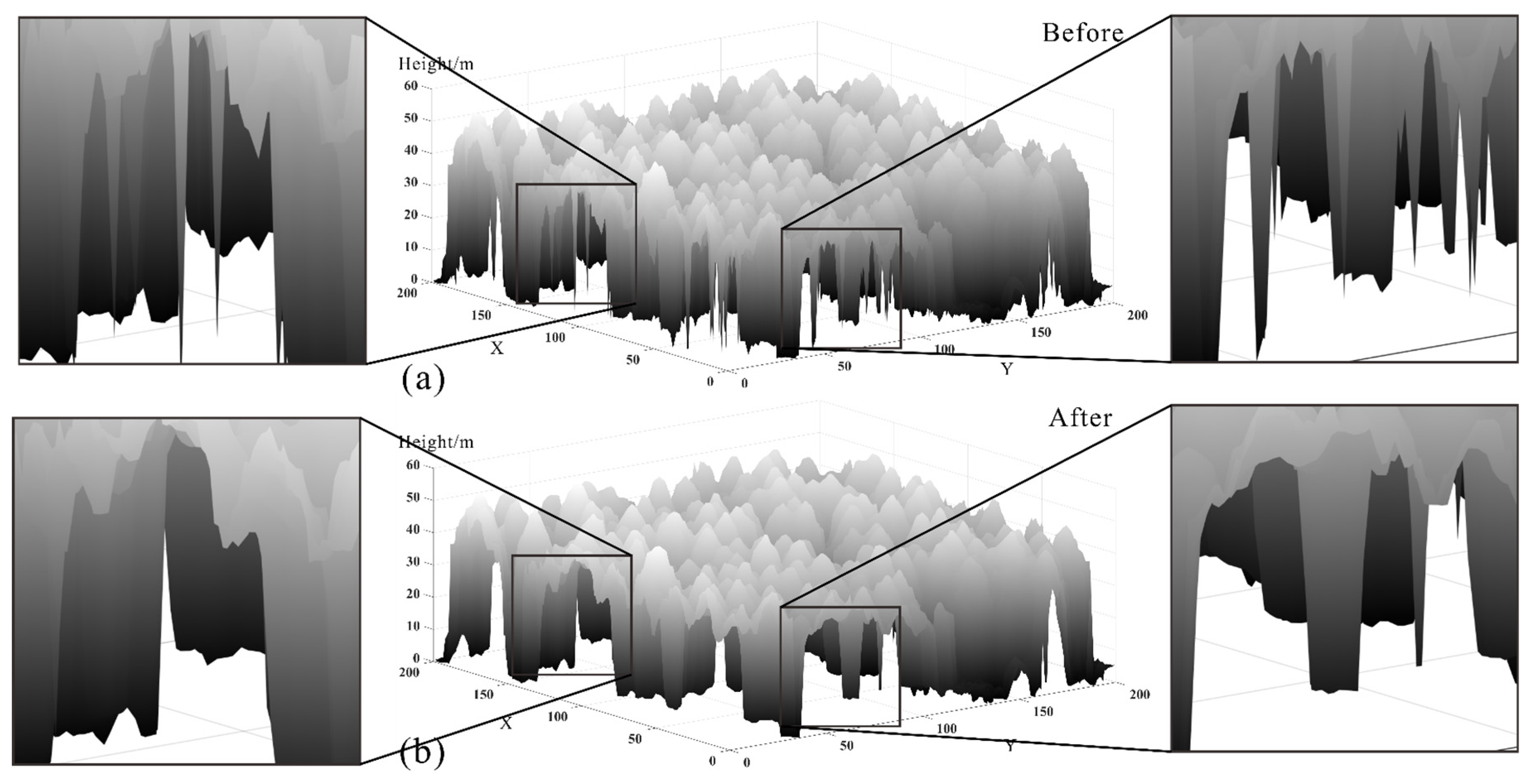
3.3.1. Visual Evaluation

The CHM created before and after processing was visually compared, which is the most direct way to compare the quality of the canopy height model, since a high-quality canopy height model should have no or few pits on the canopy.

The pit-filling results of the different algorithms were visually compared; they can be visually compared from a view of the local canopy. We selected the local canopies of different results, as shown in Figure 18, Figure 19 and Figure 20. On the raw CHM (Figure 18(a1), Figure 19(a1) and Figure 20(a1)), it can be seen that the pixel distribution of pits on the surface of the canopy is inhomogeneous. After the pit-filling process, the surface of the canopy in CHM becomes smoother, but there are differences in the performance of different methods. The median filter is effective in filling data pits but the CHM is over smoothed, causing the edges of the canopy to become blurred. In contrast to the other two window filtering algorithms, the data pits smoothed by the Gaussian and mean filters are too blurred and not well filled. The pit-free algorithm removes most of the pits but in the lower part of the canopy the pits do not seem to be well filled. GPMF and our method have the best performances of all the methods, followed by the spike-free algorithm.

Comparing the experimental results of the three different test areas, the performance of the window filter algorithms is not sensitive to the sparseness of the canopy as the mean, Gaussian, and median are global filters. Their performances in filling data pits are thus not improved. The pit-free algorithm performed better in the dense canopy plot than in the sparse plots, which may be due to the poor pit-filling ability for a single threshold for the lower and middle canopy. The spike-free algorithm, GPMF, and our method have better performance and fill almost all the pits on the surface of the canopy. This was similar to global filtering and performs well in CHMs with different sparsity levels. Figure 21 shows a 0.5 m wide canopy profile that we used to compare the effects of different methods of pit filling. The canopy on the raw CHM showed height anomalies, while the CHM processed by pit-filling algorithm has a profile that is closer to the real shape of the tree crown. Compared with the results of other methods, our method is better to keep the original canopy structure and edge information while filling data pits. Despite the reduced canopy density, our method is still effective for pit filling.

3.3.2. Quantitative Evaluation

This paper introduces root-mean-square error (RMSE), mean bias error (MBE), and coefficient of determination (R²) metrics for quantitatively evaluating the quality of the CHMs created before and after filling pits [48]. The formulae are as follows:

$$RMSE=\sqrt{\frac{{\displaystyle \sum _{i=1}^n{\left(x_i-{\widehat{x}}_i\right)}^2}}{\mathrm{n}}}$$

(12)

$$MBE=\frac{{\displaystyle \sum _{i=1}^n\left(x_i-{\widehat{x}}_i\right)}}{n}$$

(13)

$$R^2=1-\frac{{\displaystyle \sum _{i=1}^n{\left(x_i-{\widehat{x}}_i\right)}^2}}{{\displaystyle \sum _{i=1}^n{\left(x_i-{\overline{x}}_i\right)}^2}}$$

(14)

where n represents the number of observation objects, i.e., the number of pixels involved in the processing; $x_i$ is the true height of the observation object; ${\widehat{x}}_i$ is the height of the observation object after processing; and ${\overline{x}}_i$ is the mean of the observation object.

The results are shown in

Table 2. The height difference of CHMs from the different methods relative to the reference data.

	Methods	Evaluation Parameters
		R2	RMSE	MBE
Test Area 1	Raw CHM	0.79	1.30	1.20
	Mean filter	0.83	1.17	0.62
	Gaussian filter	0.87	1.05	0.88
	Median filter	0.92	0.67	0.48
	Pit free	0.94	0.70	0.28
	Spike free	0.98	0.37	0.16
	GPMF	0.98	0.30	0.13
	Our method	0.99	0.29	0.06
Test Area 2	Raw CHM	0.72	1.48	1.40
	Mean filter	0.78	1.31	1.00
	Gaussian filter	0.76	1.36	0.77
	Median filter	0.89	1.12	0.53
	Pit free	0.86	1.05	0.60
	Spike free	0.98	0.41	0.16
	GPMF	0.98	0.33	0.13
	Our method	0.98	0.31	0.12
Test Area 3	Raw CHM	0.80	1.17	1.54
	Mean filter	0.87	1.08	0.94
	Gaussian filter	0.89	1.00	0.79
	Median filter	0.92	0.88	0.56
	Pit free	0.93	0.77	0.44
	Spike free	0.98	0.47	0.14
	GPMF	0.99	0.30	0.18
	Our method	0.98	0.36	0.12

. The CHM processed changes from the height of the reference because these methods lose information or overestimate the canopy during the calculation process. Window filtering changes the canopy height of CHM, which is related to the fact that they result in over canopy smoothing. The raw CHM is similar to the CHM height after processing with the pit-free algorithm proposed by Ben-Arie (2009) [28], but compared with the reference data, both of them still cause a not-so-small change to the crown height. The spike-free algorithm proposed by Khosravipour (2016) [29] can retain the information of the crown height and edge but it still underestimates the reference data (MBE > 0.1). GPMF and our method perform better, and the changes to the crown height are small (R² close to 1 and RMSE less than 0.4).

To further evaluate the method proposed in this paper, the processed CHMs were applied in individual tree extraction on three test areas. Based on an assumption that the highest point of the canopy is the treetop, local maximum filtering [49], an effective method commonly used in single-tree extraction. Then, the number of extracted single trees are compared with the reference data. Three indicators are introduced to measure the extraction results using the criteria described by Eysn et al. (2015) and others, the rate of trees detected (recall, R), the rate of correct detection (precision P), and precision grade F value (F1 score) [50]. These metrics are defined by the following equations:

$$R=\frac{TP}{TP+FN}\times 100\%$$

(15)

$$P=\frac{TP}{TP+FP}\times 100\%$$

(16)

$$F=2\times \frac{P\times R}{P+R}\times 100\%$$

(17)

where TP is the number of trees correctly detected, FN is the number of trees not detected, and FP is the number of trees incorrectly detected.

Table 3. Accuracy comparison of CHM individual tree extraction after methods processing.

Methods	Indicator	Test Area 1	Test Area 2	Test Area 3
Raw CHM	P	0.69	0.71	0.61
	R	0.75	0.75	0.64
	F1 score	0.72	0.73	0.62
Mean filter	P	0.79	0.79	0.80
	R	0.76	0.75	0.70
	F1 score	0.77	0.77	0.75
Gaussian filter	P	0.79	0.78	0.83
	R	0.78	0.77	0.75
	F1 score	0.78	0.77	0.79
Median filter	P	0.77	0.73	0.76
	R	0.86	0.88	0.89
	F1 score	0.81	0.80	0.82
Pit free	P	0.85	0.86	0.82
	R	0.85	0.87	0.89
	F1 score	0.85	0.86	0.86
Spike free	P	0.86	0.82	0.82
	R	0.85	0.88	0.84
	F1 score	0.85	0.85	0.83
GPMF	P	0.86	0.82	0.87
	R	0.85	0.89	0.92
	F1 score	0.85	0.85	0.89
Our method	P	0.83	0.89	0.89
	R	0.84	0.86	0.93
	F1 score	0.83	0.88	0.91

shows the accuracy of individual tree detection, the average F1 score of our method was 87.3% in three test areas, which was the best performance out of seven other CHMs. The precision and recall of our method were almost the best; however, GPMF was better than our method in test area 1, where trees were dense. In test area 1, the F1 score of spike free and GPMF were higher than our method by 0.02. Our method achieved the best performance in test area 2 and test area 3, with the highest F1 score close to 0.9 out of all methods. These findings illustrate that the CHMs processed by our method overall exhibited good performance in terms of individual tree detection.

The performance of the raw CHM is worst due to the presence of a large number of pits on its canopy surface, so the treetop points were difficult to be detected, resulting in a low F1 score of 70.5%. In window filter algorithms, the F1 score of the median method is better than that of the mean and Gaussian method. The precision and recall of window filters were still low because the over smoothing of the CHMs resulted in blurring the canopy structure and omission of the treetop. In addition, the median filtering algorithm produces many approximations of pixel values on the surface of the canopy, which gives the method a lower precision than that of both mean and Gaussian methods. The pit-free method produced slightly better F1 score than the spike-free method in three test areas.

3.4. Discussion

To demonstrate the advantages of our method in different types of forests over other methods, the experiment in mixed forests was conducted, where the tree species are more diverse (Figure 22). Comparing the results before and after pit filling, it can be demonstrated that our method still performs well for pit filling in CHM, and the filling effect for conifers is better than for other tree species; moreover, our method not only fills pits effectively but also retains the crown edge information better.

This study aims to propose an effective pit-filling approach to enhance the accuracy of CHM. Weighted differential gradient method for filling pits in LiDAR canopy height model can take advantage of the a priori knowledge of forests by using the gradient differential information and robust Z-score values of the canopy as a judgment criterion for pits and adding canopy constraints. Both the gradient index and the robust Z-score value are automated calculation processes and do not need to be considered as added more parameters. The canopy constraint is actually the canopy area, and pixels with canopy gaps are easily misidentified as pits in CHM, which can easily lead to overfilling if they are not distinguished. The method proposed in this paper has been evaluated from both a visual comparison and a quantitative assessment, and the experimental results show that it has good results in CHM pit removal.

4. Conclusions

A pit identification and filling method for the LiDAR canopy height model (CHM) has been proposed in this paper. The proposed method first finds the pits hidden in the CHM and then fills them using the proposed algorithm. This method uses gradient differential information between the pit pixels and their eight neighbors, and the gradient index and Z-score values as criteria to identify the pits in CHM. For a canopy area, the CHMs with different spatial resolutions are merged by using the developed image processing algorithm. The innovation of this study is as follows: (1) The gradient differential information between the pit pixels and their eight neighbors are used to recognize the pits. (2) An image processing algorithm is proposed to merge the CHMs with different spatial resolutions.

To evaluate the performance of the method proposed in this paper, the experiments and analyses were conducted in three coniferous test areas with different forest conditions. The verified results demonstrated that the method proposed in this paper has good results in removing the pits and retains the structural details of the canopy well. The method reaches an average RMSE of 0.32 m and the average bias of 0.12 m. In addition, the method proposed in this paper also outperforms the other methods in terms of treetop detection, with an average F1 score of 87.8%. Therefore, it can be concluded that the method proposed in this paper can effectively fill the pitted points and has largely improved the accuracy of CHM.

However, the proposed model still requires improvement in the future. For example, the construction of canopy constraints requires a fusion of CHMs with different spatial resolutions, and the setting of the weights for fusion still relies on manual judgment. Therefore, our future work will focus on parameter adaptivity and improving the universality of the method.

References

1. Kim, D.H.; Ko, C.U.; Kim, D.G.; Kang, J.T.; Park, J.M.; Cho, H.J. Automated Segmentation of Individual Tree Structures Using Deep Learning over LiDAR Point Cloud Data. Forests 2023, 14, 1159. [Google Scholar] [CrossRef]
2. Whelan, A.W.; Cannon, J.B.; Bigelow, S.W.; Rutledge, B.T.; Meador, A.J.S. Improving generalized models of forest structure in complex forest types using area-and voxel-based approaches from lidar. Remote Sens. Environ. 2023, 284, 113362. [Google Scholar] [CrossRef]
3. Oehmcke, S.; Li, L.; Trepekli, K.; Revenga, J.C.; Nord-Larsen, T.; Gieseke, F.; Igel, C. Deep point cloud regression for above-ground forest biomass estimation from airborne LiDAR. Remote Sens. Environ. 2024, 302, 113968. [Google Scholar] [CrossRef]
4. Zhu, X.; Liu, J.; Skidmore, A.K.; Premier, J.; Heurich, M. A voxel matching method for effective leaf area index estimation in temperate deciduous forests from leaf-on and leaf-off airborne LiDAR data. Remote Sens. Environ. 2020, 240, 111696. [Google Scholar] [CrossRef]
5. Schneider, F.D.; Kükenbrink, D.; Schaepman, M.E.; Schimel, D.S.; Morsdorf, F. Quantifying 3D structure and occlusion in dense tropical and temperate forests using close-range LiDAR. Agric. For. Meteorol. 2019, 268, 249–257. [Google Scholar] [CrossRef]
6. Liu, Q.; Fu, L.; Wang, G.; Li, S.; Li, Z.; Chen, E.; Hu, K. Improving estimation of forest canopy cover by introducing loss ratio of laser pulses using airborne LiDAR. IEEE Trans. Geosci. Remote Sens. 2019, 58, 567–585. [Google Scholar] [CrossRef]
7. Cai, S.; Zhang, W.; Jin, S.; Shao, J.; Li, L.; Yu, S.; Yan, G. Improving the estimation of canopy cover from UAV-LiDAR data using a pit-free CHM-based method. Int. J. Digit. Earth 2021, 14, 1477–1492. [Google Scholar] [CrossRef]
8. Tian, Y.; Huang, H.; Zhou, G.; Zhang, Q.; Tao, J.; Zhang, Y.; Lin, J. Aboveground mangrove biomass estimation in Beibu Gulf using machine learning and UAV remote sensing. Sci. Total Environ. 2021, 781, 146816. [Google Scholar] [CrossRef]
9. Zhao, K.; Suarez, J.C.; Garcia, M.; Hu, T.; Wang, C.; Londo, A. Utility of multitemporal lidar for forest and carbon monitoring: Tree growth, biomass dynamics, and carbon flux. Remote Sens. Environ. 2018, 204, 883–897. [Google Scholar] [CrossRef]
10. Qi, Z.; Li, S.; Pang, Y.; Zheng, G.; Kong, D.; Li, Z. Assessing spatiotemporal variations of forest carbon density using bi-temporal discrete aerial laser scanning data in Chinese boreal forests. For. Ecosyst. 2023, 10, 100135. [Google Scholar] [CrossRef]
11. Hao, J.; Li, X.; Wu, H.; Yang, K.; Zeng, Y.; Wang, Y.; Pan, Y. Extraction and analysis of tree canopy height information in high-voltage transmission-line corridors by using integrated optical remote sensing and LiDAR. Geod. Geodyn. 2023, 14, 292–303. [Google Scholar] [CrossRef]
12. Erfanifard, Y.; Stereńczak, K.; Kraszewski, B.; Kamińska, A. Development of a robust canopy height model derived from ALS point clouds for predicting individual crown attributes at the species level. Int. J. Remote Sens. 2018, 39, 9206–9227. [Google Scholar] [CrossRef]
13. Xiao, C.; Qin, R.; Huang, X. Treetop detection using convolutional neural networks trained through automatically generated pseudo labels. Int. J. Remote Sens. 2020, 41, 3010–3030. [Google Scholar] [CrossRef]
14. Mu, Y.; Zhou, G.; Wang, H. Canopy lidar point cloud data k-means clustering watershed segmentation method. ISPRS Annals of the Photogrammetry. Remote Sens. Spat. Inf. Sci. 2020, 6, 67–73. [Google Scholar] [CrossRef]
15. Estornell, J.; Hadas, E.; Martí, J.; López-Cortés, I. Tree extraction and estimation of walnut structure parameters using airborne LiDAR data. Int. J. Appl. Earth Obs. Geoinf. 2021, 96, 102273. [Google Scholar] [CrossRef]
16. Liu, H.; Dong, P. A new method for generating canopy height models from discrete-return LiDAR point clouds. Remote Sens. Lett. 2014, 5, 575–582. [Google Scholar] [CrossRef]
17. Chang, K.T.; Lin, C.; Lin, Y.C.; Liu, J.K. Accuracy Assessment of Crown Delineation Methods for the Individual Trees Using LIDAR Data. Int. Arch. Photogramm. Remote Sens. Spat. Inf. Sci. 2016, 41, 585–588. [Google Scholar] [CrossRef]
18. Khosravipour, A.; Skidmore, A.K.; Isenburg, M.; Wang, T.; Hussin, Y.A. Generating pit-free canopy height models from airborne lidar. Photogramm. Eng. Remote Sens. 2014, 80, 863–872. [Google Scholar] [CrossRef]
19. Duan, Z.; Zeng, Y.; Zhao, D.; Wu, B.; Zhao, Y.; Zhu, J. Method of removing pits of canopy height model from airborne laser radar. Trans. Chin. Soc. Agric. Eng. 2014, 30, 209–217. [Google Scholar]
20. Zhao, D.; Pang, Y.; Li, Z.; Sun, G. Filling invalid values in a lidar-derived canopy height model with morphological crown control. Int. J. Remote Sens. 2013, 34, 4636–4654. [Google Scholar] [CrossRef]
21. Kucharczyk, M.; Hugenholtz, C.H.; Zou, X. UAV–LiDAR accuracy in vegetated terrain. J. Unmanned Veh. Syst. 2018, 6, 212–234. [Google Scholar] [CrossRef]
22. Axelsson, P. DEM generation from laser scanner data using adaptive TIN models. Int. Arch. Photogramm. Remote Sens. 2000, 33, 110–117. [Google Scholar]
23. LaRue, E.A.; Fahey, R.; Fuson, T.L.; Foster, J.R.; Matthes, J.H.; Krause, K.; Hardiman, B.S. Evaluating the sensitivity of forest structural diversity characterization to LiDAR point density. Ecosphere 2022, 13, e4209. [Google Scholar] [CrossRef]
24. Swanson, C.; Merrick, T.; Abelev, A.; Liang, R.; Vermillion, M.; Buma, W.; Li, R. Effects of point density on interpretability of lidar-derived forest structure metrics in two temperate forests. bioRxiv 2024. [Google Scholar] [CrossRef]
25. Shamsoddini, A.; Turner, R.; Trinder, J.C. Improving lidar-based forest structure mapping with crown-level pit removal. J. Spat. Sci. 2013, 58, 29–51. [Google Scholar] [CrossRef]
26. Mielcarek, M.; Stereńczak, K.; Khosravipour, A. Testing and evaluating different LiDAR-derived canopy height model generation methods for tree height estimation. Int. J. Appl. Earth Obs. Geoinf. 2018, 71, 132–143. [Google Scholar] [CrossRef]
27. Barnes, C.; Balzter, H.; Barrett, K.; Eddy, J.; Milner, S.; Suárez, J.C. Individual tree crown delineation from airborne laser scanning for diseased larch forest stands. Remote Sens. 2017, 9, 231. [Google Scholar] [CrossRef]
28. Ben-Arie, J.R.; Hay, G.J.; Powers, R.P.; Castilla, G.; St-Onge, B. Development of a pit filling algorithm for LiDAR canopy height models. Comput. Geosci. 2009, 35, 1940–1949. [Google Scholar] [CrossRef]
29. Khosravipour, A.; Skidmore, A.K.; Isenburg, M. Generating spike-free digital surface models using LiDAR raw point clouds: A new approach for forestry applications. Int. J. Appl. Earth Obs. Geoinf. 2016, 52, 104–114. [Google Scholar] [CrossRef]
30. Chen, C.; Wang, Y.; Li, Y.; Yue, T.; Wang, X. Robust and parameter-free algorithm for constructing pit-free canopy height models. ISPRS Int. J. Geo-Inf. 2017, 6, 219. [Google Scholar] [CrossRef]
31. Hao, Y.; Zhen, Z.; Li, F.; Zhao, Y. A graph-based progressive morphological filtering (GPMF) method for generating canopy height models using ALS data. Int. J. Appl. Earth Obs. Geoinf. 2019, 79, 84–96. [Google Scholar] [CrossRef]
32. Rousseeuw, P.J.; Hubert, M. Robust statistics for outlier detection. Wiley Interdiscip. Rev. Data Min. Knowl. Discov. 2011, 1, 73–79. [Google Scholar] [CrossRef]
33. Zhang, W.; Cai, S.; Liang, X.; Shao, J.; Hu, R.; Yu, S.; Yan, G. Cloth simulation-based construction of pit-free canopy height models from airborne LiDAR data. For. Ecosyst. 2020, 7, 1. [Google Scholar] [CrossRef]
34. Song, Q.; Xiang, M.; Hovis, C.; Zhou, Q.; Lu, M.; Tang, H.; Wu, W. Object-based feature selection for crop classification using multi-temporal high-resolution imagery. Int. J. Remote Sens. 2019, 40, 2053–2068. [Google Scholar] [CrossRef]
35. Liu, L.; Lim, S.; Shen, X.; Yebra, M. A multiscale morphological algorithm for improvements to canopy height models. Comput. Geosci. 2019, 130, 20–31. [Google Scholar] [CrossRef]
36. Yin, D.; Wang, L. Individual mangrove tree measurement using UAV-based LiDAR data: Possibilities and challenges. Remote Sens. Environ. 2019, 223, 34–49. [Google Scholar] [CrossRef]
37. Qiao, L.; Gao, D.; Zhao, R.; Tang, W.; An, L.; Li, M.; Sun, H. Improving estimation of LAI dynamic by fusion of morphological and vegetation indices based on UAV imagery. Comput Electron Agr. 2022, 192, 106603. [Google Scholar] [CrossRef]
38. Holmgren, J.; Lindberg, E.; Olofsson, K.; Persson, H.J. Tree crown segmentation in three dimensions using density models derived from airborne laser scanning. Int. J. Remote Sens. 2022, 43, 299–329. [Google Scholar] [CrossRef]
39. Rizaev, I.G.; Pogorelov, A.V.; Krivova, M.A. A technique to increase the efficiency of artefacts identification in lidar-based canopy height models. Int. J. Remote Sens. 2016, 37, 1658–1670. [Google Scholar] [CrossRef]
40. Marshall, J.A.; Roering, J.J.; Gavin, D.G.; Granger, D.E. Late Quaternary Climatic Controls on Erosion Rates and Geomorphic Processes in Western Oregon, USA. Geol. Soc. Am. Bull. 2017, 129, 715–731. [Google Scholar] [CrossRef]
41. Cloud Compare. Available online: http://www.cloudcompare.org/main.html (accessed on 25 March 2022).
42. Zhen, Z.; Quackenbush, L.J.; Zhang, L. Impact of tree-oriented growth order in marker-controlled region growing for individual tree crown delineation using airborne laser scanner (ALS) data. Remote Sens. 2014, 6, 555–579. [Google Scholar] [CrossRef]
43. Zhen, Z.; Quackenbush, L.J.; Stehman, S.V.; Zhang, L. Agent-based region growing for individual tree crown delineation from airborne laser scanning (ALS) data. Int. J. Remote Sens. 2015, 36, 1965–1993. [Google Scholar] [CrossRef]
44. Granholm, A.H.; Lindgren, N.; Olofsson, K.; Nyström, M.; Allard, A.; Olsson, H. Estimating vertical canopy cover using dense image-based point cloud data in four vegetation types in southern Sweden. Int. J. Remote Sens. 2017, 38, 1820–1838. [Google Scholar] [CrossRef]
45. Oh, S.; Jung, J.; Shao, G.; Shao, G.; Gallion, J.; Fei, S. High-resolution canopy height model generation and validation using USGS 3DEP LiDAR data in Indiana, USA. Remote Sens. 2022, 14, 935. [Google Scholar] [CrossRef]
46. Chen, G.; Zhao, K.; McDermid, G.J.; Hay, G.J. The influence of sampling density on geographically weighted regression: A case study using forest canopy height and optical data. Int. J. Remote Sens. 2012, 33, 2909–2924. [Google Scholar] [CrossRef]
47. Zhou, G.; Song, B.; Liang, P.; Xu, J.; Yue, T. Voids filling of DEM with multiattention generative adversarial network model. Remote Sens. 2022, 14, 1206. [Google Scholar] [CrossRef]
48. Quan, Y.; Li, M.; Hao, Y.; Wang, B. Comparison and evaluation of different pit-filling methods for generating high resolution canopy height model using UAV laser scanning data. Remote Sens. 2021, 13, 2239. [Google Scholar] [CrossRef]
49. Bonnet, S.; Lisein, J.; Lejeune, P. Comparison of UAS photogrammetric products for tree detection and characterization of coniferous stands. Int. J. Remote Sens. 2017, 38, 5310–5337. [Google Scholar] [CrossRef]
50. Eysn, L.; Hollaus, M.; Lindberg, E.; Berger, F.; Monnet, J.M.; Dalponte, M.; Pfeifer, N. A benchmark of lidar-based single tree detection methods using heterogeneous forest data from the alpine space. Forests 2015, 6, 1721–1747. [Google Scholar] [CrossRef]
Figure 1. The flowchart of the proposed method.
Remotesensing 16 01304 g001
Figure 2. A pit pixel with its eight neighborhoods: (a) canopy of a tree and (b) a pit pixel.
Remotesensing 16 01304 g002
Figure 3. Canopy height model with a resolution of 0.5 m: (a) pits and (b) canopy gaps.
Remotesensing 16 01304 g003
Figure 4. Morphologic closure operation for raw CHM image: (a) raw CHM; (b) processed CHM.
Remotesensing 16 01304 g004
Figure 5. Study area located in Triangle Lake, Oregon, USA: (a) map of study area; (b) study area coverage; and (c) the three selected test areas.
Remotesensing 16 01304 g005
Figure 6. Three test areas with trees of different heights and stem densities: (a) is the test area 1, (b) represents the test area 2, and (c) represents test area 3.
Remotesensing 16 01304 g006
Figure 7. The LiDAR point cloud data preprocessing: (a) raw LiDAR point cloud data, (b) classified point cloud data, and (c) normalized point cloud data.
Remotesensing 16 01304 g007
Figure 8. CHM at different spatial resolutions: (a) is with 2.0 m spatial resolution; (b) is 1.0 m spatial resolution; (c) is with 0.5 m spatial resolution; and (d) is with 0.25 m spatial resolution.
Remotesensing 16 01304 g008
Figure 9. Extraction of characteristic parameters: (a) CHM, (b) GI, and (c) ZV; (a1c1) zoom display; (a2c2) pixel values in the window.
Remotesensing 16 01304 g009
Figure 10. (a) The merging CHMs with different spatial resolutions, where (a) represents a merged images at 2.0 m (a1), 1.0 m (a2), 0.5 m (a3), 0.25 m (a4); (b) represents the distinguished canopy pit pixels.
Remotesensing 16 01304 g010
Figure 11. The CHMs of test area 1: (a) before pit filling and (b) after pit filling.
Remotesensing 16 01304 g011
Figure 12. Extraction of characteristic parameters for test area 2. (a) CHM, (b) GI, and (c) ZV.
Remotesensing 16 01304 g012
Figure 13. The extracted characteristic parameters for test area 3. (a) CHM, (b) GI, and (c) ZV.
Remotesensing 16 01304 g013
Figure 14. Merging CHMs with different spatial resolutions: (a) represents a merged image at 2.0 m (a1), 1.0 m (a2), 0.5 m (a3), 0.25 m (a4); (b) represents the distinguished canopy pit pixels.
Remotesensing 16 01304 g014
Figure 15. Merging CHMs with different spatial resolutions: (a) represents a merged images at 2.0 m (a1), 1.0 m (a2), 0.5 m (a3), 0.25 m (a4); (b) represents the distinguished canopy pit pixels.
Remotesensing 16 01304 g015
Figure 16. The CHMs of test area 2 with (a) before pit filling and (b) after pit filling.
Remotesensing 16 01304 g016
Figure 17. The CHMs of test area 3 with (a) before pit filling and (b) after pit filling.
Remotesensing 16 01304 g017
Figure 18. Comparison analysis between the CHMs with 0.5 m resolution created by six pit-filling algorithms in test area 1: (a) is the original CHM, (b) is from the mean filter method, (c) is from the Gaussian filter, (d) is from the median filter, (e) is from the pit-free algorithm, (f) is from the spike-free algorithm, (g) is from the GPMF algorithm, and (h) is from the method proposed in this paper. (a1h1) zoom display.
Remotesensing 16 01304 g018
Figure 19. Comparison analysis between the CHMs with 0.5 m resolution created by six pit-filling algorithms in test area 2: (a) is the original CHM, (b) is from the mean filter method, (c) is from the Gaussian filter, (d) is from the median filter, (e) is from the pit-free algorithm, (f) is from the spike-free algorithm, (g) is from the GPMF algorithm, and (h) is from the method proposed in this paper. (a1h1) zoom display.
Remotesensing 16 01304 g019
Figure 20. Comparison analysis between the CHMs with 0.5 m resolution created by six pit-filling algorithms in test area 3: (a) is the original CHM, (b) is from the mean filter method, (c) is from the Gaussian filter, (d) is from the median filter, (e) is from the pit-free algorithm, (f) is from the spike-free algorithm, (g) is from the GPMF algorithm, and (h) is from the method proposed in this paper. (a1h1) zoom display.
Remotesensing 16 01304 g020
Figure 21. The profile for comparison analysis of six methods with a localized single tree at the three test areas: (a) test area 1, (b) test area 2, (c) test area 3.
Remotesensing 16 01304 g021
Figure 22. Comparison between the CHM in mixed forest: (a) the raw CHM and (b) the filled CHM using our method: (a1,a2) zoom display for raw CHM, (b1,b2) zoom display for filled CHM.
Remotesensing 16 01304 g022