Comparison of Cloud-Mask Algorithms and Machine-Learning Methods Using Sentinel-2 Imagery for Mapping Paddy Rice in Jianghan Plain

Abstract

Southern China, one of the traditional rice production bases, has experienced significant declines in the area of rice paddy since the beginning of this century. Monitoring the rice cropping area is becoming an urgent need for food security policy decisions. One of the main challenges for mapping rice in this area is the quantity of cloud-free observations that are vulnerable to frequent cloud cover. Another relevant issue that needs to be addressed is determining how to select the appropriate classifier for mapping paddy rice based on the cloud-masked observations. Therefore, this study was organized to quickly find a strategy for rice mapping by evaluating cloud-mask algorithms and machine-learning methods for Sentinel-2 imagery. Specifically, we compared four GEE-embedded cloud-mask algorithms (QA60, S2cloudless, CloudScore, and CDI (Cloud Displacement Index)) and analyzed the appropriateness of widely accepted machine-learning classifiers (random forest, support vector machine, classification and regression tree, gradient tree boost) for cloud-masked imagery. The S2cloudless algorithm had a clear edge over the other three algorithms based on its overall accuracy in evaluation and visual inspection. The findings showed that the algorithm with a combination of S2cloudless and random forest showed the best performance when comparing mapping results with field survey data, referenced rice maps, and statistical yearbooks. In general, the research highlighted the potential of using Sentinel-2 imagery to map paddy rice with multiple combinations of cloud-mask algorithms and machine-learning methods in a cloud-prone area, which has the potential to broaden our rice mapping strategies.

1. Introduction

Food security is one of the major challenges to human sustainable development, with growing pressure from an increasing population and limited available land resources [1]. Rice is a staple grain and food source for more than half of the global population and provides approximately one-fifth of the daily caloric supply [2]. According to the Statistical Yearbook 2022 released by the Food and Agriculture Organization (FAO), in 2020, rice paddies accounted for more than 11% of the global cropland area, and China contributed the world’s largest percent of the rice-cropped area (30.34 million hectares, accounting for approximately 18.6% of global rice cropped area). Recent studies have shown large increases in rice area in northeast China during 2000–2017 [3,4] and substantial decreases in south China between 2000 and 2015 [5]. The Jianghan Plain (JP) has always been one of the major grain-producing bases in southern China since the early 1960s [6], and paddy rice flourished subject to its advantaged geographical environment, such as the crisscross network of water bodies and fragmented lake or pond patches, as well as rice-favorable climatic conditions. Over the past three decades, the region has experienced dramatic changes in rice paddies due to the effects of a series of agriculture-related policy adjustments, which aimed to balance food security issues and eco-environment sustainable development. Thus, accurately and efficiently acquiring information about the rice area is of great importance for policy and decision-making on properly managing and distributing the food supply, which reduces the threat to food security in the future.

Compared with the time-consuming and labor-intensive field survey of rice areas, the capability of large-scale coverage and high-frequency revisiting have made remote sensing technology an efficient tool in mapping paddy rice. The multi-temporal optical remotely sensed imagery (e.g., Moderate Resolution Imaging Spectroradiometer (MODIS), Landsat, and Sentinel-2) are the main optical data sources in rice mapping at various spatial scales [3,7,8,9,10,11]. Paddy fields are a mixture of water and rice plants from the rice transplanting period to the early vegetative growing period, making the flooding signatures easily captured with the time series normalized difference vegetation index (NDVI), enhanced vegetation index (EVI), and land surface water index (LSWI) [3,7]. Therefore, phenology-based algorithms were boosted in the mapping of paddy rice in recent years [11,12,13,14,15]. However, flexible flooding signatures from other land cover (e.g., aquatic ponds) [16] and frequent clouds and rain in southern China limit the practice of phenology-based algorithms in the region. Moreover, fragmented wetland patches and small ponds in the JP split the paddy fields to be spatially fractured, which cannot be well detected with coarse or medium spatial resolution data from satellite sensors such as the MODIS and Landsat [17]. The constellation of Sentinel-2A and Sentinel-2B advanced vegetation monitoring systems experience periodic changes due to their high-frequency revisit cycle and high spatial resolutions [18]. In addition, the involvement of three red-edge bands in the sensor that are sensitive to the spectral characteristics of vegetation can be used for mapping paddy rice [11,15].

The Sentinel-1 backscattering coefficient, consisting of the texture of the surface feature, can help to improve accuracy when vegetation indices are unavailable [19,20]. However, the inherent speckle noise in SAR data [21] and its sensitivity to soil moisture and surface roughness could bring substantial uncertainty in separating paddy fields from some land cover types (e.g., wetland) [22]. Furthermore, the phenology-based algorithm used in rice mapping with Sentinel-1/2 is highly dependent on cloud-free observations in the transplanting stages [15,20]. A recent study found that even 5–7 days in revisit cycles for the Sentinel-2 constellation still could not offer sufficient observations to describe the time series spectral characteristics of paddy rice [7]. In essence, cloud contamination poses a serious threat to rice mapping in subtropical and tropical regions when using freely accessible optical satellite data, such as Landsat and Sentinel-2, at present. Hence, a comprehensive evaluation of the appropriateness of these data is more practical for rice mapping in cloud-prone regions.

So far, many researchers have conducted comparisons of different cloud-mask algorithms for Landsat images [23,24,25,26] and Sentinel-2 images [23,26,27,28] across a wide range of global environments and land cover types. Moreover, concerning time-series mapping of a specific crop, it is extremely essential to compare the performances of cloud-mask algorithms that are currently available in terms of ease of access and computational performance, as well as provide advice on which algorithm to use for the remote sensing community interested in crop mapping. Google Earth Engine (GEE), based on its millions of servers around the world and its cloud computing and storage capability, has archived a multisource of earth observation data and provided a supercomputing platform for remote sensing data processing and broad-scale geospatial analyses [3,29]. Several studies have demonstrated the effectiveness of rice mapping based on the GEE platform [3,8,9,11,15,19,20]. Yet, to the best of our knowledge, a large number of studies on rice mapping used the QA60 band for masking clouds in Sentinel-2 imagery [15], and other GEE-embedded cloud-masking algorithms were almost absent in the study of rice mapping. Therefore, it is necessary to thoroughly assess these algorithms in rice mapping, especially in cloudy and rainy areas.

Here, four common cloud-mask algorithms that are easy to implement and broadly used in GEE were selected for this comparison. The first one is the QA 60 band of Sentinel-2 MSI, which is a bitmask band with cloud mask information and has been widely used in rice mapping [11,15]. Secondly, Sentinel-2 cloudless (S2cloudless) is a single-scene cloud detection algorithm that runs single-pixel-based classification using a machine-learning method from Sentinel Hub [30]. Thirdly, the CloudScore algorithm employs the spectral and thermal properties of clouds and uses a min-max normalization function to rescale the values of reflectance and temperature between 0 and 1. It has been used to mask clouds in Landsat imagery at first [31] and then broadened to Sentinel-2 imagery [32]. The last algorithm was the Cloud Displacement Index (CDI), which was developed by using the three highly correlated near-infrared bands from Sentinel-2 imagery that are observed with different view angles [27]. Clouds can be reliably separated from artificial surfaces or bright ground objects through Sentinel-2 NIR parallax.

The GEE platform, along with its built-in cloud-masking algorithms as well as machine-learning classifiers, offers new opportunities for generating rice maps automatically and robustly. Previous research has mostly emphasized individual algorithms for rice mapping, often overlooking comparative analyses between them. Furthermore, current rice mapping methods mainly rely on the QA60 band in connection with machine-learning techniques for data processing, thus overlooking the exploration of different cloud mask algorithms and their combination with these machine-learning approaches. We planned to adopt four cloud-mask algorithms (QA60, S2cloudless, CloudScore, and CDI) to generate cloud-free Sentinel-2 imagery and then use these cloud-masked data to map paddy fields based on four widespread machine-learning algorithms (namely Random Forest (RF), Support Vector Machine (SVM), Classification and Regression Tree (CART), and Gradient Tree Boost (GTB), respectively. Specifically, to address the aforementioned issues, this research aims to (1) evaluate the accuracy of the GEE-embedded cloud-mask algorithms for Sentinel-2 imagery in a typical cloud-prone region of South China during an entire rice growing season; (2) analyze the appropriateness of cloud-masked Sentinel-2 imagery in rice mapping; and (3) examine the applicability of different combinations of cloud-mask algorithms and machine-learning algorithms for mapping paddy rice in the frequently cloudy area.

2. Study Area and Data

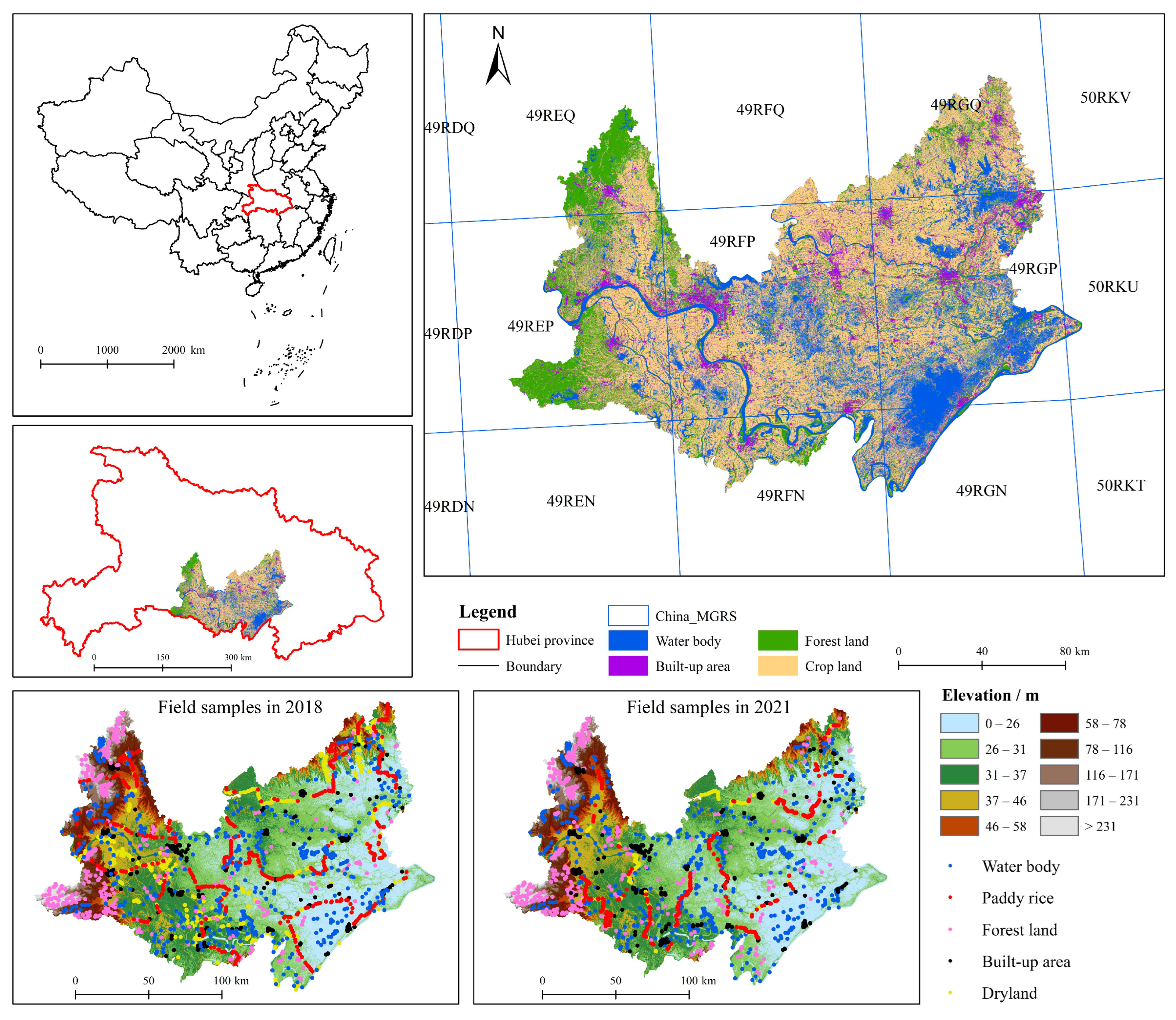
2.1. Study Area

The Jianghan Plain (JP) is a typical alluvial plain formed by the Yangtze River and its longest tributary, the Han River, located in the middle reach of the Yangtze River. It is located between latitudes ${29}^{\circ }{26}^{\prime }$ and ${31}^{\circ }{37}^{\prime }$N and longitudes ${111}^{\circ }{14}^{\prime }$ and ${114}^{\circ }{36}^{\prime }$E. It covers an area of approximately 30,000 km² and consists of 16 counties (or county-level municipalities or county-level districts) in the Hubei province. The subtropical monsoon climate of the JP offers an annual precipitation of about 1100 mm and a mean annual temperature of ~ 16.1 °C in four seasons [6]. The region is dominated by water bodies, built-up areas, and cropland with both dryland and paddy fields (Figure 1). Generally, rich water resources and abundant rainfall not only result in a plain that is ideal for paddy rice cropping but also render rice mapping from optical remote sensing imagery susceptible to cloud contamination.

2.2. Data

2.2.1. Remotely Sensed Data

The European Space Agency openly and freely provides Sentinel-2 data with a spatial resolution of 10 to 60 m depending on the spectral band. Hereby, all available Sentinel-2 Multi-Spectral Instrument (MSI) Level-1C (L1C) scenes covering the JP during the growing season in 2018 were used because this year is the first full calendar year that imagery from the constellation could be simultaneously used, and Sentinel-2 L1C top-of-atmosphere (TOA) imagery has been widely utilized in cropland mapping [9,11,33]. Furthermore, we collected Level-2A (L2A) surface reflectance (SR) in 2021 to compare the performance of rice mapping with L1C datasets in different machine-learning algorithms. The onboard MSI sensor with visible, near-infrared (NIR), and shortwave infrared (SWIR) bands contains 13 channels: four bands at 10 m (visible and NIR), six bands at 20 m (vegetation red edge, narrow NIR, and SWIR) and three bands at 60 m (coastal aerosol, water vapor, and SWIR-cirrus). In our research, eleven Sentinel-2 bands which ranged from visual to SWIR, and remote sensing spectral indices were calculated (

Table 1. Description of remote sensing data used in this study.

Bands	Central Wavelength	Space Resolution	Purpose (Cloud-Mask Algorithm/VI)
Blue (B2)	492.4 nm (S2A)/492.1 nm (S2B)	10 m	CloudScore/BSI, EVI, PSRI
Green (B3)	559.8 nm (S2A)/559.0 nm (S2B)	10 m	CloudScore/GCVI, MNDWI
Red (B4)	664.6 nm (S2A)/664.9 nm (S2B)	10 m	CloudScore/BSI, NDVI, EVI, PSRI, MTCI
RE 1 (B5)	704.1 nm (S2A)/703.8 nm (S2B)	20 m	-/MTCI
RE 2 (B6)	740.5 nm (S2A)/739.1 nm (S2B)	20 m	-/PSRI, MTCI
RE 3 (B7)	782.8 nm (S2A)/779.7 nm (S2B)	20 m	CDI
NIR (B8)	832.8 nm (S2A)/833.0 nm (S2B)	10 m	CloudScore, CDI/BSI, NDVI, EVI, GCVI, LSWI, NDBI
NIR (B8A)	864.7 nm (S2A)/864.0 nm (S2B)	20 m	CDI
Cirrus (B10)	1373.5 nm (S2A)/1376.9 nm (S2B)	60 m	QA60
SWIR1 (B11)	1613.7 nm (S2A)/1610.4 nm (S2B)	20 m	CloudScore/BSI, MNDWI, NDBI
SWIR2 (B12)	2202.4 nm (S2A)/2185.7 nm (S2B)	20 m	CloudScore/LSWI

).

2.2.2. Field Survey Data

Field survey data served as the ground truth data for classifier training and validation of classification results. The ground truth data of JP was collected from two field surveys of land cover in the summer of 2018 and 2021. Specifically, using GVG (GPS-Video-GIS) software [34], an application that can gather GPS (Global Positioning System) information from camera photos based on a smartphone, we recorded the land cover types of field samples and their geographic positions. Due to road conditions, some field samples were located at the ridge of the field or on the roadsides next to paddy fields. Consequently, we examined these samples using high-resolution Google Earth data and 0.75 m resolution Jilin-1 satellite imagery to rectify the land-cover type information of the samples. In the end, we collected a total of 2266 and 2296 field samples in five different land-cover categories (paddy fields, dry land, water bodies, forest land, and building area) in 2018 and 2021, respectively. These samples were separated into two parts: about 70% of the samples were used for training machine-learning classifiers, and the remaining 30% were used for validation (see

Table 2. The number of ground truth samples in 2018 and 2021.

Class	Training		Validation		Total
	2018	2021	2018	2021	2018	2021
Water body	329	330	141	142	470	472
Built-up area	255	252	109	108	364	360
Forest land	265	258	113	110	378	368
Dryland	328	232	140	100	468	332
Paddy rice	410	535	176	229	586	764
Total	1587	1607	680	689	2266	2296

for details).

2.2.3. Other Reference Data

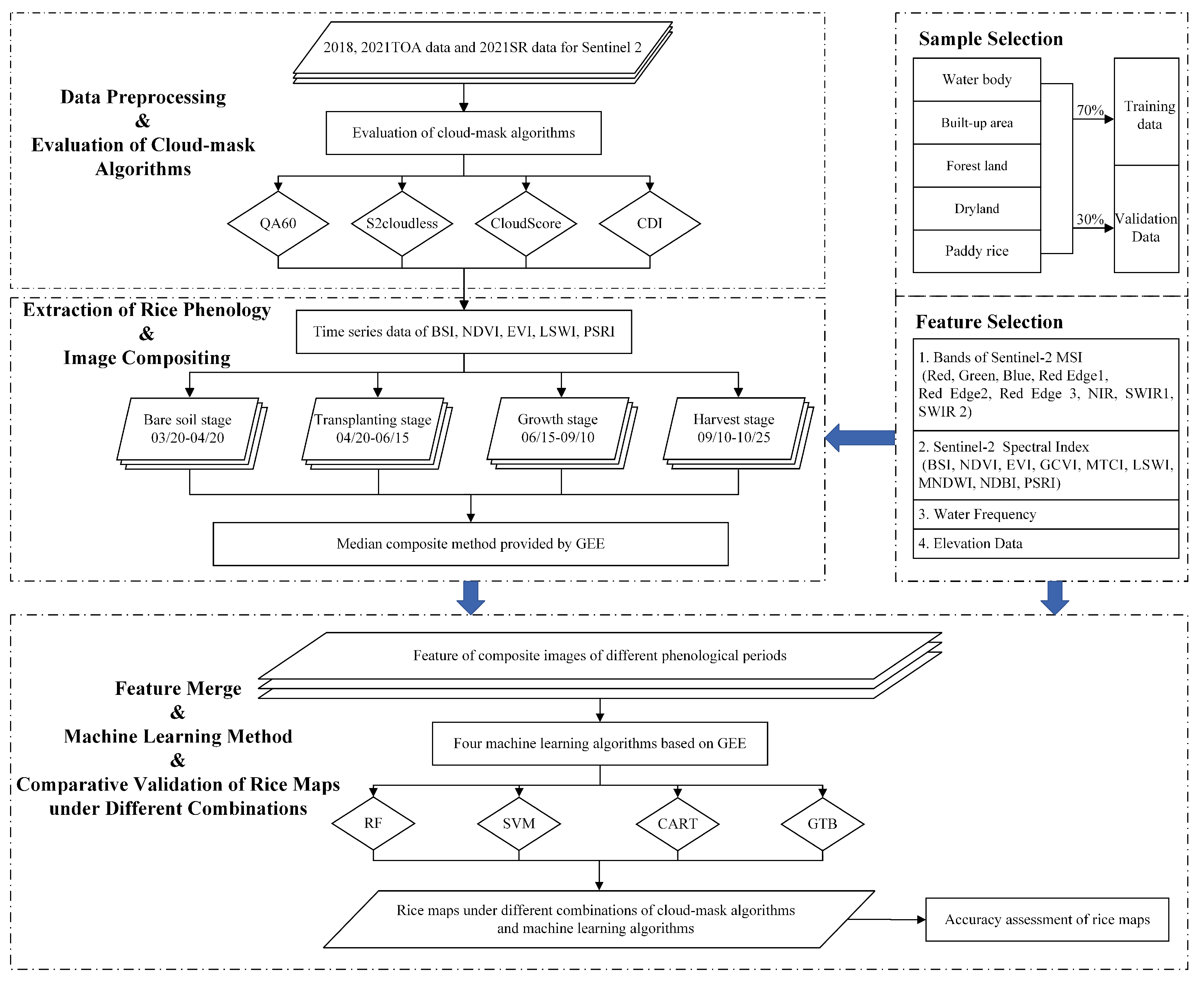
In addition to field survey data, a recently published Chinese rice map collection was used to evaluate the spatial distribution similarity of the generated rice maps. The map collection contains a series of single-cropping rice maps from 2017 to 2022 with a resolution of 10 m. These rice maps were generated from Sentinel-1A and Sentinel-2 data by comparing the dissimilarity of each pixel with the standard rice pixel in the time series. The accuracy assessment was examined using more than 100,000 field samples as well as county-level statistical data, and the average overall accuracy was greater than 85% [35]. The JP region of the rice maps for 2018 and 2021 was clipped for comparison.

In addition, the rice paddy area derived from the Hubei rural statistical yearbook of 2018 and 2021 was used for validation. The statistical data was compiled at the county level, and the data from 16 counties in the JP was collected for comparison.

3. Methodology

The overall process of this study included three stages, as shown in Figure 2. In the beginning, we used cloud-mask algorithms for cloud removal in the TOA and SR datasets of Sentinel-2 and evaluated the algorithms for each cloud-masked dataset. Next, the median composite method was used to generate cloud-free composite images based on the phenology stages of paddy rice in the JP. Lastly, we used selected features of composite images to map paddy rice with machine-learning classifiers and compared different combinations of cloud-mask algorithms and classifiers in rice mapping.

3.1. Cloud-Mask Algorithms

(1)

QA60

The Sentinel user guides online offer a detailed description of QA60 (https://sentinel.esa.int/web/sentinel/technical-guides/sentinel-2-msi/level-1c/cloud-masks, accessed on 21 December 2023). In brief, dense clouds were identified by B2, B11, and B12 using the threshold method, and cirrus clouds were detected by B10 based on spectral criteria. The quality layer of QA60 was embedded in Sentinel-2 data and flagged the opaque cloud pixels (Bit 10) and cirrus cloud pixels (Bit 11) [36]. Cloud-contaminated pixels flagged as 1 by Bit 10 or Bit 11 in the QA60 band were masked in GEE.

(2)

Sentinel-2 cloud detector (S2cloudless)

Using the Light Gradient Boost Machine (Light GBM) framework, one kind of tree-based learning algorithm, Sentinel-2 cloud detector (S2cloudless), provides automated cloud detection in Sentinel-2 imagery. Sentinel Hub’s research team led the development of the classifier based on a single-scene pixel-based cloud detector. The detailed description can be found in [26,30] (https://medium.com/sentinel-hub/cloud-masks-at-your-service-6e5b2cb2ce8a, accessed on 15 December 2023). Fortunately, at present, the S2 cloudless mask is available as a precomputed layer within Sentinel Hub and has been used to produce a Sentinel-2 cloud probability dataset for developers that is easy to use (https://developers.google.com/earth-engine/datasets/catalog/COPERNICUS_S2_CLOUD_PROBABILITY, accessed on 15 December 2023). Ref. [26] recommended a threshold value of 0.4 to minimize cloud omission errors in this algorithm.

(3)

CloudScore algorithm

The CloudScore algorithm is a pixel-wise cloud and cloud shadow masking method initially used with Landsat imagery [31]. It used visible, NIR, SWIR, and thermal bands to identify and remove clouds by scoring pixels by their relative cloudiness. The algorithm has been embedded in GEE as an internal function (‘ee.Algorithms.Landsat.simpleCloudScore’) and was successfully improved for cloud detection in Sentinel-2 MSI data using cirrus and aerosol bands to substitute the thermal infrared (TIR) band of Landsat [32]. The definition of the cloud score and its processing with the GEE platform was described in [32].

(4)

Cloud Displacement Index (CDI)

The CDI algorithm utilizes the parallax of the near-infrared (NIR) bands between the TOA dataset and SR dataset of Sentinel-2 imagery to enhance cloud detection. Reliable separation of clouds from the surface in Sentinel-2 data is achieved by calculating the parallax between the near-infrared bands for the observation angle. This is used to fully compensate for the missing thermal infrared bands and is primarily targeted at the detection of low-level clouds and surface objects within the coverage of low-level clouds [27]. Since the GEE platform did not offer the SR dataset of the JP in 2018 and the CDI algorithm requires both the TOA dataset and the SR dataset, we will only use the CDI algorithm for cloud removal in 2021.

3.2. Paddy Rice Mapping Algorithms

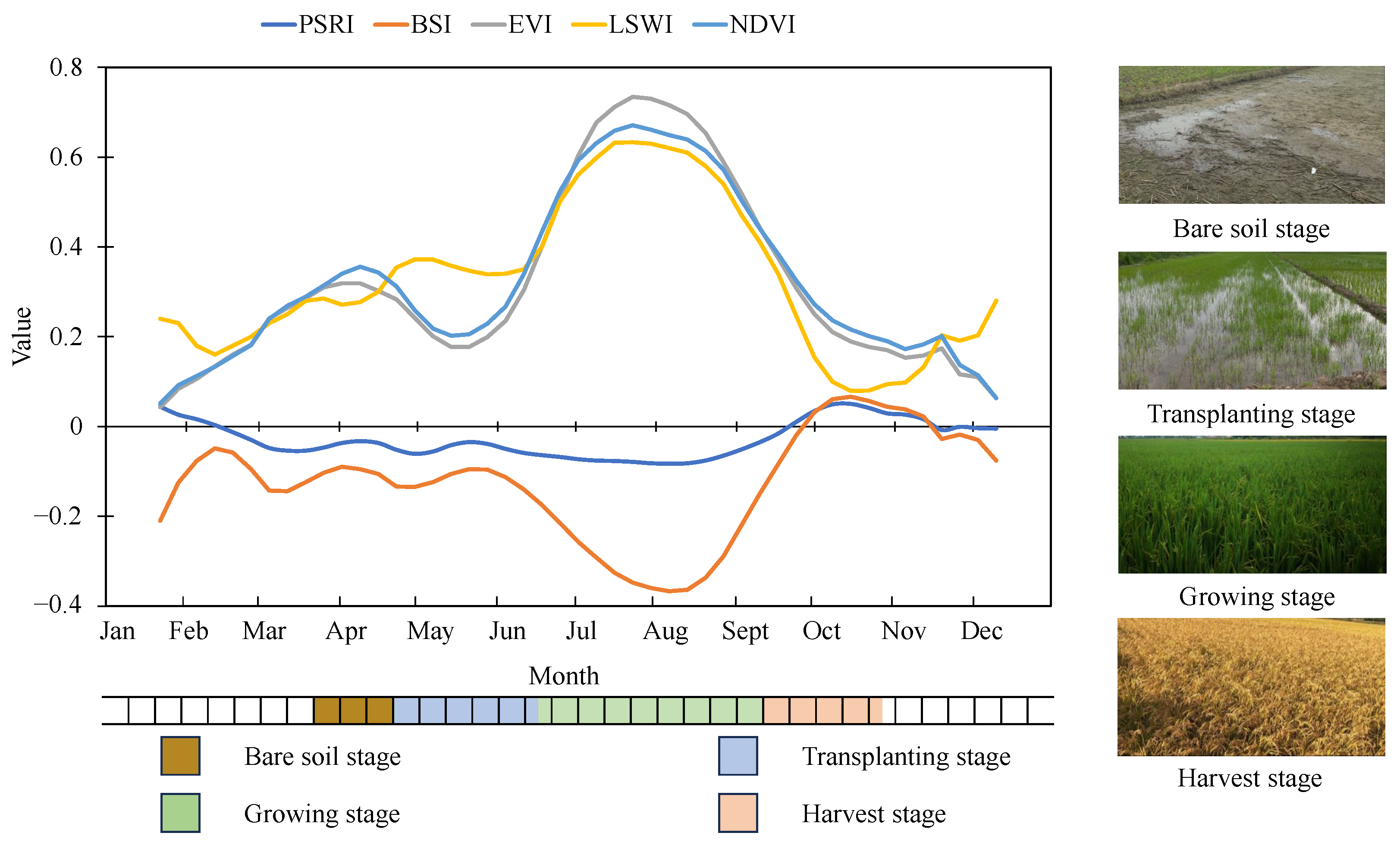
3.2.1. Extraction Phenology of Paddy Rice

In the JP, single-cropping rice is dominated in paddy fields [37], and its growing season ranged from late March to late October, according to our field surveys in 2018 and 2021 as well as relevant research on rice mapping in the Hubei province [9,38]. Based on the cloud-masked imagery, we generated time-series datasets of five spectral indices (BSI, LSWI, NDVI, EVI, and PSRI) using 200 rice samples in 2018 and 2021, respectively. These datasets were smoothed by the Savitzky-Golay (SG) filter with a smoothing window of 30 and a degree of the smoothing polynomial of 5 based on repeated testing (Figure 3). We examined and compared smoothed time-series curves produced by the TOA datasets and SR datasets and discovered a lot of similarities between them. Four featured phenology stages were detected from time-serious observations of the five spectral indices by their day of year (DOY). These key stages were: (1) the bare soil stage, which is a period before transplanting. During this stage, NDVI and EVI gradually rose with the growth of the weed and then started to decrease when the soil was turned before planting. Meanwhile, BSI obtains relatively high values compared with theirs in the growing stage [11]; (2) transplanting stage: paddy fields were flooded and then transplanted during this period. LSWI increased rapidly, and its value greater than NDVI and EVI was recognized as the flooding and transplanting signal [7]; (3) growing stage: both NDVI and EVI grow dramatically faster than LSWI in the early growing period, implying paddy rice gradually dominated paddy fields due to the degradation of water signal. Then, the three indices reached their peaks while BSI descended the trough at the same stage; (4) harvest stage, the stage in which NDVI and EVI decreased sharply owing to the reduction of greenness and chlorophyll of paddy rice, while BSI and PSRI showed a rapid rise due to the enhancement of soil signal and substantial changes in carotenoid and chlorophyll content (

Table 3. Time windows for phenological stages of single-cropping rice in the JP.

Phenology Stages	Time Windows
Bare soil stage	20/03–20/04
Transplanting stage	20/04–15/06
Growing stage	15/06–10/09
Harvest stage	10/09–25/10

).

According to the spectral characteristics of paddy fields analyzed above and the latest associated research, we selected three types of features for rice mapping. The first type was bands of Sentinel-2 MSI, including Blue, Green, Red, Red Edge1, Red Edge2, Red Edge3, NIR, SWIR1, and SWIR2. The performance of red-edge bands has been widely explored in vegetation monitoring, and highly evaluated in rice mapping in recent studies [11]. Second, we used one soil index (BSI)), four vegetation indices (NDVI, EVI, GCVI, and PSRI), one red-edge index (MTCI), two water indices (MNDWI and LSWI), and one building index (NDBI) (

Table 4. Spectral indices and their expressions used in this study.

Spectral Indices	Expressions	References
Bare Soil Index (BSI)	$\mathrm{BSI}=\frac{\left(\mathrm{SWIR}1+\mathrm{Red}\right)-\left(\mathrm{NIR}+\mathrm{Blue}\right)}{\left(\mathrm{SWIR}1+\mathrm{Red}\right)+\left(\mathrm{NIR}+\mathrm{Blue}\right)}$	[40]
Normalized Difference Vegetation Index (NDVI)	$\mathrm{NDVI}=\frac{\mathrm{NIR}-\mathrm{Red}}{\mathrm{NIR}+\mathrm{Red}}$	[41]
Enhanced Vegetation Index (EVI)	$\mathrm{EVI}=\frac{2.5\times \left(\mathrm{NIR}-\mathrm{Red}\right)}{\mathrm{NIR}+6\times \mathrm{Red}-7.5\times \mathrm{Blue}+1}$	[42]
Green Chlorophyll Vegetation Index (GCVI)	$\mathrm{GCVI}=\frac{\mathrm{NIR}}{\mathrm{Green}}-1$	[15]
Plant Senescence Reflectance Index (PSRI)	$\mathrm{PSRI}=\frac{\mathrm{Red}-\mathrm{Blue}}{\mathrm{Red}\mathrm{Edge}2}$	[43]
MERIS Terrestrial Chlorophyll Index (MTCI)	$\mathrm{MTCI}=\frac{\mathrm{Red}\mathrm{Edge}2-\mathrm{Red}\mathrm{Edge}1}{\mathrm{Red}\mathrm{Edge}2+\mathrm{Red}}$	[44]
Modified Normalized Difference Water Index (MNDWI)	$\mathrm{MNDWI}=\frac{\mathrm{Green}-\mathrm{SWIR}1}{\mathrm{Green}+\mathrm{SWIR}1}$	[45]
Land Surface Water Index (LSWI)	$\mathrm{LSWI}=\frac{\mathrm{NIR}-\mathrm{SWIR}2}{\mathrm{NIR}+\mathrm{SWIR}2}$	[12]
Normalized Difference Built-Up Index (NDBI)	$\mathrm{NDBI}=\frac{\mathrm{NIR}-\mathrm{SWIR}1}{\mathrm{NIR}+\mathrm{SWIR}1}$	[46]

). The advantages of these indices in rice mapping were greatly valued in a few studies [8,39]. Moreover, year-round synthetic images were used to calculate the water frequency and served as a feature to distinguish rice paddies from water bodies. The last type was DEM, which proved to be useful for rice mapping in plain areas [15] because water storage is easy in flat areas. In each phenological stage, images were composited by using the median values of all cloud-masked bands and spectral index imagery.

3.2.2. Machine-Learning Algorithms

Machine-learning algorithms have been widely used in rice mapping. Here, we examined the mapping performance of four regular algorithms that were embedded in GEE. Normally, 70% of the samples were used for training, and the remaining 30% were selected as the validation data.

(1) Random Forest (RF). RF is a decision tree-based classifier that integrates multiple decision trees through the idea of integrated learning. It combines individual decision trees using a series of subsets of training samples, and these multiple decision trees with high variance and low bias form several user-defined trees, which can be integrated to vote for category membership [47]. In GEE, we used the function ‘ee.Classifier.smileRandomForest’ to create an RF classifier. The parameters of the algorithm, such as the number of trees, bag fraction, and so on, were optimized through the testing of different combinations. Lastly, 410 and 0.8 were confirmed as the final combination regarding higher accuracy and relatively high efficiency.

(2) Support Vector Machine (SVM). SVM is a supervised machine-learning algorithm and the basic principle of the algorithm is to construct a maximum margin hyperplane for distinguishing different feature types in high-dimensional feature space based on training data [48]. In GEE, we built an SVM classifier by using the function of ‘ee.Classifier.libsvm()’, and selected the radial basis function (RBF) as the kernel function type for classification because of its simplicity, time efficiency, and ability to produce accurate results [49,50]. When using RBF as the kernel type, two hyperparameters (‘gamma’ and ‘c’, used to give curvature weight of the decision boundary and control error, respectively) need to be set before the training model. For choosing gamma, we tested values like 0.001, 0.01, 0.1, 1, 10, and 100, while the same tested for ‘c’ values. Through the parameter tuning experiment, we chose the optimal combination of 0.01 for ‘gamma’ and 10 for ‘c’.

(3) Classification and Regression Tree (CART). The algorithm creates a tree-like structure that divides the dataset into different subsets, each of which corresponds to a leaf node of the tree. In short, it is a tree of multiple decision rules, and all these rules will be derived from the data features. In our study, the ‘ee.Classifier.cart()’ function was used to create the CART classifier in the GEE platform. The main parameters within the classifier include ‘minLeafPopulation’ and ‘maxNodes’, whose optimal values were 1 and 10 after different tests, respectively.

(4) Gradient Tree Boost (GTB). It is an integrated learning method that builds a strong learner by combining multiple weak learners (e.g., shallow trees) and is suitable for dealing with complex, high-dimensional datasets and non-linear relationships. In GEE, we used the ‘ee.Classifier.smileGradientTreeBoost()’ function to conduct the classifier. Among many parameters, two critical hyperparameters, ‘number of trees’ and ‘shrinkage’ (also known as the ‘learning rate’), strongly influenced the efficiency and robustness of the algorithm. Other parameters included ‘sampling rate’, ‘max nodes’, and ‘seed’. We set the values of the above parameters in order: 100, 0.005, 0.7, 50, and 10 through the testing of different combinations.

3.3. Assessment of Cloud-Mask Algorithms and Rice Maps

3.3.1. Assessment of Cloud-Mask Algorithms

To provide a comprehensive evaluation of the four cloud mask algorithms, we selected three Sentinel-2 granules to conduct the assessment. These granules are also called tiles, which are the minimum indivisible partitions in the MSI sensor reference frame of a given number of lines along the track and detector-separated. The tile IDs are 49REP, 49RFP, and 49RGP, which extensively covered the JP area from west to east. Due to the uneven duration of each paddy rice growing stage, we chose two tiles acquired in the growing stage and one tile within the bare soil stage, transplanting stage, and harvest stage, respectively, resulting in a total of five time-series images for each granule (

Table 5. The summary of samples used for the evaluation of cloud-mask algorithms.

Data Type	Tile	Phenology Stages	Date	Cloud Cover/%	Samples
					Cloud	Clear	Total
2018TOA	49REP	Bare soil stage	3/4/2018	7.4915	161	240	401
		Transplanting stage	23/5/2018	33.6128	235	182	417
		Growing stage	27/6/2018	15.294	187	261	448
			6/8/2018	23.0023	304	120	424
		Harvest stage	10/10/2018	5.3781	84	389	473
	49RFP	Bare soil stage	8/4/2018	16.5152	217	252	469
		Transplanting stage	28/4/2018	15.0278	260	225	485
		Growing stage	17/7/2018	45.5232	212	201	413
			1/8/2018	14.4641	251	178	429
		Harvest stage	15/9/2018	8.6775	253	259	512
	49RGP	Bare soil stage	8/4/2018	15.6042	114	253	367
		Transplanting stage	8/5/2018	41.6684	281	133	414
		Growing stage	17/6/2018	49.8558	259	146	405
			22/7/2018	1.9465	204	237	441
		Harvest stage	10/10/2018	0.898	77	328	405
2021TOA	49REP	Bare soil stage	12/4/2021	8.066	262	205	467
		Transplanting stage	11/6/2021	63.7011	352	108	460
		Growing stage	5/8/2021	33.6629	220	191	411
			9/9/2021	55.6306	267	155	422
		Harvest stage	24/10/2021	10.93	179	247	426
	49RFP	Bare soil stage	28/3/2021	47.4834	279	129	408
		Transplanting stage	1/6/2021	34.2679	273	156	429
		Growing stage	21/7/2021	26.6127	242	129	371
			4/9/2021	34.5427	190	198	388
		Harvest stage	24/10/2021	8.3527	263	160	423
	49RGP	Bare soil stage	12/4/2021	33.8914	265	150	415
		Transplanting stage	17/5/2021	17.7569	227	202	429
		Growing stage	5/8/2021	19.443	261	152	413
			20/8/2021	32.4015	254	161	415
		Harvest stage	29/9/2021	18.0409	198	212	410
2021SR	49REP	Bare soil stage	12/4/2021	12.200443	262	205	467
		Transplanting stage	11/6/2021	75.641401	352	108	460
		Growing stage	5/8/2021	35.574219	220	191	411
			9/9/2021	47.876539	267	155	422
		Harvest stage	24/10/2021	7.954566	179	247	426
	49RFP	Bare soil stage	28/3/2021	61.947279	279	129	408
		Transplanting stage	1/6/2021	46.110165	273	156	429
		Growing stage	21/7/2021	17.516239	242	129	371
			4/9/2021	27.806534	190	198	388
		Harvest stage	24/10/2021	6.579728	263	160	423
	49RGP	Bare soil stage	12/4/2021	61.947279	265	150	415
		Transplanting stage	17/5/2021	42.097832	227	202	429
		Growing stage	5/8/2021	22.158073	261	152	413
			20/8/2021	23.202318	254	161	415
		Harvest stage	29/9/2021	9.179795	198	212	410

). The cloud cover of these tiles ranged from 0 to 80%, assigning to different growing stages of paddy rice. As each Sentinel-2 tile covers a surface area of 110 km × 110 km with a 10 m spatial resolution, previous studies on cloud-mask algorithm evaluation have shown that using about 400 validation samples per image can achieve a 95% confidence level with a 5% margin of error. Therefore, we labeled approximately 400 samples with labels of ‘cloud’ and ‘non-cloud’ (clear) for each tile given dense, cirrus, and haze cloud types in ‘cloud’ labels and different land cover types (e.g., water bodies, cropland, buildings, and forest) in ‘non-cloud’ labels. The detailed information on selected images and sample labeling is listed in Table 5. Based on the sample labeling, we used the confusion matrix to generate producer accuracy (PA), user accuracy (UA), and overall accuracy (OA) for the assessment of the four cloud-mask algorithms. Finally, five evaluation metrics for one year were averaged to assess the performances of the four cloud-mask algorithms in the TOA dataset of 2018, and the same tiles were used for the evaluations of the TOA and SR datasets in 2021.

3.3.2. Feature Evaluation of Different Cloud-Free Datasets

In addition to the assessment of cloud-mask algorithms, the quality of the cloud removal imagery that would be input into the machine-learning model also needs to be investigated. We calculated the spectral separability of samples in the cloud-masked imagery. Based on the different spectral responses of vegetation and non-vegetation, the Jeffries-Matusita (J-M) distance has been proven to be an efficient measure for assessing spectral separability in vegetation mapping by remote sensing [51]. The spectral separability was determined by calculating the J-M values of various land cover samples in feature datasets. It calculates a measure of distance between two classes, and the formula is presented below:

$$J_{ij}=2\left(1-e^{-B_{ij}}\right)$$

(1)

$$B_{ij}=\frac{1}{8}{\left(m_i-m_j\right)}^2\frac{2}{v_i^2+v_j^2}+\frac{1}{2}\left[\frac{v_i^2+v_j^2}{2v_i{v}_j}\right]$$

(2)

where $J_{ij}$ is the separability measure of class i from class j, B is the Bhattacharyya distance, $m_i$, $m_j$ are the means, and $v_i$, $v_j$ are the variances of classes i and j [52]. J-M values range from 0 to 2. A larger J-M distance indicates a higher degree of separation between categories, which usually implies better classification performance [53].

3.3.3. Validation of Rice Maps

The evaluation of the rice maps was compared with the latest 10 m resolution rice map, and a spatial distribution similarity assessment proposed by Jaccard [54] was employed. This statistical metric is a way to assess two sets’ similarity, which is typically used to gauge how much overlap there is between them. This metric is especially suitable for the case where the elements of two sets are binary, which corresponds to the rice and non-rice categories in our study. The formula for Jaccard similarity is as follows:

$$J\left(A,B\right)=\left(|A\cap B|\right)/\left(|A\cup B|\right)$$

(3)

where $J(A,B)$ denotes the Jaccard similarity of sets A and B. $A\cap B$ denotes the number of elements in the intersection, i.e., the number of elements shared by the two sets. $A\cup B$ denotes the number of elements in the union set, i.e., the total number of all non-repeating elements in the two sets. The value of the Jaccard similarity metric ranges from 0 to 1. In this study, we used the reference rice maps as A and generated rice maps as B (in which all the rice attributes were 1 and the non-rice attributes were 0). We determined the spatial distribution similarity of the two rice maps by calculating the Jaccard similarity.

Finally, we compared the rice-cropped area derived from our study with that extracted from the statistical yearbook of the Hubei Province in 2018 and 2021. The metrics of the coefficient of determination (R²) and the root mean square error (RMSE) were used to evaluate the comparisons at the county level.

4. Results

4.1. Evaluations of Cloud-Mask Algorithms

4.1.1. Accuracy Assessment of the Four Cloud-Mask Algorithms

Table 6. Accuracy evaluation of four cloud-mask algorithms.

Data Type	Tile	Label	QA60		S2cloudless		CloudScore		CDI
			PA (%)	UA (%)	PA (%)	UA (%)	PA (%)	UA (%)	PA (%)	UA (%)
2018TOA	REP	Cloud	66.68	95.16	92.47	98.09	83.10	93.69	-	-
		Clear	98.19	75.90	97.28	96.48	95.46	92.13	-	-
		OA(%)	83.18		96.94		93.45		-
	RFP	Cloud	72.67	96.97	95.97	92.06	82.51	92.07	-	-
		Clear	97.48	78.05	87.27	95.82	90.39	85.82	-	-
		OA(%)	84.46		92.01		86.85		-
	RGP	Cloud	58.42	96.31	92.92	97.23	77.56	87.22	-	-
		Clear	95.40	72.62	95.70	96.55	89.84	89.48	-	-
		OA(%)	80.09		96.47		88.88		-
2021TOA	REP	Cloud	69.65	99.39	99.29	98.10	99.57	96.16	-	-
		Clear	99.26	68.96	97.07	99.13	95.67	99.41	-	-
		OA(%)	81.72		98.54		97.72		-
	RFP	Cloud	67.86	96.73	99.02	98.66	97.36	96.50	-	-
		Clear	97.21	69.78	97.50	98.38	93.76	96.36	-	-
		OA(%)	77.71		98.52		96.09		-
	RGP	Cloud	47.50	95.90	96.97	97.75	99.36	97.58	-	-
		Clear	97.22	58.22	95.78	96.54	96.54	99.04	-	-
		OA(%)	69.21		96.86		98.19		-
2021SR	REP	Cloud	69.88	99.39	99.51	98.11	98.26	98.93	98.31	81.06
		Clear	99.26	69.10	97.07	99.29	98.63	97.86	59.16	95.09
		OA(%)	81.82		98.64		98.49		83.70
	RFP	Cloud	67.95	96.73	99.09	98.66	93.68	98.89	99.28	87.75
		Clear	97.21	69.89	97.50	98.46	98.21	92.45	72.83	97.78
		OA(%)	77.85		98.64		95.47		89.92
	RGP	Cloud	47.54	95.92	96.98	97.75	99.12	97.95	92.40	79.49
		Clear	97.26	58.27	95.78	96.57	97.16	98.69	63.85	87.17
		OA(%)	69.36		96.92		98.28		81.68
Total		Cloud	63.13	96.94	96.91	97.38	92.28	95.33	96.63	82.77
		Clear	97.61	68.98	95.66	97.47	95.07	94.58	65.28	93.35
		OA(%)	78.38		97.06		94.82		85.10

shows PA, UA, and OA for each cloud-mask algorithm. As SR products were required in the CDI algorithm, the evaluation of the TOA products was conducted using the algorithms of QA60, S2cloudless, and CloudScore. For TOA products of 2018 and 2011, the S2cloudless algorithm has the highest OA of the three algorithms except for the RGP tile of 2021 TOA products, and CloudScore shows substantially larger OAs than that of QA60. For the cloudy pixels in TOA products of 2018, S2cloudless holds a larger PA than that of CloudScore and QA60, while QA60 has the lowest PA among the three algorithms. Furthermore, S2cloudless has the largest UA in the tiles of REP and RGP, and QA60 has the largest UA in RFP tiles. For the clear pixels in TOA products of 2018, S2cloudless has the highest UA and QA60 has the lowest UA. For 2021 TOA products, S2cloudless has the largest PA and UA for cloudy pixels in the RFP tiles and the highest UA for cloudy pixels in the tiles of REP and RGP, while QA60 holds the smallest PA for cloudy pixels in the three tiles. For the SR products of 2021, S2cloudless and CloudScore have essentially larger OA than those of the QA60 and CDI algorithms. QA60 has the lowest PA for cloudy pixels and the lowest UA for clear pixels, respectively. Moreover, CDI holds the smallest PA for clear pixels and the smallest UA for cloudy pixels.

When comparing TOA products of 2018 with those of 2021 in the three tiles, S2cloudless and CloudScore algorithms have larger OAs in 2021 than those in 2018, while the facts of QA60 are just the opposite. When comparing TOA products with SR products in 2021, the differences in OA between TOA and SR are microscopic for QA60, S2cloudless, and CloudScore in the three tiles. Because of the specific tile, S2cloudless shows more overwhelming OAs than other algorithms in the RFP tile. Generally, the OAs from high to low are S2cloudless > CloudScore > QA60 for TOA products and S2cloudless > CloudScore > CDI > QA60 for SR products.

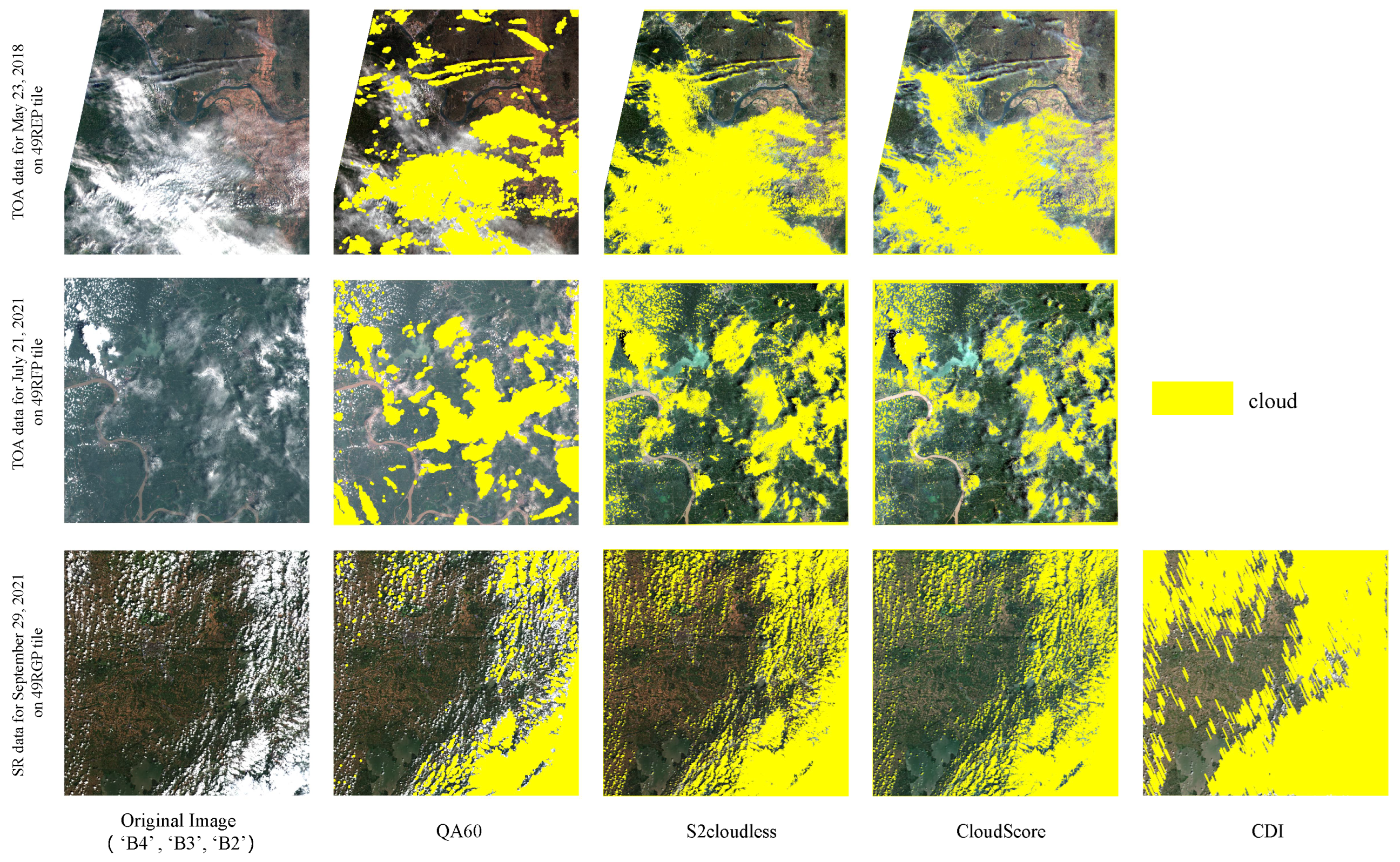
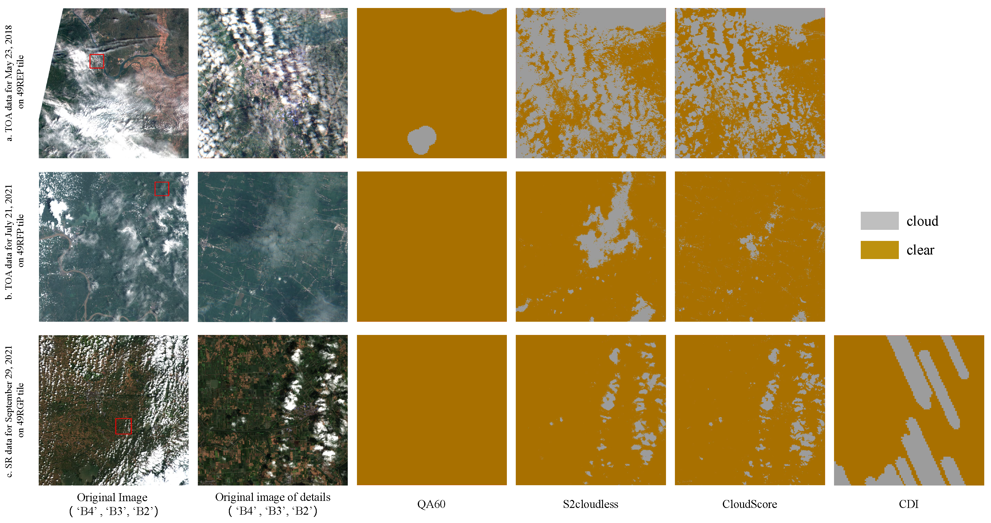
4.1.2. Visual Comparisons of the Four Cloud-Mask Algorithms

We also visually inspected the cloud removal of the three tiles (49REP, 49RFP, and 49RGP) (Figure 1) in different phenological stages of paddy rice. The results show that a few cloud pixels were mistakenly classified as clear pixels by QA60, and it performed poorly in identifying granular clouds and large-area clouds. In contrast, the S2cloudless algorithm excels at identifying cloud pixels, whether they are large-area clouds or granular clouds. CloudScore algorithms also perform well in the identification of cloud pixels. Nevertheless, banded features are displayed in the cloud pixel detection results of the CDI algorithm (Figure 4).

To further evaluate the detailed features after cloud removal, we selected three 10 × 10 km grids from the three tiles. As shown in Figure 5, a lot of pseudo-clear pixels are retained for the next procedure when masked by the QA60 algorithm. The S2cloudless algorithm shows overall excellent performance in identifying cloud pixels with detailed information. CloudScore algorithm exhibits a rather strong ability to remove cloud pixels, although it is slightly weak in haze removal (Figure 4 and Figure 5). For the CDI algorithm, the masks of cloud pixels appear in a stripe shape, and some clear pixels were removed while cloud pixels were retained.

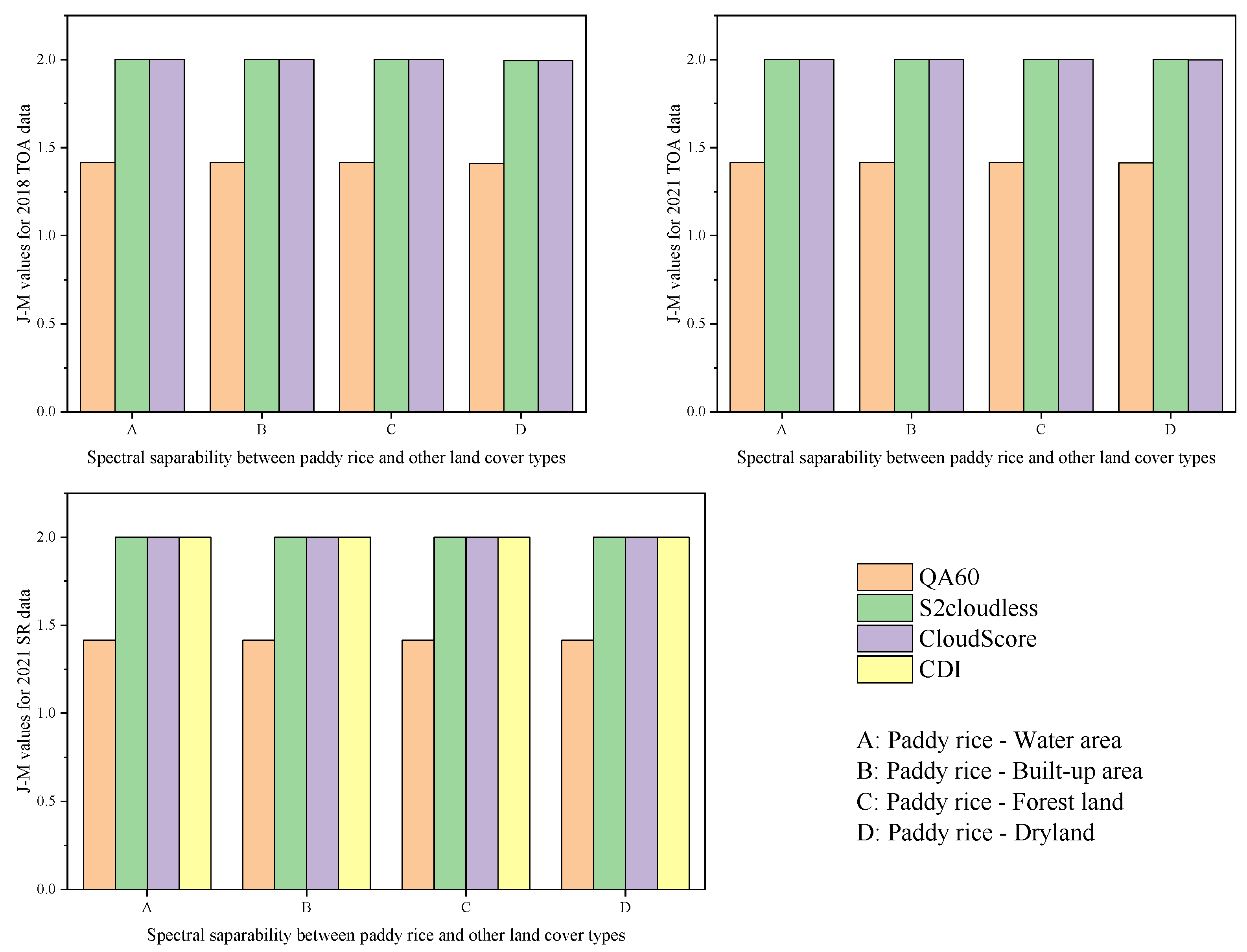
4.1.3. Spectral Separability between Paddy Rice and Other Land Cover Types in Cloud-Masked Imagery

Figure 6 shows the values of J-M distances of samples between paddy rice and other land cover types (water area, built-up area, forest land, and dryland) in the cloud-free imagery by different cloud-mask algorithms. The J-M values were about 1.4 when the imagery was masked by QA60. For the other three cloud-mask algorithms, all of the J-M values were greater than 1.9 between paddy rice and other land cover, implying high spectral separability in this cloud-masked imagery. The J-M values show minor gaps across TOA products and SR products.

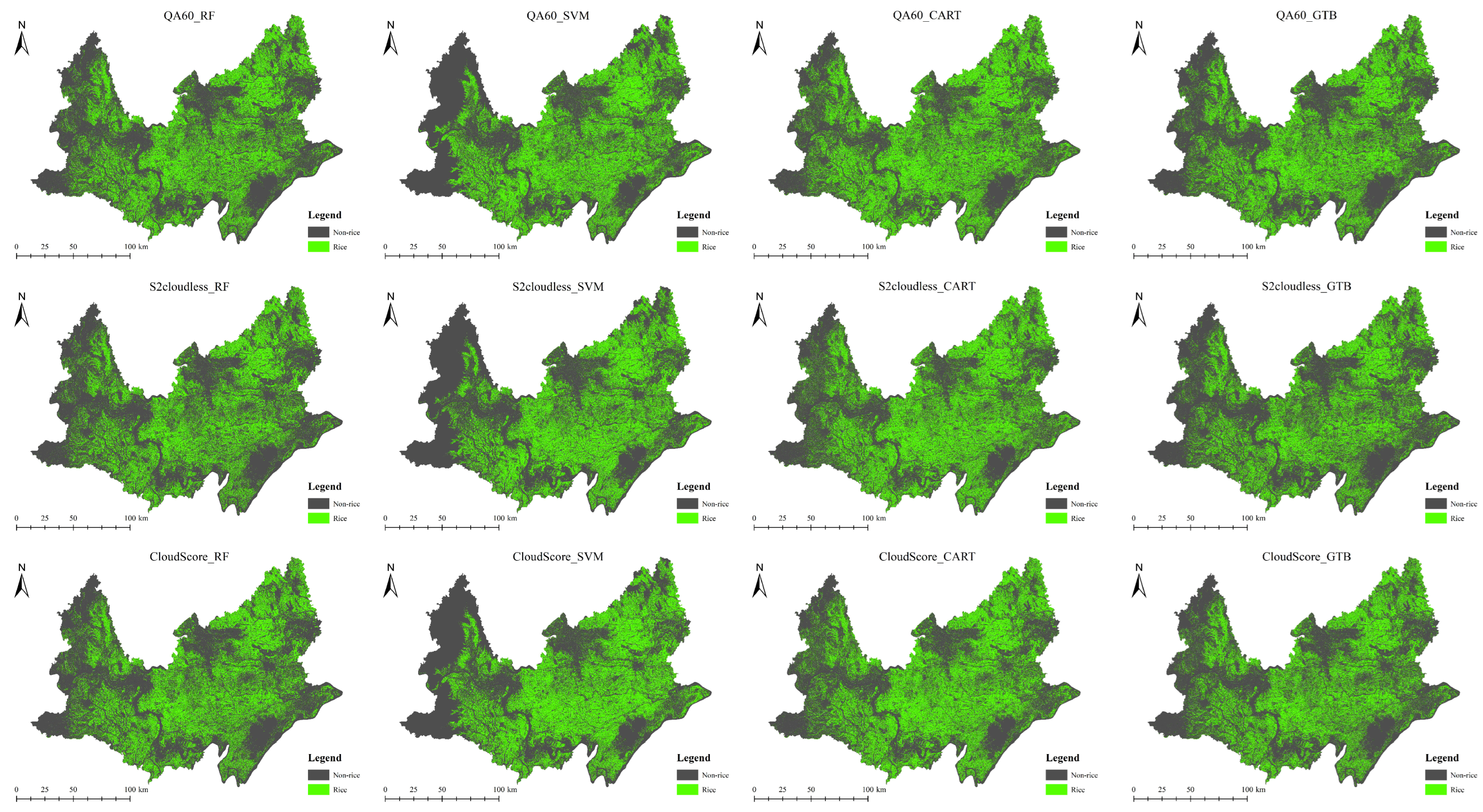
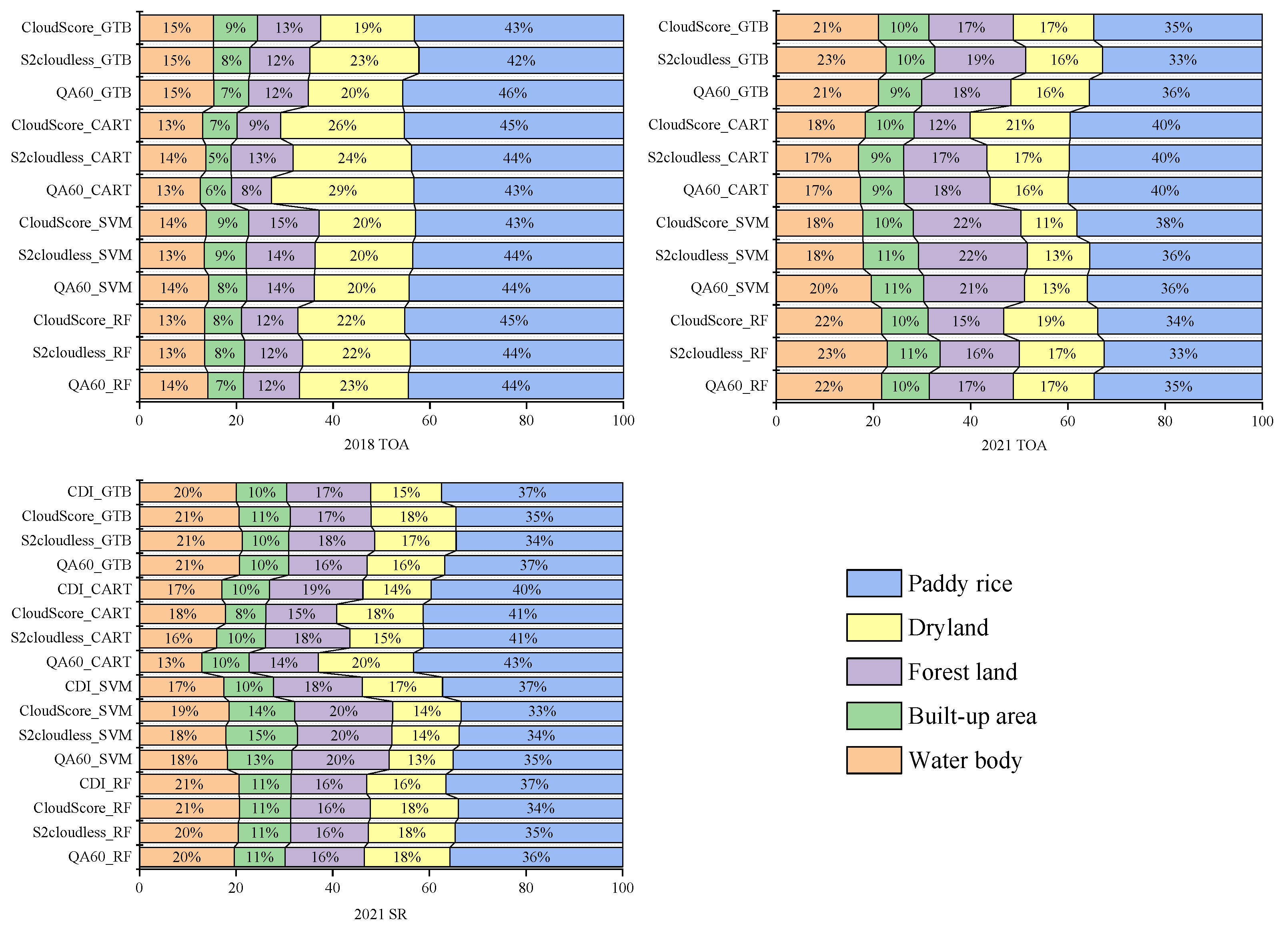
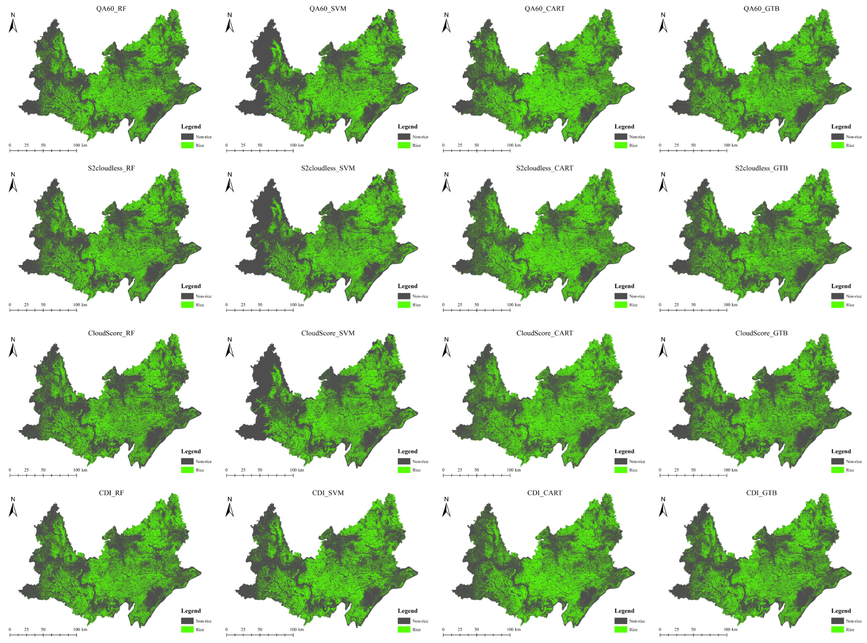
4.2. Rice Maps Extracted from the Algorithms of RF, SVM, CART and GTB

The integration of four machine-learning algorithms and four cloud-mask algorithms was used to map paddy rice in 2018 and 2021. As shown in Figure 7, rice cropped area (RCA) accounted for more than 40% and 30% of the JP area in 2018 and 2021, respectively. Specifically, RCA ranges from 12,028.1 to 12,990.4 km², varying with different machine-learning algorithms in 2018 (the spatial distribution maps of rice are shown in Appendix A). The result shows that the largest proportion of the JP area was covered by paddy fields; dry land came in second; the rest were in order of water bodies, forests, and built-up areas, except for the mapped result using the combination of SVM and S2cloudless as well as CloudScore algorithms. In 2021, RCA dropped from more than 40% to ~35% when using the methods of RF, SVM, and GTB, and fell to ~40% for the CART algorithm. Compared with RCA of 2018, the discrepancies of RCA extracted by the four machine-learning algorithms are greater in 2021, ranging from 9264.23 to 11,377.3 km² in TOA products and 9505.67 to 12,320.3 km² in SR products. Regarding RCA from TOA products and SR products in 2021, RCA from SR products is usually larger than that from TOA when using RF, CART, and GTB algorithms (except for the combination of GTB and CloudScore), while the result is contrary for the SVM algorithm. Additionally, there are some differences in the area of non-paddy fields between TOA products and SR products.

In summary, RCA showed a slight decline from approximately 45% of the entire JP area in 2018 to a range of approximately 33–40% in 2021, and dryland also showed a minor decrease during this period. The areas of water bodies, building area, and forest have indicated a mild rise from ~14 to ~20%, ~8 to ~10%, as well as ~12 to ~18% during 2018–2021, respectively.

4.3. Accuracy Assessment of Rice Maps

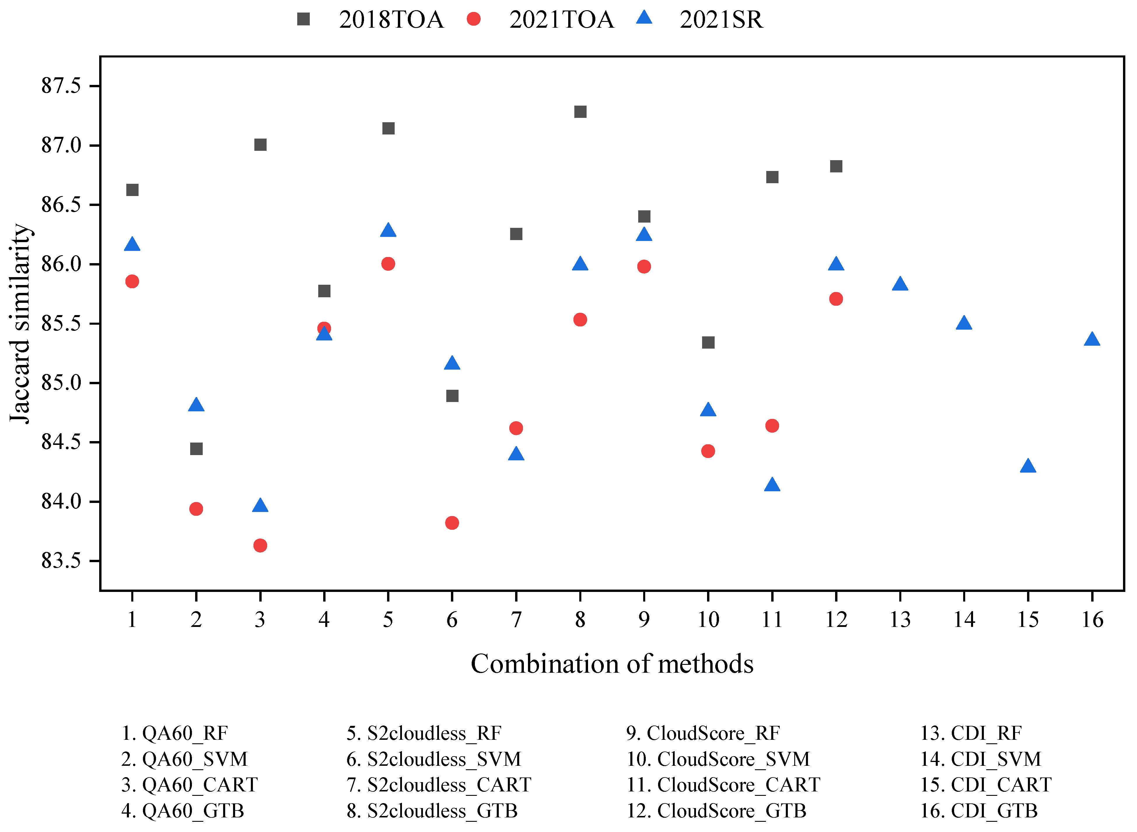
4.3.1. Comparing with Field Survey Data

As shown in

Table 7. Accuracy assessment of rice mapping with algorithm combinations.

Algorithm Combination	2018 TOA							2021 TOA							2021 SR
	Class	Rice	Non-Rice	PA (%)	UA (%)	OA (%)	Kappa	Class	Rice	Non-Rice	PA (%)	UA (%)	OA (%)	Kappa	Class	Rice	Non-Rice	PA (%)	UA (%)	OA (%)	Kappa
QA60-RF	Rice	149	27	84.66	78.84	90.15	0.75	Rice	171	5	97.16	95.53	98.09	0.95	Rice	173	3	98.3	94.02	97.94	0.95
	Non-rice	40	464	92.06	94.5			Non-rice	8	496	98.41	99			Non-rice	11	493	97.82	99.4
S2cloudless-RF	Rice	152	24	86.36	83.52	92.06	0.8	Rice	173	3	98.3	95.58	98.38	0.96	Rice	171	5	97.16	97.16	98.53	0.96
	Non-rice	30	474	94.05	95.18			Non-rice	8	496	98.41	99.4			Non-rice	5	499	99.01	99.01
CloudScore-RF	Rice	143	33	81.25	83.14	90.88	0.76	Rice	172	4	97.73	95.03	98.09	0.95	Rice	173	3	98.3	98.3	99.12	0.98
	Non-rice	29	475	94.25	93.5			Non-rice	9	495	98.21	99.2			Non-rice	3	501	99.4	99.4
CDI-RF	Rice							Rice							Rice	172	4	97.73	94.51	97.94	0.95
	Non-rice							Non-rice							Non-rice	10	494	98.02	99.2
QA60-SVM	Rice	146	30	82.95	75.26	88.53	0.71	Rice	164	12	93.18	92.13	96.18	0.9	Rice	170	6	96.59	94.44	97.65	0.94
	Non-rice	48	456	90.48	93.83			Non-rice	14	490	97.22	97.61			Non-rice	10	494	98.02	98.8
S2cloudless-SVM	Rice	151	25	85.8	78.24	90.15	0.75	Rice	170	6	96.59	93.41	97.35	0.93	Rice	168	8	95.45	94.38	97.35	0.93
	Non-rice	42	462	91.67	94.87			Non-rice	12	492	97.62	98.8			Non-rice	10	494	98.02	98.41
CloudScore-SVM	Rice	141	35	80.11	71.57	86.62	0.66	Rice	168	8	95.45	91.3	96.47	0.91	Rice	167	9	94.89	94.35	97.21	0.93
	Non-rice	56	448	88.89	92.75			Non-rice	16	488	96.83	98.39			Non-rice	10	494	98.02	98.21
CDI-SVM	Rice							Rice							Rice	168	8	95.45	93.33	97.06	0.92
	Non-rice							Non-rice							Non-rice	12	492	97.62	98.4
QA60-CART	Rice	146	30	82.95	75.26	88.53	0.71	Rice	170	6	96.59	91.4	96.76	0.92	Rice	166	10	94.32	88.3	95.29	0.88
	Non-rice	48	456	90.48	93.83			Non-rice	16	488	96.83	98.79			Non-rice	22	482	95.63	97.97
S2cloudless-CART	Rice	147	29	83.52	79.46	90.15	0.75	Rice	170	6	96.59	91.89	96.91	0.92	Rice	172	4	97.73	90.05	96.62	0.91
	Non-rice	38	466	92.46	94.14			Non-rice	15	489	97.02	98.79			Non-rice	19	485	96.23	99.18
CloudScore-CART	Rice	138	38	78.41	73.02	86.91	0.67	Rice	174	2	98.86	88.32	96.32	0.91	Rice	171	5	97.16	95	97.94	0.95
	Non-rice	51	453	89.88	92.26			Non-rice	23	481	95.44	99.59			Non-rice	9	495	98.21	99
CDI-CART	Rice							Rice							Rice	171	5	97.16	84.65	94.71	0.87
	Non-rice							Non-rice							Non-rice	31	473	93.85	98.95
QA60-GTB	Rice	142	34	80.68	80.23	89.85	0.74	Rice	169	7	96.02	96.57	98.09	0.95	Rice	172	4	97.73	93.99	97.79	0.94
	Non-rice	35	469	93.06	93.24			Non-rice	6	498	98.81	98.61			Non-rice	11	493	97.82	99.2
S2cloudless-GTB	Rice	153	23	86.93	80.95	91.32	0.78	Rice	171	5	97.16	95.53	98.09	0.95	Rice	171	5	97.16	97.16	98.53	0.96
	Non-rice	36	468	92.86	95.32			Non-rice	8	496	98.41	99			Non-rice	5	499	99.01	99.01
CloudScore-GTB	Rice	143	33	81.25	80.79	90.15	0.74	Rice	173	3	98.3	94.02	97.94	0.95	Rice	169	7	96.02	96.02	97.94	0.95
	Non-rice	34	470	93.25	93.44			Non-rice	11	493	97.82	99.4			Non-rice	7	497	98.61	98.61
CDI-GTB	Rice							Rice							Rice	171	5	97.16	93.96	97.65	0.94
	Non-rice							Non-rice							Non-rice	11	493	97.82	99

, when RF and cloud-mask algorithms were combined in mapping, they yielded higher overall accuracy in 2018 and 2021 than when other machine-learning algorithms were combined with the same cloud-mask algorithms. The combinations of GTB and cloud-mask algorithms obtain the second-largest OA. Specifically, S2cloudless_RF (denoted as the combination of the S2cloudless cloud-mask algorithm and RF machine-learning algorithm, similarly hereinafter) obtains the highest OA with 92.06% in 2018, 98.38% in 2021 TOA products, and CloudScore_RF obtains the largest OA with 99.12% in 2021 SR products, respectively. Generally, the OA of 2021 (TOA products) is ~7–10% higher than the OA of 2018, while there are minor differences in OA between TOA products and SR products in 2021. Given paddy rice, the differences in PA and UA are close in 2018, but their values in 2021 are substantially larger than those in 2018.

4.3.2. Comparing with the Latest 10 m Rice Mapping Product

As three cloud-mask algorithms and four machine-learning classifiers were jointly used in TOA products for rice mapping in 2018 and 2021, and four cloud-mask algorithms and four machine-learning classifiers were integrated for SR products in 2021, a total of 40 rice maps were acquired, and compared with the most recent rice map with spatial resolution at 10 m in spatial distribution similarity.

As shown in Figure 8, the values of Jaccard similarity (denoted as ‘J-sim’ hereafter) of rice maps derived from TOA products of 2018 and reference maps are relatively higher than the J-sim of 2021. When comparing rice maps of two products in 2021 with corresponding reference maps, the J-sim of rice maps generated from SR products is larger than that from TOA products. The values of J-sim larger than 0.87 include the algorithm combinations of S2cloudless_GTB, S2cloudless_RF, and QA60_CART in 2018, while the values of J-sim smaller than 0.84 contain the combinations of QA60_SVM, QA60_CART, and S2cloudless_SVM in 2021 TOA products as well as QA60_CART in 2021 SR products. Generally, the values of J-sim for the total 40 rice maps and their reference maps show a comparatively high level and vary in a narrow range between 0.8363 and 0.8729.

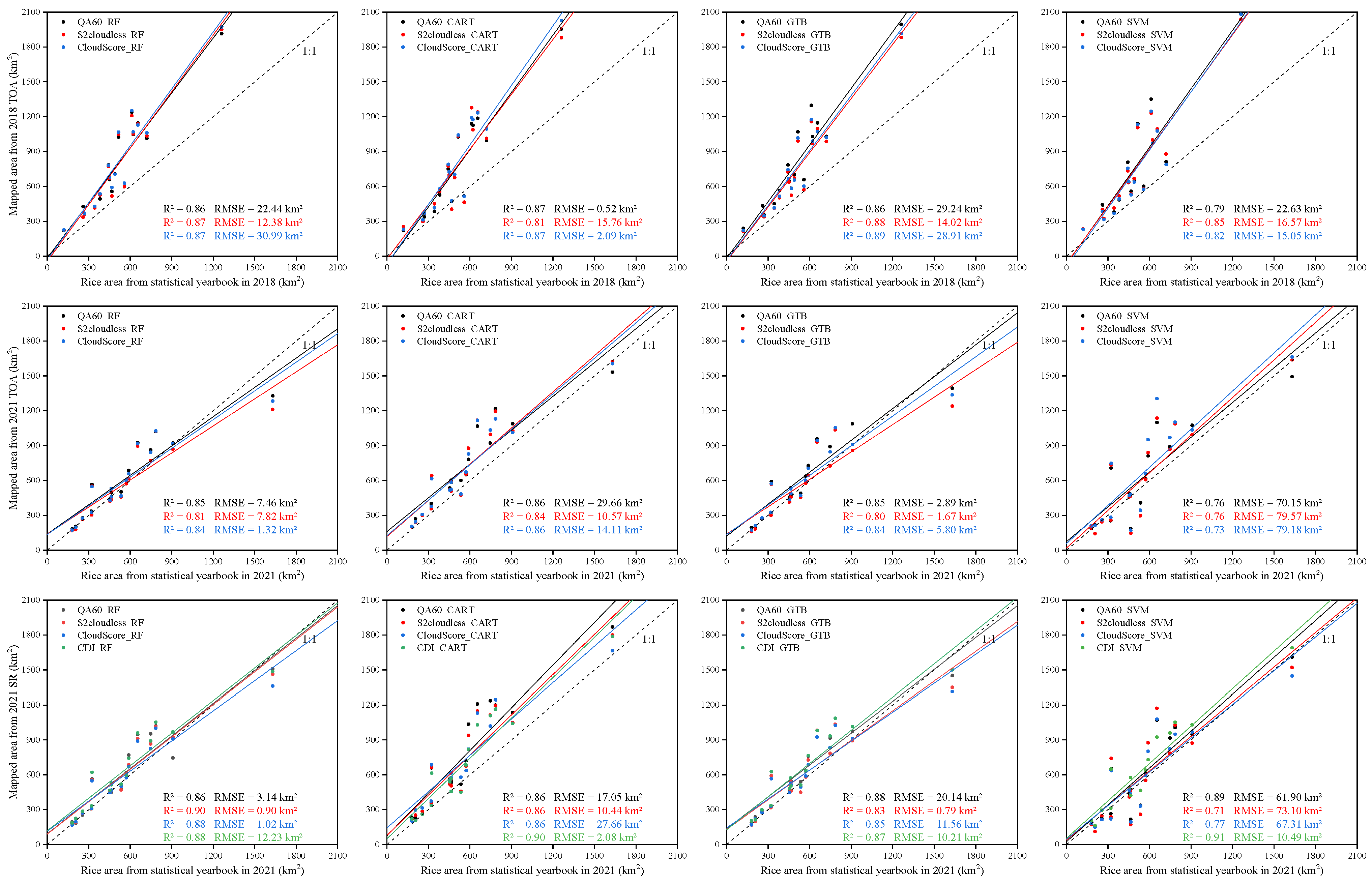
4.3.3. Comparing with Statistical Data

Rice-cropped areas derived from the statistical yearbook of the Hubei Province were compared with rice areas generated from our study in the JP based on a total of 16 counties. The statistical rice areas of the counties varied from 120.63 to 1261.11 km² in 2018 and 179.88 to 1629.87 km² in 2021. Generally, the mapped rice areas have high consistency with the county-level statistics. In the TOA products of 2018, the R² of all the comparisons is greater than 0.8 except for the comparison of rice area mapped from the QA60_SVM algorithm and the statistical area, and the comparison from the algorithm of QA60_CART has the smallest RMSE at 0.52 km². For the comparisons in the TOA products of 2021, rice areas mapped from SVM have comparatively smaller R² (<0.8) and larger RMSE (>75 km²) than those from RF, CART, and GTB. While in the comparison of 2021 SR products, SVM integrated with S2cloudless or CloudScore still had a relatively low R² (<0.8) and high RMSE (>65 km²), but showed a comparatively large R² (>0.9) and smaller RMSE (<11 km²) when combined with the CDI algorithm (Figure 9).

5. Discussion

5.1. Clear Observations after Cloud-Mask Processing

Focusing on the effect of cloud-mask algorithms on rice mapping, we adopted and compared four algorithms, including QA60, S2cloudless, CloudScore, and CDI, that are easy to operate in the GEE platform. From the result of Section 4.1, it can be concluded that S2cloudless showed the best performance in both accuracy assessment (OA = 97.04%) and visual inspection. CloudScore also proved to be a promising algorithm for masking clouds in the JP. Its OA was up to 94.82%, and both the entire and regional visual inspection results indicated a better cloud-mask outcome. Compared with S2cloudless and CloudScore, CDI and QA60 had relatively lower OAs (85% for CDI and 78.35 for QA60), and visual comparison findings were unsatisfactory from both a global and local perspective (Figure 4 and Figure 5). To further help us understand the effect of cloud removal from another viewpoint, clear observations (pixels) and their frequency after cloud removal were calculated based on the calendar month and the rice phenological stage (

Table 8. Percentages of clear observations masked by different cloud-mask algorithms in calendar months and rice phenological stages.

Period of Time	Cloud-Mask Algorithms	2018TOA						2021TOA						2021SR
		Effective Observation Element Frequency/%						Effective Observation Element Frequency/%						Effective Observation Element Frequency/%
		>0	(0, 20]	(20, 40]	(40, 60]	(60, 80]	(80, 100]	>0	(0, 20]	(20, 40]	(40, 60]	(60, 80]	(80, 100]	>0	(0, 20]	(20, 40]	(40, 60]	(60, 80]	(80, 100]
March	QA60	95.38	19.56	9.83	65.99	0.00	0.00	79.50	57.11	20.35	2.01	0.03	0.00	79.34	57.29	20.04	1.98	0.03	0.00
	S2cloudless	71.00	56.08	13.55	1.36	0.00	0.00	61.85	54.69	6.91	0.24	0.00	0.00	61.62	54.65	6.73	0.24	0.00	0.00
	CloudScore	86.44	61.06	22.78	2.59	0.00	0.00	66.71	55.28	10.65	0.76	0.01	0.00	70.21	53.79	15.00	1.39	0.02	0.00
	CDI	-	-	-	-	-	-	-	-	-	-	-	-	46.57	44.55	2.02	0.00	0.00	0.00
April	QA60	100.00	0.02	3.20	39.05	56.02	1.71	92.96	60.70	31.89	0.37	0.00	0.00	92.96	60.80	31.88	0.28	0.00	0.00
	S2cloudless	99.98	0.29	14.68	64.53	20.13	0.35	77.47	42.85	32.08	2.51	0.03	0.00	77.45	42.92	32.11	2.38	0.03	0.00
	CloudScore	99.31	0.66	4.66	51.95	38.61	3.41	93.08	31.61	53.31	7.54	0.61	0.00	95.68	23.41	60.48	11.02	0.75	0.01
	CDI	-	-	-	-	-	-	-	-	-	-	-	-	50.01	44.31	5.55	0.15	0.00	0.00
May	QA60	97.44	15.12	36.12	35.59	10.61	0.00	79.13	33.79	36.02	9.07	0.25	0.00	78.99	33.68	36.14	8.93	0.24	0.00
	S2cloudless	95.71	14.96	36.24	38.17	6.33	0.01	82.55	32.68	39.23	10.59	0.05	0.00	82.51	32.67	39.37	10.42	0.04	0.00
	CloudScore	95.70	10.47	32.22	44.15	8.77	0.07	88.45	21.97	31.81	30.95	3.71	0.01	95.89	17.81	33.61	40.02	4.44	0.02
	CDI	-	-	-	-	-	-	-	-	-	-	-	-	70.15	42.88	23.61	3.66	0.00	0.00
June	QA60	96.81	11.25	35.65	45.03	4.88	0.00	100.00	8.67	46.54	32.93	10.78	1.08	100.00	8.73	46.62	32.79	10.79	1.07
	S2cloudless	96.04	16.02	43.34	35.87	0.81	0.00	99.94	23.41	44.92	26.63	4.88	0.10	99.94	23.53	44.95	26.49	4.87	0.10
	CloudScore	97.70	9.14	38.79	46.49	3.27	0.00	98.61	15.36	37.13	35.37	9.63	1.11	99.34	9.62	32.23	42.89	13.04	1.54
	CDI	-	-	-	-	-	-	-	-	-	-	-	-	99.98	72.58	24.53	2.80	0.07	0.00
July	QA60	99.92	27.35	46.92	20.78	4.87	0.00	99.99	3.43	49.77	46.77	0.02	0.00	99.99	3.53	49.77	46.68	0.01	0.00
	S2cloudless	99.42	20.03	43.91	31.40	4.07	0.00	99.74	7.66	53.42	38.61	0.05	0.00	99.74	7.81	53.33	38.55	0.05	0.00
	CloudScore	99.01	7.31	29.37	55.67	6.65	0.00	99.13	5.34	44.93	48.32	0.52	0.01	99.46	3.83	38.45	56.01	1.15	0.02
	CDI	-	-	-	-	-	-	-	-	-	-	-	-	92.41	44.70	39.48	8.23	0.00	0.00
August	QA60	99.98	0.83	6.18	21.45	30.88	40.64	99.58	12.44	47.20	39.88	0.06	0.00	99.57	12.52	47.24	39.80	0.01	0.00
	S2cloudless	98.75	11.13	18.63	29.67	22.50	16.82	96.67	14.91	44.73	36.73	0.29	0.00	96.64	14.94	44.81	36.66	0.23	0.00
	CloudScore	98.91	5.71	12.83	26.24	26.11	28.00	97.91	12.19	38.17	46.83	0.71	0.00	98.74	9.95	35.41	51.65	1.72	0.00
	CDI	-	-	-	-	-	-	-	-	-	-	-	-	85.76	41.17	41.00	3.58	0.01	0.00
September	QA60	90.94	58.74	28.87	3.32	0.01	0.00	100.00	0.03	1.62	23.97	32.95	41.43	100.00	0.03	1.65	24.07	33.08	41.17
	S2cloudless	84.95	65.28	18.96	0.70	0.01	0.00	99.98	0.15	2.85	23.54	29.96	43.48	99.98	0.15	2.85	23.58	29.98	43.42
	CloudScore	85.36	62.00	22.06	1.28	0.01	0.00	99.47	0.64	2.72	20.95	28.03	47.13	99.69	0.35	1.62	18.50	28.96	50.25
	CDI	-	-	-	-	-	-	-	-	-	-	-	-	99.74	3.15	17.20	31.81	26.54	21.04
October	QA60	99.54	2.64	32.29	61.82	2.79	0.00	100.00	4.56	85.98	9.41	0.05	0.00	100.00	4.66	86.07	9.23	0.04	0.00
	S2cloudless	99.92	1.77	28.12	68.21	1.81	0.00	99.96	4.00	89.46	6.41	6.03	0.08	99.96	4.14	89.51	6.22	0.08	0.00
	CloudScore	99.45	1.97	23.21	70.77	3.48	0.01	99.02	3.72	89.94	5.35	0.00	0.00	99.61	1.46	89.38	8.75	0.01	0.00
	CDI	-	-	-	-	-	-	-	-	-	-	-	-	99.99	7.63	91.02	1.33	0.00	0.00
Bare soil stage	QA60	100.00	0.82	19.54	73.81	5.83	0.00	97.96	36.11	57.52	4.32	0.01	0.00	97.75	35.97	57.54	4.23	0.00	0.00
03/20–04/20	S2cloudless	99.98	0.48	17.77	79.89	1.84	0.00	88.24	35.38	46.89	5.73	0.24	0.00	88.22	35.44	46.86	5.69	0.22	0.00
	CloudScore	99.25	0.70	6.04	84.53	7.98	0.00	96.87	21.53	59.69	14.66	0.98	0.01	99.08	14.77	63.79	18.49	1.99	0.04
	CDI	-	-	-	-	-	-	-	-	-	-	-	-	62.98	46.10	16.74	0.14	0.00	0.00
Transplanting stage	QA60	99.98	4.23	38.74	51.77	5.24	0.00	100.00	23.64	61.28	14.65	0.43	0.00	100.00	23.70	61.43	14.45	0.42	0.00
04/20–06/15	S2cloudless	99.09	13.10	53.51	32.05	0.43	0.00	99.96	29.72	58.43	11.73	0.08	0.00	99.96	29.75	58.60	11.53	0.08	0.00
	CloudScore	95.56	3.23	46.53	44.37	1.43	0.00	96.79	16.03	48.42	31.50	0.83	0.00	99.59	8.00	48.31	41.96	1.31	0.00
	CDI	-	-	-	-	-	-	-	-	-	-	-	-	99.99	60.56	37.45	1.98	0.00	0.00
Growth stage	QA60	100.00	0.17	25.55	68.10	6.18	0.00	100.00	1.85	70.21	27.66	0.28	0.00	100.00	1.91	70.26	27.56	0.27	0.00
06/15–09/10	S2cloudless	99.99	3.95	48.07	45.09	2.88	0.00	99.99	9.43	61.59	28.88	0.08	0.00	99.99	9.48	61.66	28.76	0.08	0.00
	CloudScore	99.59	1.66	23.45	65.42	9.06	0.00	99.67	5.72	49.71	42.83	1.41	0.00	99.81	2.78	42.92	52.12	1.99	0.00
	CDI	-	-	-	-	-	-	-	-	-	-	-	-	92.17	35.52	42.99	13.66	0.00	0.00
Harvest stage	QA60	100.00	3.67	81.12	14.90	0.31	0.00	100.00	0.00	0.45	92.90	6.65	0.00	100.00	0.00	0.56	92.84	6.59	0.00
09/10–10/25	S2cloudless	99.97	6.48	84.45	8.95	0.09	0.00	99.98	0.02	2.15	96.04	1.76	0.00	99.98	0.02	2.30	95.89	1.76	0.00
	CloudScore	99.38	5.81	72.02	21.41	0.14	0.00	99.34	0.37	2.33	92.67	3.97	0.00	99.67	0.23	1.24	90.98	7.22	0.00
	CDI	-	-	-	-	-	-	-	-	-	-	-	-	99.99	0.03	16.09	83.65	0.22	0.00

). Thus, we could determine the number (or proportion) of clear pixels that might be used for mapping rice after the cloud-mask procedure.

As shown in Table 8, clear observation frequency (COF, defined as the ratio of clear observation to total observation) greater than 0 has a high percentage (>85%) in each calendar month from March to October, except 71% of S2cloudless in March of 2018. Hence, when the time scale changed into phenological stages of paddy rice, the percentage of COF > 0 increased to more than 95% in 2018. It indicated that nearly every pixel had at least one clear observation at each phenological stage in the JP while using the four cloud-mask algorithms. However, it was difficult to map rice in a cloud-prone region when each pixel had only one clear observation within each phenological stage. Therefore, we separated COF into five ranges (0–20%, 20–40%, 40–60%, 60–80%, and 80–100%) and calculated the percentage of COF in each category. For TOA products in 2018, the largest proportion of COF spread in different ranges, varying with the cloud-mask algorithm during different calendar months and phenological stages. Yet, it had high consistency in September and October, as well as the bare soil stage and harvest stage. The percentages of COF between 40 and 60% were larger than 70% in the bare soil stage and harvest stage, which implied spectral signatures of these phenological stages in rice paddy could be used for mapping rice in 2018. If we combine the second largest percentages of COF with the first largest percentages, more than 90% of the pixels contain 20–60% clear observations during the bare soil and harvest stage that could be used for rice mapping. Likewise, rice mapping could be facilitated by the fact that over 85% of pixels had 20–60% unambiguous observations at the transplanting and growing stages.

The COF of 2021 TOA products showed somewhat different statistics from the COF of 2018 TOA products while having great consistency with the COF of 2021 SR products. From the view of the calendar month of 2018 TOA products, the largest percentages of COF were placed into the ranges of 0–20% in March, the ranges of 20–40% in May, June, and October, and the ranges of 80–100% in September. When the second largest proportions were merged with the largest proportions at phenological stages, the statistical results showed that over 80% of pixels had 0–40% clear observations in the bare soil stages, and this percentage would climb over 90% in the range of 20–60% in the growing stage. The variation of COF in the bare soil stage and the similarity of COF in the growing stage of 2023 when compared to the 2018 TOA products indicated that the effects of the three cloud-mask algorithms operating in separate years were diverse for different phenological stages of paddy rice. For the transplanting stage commonly used in previous studies, the combination of the largest and the second largest proportion of COF were positioned in the range of 20–60% by QA60 and S2cloudless in 2018, compared with the range of 0–40% by these algorithms in 2021. This meant there were some variations between the two algorithms’ cloud removal performance in 2018 and 2021, while CloudScore demonstrated good stability between these years as its combined proportions (the largest and the second largest) were steady within the range of 20–60%.

5.2. Combination of Cloud-Mask Algorithm and Machine-Learning Algorithms Used for Rice Mapping

To thoroughly assess the GEE-embedded algorithms used for rice mapping in the cloud-prone area, four cloud-mask algorithms and four machine-learning algorithms were integrated. Although all of the machine-learning algorithms fall into the category of supervised classification methods, different performances were observed when the four classifiers were used to classify the dataset that had been cloud-masked by the same algorithm. For the accuracy assessment, S2cloudless combined with RF showed overwhelming dominance in OA and PA/UA of paddy rice than other combinations (Table 7). In the comparisons of Jaccard similarity, S2cloudless_GTB, and S2cloudless_RF, as well as S2cloudless_RF and CloudScore_RF were the first two combinations with high similarity in the datasets of 2018 and 2021 (Figure 8). However, no algorithm combination can achieve consistently high accuracy in the comparisons of statistical data in TOA products. The combination of RF and four cloud-mask algorithms showed an overall larger R² than other algorithm combinations in the comparison of statistical data over SR products. Thus, it can be seen that S2cloudless_RF and CloudScore_RF demonstrated an overall advantage over other algorithm combinations.

Combined with the analysis of COF in Section 5.1, it needs to be pointed out that paddy rice mapping of remote sensing based on its phenological stages may be different from that based on calendar month because the cloud-free observations varied between the two time scales depending on the cloud-mask algorithms. The clear observation used for mapping rice could be dramatically changed when the time scale switched from calendar month to rice phenological stages. For example, the largest proportion of COF by CloudScore changed from 61.06% in the range of 0–20% in March to 84.53% in the range of 40–60% in the bare soil stage of 2018. Another issue that should not be ignored is that the authenticity of cloud-mask algorithms and their combination with classifiers should receive attention, even though COF could be used as a crucial metric for assessing cloud-mask algorithms and have a direct impact on the accuracy of rice mapping. For example, the transplanting stage was recognized as a critical stage in mapping rice, and QA60 had a larger proportion of COF in the range of 40–60% than S2cloudless and CloudScore during this phenological stage in 2018. However, QA60-classifier combinations do not have the best accuracy in rice mapping. For example, in the 2018 TOA products, the largest OA was 90.15% in QA60_RF, compared with 92.06% in S2cloudless_RF. In the visual inspection of the cloud removal of QA60, it was found that some cloud pixels would be retained for the mapping. Meanwhile, QA60 had a slightly higher proportion of COF in the range of 20–40% than S2cloudless (57.52% vs. 46.89%, 61.28% vs. 58.43%, 70.21% vs. 61.59%) in the three stages (bare soil stage, transplanting stage, and growing stage) of 2021 TOA products, but both OA and paddy rice’s PA of S2cloudless-classifier combinations were larger than that of QA60-classifier combinations. Admittedly, the COF of other phenological stages may also have an impact on the mapping accuracy, the reliability of various cloud-mask algorithms and the robustness of their combinations of classifiers are of greater significance in rice mapping.

5.3. Limitations and Implications of the Study

Remote sensing mapping of paddy rice is susceptible to cloud-contaminated pixels in rice cropping areas, and the study of cloud-mask algorithms has been a popular topic in this field. Due to the widespread use of Sentinel-2 imagery in many different fields, a few cloud-mask algorithms, such as ATCOR [28], Fmask [55,56,57], MAJA [56,57], Sen2Cor [56,57], etc., have been quickly developed in various frameworks and tested in a variety of environments. It is inconvenient to use these processors because they run in separate contexts and require cross-platform operations for rice mapping. In contrast to the earlier research on the mechanism of the cloud-mask algorithm (they used standard imagery dataset to test cloud-mask algorithms across different software platforms), one of the goals of this study was intended to evaluate the GEE-embedded cloud-mask algorithms for rice mapping. As a result, the mapping process can be conducted on the GEE platform, reducing the complex process of data conversion caused by cross-platform. Moreover, a survey of the literature revealed that the data preparation step in most rice mapping research employing Sentinel-2 data was highly dependent on the QA60 band for recognizing clouds and cloud shadows [15]. Then, they mapped paddy rice with various machine-learning algorithms based on QA60-masked images. In our study, after comparing four GEE-embedded cloud-mask algorithms, we analyzed the appropriateness of four popular machine-learning algorithms for cloud-masked Sentinel-2 imagery in mapping paddy rice. The second aim of the study was to suggest an appropriate strategy for the combinations of cloud-mask algorithms and machine-learning algorithms for rice mapping in subtropical areas on the GEE platform. This is a completely distinct concept from earlier research that used global reference datasets to assess cloud-mask algorithms, such as Cloud Masking Intercomparison eXercise (CMIX) [26]. For further research, integrating multiple cloud-mask algorithms into a cloud platform and developing crop-specific cloud-mask mapping schemes is of great essence in crop mapping.

6. Conclusions

Mapping paddy rice with optical remotely sensing imagery in cloud-prone regions faces a lot of challenges. In this study, we compared and evaluated four GEE-embedded cloud-mask algorithms in Sentinel-2 imagery and integrated them with four commonly used machine-learning algorithms for rice mapping in a traditional rice cropping area of southern China. Generally, S2cloudless showed the best performance in cloud removal with the largest OA of 97.06%, and the cloud-mask algorithms performed better in SR products than TOA products of Sentinel-2 imagery. The combinations of S2cloudless and RF showed a dominant performance in OA and PA/UA of paddy rice compared to other combinations. Although clear observations in the key phenological stages are crucial for rice mapping, the authenticity of cloud-mask algorithms and their integration with classifiers should receive more attention. The strategy proposed in this study for mapping paddy rice can be extended into other cloudy regions to provide precise agricultural information for the sustainable development of agricultural practices.

References

1. Wheeler, T.; Von Braun, J. Climate change impacts on global food security. Science 2013, 341, 508–513. [Google Scholar] [CrossRef]
2. Fuller, D.Q.; Qin, L.; Zheng, Y.; Zhao, Z.; Chen, X.; Hosoya, L.A.; Sun, G.P. The domestication process and domestication rate in rice: Spikelet bases from the Lower Yangtze. Science 2009, 323, 1607–1610. [Google Scholar] [CrossRef] [PubMed]
3. Dong, J.; Xiao, X.; Menarguez, M.A.; Zhang, G.; Qin, Y.; Thau, D.; Biradar, C.; Moore, B., III. Mapping paddy rice planting area in northeastern Asia with Landsat 8 images, phenology-based algorithm and Google Earth Engine. Remote Sens. Environ. 2016, 185, 142–154. [Google Scholar] [CrossRef] [PubMed]
4. Xin, F.; Xiao, X.; Dong, J.; Zhang, G.; Zhang, Y.; Wu, X.; Li, X.; Zou, Z.; Ma, J.; Du, G.; et al. Large increases of paddy rice area, gross primary production, and grain production in Northeast China during 2000–2017. Sci. Total Environ. 2020, 711, 135183. [Google Scholar] [CrossRef] [PubMed]
5. Zhang, G.; Xiao, X.; Biradar, C.M.; Dong, J.; Qin, Y.; Menarguez, M.A.; Zhou, Y.; Zhang, Y.; Jin, C.; Wang, J.; et al. Spatiotemporal patterns of paddy rice croplands in China and India from 2000 to 2015. Sci. Total Environ. 2017, 579, 82–92. [Google Scholar] [CrossRef] [PubMed]
6. Wang, H.; Shao, Q.; Li, R.; Song, M.; Zhou, Y. Governmental policies drive the LUCC trajectories in the Jianghan Plain. Environ. Monit. Assess. 2013, 185, 10521–10536. [Google Scholar] [CrossRef] [PubMed]
7. Xiao, X.; Boles, S.; Liu, J.; Zhuang, D.; Frolking, S.; Li, C.; Salas, W.; Moore, B., III. Mapping paddy rice agriculture in southern China using multi-temporal MODIS images. Remote Sens. Environ. 2005, 95, 480–492. [Google Scholar] [CrossRef]
8. Zhang, X.; Wu, B.; Ponce-Campos, G.E.; Zhang, M.; Chang, S.; Tian, F. Mapping up-to-date paddy rice extent at 10 m resolution in china through the integration of optical and synthetic aperture radar images. Remote Sens. 2018, 10, 1200. [Google Scholar] [CrossRef]
9. Liu, L.; Xiao, X.; Qin, Y.; Wang, J.; Xu, X.; Hu, Y.; Qiao, Z. Mapping cropping intensity in China using time series Landsat and Sentinel-2 images and Google Earth Engine. Remote Sens. Environ. 2020, 239, 111624. [Google Scholar] [CrossRef]
10. Cao, J.; Cai, X.; Tan, J.; Cui, Y.; Xie, H.; Liu, F.; Yang, L.; Luo, Y. Mapping paddy rice using Landsat time series data in the Ganfu Plain irrigation system, Southern China, from 1988- 2017. Int. J. Remote Sens. 2021, 42, 1556–1576. [Google Scholar] [CrossRef]
11. Ni, R.; Tian, J.; Li, X.; Yin, D.; Li, J.; Gong, H.; Zhang, J.; Zhu, L.; Wu, D. An enhanced pixel-based phenological feature for accurate paddy rice mapping with Sentinel-2 imagery in Google Earth Engine. ISPRS J. Photogramm. Remote Sens. 2021, 178, 282–296. [Google Scholar] [CrossRef]
12. Dong, J.; Xiao, X.; Kou, W.; Qin, Y.; Zhang, G.; Li, L.; Jin, C.; Zhou, Y.; Wang, J.; Biradar, C.; et al. Tracking the dynamics of paddy rice planting area in 1986–2010 through time series Landsat images and phenology-based algorithms. Remote Sens. Environ. 2015, 160, 99–113. [Google Scholar] [CrossRef]
13. Boschetti, M.; Busetto, L.; Manfron, G.; Laborte, A.; Asilo, S.; Pazhanivelan, S.; Nelson, A. PhenoRice: A method for automatic extraction of spatio-temporal information on rice crops using satellite data time series. Remote Sens. Environ. 2017, 194, 347–365. [Google Scholar] [CrossRef]
14. Xu, S.; Zhu, X.; Chen, J.; Zhu, X.; Duan, M.; Qiu, B.; Wan, L.; Tan, X.; Xu, Y.N.; Cao, R. A robust index to extract paddy fields in cloudy regions from SAR time series. Remote Sens. Environ. 2023, 285, 113374. [Google Scholar] [CrossRef]
15. He, Y.; Dong, J.; Liao, X.; Sun, L.; Wang, Z.; You, N.; Li, Z.; Fu, P. Examining rice distribution and cropping intensity in a mixed single-and double-cropping region in South China using all available Sentinel 1/2 images. Int. J. Appl. Earth Obs. Geoinf. 2021, 101, 102351. [Google Scholar] [CrossRef]
16. Peng, D.; Huete, A.R.; Huang, J.; Wang, F.; Sun, H. Detection and estimation of mixed paddy rice cropping patterns with MODIS data. Int. J. Appl. Earth Obs. Geoinf. 2011, 13, 13–23. [Google Scholar] [CrossRef]
17. Fritz, S.; See, L.; McCallum, I.; You, L.; Bun, A.; Moltchanova, E.; Duerauer, M.; Albrecht, F.; Schill, C.; Perger, C.; et al. Mapping global cropland and field size. Glob. Chang. Biol. 2015, 21, 1980–1992. [Google Scholar] [CrossRef] [PubMed]
18. Phiri, D.; Simwanda, M.; Salekin, S.; Nyirenda, V.R.; Murayama, Y.; Ranagalage, M. Sentinel-2 data for land cover/use mapping: A review. Remote Sens. 2020, 12, 2291. [Google Scholar] [CrossRef]
19. Chen, N.; Yu, L.; Zhang, X.; Shen, Y.; Zeng, L.; Hu, Q.; Niyogi, D. Mapping paddy rice fields by combining multi-temporal vegetation index and synthetic aperture radar remote sensing data using google earth engine machine learning platform. Remote Sens. 2020, 12, 2992. [Google Scholar] [CrossRef]
20. Inoue, S.; Ito, A.; Yonezawa, C. Mapping Paddy fields in Japan by using a Sentinel-1 SAR time series supplemented by Sentinel-2 images on Google Earth Engine. Remote Sens. 2020, 12, 1622. [Google Scholar] [CrossRef]
21. Karimi, N.; Taban, M.R. A convex variational method for super resolution of SAR image with speckle noise. Signal Process. Image Commun. 2021, 90, 116061. [Google Scholar] [CrossRef]
22. Zhan, P.; Zhu, W.; Li, N. An automated rice mapping method based on flooding signals in synthetic aperture radar time series. Remote Sens. Environ. 2021, 252, 112112. [Google Scholar] [CrossRef]
23. Zhu, Z.; Wang, S.; Woodcock, C.E. Improvement and expansion of the Fmask algorithm: Cloud, cloud shadow, and snow detection for Landsats 4–7, 8, and Sentinel 2 images. Remote Sens. Environ. 2015, 159, 269–277. [Google Scholar] [CrossRef]
24. Foga, S.; Scaramuzza, P.L.; Guo, S.; Zhu, Z.; Dilley, R.D., Jr.; Beckmann, T.; Schmidt, G.L.; Dwyer, J.L.; Hughes, M.J.; Laue, B. Cloud detection algorithm comparison and validation for operational Landsat data products. Remote Sens. Environ. 2017, 194, 379–390. [Google Scholar] [CrossRef]
25. Mateo-García, G.; Gómez-Chova, L.; Amorós-López, J.; Muñoz-Marí, J.; Camps-Valls, G. Multitemporal cloud masking in the Google Earth Engine. Remote Sens. 2018, 10, 1079. [Google Scholar] [CrossRef]
26. Skakun, S.; Wevers, J.; Brockmann, C.; Doxani, G.; Aleksandrov, M.; Batič, M.; Frantz, D.; Gascon, F.; Gómez-Chova, L.; Hagolle, O.; et al. Cloud Mask Intercomparison eXercise (CMIX): An evaluation of cloud masking algorithms for Landsat 8 and Sentinel-2. Remote Sens. Environ. 2022, 274, 112990. [Google Scholar] [CrossRef]
27. Frantz, D.; Haß, E.; Uhl, A.; Stoffels, J.; Hill, J. Improvement of the Fmask algorithm for Sentinel-2 images: Separating clouds from bright surfaces based on parallax effects. Remote Sens. Environ. 2018, 215, 471–481. [Google Scholar] [CrossRef]
28. Zekoll, V.; Main-Knorn, M.; Alonso, K.; Louis, J.; Frantz, D.; Richter, R.; Pflug, B. Comparison of masking algorithms for sentinel-2 imagery. Remote Sens. 2021, 13, 137. [Google Scholar] [CrossRef]
29. Mullissa, A.; Vollrath, A.; Odongo-Braun, C.; Slagter, B.; Balling, J.; Gou, Y.; Gorelick, N.; Reiche, J. Sentinel-1 sar backscatter analysis ready data preparation in google earth engine. Remote Sens. 2021, 13, 1954. [Google Scholar] [CrossRef]
30. Zupanc, A. Improving Cloud Detection with Machine Learning. Available online: https://medium.com/sentinel-hub/improving-cloud-detection-with-machine-learning-c09dc5d7cf13 (accessed on 24 March 2024).
31. Housman, I.W.; Chastain, R.A.; Finco, M.V. An evaluation of forest health insect and disease survey data and satellite-based remote sensing forest change detection methods: Case studies in the United States. Remote Sens. 2018, 10, 1184. [Google Scholar] [CrossRef]
32. Chastain, R.; Housman, I.; Goldstein, J.; Finco, M.; Tenneson, K. Empirical cross sensor comparison of Sentinel-2A and 2B MSI, Landsat-8 OLI, and Landsat-7 ETM+ top of atmosphere spectral characteristics over the conterminous United States. Remote Sens. Environ. 2019, 221, 274–285. [Google Scholar] [CrossRef]
33. Wang, C.; Wang, G.; Zhang, G.; Cui, Y.; Zhang, X.; He, Y.; Zhou, Y. Freshwater Aquaculture Mapping in “Home of Chinese Crawfish” by Using a Hierarchical Classification Framework and Sentinel-1/2 Data. Remote Sens. 2024, 16, 893. [Google Scholar] [CrossRef]
34. Wu, B.; Li, Q. Crop planting and type proportion method for crop acreage estimation of complex agricultural landscapes. Int. J. Appl. Earth Obs. Geoinf. 2012, 16, 101–112. [Google Scholar] [CrossRef]
35. Shen, R.; Pan, B.; Peng, Q.; Dong, J.; Chen, X.; Zhang, X.; Ye, T.; Huang, J.; Yuan, W. High-resolution distribution maps of single-season rice in China from 2017 to 2022. Earth Syst. Sci. Data Discuss. 2023, 15, 3203–3222. [Google Scholar] [CrossRef]
36. Weigand, M.; Staab, J.; Wurm, M.; Taubenböck, H. Spatial and semantic effects of LUCAS samples on fully automated land use/land cover classification in high-resolution Sentinel-2 data. Int. J. Appl. Earth Obs. Geoinf. 2020, 88, 102065. [Google Scholar] [CrossRef]
37. Zhu, W.; Peng, X.; Ding, M.; Li, L.; Liu, Y.; Liu, W.; Yang, M.; Chen, X.; Cai, J.; Huang, H.; et al. Decline in Planting Areas of Double-Season Rice by Half in Southern China over the Last Two Decades. Remote Sens. 2024, 16, 440. [Google Scholar] [CrossRef]
38. Chu, L.; Jiang, C.; Wang, T.; Li, Z.; Cai, C. Mapping and forecasting of rice cropping systems in central China using multiple data sources and phenology-based time-series similarity measurement. Adv. Space Res. 2021, 68, 3594–3609. [Google Scholar] [CrossRef]
39. Thorp, K.; Drajat, D. Deep machine learning with Sentinel satellite data to map paddy rice production stages across West Java, Indonesia. Remote Sens. Environ. 2021, 265, 112679. [Google Scholar] [CrossRef]
40. Bera, B.; Saha, S.; Bhattacharjee, S. Estimation of forest canopy cover and forest fragmentation mapping using Landsat satellite data of Silabati River Basin (India). KN J. Cartogr. Geogr. Inf 2020, 70, 181–197. [Google Scholar] [CrossRef]
41. Tucker, C.J. Red and photographic infrared linear combinations for monitoring vegetation. Remote Sens. Environ. 1979, 8, 127–150. [Google Scholar] [CrossRef]
42. Huete, A.; Liu, H.; Batchily, K.; Van Leeuwen, W. A comparison of vegetation indices over a global set of TM images for EOS-MODIS. Remote Sens. Environ. 1997, 59, 440–451. [Google Scholar] [CrossRef]
43. Merzlyak, M.N.; Gitelson, A.A.; Chivkunova, O.B.; Rakitin, V.Y. Non-destructive optical detection of pigment changes during leaf senescence and fruit ripening. Physiol. Plant. 1999, 106, 135–141. [Google Scholar] [CrossRef]
44. Dash, J.; Jeganathan, C.; Atkinson, P. The use of MERIS Terrestrial Chlorophyll Index to study spatio-temporal variation in vegetation phenology over India. Remote Sens. Environ. 2010, 114, 1388–1402. [Google Scholar] [CrossRef]
45. Wang, Y.; Gong, Z.; Zhou, H. Long-term monitoring and phenological analysis of submerged aquatic vegetation in a shallow lake using time-series imagery. Ecol. Indic. 2023, 154, 110646. [Google Scholar] [CrossRef]
46. Li, K.; Chen, Y. A Genetic Algorithm-based urban cluster automatic threshold method by combining VIIRS DNB, NDVI, and NDBI to monitor urbanization. Remote Sens. 2018, 10, 277. [Google Scholar] [CrossRef]
47. Breiman, L. Random forests. Mach. Learn. 2001, 45, 5–32. [Google Scholar] [CrossRef]
48. Mansaray, L.R.; Kanu, A.S.; Yang, L.; Huang, J.; Wang, F. Evaluation of machine learning models for rice dry biomass estimation and mapping using quad-source optical imagery. GISci. Remote Sens. 2020, 57, 785–796. [Google Scholar] [CrossRef]
49. Aghighi, H.; Azadbakht, M.; Ashourloo, D.; Shahrabi, H.S.; Radiom, S. Machine learning regression techniques for the silage maize yield prediction using time-series images of Landsat 8 OLI. IEEE J. Sel. Top. Appl. Earth Obs. Remote Sens. 2018, 11, 4563–4577. [Google Scholar] [CrossRef]
50. Abdi, A.M. Land cover and land use classification performance of machine learning algorithms in a boreal landscape using Sentinel-2 data. GISci. Remote Sens. 2020, 57, 1–20. [Google Scholar] [CrossRef]
51. Tolpekin, V.A.; Stein, A. Quantification of the effects of land-cover-class spectral separability on the accuracy of Markov-random-field-based superresolution mapping. IEEE Trans. Geosci. Remote Sens. 2009, 47, 3283–3297. [Google Scholar] [CrossRef]
52. Wang, Y.; Qi, Q.; Liu, Y. Unsupervised segmentation evaluation using area-weighted variance and Jeffries-Matusita distance for remote sensing images. Remote Sens. 2018, 10, 1193. [Google Scholar] [CrossRef]
53. Schmidt, K.; Skidmore, A. Spectral discrimination of vegetation types in a coastal wetland. Remote Sens. Environ. 2003, 85, 92–108. [Google Scholar] [CrossRef]
54. Jaccard, P. The distribution of the flora in the alpine zone. 1. New Phytol. 1912, 11, 37–50. [Google Scholar] [CrossRef]
55. Qiu, S.; Zhu, Z.; He, B. Fmask 4.0: Improved cloud and cloud shadow detection in Landsats 4–8 and Sentinel-2 imagery. Remote Sens. Environ. 2019, 231, 111205. [Google Scholar] [CrossRef]
56. Sanchez, A.H.; Picoli, M.C.A.; Camara, G.; Andrade, P.R.; Chaves, M.E.D.; Lechler, S.; Soares, A.R.; Marujo, R.F.; Simões, R.E.O.; Ferreira, K.R.; et al. Comparison of Cloud cover detection algorithms on sentinel–2 images of the amazon tropical forest. Remote Sens. 2020, 12, 1284. [Google Scholar] [CrossRef]
57. Baetens, L.; Desjardins, C.; Hagolle, O. Validation of copernicus Sentinel-2 cloud masks obtained from MAJA, Sen2Cor, and FMask processors using reference cloud masks generated with a supervised active learning procedure. Remote Sens. 2019, 11, 433. [Google Scholar] [CrossRef]
Figure 1. Overview map of the study area. The grids are Sentinel-2 footprints in MGRS (Military Grid Reference System) with an area of 100 km × 100 km square. Land cover data was from the optimal mapping results of this study.
Remotesensing 16 01305 g001
Figure 2. The workflow of the study included data preprocessing and cloud mask algorithm evaluation, sample selection and feature selection, extraction of rice phenology and image compositing, comparisons of machine-learning algorithms in rice mapping and validation of rice maps (validation of field data samples, comparison of 10 m rice maps, and comparison of statistical data).
Remotesensing 16 01305 g002
Figure 3. Paddy rice phenological stages derived from the fitted curves of five spectral indices based on the cloud-masked TOA dataset in 2021 (field photographs were taken at 112 . 8804 E, 30 . 0690 N).
Remotesensing 16 01305 g003
Figure 4. Results of four cloud-mask algorithms in the tile of 49REP, 49RFP, and 49RGP (the specific locations of these footprints in the study area are shown in Figure 1). Each row shows the cloud identification results based on 49REP’s May 2018 TOA data, 49RFP’s July 2021 TOA data, and 49RGP’s September 2021 SR data using QA60, S2cloudless, CloudScore, and CDI cloud mask algorithms, respectively.
Remotesensing 16 01305 g004
Figure 5. Results of four cloud-mask algorithms in three subregions across the tiles of 49REP, 49RFP, and 49RGP with different land cover characteristics. Panels a, b, and c show the results in a region mixed with built-up area and paddy rice, a region mixed with dryland and paddy rice, and a region mixed with paddy rice and aquaculture area, respectively.
Remotesensing 16 01305 g005
Figure 6. J-M values of paddy rice and other land cover types to cloud-free datasets for different cloud-mask algorithms.
Remotesensing 16 01305 g006
Figure 7. Percentages of the specified land cover area to the total area in different land cover types were estimated from the different combinations of cloud-mask algorithms and machine-learning algorithms. The bars show the percentage in area of water body, built-up area, forest land, dryland, and paddy rice from left to right, respectively.
Remotesensing 16 01305 g007
Figure 8. J-sim values between the reference rice maps and the maps generated from different algorithm combinations.
Remotesensing 16 01305 g008
Figure 9. Comparisons of rice area between statistical data and mapping results.
Remotesensing 16 01305 g009