Article

Characterizing the California Current System through Sea Surface Temperature and Salinity

by
Marisol García-Reyes
1,*,
Gammon Koval
1 and
Jorge Vazquez-Cuervo
2
1
Farallon Institute, Petaluma, CA 94952, USA
2
Jet Propulsion Laboratory, California Institute of Technology, Pasadena, CA 91109, USA
*
Author to whom correspondence should be addressed.
Remote Sens. 2024, 16(8), 1311; https://doi.org/10.3390/rs16081311
Submission received: 23 January 2024 / Revised: 28 March 2024 / Accepted: 4 April 2024 / Published: 9 April 2024

Abstract

:
Characterizing temperature and salinity (T-S) conditions is a standard framework in oceanography to identify and describe deep water masses and their dynamics. At the surface, this practice is hindered by multiple air–sea–land processes impacting T-S properties at shorter time scales than can easily be monitored. Now, however, the unsurpassed spatial and temporal coverage and resolution achieved with satellite sea surface temperature (SST) and salinity (SSS) allow us to use these variables to investigate the variability of surface processes at climate-relevant scales. In this work, we use SSS and SST data, aggregated into domains using a cluster algorithm over a T-S diagram, to describe the surface characteristics of the California Current System (CCS), validating them with in situ data from uncrewed Saildrone vessels. Despite biases and uncertainties in SSS and SST values in highly dynamic coastal areas, this T-S framework has proven useful in describing CCS regional surface properties and their variability in the past and in real time, at novel scales. This analysis also shows the capacity of remote sensing data for investigating variability in land–air–sea interactions not previously possible due to limited in situ data.

1. Introduction

Temperature and salinity are fundamental ocean variables in both physical and biological marine science. At depth, they describe water masses’ properties, including density, and therefore have been widely used in oceanography to describe ocean currents and mixing at regional and global scales, which in turn influence the transport of other ocean properties like heat, nutrients, and carbon [1]. To identify different water masses, water conditions are plotted in temperature and salinity space, referred to as a T-S diagram, where salinity is plotted on the x-axis and potential temperature (θ) on the y-axis, and isopycnals are superimposed. The stable or slowly changing properties of water masses at depth, due to limited mixing, makes this approach useful despite data being sparse [2]. At the surface, however, multiple processes (heat and momentum fluxes, solar radiation, precipitation, mixing, etc.) can alter the T-S properties of the water on shorter time and spatial scales [3]. This makes it difficult to track water masses or their evolution with the sparse in situ data available [1], as salinity data are not as ubiquitous as temperature due to the cost and availability of salinity instrumentation. Despite data limitations, surface or near-surface temperature and salinity data have been used in the past to describe large-scale patterns in regions where data are available (for example, see the description of the California Current by [4]).
Measuring sea surface temperature (SST) from satellites has allowed for the research of surface dynamics at spatio-temporal scales and coverage not possible with any other technology [5]. Despite SST not being fully representative of dynamical processes at depth [6], as it is affected by multiple air–sea processes, it is now one of the fundamental variables in ocean and climate research. Among the myriad variables we now collect through satellites, sea surface salinity (SSS) is now surpassing a decade of global measurements through the European Space Agency’s Soil Moisture and Ocean Salinity (SMOS) satellite (launched in 2009 [7]) and the U.S. National Aeronautics and Space Administration (NASA) missions Aquarius (2011–2015 [8]) and Soil Moisture Active Passive (SMAP, launched in 2015 [9]). While SSS has lower resolution (~40–150 km) than SST, its coverage and resolution in space and time is not provided by any in situ salinity dataset. Furthermore, the SSS data time span allows the investigation of scales relevant to ocean climate processes. For example, SSS is used to investigate well-known air–sea processes like deep water formation or sea–land processes like river runoff, but SSS is also being used in novel research as a precursor of land drought [1]. Although the use of SSS is on the rise, its use in research or end-user applications in coastal areas (~100 km) is still limited due to its comparatively coarse resolution, biases, and land contamination issues, all related to its use of L-band microwave radiometry [1,10]. However, previous studies show that SSS gradients are well captured in coastal areas (~40–100 km), even when magnitudes are biased [11]. This suggests that SSS could be used to describe change in coastal areas where many ecologically and societally relevant processes occur such as river outflow, land run-off, and coastal upwelling, among others [1].
In this paper, we use a clustering algorithm to classify remote sensing SSS and SST into distinctive seawater profiles and regions; we also tested the accuracy of this approach using in situ measurements collected by uncrewed Saildrone vehicles. Previously, [12,13] had successfully employed remote T-S diagrams based on remote sensing data to describe North Atlantic conditions, comparing them with Argo float data, which provide subsurface salinity and temperature. Here, we focus on the California Current System (CCS), a highly dynamic region due to the confluence of multiple water masses at depth and surface, plus entrainment to the surface through upwelling, and a wide latitudinal range leading to important temperature gradients and fluxes [3,4,14].

2. Materials and Methods

2.1. Data

The National Oceanic and Atmospheric Administration (NOAA) conducted 12 cruises along the U.S. West Coast in the summers of 2018 and 2019 using Saildrone vessels (West Coast Fisheries Surveys; see https://www.saildrone.com/missions/west-coast-survey-2018, accessed 1 November 2023). A Saildrone is an uncrewed surface vehicle powered by wind and sunlight that collects ocean and atmospheric data from the ocean surface in real time [15] and for an extended period of time. Saildrone vehicles collect many types of data, including SST and SSS derived from a conductivity, temperature, and depth (CTD) sensor onboard at a depth of 0.6 m, sampling once a minute (data available from https://data.saildrone.com/). The cruises and months (July to September) selected for this study used multiple vehicles and covered a diverse set of trajectories in both years that provided data all along the central and northern CCS (Figure 1). These data were aggregated to daily resolution values, resulting in 777 data points during the period of study (Figure 1). These data are referred to here as the Saildrone in situ data.
SST satellite data were extracted from NASA’s Multi-Scale Ultra-High-Resolution SST (MUR SST) V4.1 L4 dataset [16], obtained from the JPL MEaSUREs Project [17] at 0.01° spatial (latitude and longitude) and daily temporal resolution. The SSS data used were from NASA’s JPL Soil Moisture Active Passive (SMAP) V5.0 L3 dataset [18,19,20], an 8-day running mean, daily dataset at a 0.25° spatial resolution (latitude and longitude). Both the SST and satellite SSS data are available through NASA’s Physical Oceanography Distributed Active Archive Center (PO.DAAC), accessed 1 November 2023.
Saildrone raw data were collocated with satellite SST and SSS by Chelle Gentemann, and as described by [21]. Briefly, raw Saildrone data were matched up with L2 satellite SSS data and MUR SST using a nearest-neighbor interpolation function in Python’s xarray package [22], prioritizing space over time. Then, all Saildrone points matching a single satellite datum were averaged, providing a single collocation matchup for a given day. This resulted in 475 daily data points during the period of study, referred to here as the remote sensing collocated data.
Finally, we used SSS and SST data, gridded at the SMAP resolution, during the July to September months from 2015 to 2023 for the entire CCS to analyze variability in T-S characteristics through time. This dataset is referred to as remote sensing gridded data. Note that there is a gap in the SSS data in June–July 2019 due to instrument failure [10].

2.2. Analysis

2.2.1. Clustering

Temperature and salinity from the Saildrone in situ data were used in an unsupervised clustering algorithm to classify different sea water profiles. We used a Gaussian mixture model (GMM) algorithm because of its flexibility when assigning clusters. This type of clustering has been previously applied to ocean temperature and salinity data to detect water profiles in Argo float data [23,24]. The clustering was performed using the Scikit-learn machine learning package in Python which uses the expectation–maximization algorithm for fitting the Gaussian models [25]. Different numbers of clusters and covariance matrix types were assessed using Bayesian information criteria scores to help select the best model. The final model selected was one with six clusters and a full covariance matrix type (i.e., correlation between variables is allowed). The model was applied to all 777 daily Saildrone in situ data points and each point was assigned a cluster that maximized the posterior probability, i.e., that a probability distribution of the clustered data was as normally distributed as possible (Figure 2). The centroids were extracted from the six clusters, and the coordinates (in T-S space) for the clusters were used for the classification process.
First, the Saildrone in situ data were ‘reclassified’ to the nearest centroid, rather than the originally assigned cluster. This allowed us to compare the classification into clusters between in situ and collocated remote sensing data, based on a similar method. Prior to being reclassified, the data were normalized using feature scaling to between zero and one (Figure A1). The same normalization process was applied to the centroid points. The reclassification process involved calculating the distance (d) between each collocated point and the six cluster centroids and assigning each point to the cluster with the smallest distance (Equation (1)).
d = t e m p e r a t u r e d a t a t e m p e r a t u r e c e n t r o i d 2 + ( s a l i n i t y d a t a s a l i n i t y c e n t r o i d ) 2

2.2.2. Classification of Remote Sensing Data

The same classification process of normalizing the data, calculating the distance to each centroid, and assigning each data point to the nearest cluster was repeated with the remote sensing collocated and gridded data. Because of the discrepancy in spatial resolution between SST and SSS datasets, the MUR data were averaged (re-gridded) to match the SMAP data resolution for the classification of the remote sensing gridded data so both products were on the same grid. The classification was performed for the 475 points of the remote sensing data collocated with Saildrone and 777 points for the remote sensing gridded data.
Finally, we extended the analysis of satellite data to the entire period of data availability in the summer (2015 to 2023), and the remote sensing gridded SSS and SST data were used to describe the conditions of the CCS using the clustering centroids from Saildrone in situ data. To describe these data, given the large amount of data classified (886 points per daily scene), we analyzed them in two different ways: first, we calculated a summer climatology spanning all years, and second, we selected and averaged five days at the end of July for two different years (2015 and 2021) to describe and compare the T-S conditions for those years. A 5-day period was chosen to illustrate interannual variability; a compromise between smoothing the day-to-day variability and still capturing synoptic events such as upwelling.

2.2.3. Uncertainty

To quantitatively assess the capacity of the remote sensing data to capture the T-S characteristics of the in situ data using the T-S framework, we compared the proportion of the remote sensing collocated data that was classified in the same cluster as the Saildrone in situ data, i.e., the data point closest to the same cluster centroid. These data were labeled as ‘correctly’ classified.

3. Results

3.1. Saildrone In Situ Data

The T-S diagram of the summer Saildrone in situ data (Figure 2C) is aggregated in what can loosely be described as a tilted V-shape. The vertex, located at the bottom-right side of the diagram, shows the most dense, cool, and saline waters in this dataset at ~10 °C, 34 PSU, and a density of 26 kg/m3. The aggregation is divided into a vertical branch with temperature increases up to around 22 °C and salinities 33–34 PSU, and a second branch with temperature up to ~18 °C and salinity decreasing to 31 PSU (lower salinities were recorded for only few and sparse data points, and therefore we limited the dataset to this threshold).

Clustering

The clustering of T-S Saildrone in situ data was optimally described by six independent clusters (Figure 2C). In the figure, these clusters are colored to facilitate visualization in the maps, and therefore the clusters are named with said color to identify and describe the characteristics of each. The centroids of these six clusters are also shown in Figure 2C and were used to reclassify the Saildrone in situ data based on the closest centroid (Figure 2D). The reclassified data were then mapped using their averaged latitude and longitude (Figure 2A). The map depicts different regions based on the clustering of T-S characteristics, listed in Table 1. With the exception of a few coastal points in Central California, four distinct regions and characteristics in the T-S diagram were identified for the summer in the CCS: the low salinity and relatively warm waters associated with the Columbia River plume in the north (turquoise), the warm and high-salinity waters of the Southern California Bight (orange), the high salinity and medium temperatures of Central California (gray), and the low-temperature, high-salinity waters of Northern California associated with strong coastal upwelling occurring in this area (blue). The other two clusters (purple and navy) represent middle-range temperatures and salinities between the turquoise and blue, and they are less clearly defined into regions and are more transition states between the mixed water associated with the Columbia River plume and the coastal upwelling water in northern California.

3.2. Remote Sensing Collocated Data

3.2.1. Classification and Description

The T-S diagram of the remote sensing collocated data shows a more dispersed pattern (Figure 2E) than the Saildrone in situ data, due to error and uncertainties in SSS and SST data resulting from land contamination, resolution, and the re-gridding of SST data (see below). However, when classified according to the centroids from the clustering on the Saildrone in situ data and mapped (Figure 1B), they described similar patterns to those of the Saildrone in situ data. The turquoise, orange, and gray clusters are similarly situated in both maps, representing similar regions and conditions. On the other hand, the blue, navy, and purple clusters, while still representing the Northern California region, exhibit a different pattern. In the remote sensing collocated data, the blue cluster (representing cold, high-salinity waters) is absent from the region south of Cape Mendocino (40.44°N), and is replaced instead by the purple cluster. Fewer data belonging to the navy cluster are observed in the remote sensing collocated data offshore of the Northern California region than in the Saildrone in situ data. Overall, however, CCS characteristics are well described by the collocated data, with the exception of those in the area of strongest upwelling in Northern California, where a coastal band with strong and narrow plumes and fronts of cold, saline water associated with upwelled water might lead to the differences observed.

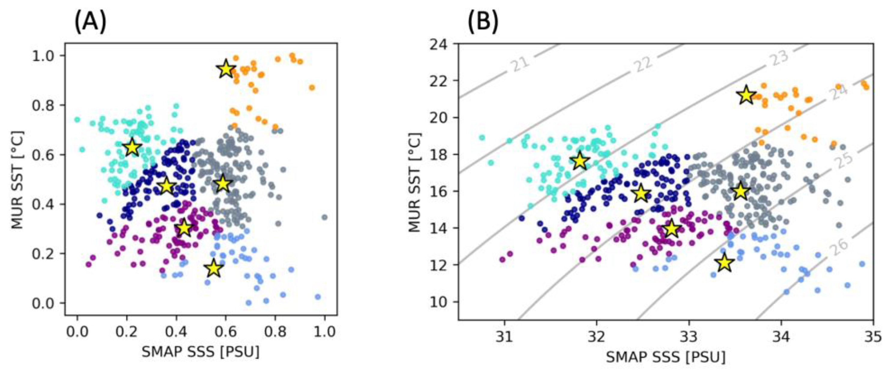
3.2.2. Uncertainty and Biases

When all the remote sensing collocated data points are considered (475), 65% of them were classified correctly (i.e., in the same cluster as the Saildrone in situ data). Most of the incorrectly classified data are located in Northern California and around the plume of the Columbia River, corresponding mostly to the clusters with transition characteristics (mid SST and mid SSS; Figure 3). When the proportion of correct/incorrect classification of data was calculated for each cluster (the total number of points based on the Saildrone in situ data), the blue cluster had the lowest proportion (43.3%) while the turquoise and orange clusters had the highest at 89.4% and 88%, respectively (Table 2).
We further investigated the source of the uncertainty by examining the differences between the SSS and SST collocated data and the Saildrone in situ data (Figure 4). The largest differences were found in coastal areas, as expected from the land contamination issue and modeling of coastal SSS data in the L3 product given its resolution [20], but this was also observed in SST. Both SST and SSS show negative differences on average between remote sensing and in situ data (−0.642 and −0.116, respectively, for the 0–50 km region), although individual large positive differences are also found in SSS in coastal areas. SST errors can be associated with its re-gridding to the lower SSS resolution.

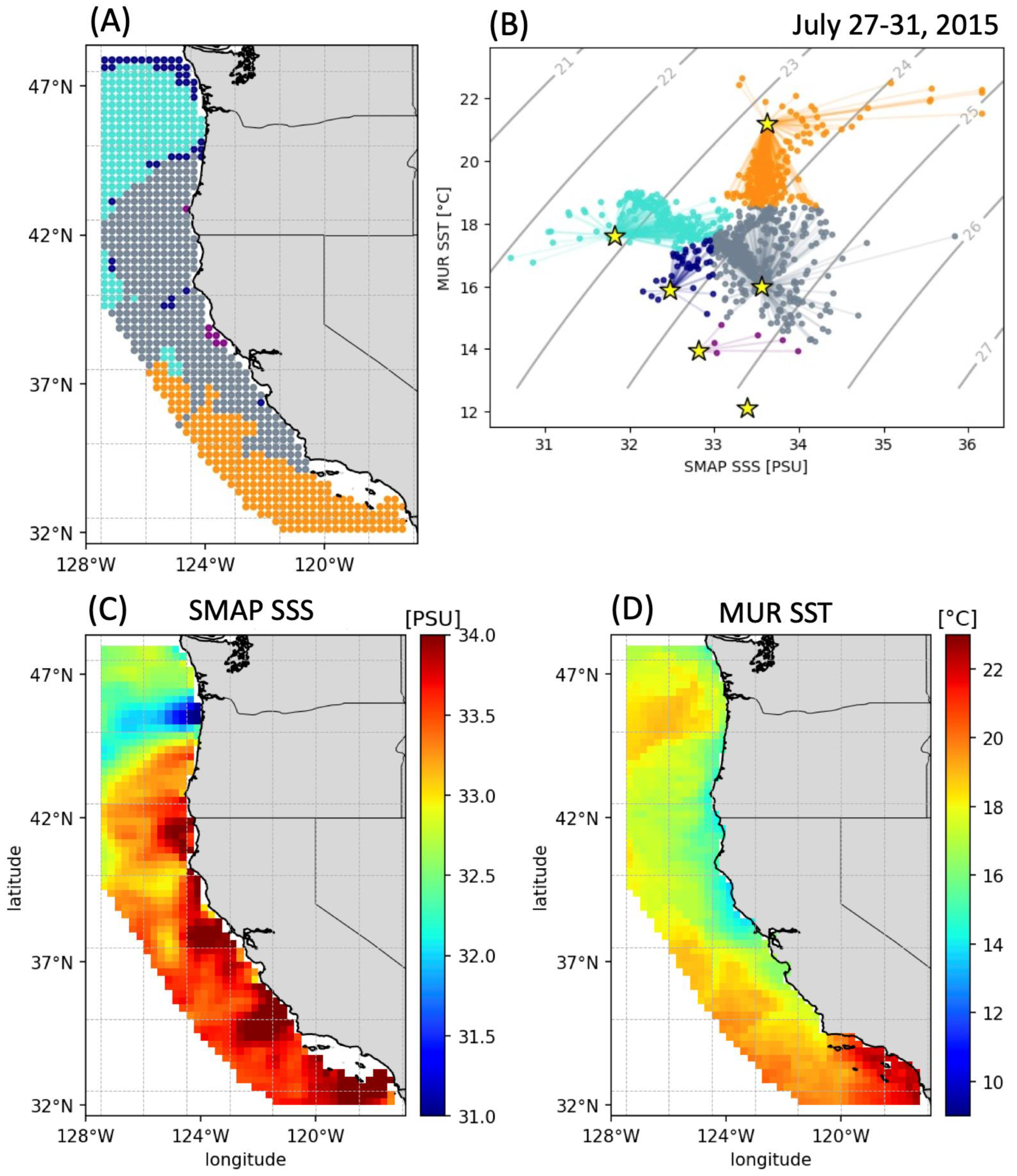
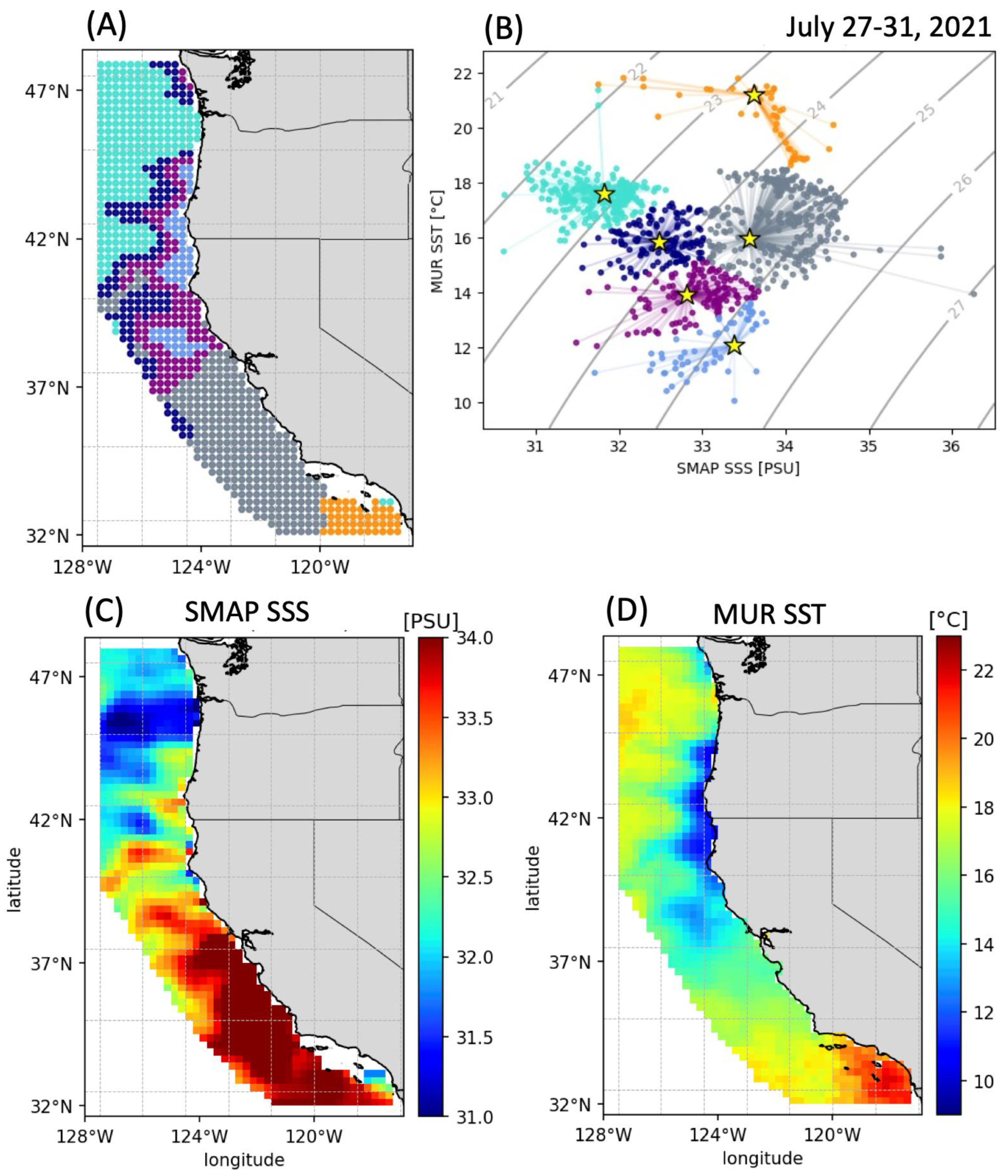
3.3. Remote Sensing Gridded Data

3.3.1. Summer Climatology

The averaged values of remote sensing gridded SST and SSS from July to September were classified, colored, and mapped according to the Saildrone in situ data centroids and are depicted in the T-S diagram in Figure 5. It is worth noting that in this classification, there are an increased number of data points offshore where Saildrone and collocated data were sparse. In the gridded data, clusters are more regionally defined on the map. The orange, gray, navy, and turquoise gridded data clusters are similarly located to those from Saildrone in situ data. The navy data has a more defined area around the turquoise water related to the Columbia River plume and offshore of the purple cluster in Northern California and Southern Oregon. The purple cluster dominates the coastal area in Central California and Southern Oregon, and only a few points of data on this map and T-S diagram correspond to the blue cluster. This is due to the short-lived nature of the cool–saline conditions associated with upwelling events that last only days to weeks and are averaged with the fast-warming conditions during the relaxation of winds during the summer [26], moving the averaged values toward classification as the purple cluster.

3.3.2. Variability in T-S Conditions

To illustrate the use of this T-S framework to describe different conditions in the CCS, we selected two periods of five days (27–31 July) for the years 2015 and 2021; remote sensing gridded data were averaged over this 5-day period before clustering. During 2015, the CCS was immersed in an extreme and extended marine heatwave (MHW) that started in 2014 and lasted until mid-2016, impacting the whole West Coast [27], while 2021 was a year considered normal in comparison [28,29]. Figure 6 and Figure 7 show the T-S diagram and cluster-colored map for each of these periods, along with the maps of SSS and SST for the same period for comparison.
During the MHW in 2015, three clusters were dominant: orange, gray, and turquoise (Figure 6A). The orange cluster extends further north and offshore, and not only in Southern California as in the climatology or the in situ data Saildrone overlapping period. The turquoise cluster waters have a similar pattern as in the climatology, although the T-S diagram shows that these data points in general have higher salinity and overall higher temperature values than the climatology and the in situ Saildrone data. The gray-colored data points are shifted further north in Northern California and Oregon, inshore and offshore, and only onshore in Central California. For this period, few purple and no blue data points are observed, showing that cool–saline water was generally absent during this period (Figure 6B), as it corresponds with the occurrence of the extreme MHW [27]. In contrast, in 2021, data belonging to all clusters are present (Figure 7A,B) in a distribution similar to the climatology and the in situ Saildrone data. At this time, a clear area of cool water is seen in Oregon and Northern California, indicating upwelling (Figure 7D), although salinity is relatively low (Figure 7B). The gray cluster in Central and offshore Central California is in this case highly saline, as seen in the SSS map (Figure 7C). Note that there are a couple of turquoise points in Southern California, but the T-S diagram (Figure 7B) shows that they are better (visually) aggregated with the orange cluster.

4. Discussion

In this paper, we present a new methodology to describe variability in surface ocean conditions using remote sensing temperature and salinity in coastal regions. While SST variability can be accurately described in coastal regions using satellite data thanks to its high spatial resolution, the lower resolution and large uncertainties of SSS near land challenge its use at the coast. Here, we combine a classic oceanographic T-S diagram framework and a data clustering technique to aggregate distinct surface water characteristics in a coastal region using in situ data. This allows us to classify remote sensing SST and SSS into these identified clusters and describe how conditions vary at the surface and at the coast.
We illustrate this methodology in the CCS during the months of July to September, using in situ surface data from an uncrewed Saildrone vessel. Our goal is to demonstrate that this method can be useful to describe variability in surface ocean conditions in coastal areas and with an ample coverage in space and time, including dynamic and coastal areas where the spatial resolution of the data allows it. Moreover, this T-S framework can be used in near-real time given the fast availability of remote sensing data, with potential to be used in management and planning.

4.1. Surface CCS Conditions Based on Saildrone In Situ Data

First, we described surface conditions along the CCS in a T-S diagram using in situ data collected by uncrewed Saildrone vessels. The T-S diagram shows water with different properties, and despite the many processes that impact surface water, data were aggregated in identifiable clusters. For the summer CCS data, Saildrone in situ data had a tilted V shape. Although surface waters have different properties than the at-depth water masses identified in the area, our T-S representation does resemble the distribution of these waters in the T-S diagram described by [3]: (i) the Pacific Subarctic Upper Water coming from the north along the California Current, starting cold and saline, and increasing its temperature while decreasing in salinity as it surfaces; (ii) the Eastern North Pacific Central Water, offshore of the CCS, but intruding into it; and (iii) the Pacific Equatorial Water flowing northward in the California Undercurrent, both cold and saline at depth, but increasing their temperature with just slightly changing salinity as they surface. In the CCS, these different water masses are not only mixed into the surface, but also brought toward the surface through Ekman transport, Ekman pumping, and topographic upwelling; therefore, water masses with conditions resembling those of deeper waters are expected. Finally, surface waters are also influenced by river runoff, with the largest impact being from the Columbia River, which has a large footprint offshore and downstream [4].
Secondly, we aggregated the Saildrone in situ data into clusters and defined their centroids, which were later used to classify the remote sensing data, reclassify the in situ data, compare the two data types, and quantify the uncertainty. The clusters in the reclassified Saildrone in situ data describe the T-S branches more clearly, and also describe distinct regions in the CCS. The T-S clustering framework divides the CCS into four general regions differently from how it is often divided based on temperature or upwelling conditions alone [14]. In the summer, surface T-S data divide the CCS into the following regions: (1) a southern region with warm and high salinity waters in the Southern California Bight; (2) a northern region, normally considered north of Cape Mendocino (~42°N), which here begins in mid-Oregon and extends offshore, corresponding to surface waters dominated by subarctic input from the east and north and the low-salinity waters associated with the Columbia River; (3) a central region with high-salinity surface water that prevails in central California and also offshore of Northern California and Southern California; finally, (4) a region of cold and saline waters at the coast in Northern California and Southern Oregon associated with coastal upwelling. These regions have been independently described in terms of near-surface temperature or salinity since the 1980s [4,30], showing increased consistency with satellite data in recent decades. Furthermore, this clustering method allows us to describe the surface water masses as a single descriptor, as with water masses at depth, that can be clearly observed in a single map.

4.2. Surface CCS Conditions Based on Remote Sensing Data

Since we have shown that the Saildrone in situ data clusters adequately represent CCS summer surface conditions, we explore how the classification of remote sensing collocated data compare to it. While the remote sensing data are more dispersed than the in situ data, the data points are still located around the centroids defined by the in situ data clusters. More importantly, the collocated data correspond to similar locations to the Saildrone data, identifying similar regions with distinct water surface properties. The southern and northern regions are clearly identified with similar boundaries, and the Central California region has a similar location, near and offshore in the area, extending to offshore Southern California and also in northern California and Southern Oregon for the remote sensing collocated data. The navy and purple clusters of collocated data occupy a similar region around data associated with the Columbia River in Oregon and Washington, but in Northern California the purple cluster appears closer to the coast than in the in situ data. In particular, the blue cluster that appears in nearshore northern California in the in situ Saildrone data is further offshore and north in the collocated data, partially due to the lack of satellite data and partially due to uncertainties and biases in the SSS data nearshore.
We then explored the use of this T-S framework using all available gridded remote sensing data for the months of July–September. The averaged values (summer climatology) showed that, apart from a few outlier values (Figure 5), the T-S diagram and the cluster-colored map identified the location of clusters similar to those from the Saildrone in situ data. Furthermore, the purple cluster is clearly limited to coastal Northern California and Southern Oregon, with only a few blue cluster points associated with coastal upwelling. The navy cluster is more clearly depicted as a transition between the turquoise and the purple and gray clusters in the map. Using gridded data has the advantage of expanding the coverage offshore, showing that the central (and even in southern California) gray cluster waters are dominant and the turquoise cluster expands offshore as well, identifying them as a mix with the California Current System waters and coastal processes; the turquoise cluster mixes also with the precursor of the CCS, the North Pacific Current waters [31].
In the climatology, few points are classified into the blue cluster, highlighting the synoptic scale of variability of the upwelling events in the Northern California and Southern Oregon region during this time of year [26]. These events bring cold and saline water to the surface, but are interspersed with periods of strong warming—when averaged though the season and years, this results in warmer and lower salinity data points classified as purple or even gray clusters. Using daily data in the climatological classification is necessary to observe the extent of the blue cluster. On the other hand, if climatological data were used in the clustering of conditions (for example, for other regions without in situ data), some short-lived events could be missed.
Fortunately, remote sensing data are available at daily scales, allowing us to see snapshots of surface water conditions at synoptic scales. In this manuscript, it is impossible to show the classification of all remote sensing data available, but we present two 5-day periods to illustrate the use of this methodology to observe changes in the ocean surface conditions over short temporal periods and with a spatial coverage not available in any other observational dataset. The 5-day period in 2021 (Figure 7) shows the data points of each of the clusters, with a large area identified into the blue cluster associated with coastal upwelling. The SST map in Figure 7D illustrates the footprint of this upwelling event as cooler temperatures, although it is not clearly visible in the SSS map (Figure 7C). Although 2021 could be classified as a more ‘normal’ year than 2015, it does contrast with the climatology in that many of the data points associated with the gray cluster have high salinity, clearly visible in the SMAP SSS map and the T-S diagram. In particular, a shift in surface water conditions seems to occur across shore ~38°N where cool waters associated with upwelling stop, increased salinity is observed, and the cluster classification changes from blue and purple to gray. This period also illustrates that some outliers in the SSS map or the T-S diagram are not so in the colored map, as they are correctly classified into the closer cluster. This demonstrates the advantage of the clustering method, which, despite uncertainties in SSS and SST, can still utilize the data to show variability in surface conditions. In this analysis, we did not remove the outliers to illustrate this point, but we also found that coastal data cannot be used in isolation and/or in a quantitative manner.
The July period in 2015 (Figure 6) shows a different picture for the surface ocean conditions than 2021. There is no deep, cool water associated with coastal upwelling, and very few purple cluster data points. This is due not to a lack of upwelling but more importantly to the high stratification caused by the extreme MHW that prevailed along the West Coast in 2014–2016 [27], preventing deep waters from reaching the surface. The colored map in Figure 6A also shows that in addition to the limited presence or absence of blue, purple, and navy cluster points, the orange cluster was extended north off Central California due to the higher SST values associated with the MHW. Interestingly, the nearshore off Central California remained relatively cool (gray cluster), although high SSS values can be seen in the SSS map and T-S diagram. During the early period of SSS data from the SMAP mission, April–August 2015, a bias in the data was reported due to the use of different rates of data collection between this period and later on [32]. This bias is corrected in the SMAP dataset V6, available now for the RSS (Remote Sensing System) SSS data product [32], but not yet for the JPL SSS data product used in this analysis. Despite this, the illustrated 2015 period shows large differences compared to other years, and this T-S framework presents the 2014–2016 MHW from a new perspective, showing aspects of the surface CCS structure that were unchanged, such as the Columbia River plume, the ‘cooler’ coastal Central California, and Southern California, but conditions were largely different in the coastal upwelling area in Northern California and offshore of Central California. The use of this T-S framework in near-real time during extreme events like the MHW could be useful to identify areas of bigger concern, not only due to high SSTs but also to other impacted air–sea–land iterations.

4.3. Uncertainty

A major challenge in the use of remote sensing data in coastal and other challenging areas are the biases and errors due to resolution, land contamination, and clouds [10], which for SSS can be large in comparison with SST. Because SSS is based on L-band microwave radiometry, errors are dominated by land contamination and spatial resolution. In addition, L3 SSS product estimates near the coast might introduce an error due to the extrapolation of larger-scale process than coastal ones [20]. In the case of the high-resolution MUR SST data, based on infrared and microwave sensors, the dominant cause of the errors is cloud contamination [16]. In coastal upwelling regions, commonly occurring clouds and fog lead to high-resolution data gaps, leaving only the lower-resolution microwave data that might not capture the upwelling-related SST gradients [33]. While in this work we are not aiming for a quantitative description of the surface characteristics of the CCS, we still need to estimate the uncertainty of the methodology and data. Away from the coast (>100 km), the data are generally highly accurate and consistent with other descriptions of CCS surface values [3,13], especially considering the dynamical nature of the CCS and of the Saildrone trajectories. However, errors or differences can be significant in some points (Figure 4), in particular for SSS where values vary in a smaller range than SST. SST differences tend to be negative (higher SST values in the remote sensing data than in situ data), which is surprising as the MUR SST, as with other L4 datasets, tends to have positive biases in upwelling areas due to the persistent presence of clouds [33]. This uncertainty could be partially attributed to the re-gridding of the MUR SST data to a lower resolution grid to match the SSS data. Overall, the largest uncertainties are limited to the coastal data points (<50 km), and these points could be removed from the data before applying the T-S framework methodology if they are identified as outliers in the T-S diagram or the map. We decided not to do so in this analysis to demonstrate the magnitude of the uncertainties and errors, and how despite this, the T-S methodology can highly accurately describe data in the CCS if we consider four main clusters and two others of transitional conditions. Furthermore, these outlier coastal points show data that are potentially erroneous and the classification makes this more evident for their removal.
The only data for which this methodology has a large uncertainty is the blue cluster, where the classification was correct less than half of the time. This cluster represents the recently upwelled water at the coast, and besides the problems of land contamination at the coast, the resolution might be inadequate to accurately describe a process that is highly dynamic and at higher spatial scales than the remote sensing data. Despite this, the occurrence of data classified into the blue cluster in July 2015 shows that the methodology is capable of identifying recently upwelled waters, but that caution should be used in interpreting coastal data from 2015 due to the instrument rate bias mentioned above. Another error source at the daily scales at which upwelling plumes could change is the smoothing and interpolation of SSS data into a daily grid (from 8-day averages) in comparison with the high resolution (daily averaged) of the Saildrone SSS. While a more accurate comparison might be made with L2 SSS products, [11] showed that these daily collocations adequately represent gradients in conditions associated with coastal upwelling. Furthermore, we aim to illustrate variability in surface T-S conditions, not necessarily the quantification of mesoscale or finer structures. However, future work focused on the upwelling (spring–summer) vs. other seasons and in a narrower area where upwelling is dominant would be needed to examine if the uncertainties are in fact due to a resolution issue with the re-gridded MUR SST data, as it does not resolve the highest spatial scales associated with upwelling events, or are related to the larger SSS data coastal errors.
This methodology can easily be expanded to other seasons within this region and to other regions as well. Ideally, some in situ observations would be available to perform the clustering, as shown in this work. Even if in situ data are not available, the climatology analysis showed that remote sensing data can capture most clusters that the in situ data also capture, except the cluster representing short-lived conditions. The clustering analysis can then be performed on a random subset of the satellite data. For the CCS, this approach can be used to describe surface T-S conditions in other seasons when no Saildrone data are available. To facilitate the analysis, separating the data by seasons would avoid a T-S diagram with overlapping patterns that would complicate the clustering process, as different seasonal processes occur through the year (for example, precipitation in the winter and strong seasonal heating in the summer). In other regions, a preliminary inspection of the seasonality of the data would be necessary.

5. Conclusions

In this work, we demonstrated that the clustering T-S framework can be useful in describing surface temperature and salinity conditions in the coastal ocean. Describing the data using separated clusters with particular conditions, as commonly performed with water masses at depth, reduces the uncertainty in remote sensing coastal data, expanding the use of SSS. We present here the specific case of the CCS, where previous studies and in situ data are available, to assess the validity and accuracy of the method. However, this method can be expanded to other regions with or without in situ data to train the clustering. As shown here, this T-S framework (or in this case SST-SSS framework) identifies regions beyond those identified only by SST and that reflect processes and air–sea–land interactions that further describe the surface ocean dynamics. Furthermore, this methodology takes advantage of the SSS dataset, a vast and growing source of global data, which is still underutilized in coastal areas. Our results provide a potential breakthrough for the application of SSS in coastal regions where connections to biological productivity are crucial.

Author Contributions

Conceptualization, M.G.-R.; methodology, M.G.-R. and G.K.; formal analysis, G.K.; investigation, M.G.-R. and J.V.-C.; writing—original draft preparation, M.G.-R. and G.K.; writing—review and editing, M.G.-R., G.K. and J.V.-C. All authors have read and agreed to the published version of the manuscript.

Funding

This research was funded by the National Aeronautics and Space Administration (NASA): grant numbers 80NSSC20K0768, 80NSSC20K1003 NASA.

Data Availability Statement

Remote sensing data is publicly available at https://podaac.jpl.nasa.gov/, and Saildrone in situ data from https://www.saildrone.com/. Saildrone data used in this analysis can be accessed directly through https://data.saildrone.com/id/2089, accessed 1 November 2023 and https://data.saildrone.com/id/2120, accessed 1 November 2023, MUR SST data may be accessed directly through https://podaac.jpl.nasa.gov/dataset/MUR-JPL-L4-GLOB-v4.1, accessed 1 November 2023 and SMAP data may be accessed directly through https://podaac.jpl.nasa.gov/dataset/SMAP_JPL_L3_SSS_CAP_8DAY-RUNNINGMEAN_V5, accessed 1 November 2023. The collocated data used in this analysis is available upon request. The scripts to perform the analysis and figures are available at https://github.com/farallon-institute/Garcia-Reyes_etal_2024_SaildroneTS, accessed 1 November 2023.

Acknowledgments

Thank you to the NOAA, Fisheries and Oceans Canada (DFO), and Saildrone for collecting and providing the in situ data for this analysis. Thanks to Chelle Gentemann for performing the collocation of the satellite data to the Saildrone data and also to Sarah Ann Thompson for editing of the manuscript.

Conflicts of Interest

The authors declare no conflicts of interest.

Appendix A

Figure A1. T-S diagrams of remote sensing collocated Satellite data, colored by cluster based on Saildrone in situ data. (A) Normalized SST and SSS values over which the nearest centroid is calculated; (B) T-S diagram with denormalized values after clustering.
Remotesensing 16 01311 g0a1

References

  1. Vinogradova, N.; Lee, T.; Boutin, J.; Drushka, K.; Fournier, S.; Sabia, R.; Stammer, D.; Bayler, E.; Reul, N.; Gordon, A.; et al. Satellite salinity observing system: Recent discoveries and the way forward. Front. Mar. Sci. 2019, 6, 428925. [Google Scholar] [CrossRef]
  2. Tomczak, M., Jr. A multi-parameter extension of temperature/salinity diagram techniques for the analysis of non-isopycnal mixing. Prog. Oceanogr. 1981, 10, 147–171. [Google Scholar] [CrossRef]
  3. Bograd, S.J.; Schroeder, I.D.; Jacox, M.G. A water mass history of the Southern California current system. Geophys. Res. Lett. 2019, 46, 6690–6698. [Google Scholar] [CrossRef]
  4. Huyer, A. Coastal upwelling in the California Current system. Prog. Oceanogr. 1983, 12, 259–284. [Google Scholar] [CrossRef]
  5. Minnett, P.; Alvera-Azcárate, A.; Chin, T.; Corlett, G.; Gentemann, C.; Karagali, I.; Li, X.; Marsouin, A.; Marullo, S.; Maturi, E.; et al. Half a century of satellite remote sensing of sea-surface temperature. Remote Sens. Environ. 2019, 233, 111366. [Google Scholar] [CrossRef]
  6. Chelton, D.B.; Esbensen, S.K.; Schlax, M.G.; Thum, N.; Freilich, M.H.; Wentz, F.J.; Gentemann, C.L.; Mcphaden, M.J.; Schopf, P.S. Observations of coupling between surface wind stress and sea surface temperature in the eastern Tropical Pacific. J. Clim. 2001, 14, 1479–1498. [Google Scholar] [CrossRef]
  7. Reul, N.; Tenerelli, J.; Chapron, B.; Vandemark, D.; Quilfen, Y.; Kerr, Y. SMOS satellite L-band radiometer: A new capability for ocean surface remote sensing in hurricanes. J. Geophys. Res. Ocean. 2012, 117, 7474. [Google Scholar] [CrossRef]
  8. Lagerloef, G.; deCharon, A.; Lindstrom, E. Ocean salinity and the Aquarius/SAC-D mission: A new frontier in ocean remote sensing. Mar. Technol. Soc. J. 2013, 47, 26–30. [Google Scholar] [CrossRef]
  9. Entekhabi, D.; Yueh, S.; O’neill, P.; Kellogg, K.; Allen, A.; Bindlish, R.; Brown, M.E.; Chan, S.; Colliander, A.; Crow, W.; et al. SMAP Handbook Soil Moisture Active Passive: Mapping Soil Moisture and Freeze/Thaw from Space; JPL CL14-2285; Jet Propulsion Laboratory: Pasadena, CA, USA, 2014. [Google Scholar]
  10. Tang, W.; Yueh, S.H.; Fore, A.G.; Vazquez-Cuervo, J.; Gentemann, C.; Hayashi, A.K.; Akins, A.; García-Reyes, M. Using Saildrones to Assess the SMAP Sea Surface Salinity Retrieval in the Coastal Regions. IEEE J. Sel. Top. Appl. Earth Obs. Remote Sens. 2022, 15, 7042–7051. [Google Scholar] [CrossRef]
  11. Vazquez-Cuervo, J.; García-Reyes, M.; Gómez-Valdés, J. Identification of Sea Surface Temperature and Sea Surface Salinity Fronts along the California Coast: Application Using Saildrone and Satellite Derived Products. Remote Sens. 2023, 15, 484. [Google Scholar] [CrossRef]
  12. Sabia, R.; Ballabrera, J.; Lagerloef, G.; Bayler, E.; Talone, M.; Chao, Y.; Donlon, C.; Fernandez-Prieto, D.; Font, J. Derivation of an experimental satellite-based TS diagram. In Proceedings of the 2012 IEEE International Geoscience and Remote Sensing Symposium, Munich, Germany, 22–27 July 2012; pp. 5760–5763. [Google Scholar] [CrossRef]
  13. Sabia, R.; Klockmann, M.; Fernández-Prieto, D.; Donlon, C. A first estimation of SMOS-based ocean surface T-S diagrams. J. Geophys. Res. Ocean. 2014, 119, 7357–7371. [Google Scholar] [CrossRef]
  14. Checkley, D.M., Jr.; Barth, J.A. Patterns and processes in the California Current System. Prog. Oceanogr. 2009, 83, 49–64. [Google Scholar] [CrossRef]
  15. Gentemann, C.L.; Scott, J.P.; Mazzini, P.L.F.; Pianca, C.; Akella, S.; Minnett, P.J.; Cornillon, P.; Fox-Kemper, B.; Cetinić, I.; Chin, T.M.; et al. Saildrone: Adaptively sampling the marine environment. Bull. Am. Meteorol. Soc. 2020, 101, E744–E762. [Google Scholar] [CrossRef]
  16. Chin, T.M.; Vazquez-Cuervo, J.; Armstrong, E.M. A multi-scale high-resolution analysis of global sea surface temperature. Remote Sens. Environ. 2017, 200, 154–169. [Google Scholar] [CrossRef]
  17. JPL MUR MEaSUREs Project. 2015. GHRSST Level 4 MUR Global Foundation Sea Surface Temperature Analysis. Ver. 4.1. PO.DAAC, CA, USA. Available online: https://podaac.jpl.nasa.gov/dataset/MUR-JPL-L4-GLOB-v4.1 (accessed on 1 November 2023).
  18. Meissner, T.; Wentz, F.J.; Le Vine, D.M. The salinity retrieval algorithms for the NASA Aquarius version 5 and SMAP version 3 releases. Remote Sens. 2018, 10, 1121. [Google Scholar] [CrossRef]
  19. Fore, A.G.; Yueh, S.H.; Tang, W.; Stiles, B.W.; Hayashi, A.K. Combined Active/Passive Retrievals of Ocean Vector Wind and Sea Surface Salinity with SMAP. IEEE Trans. Geosci. Remote Sens. 2016, 54, 7396–7404. [Google Scholar] [CrossRef]
  20. Fore, A.; Yueh, S.; Tang, W.; Hayashi, A. SMAP Salinity and Wind Speed Data User’s Guide; California Institute of Technology: Pasadena, CA, USA, 2020; p. 42. [Google Scholar]
  21. Hall, K.; Daley, A.; Whitehall, S.; Sandiford, S.; Gentemann, C.L. Validating Salinity from SMAP and HYCOM Data with Saildrone Data during EUREC4A-OA/ATOMIC. Remote Sens. 2022, 14, 3375. [Google Scholar] [CrossRef]
  22. Hoyer, S.; Hamman, J. xarray: N-D labeled Arrays and Datasets in Python. J. Open Res. Softw. 2017, 5, 10. [Google Scholar] [CrossRef]
  23. Maze, G.; Mercier, H.; Fablet, R.; Tandeo, P.; Radcenco, M.L.; Lenca, P.; Feucher, C.; Le Goff, C. Coherent heat patterns revealed by unsupervised classification of Argo temperature profiles in the North Atlantic Ocean. Prog. Oceanogr. 2017, 151, 275–292. [Google Scholar] [CrossRef]
  24. Jones, D.C.; Holt, H.J.; Meijers, A.J.S.; Shuckburgh, E.F. Unsupervised clustering of Southern Ocean Argo float temperature profiles. J. Geophys. Res. Ocean. 2019, 124, 390–402. [Google Scholar] [CrossRef]
  25. Pedregosa, F.; Varoquaux, G.; Gramfort, A.; Michel, V.; Thirion, B.; Grisel, O.; Blondel, M.; Müller, A.; Nothman, J.; Louppe, G.; et al. Scikit-learn: Machine learning in Python. J. Mach. Learn. Res. 2011, 12, 2825–2830. [Google Scholar]
  26. García-Reyes, M.; Largier, J.L. Seasonality of coastal upwelling off central and northern California: New insights, including temporal and spatial variability. J. Geophys. Res. Ocean. 2012, 117, 7629. [Google Scholar] [CrossRef]
  27. Gentemann, C.L.; Fewings, M.R.; García-Reyes, M. Satellite sea surface temperatures along the West Coast of the United States during the 2014–2016 northeast Pacific marine heat wave. Geophys. Res. Lett. 2017, 44, 312–319. [Google Scholar] [CrossRef]
  28. García-Reyes, M.; Sydeman, W.J. California Multivariate Ocean Climate Indicator (MOCI) [Data set, V2]. Farallon Institute Website. 2017. Available online: http://www.faralloninstitute.org/moci (accessed on 1 May 2023).
  29. Thompson, A.R.; Bjorkstedt, E.P.; Bograd, S.J.; Fisher, J.L.; Hazen, E.L.; Leising, A.; Santora, J.A.; Satterthwaite, E.V.; Sydeman, W.J.; Alksne, M.; et al. State of the California Current Ecosystem in 2021: Winter is coming? Front. Mar. Sci. 2022, 9, 958727. [Google Scholar] [CrossRef]
  30. Lynn, R.J.; Simpson, J.J. The California Current System: The seasonal variability of its physical characteristics. J. Geophys. Res. Ocean. 1987, 92, 12947–12966. [Google Scholar] [CrossRef]
  31. Hristova, H.G.; Ladd, C.; Stabeno, P.J. Variability and trends of the Alaska Gyre from Argo and satellite altimetry. J. Geophys. Res. Ocean. 2019, 124, 5870–5887. [Google Scholar] [CrossRef]
  32. Meissner, T.; Wentz, F.; Manaster, A.; Lindsley, R.; Brewer, M.; Densberger, M. NASA/RSS SMAP Salinity: Version 6.0 Validated Release. RSS Tech. Rep. 2024, 01182. [Google Scholar]
  33. Meneghesso, C.; Seabra, R.; Broitman, B.R.; Wethey, D.S.; Burrows, M.T.; Chan, B.K.; Guy-Haim, T.; Ribeiro, P.A.; Rilov, G.; Santos, A.M.; et al. Remotely-sensed L4 SST underestimates the thermal fingerprint of coastal upwelling. Remote Sens. Environ. 2020, 237, 111588. [Google Scholar] [CrossRef]
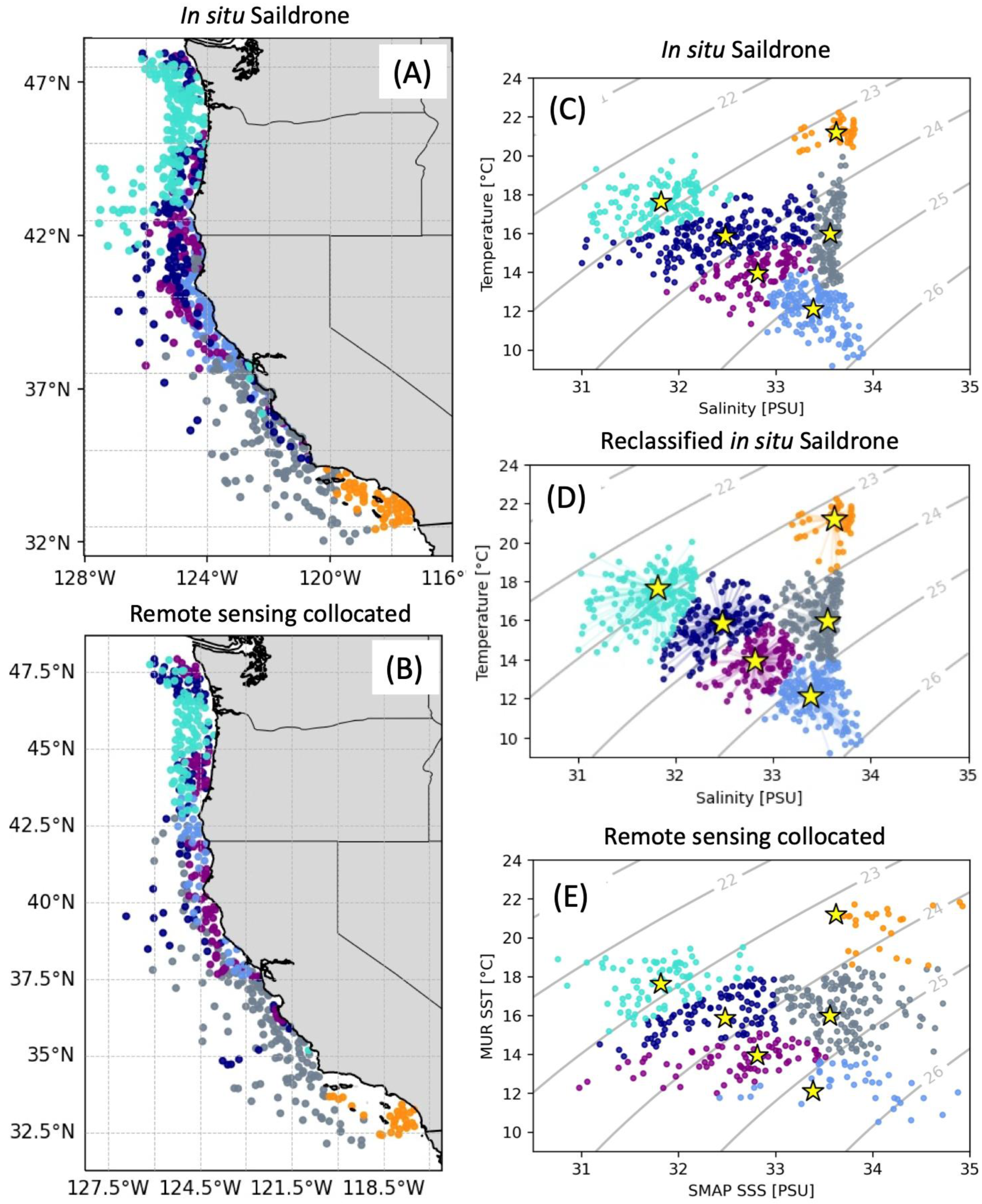
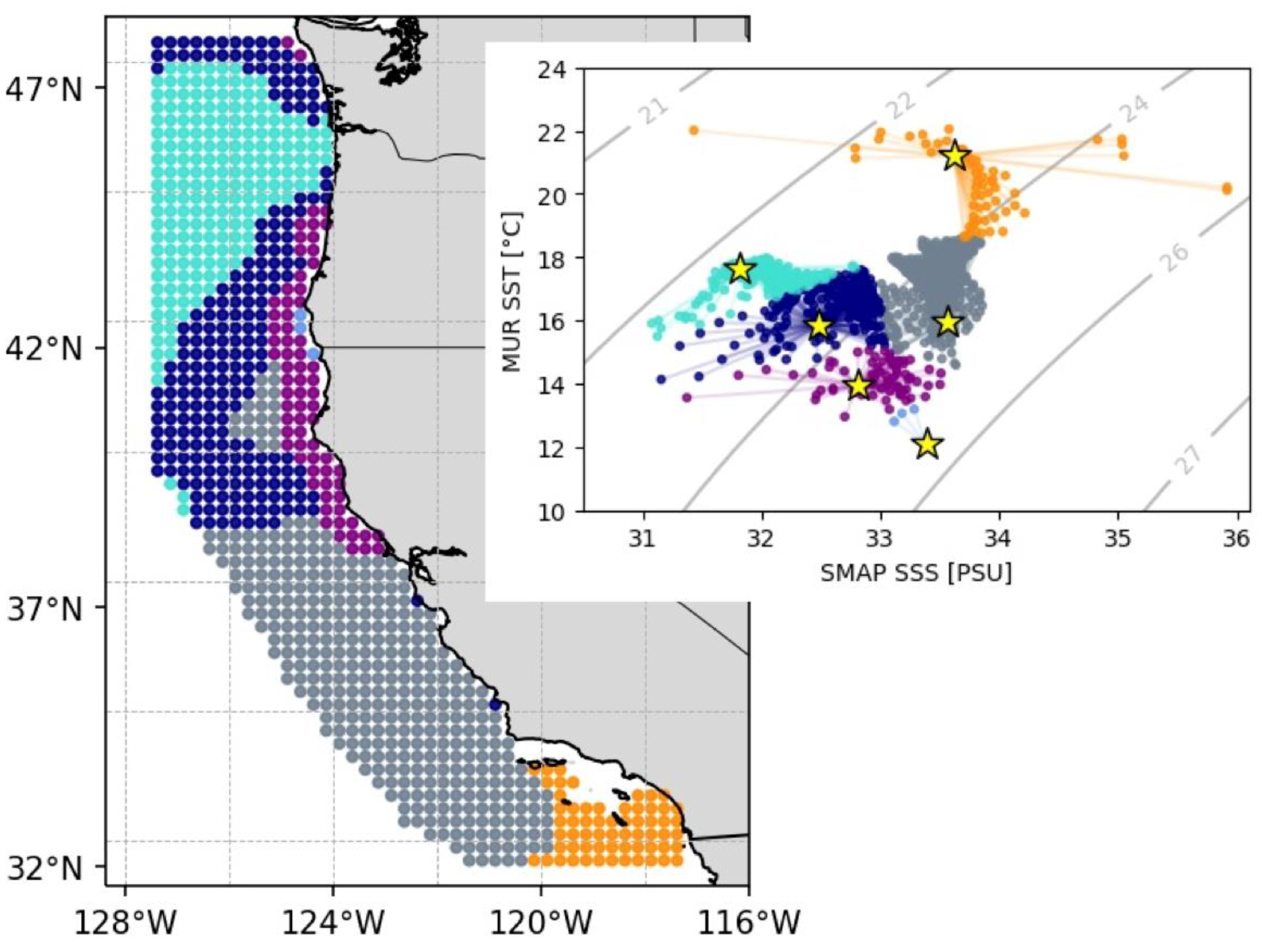
Figure 1. Saildrone in situ data aggregated daily, displayed by location (left) and day of year vs. latitude (right). Data period: July–September 2018 (red) and 2019 (blue).
Remotesensing 16 01311 g001
Figure 2. (A) Mapping of reclassified Saildrone in situ data colored by clustering in (D). (B) Mapping of remote sensing collocated data colored by clustering shown in (E). (C) T-S diagram Saildrone in situ data, colored by the clustering analysis. (D) Saildrone in situ data reclassified using the closest centroid method. (E) Classification of remote sensing collocated data based on centroids from Saildrone in situ data shown in (C). Yellow stars indicate cluster centroids.
Remotesensing 16 01311 g002
Figure 3. Proportion of correct vs. incorrect classified remote sensing collocated data by cluster defined by Saildrone in situ data centroids. (A) Location of the correctly/incorrectly classified data. (B) T-S plot showing the collocated data. Green points are the correctly classified data; red points are the incorrectly classified data.
Remotesensing 16 01311 g003
Figure 4. Differences in SSS and SST between the remote sensing collocated data and the Saildrone in situ data, plotted as bimodal density distributions. (AC) show, in darker color, where the largest density of differences in salinity (x-axis) and temperature (y-axis) occur; univariate histograms show on each axis. Data are separated and colored by distance to shore: (A) 0–50 km in blue, (B) 51–100 km in orange, (C) >101 km in green, and (D) all data combined, by data points rather than densities, and probability distribution in the axis rather than histograms.
Remotesensing 16 01311 g004
Figure 5. T-S diagram and map of remote sensing gridded data averaged values for July to September from 2015 to 2023. Data are colored by clusters and centroids based on Saildrone in situ data are depicted with yellow stars.
Remotesensing 16 01311 g005
Figure 6. Map (A) and T-S diagram (B) of gridded remote sensing data for mean values of SSS in (C) and SST (D) for the period 27–31 July 2015. Cluster classification was performed based on centroid (yellow stars) from Saildrone in situ data.
Remotesensing 16 01311 g006
Figure 7. Map (A) and T-S diagram (B) of gridded remote sensing data for mean values of SSS in (C) and SST (D) for the period 27–31 July 2021. Cluster classification was performed based on centroid (yellow stars) from Saildrone in situ data.
Remotesensing 16 01311 g007
Table 1. Description of characteristics and region of each cluster based on the reclassified Saildrone in situ T-S data.
Cluster ColorCharacteristicsRegion
1—OrangeHigh SSS, High SSTSouthern California Bight
2—GrayHigh SSS, Mid SSTCentral California
3—BlueHigh SSS, Low SSTNorthern California and Southern Oregon; coastal, associated with coastal upwelling
4—PurpleMid SSS, Mid/Low SSTMostly along northern CCS and offshore of blue waters
5—NavyLow SSS, Mid SSTMostly along northern CCS, between coastal upwelling waters and Columbia River waters
6—TurquoiseLow SSS, High SSTColumbia River water mixed with northern CCS, and its extended plume offshore and south
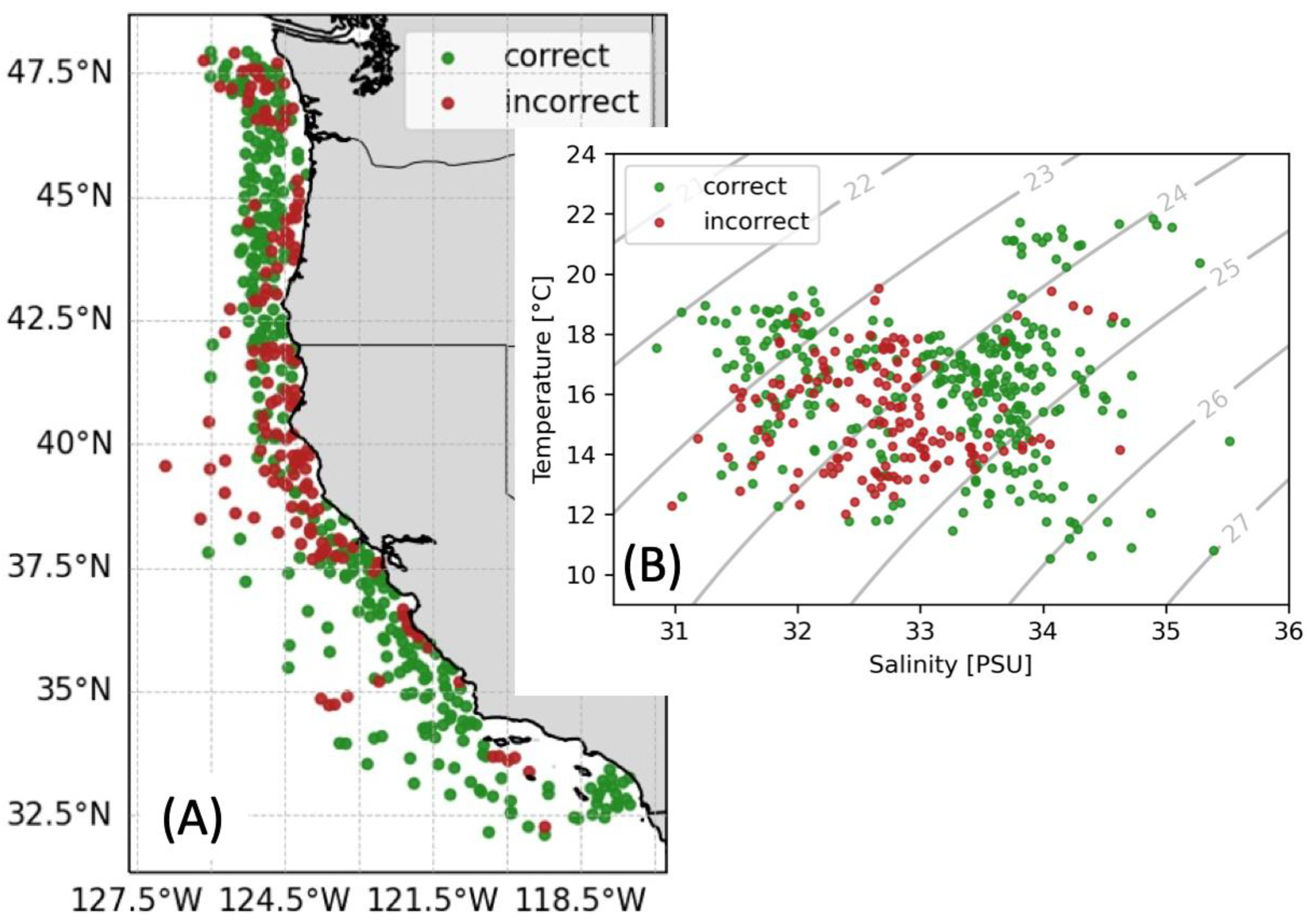
Table 2. Proportion of correct vs. incorrect classified remote sensing collocated data by cluster defined by Saildrone in situ data, expressed as percentage.
Cluster ColorOrangeGrayBluePurpleNavyTurquoise
Proportion (%)88.069.343.369.669.289.4
Disclaimer/Publisher’s Note: The statements, opinions and data contained in all publications are solely those of the individual author(s) and contributor(s) and not of MDPI and/or the editor(s). MDPI and/or the editor(s) disclaim responsibility for any injury to people or property resulting from any ideas, methods, instructions or products referred to in the content.

