

Rock Layer Classification and Identification in Ground-Penetrating Radar via Machine Learning


1
Key Laboratory of Safety Control of Bridge Engineering, Ministry of Education, Changsha University of Science & Technology, Changsha 410114, China
2
School of Civil Engineering, Changsha University of Science & Technology, Changsha 410114, China
3
State Key Laboratory of Geomechanics and Geotechnical Engineering, Institute of Rock and Soil Mechanics, Chinese Academy of Sciences, Wuhan 430071, China
*
Author to whom correspondence should be addressed.
Remote Sens. 2024, 16(8), 1310; https://doi.org/10.3390/rs16081310
Submission received: 7 February 2024
/
Revised: 23 March 2024
/
Accepted: 24 March 2024
/
Published: 9 April 2024
(This article belongs to the Topic Recent Advances in Structural Health Monitoring, 2nd Volume)
Abstract
:Ground-penetrating radar (GPR) faces complex challenges in identifying underground rock formations and lithological structures. The diversity, intricate shapes, and electromagnetic properties of subsurface rock formations make their accurate detection difficult. Additionally, the heterogeneity of subsurface media, signal scattering, and non-linear propagation effects contribute to the complexity of signal interpretation. To address these challenges, this study fully considers the unique advantages of convolutional neural networks (CNNs) in accurately identifying underground rock formations and lithological structures, particularly their powerful feature extraction capabilities. Deep learning models possess the ability to automatically extract complex signal features from radar data, while also demonstrating excellent generalization performance, enabling them to handle data from various geological conditions. Moreover, deep learning can efficiently process large-scale data, thereby improving the accuracy and efficiency of identification. In our research, we utilized deep neural networks to process GPR signals, using radar images as inputs and generating structure-related information associated with rock formations and lithological structures as outputs. Through training and learning, we successfully established an effective mapping relationship between radar images and lithological label signals. The results from synthetic data indicate a rock block identification success rate exceeding 88%, with a satisfactory continuity identification of lithological structures. Transferring the network to measured data, the trained model exhibits excellent performance in predicting data collected from the field, further enhancing the geological interpretation and analysis. Therefore, through the results obtained from synthetic and measured data, we can demonstrate the effectiveness and feasibility of this research method.
1. Introduction
Ground-penetrating radar (GPR) is a crucial geophysical exploration technique used for the non-invasive acquisition of subsurface structural and geological information. Its development history can be traced back to the early 20th century, encompassing centuries of evolution and innovation [1,2]. The fundamental principle of GPR technology involves transmitting electromagnetic waves into the ground and subsequently receiving reflected signals, thereby revealing the properties and distribution of subsurface materials. Over the past few decades, GPR has evolved into a pivotal tool in various fields, including underground exploration, soil engineering, mineral resource development, environmental science, archaeological research, and geological hazard monitoring [3,4,5].
In its initial stages, GPR primarily found applications in the military sector, where it was employed for detecting underground tunnels and landmines [6]. However, with advancements in technology and an expanding scope of utility, GPR has found widespread use in civilian sectors as well. Notably, it has been employed in groundwater exploration, soil surveys, environmental monitoring, archaeological research, and geological hazard prediction [7]. GPR contributes significantly to the determination of groundwater levels, soil layers, and rock formations, thus facilitating infrastructure planning and land utilization. Additionally, GPR plays a vital role in archaeological research by enabling non-destructive surveys of ancient sites and cultural heritage, thereby contributing to cultural preservation and historical studies [8].
Another critical application domain is geological exploration and resource development. GPR assists in identifying underground rock types, distribution, and thickness, which are crucial factors in resource development and reserve estimation [9,10,11,12]. In mineral resource exploration, GPR aids prospectors in locating underground areas with mineral potential, enhancing exploration efficiency and accuracy. Geological hazard early warning is yet another crucial field where GPR is employed, used to monitor signs of geological disasters such as landslides, earthquakes, and mudslides, enabling early warnings and mitigation of disaster risks. In civil engineering, GPR is utilized to identify underground pipelines, obstacles, and facilities, ensuring construction safety and efficiency. Over the recent decades, GPR technology has witnessed significant development, with advancements in sensors and data processing techniques enabling the acquisition of higher-resolution subsurface images, thus enhancing signal quality and usability [13,14,15,16].
The identification of geological strata plays a pivotal role in both civil engineering and geological exploration. Understanding the characteristics, distribution, and variations of subsurface layers not only facilitates infrastructure development planning but also enables the efficient extraction of underground resources and the monitoring of hydrological conditions [17]. Accurate knowledge of subsurface strata is particularly critical in managing water resources, especially in arid regions. GPR technology, with its ability to generate high-resolution subsurface images, offers valuable insights for geological engineering. It can discern interfaces, thicknesses, and characteristics of underground strata, thereby assisting engineers in assessing soil stability and bearing capacity. This information is of paramount importance in the design and construction of infrastructure projects like roads, bridges, dams, and buildings [18,19]. Additionally, GPR can be deployed to locate underground pipelines and cables, preventing damage to crucial facilities during construction and ensuring the smooth progress of projects.
Furthermore, rock-socketed steel casings are commonly employed structures in underground engineering, encompassing underground pipelines, tunnels, bridge foundations, and more. Grasping the condition and integrity of these casings is imperative for engineering safety. GPR technology not only determines the position, dimensions, and material of rock-socketed steel casings but also detects defects such as corrosion and cracks [20]. Regular GPR inspections empower engineers to proactively identify potential issues and implement appropriate maintenance and repair measures, ensuring the reliability and durability of underground structures. Additionally, GPR technology plays a significant role in environmental monitoring and geological disaster early warning systems. By monitoring changes in groundwater levels, soil moisture, and geological structures, GPR contributes to predicting the risk of geological disasters such as landslides, earthquakes, and mudslides [21]. Taking timely measures can mitigate potential impacts, safeguarding lives and property. In summary, GPR technology offers a wide range of applications in the identification of geological strata, detection of rock-socketed steel casings, and environmental monitoring and geological disaster early warning. It not only provides invaluable subsurface information but also serves as a powerful tool in various engineering projects and scientific research endeavors. This contributes to the safer and more efficient utilization of underground spaces while reducing potential risks [22].
In the field of GPR signal processing, the development of deep learning has witnessed remarkable progress [23]. With the emergence of deep neural networks, GPR signal processing has become significantly more precise and efficient. This trend has already had a significant impact in various domains, including subsurface exploration, geological engineering, and environmental monitoring [24]. Deep learning models can automatically extract complex underground signal features, eliminating the need for labor-intensive manual feature engineering. This not only accelerates signal processing but also enhances accuracy. Deep learning’s applications in GPR encompass underground target detection, stratigraphic identification, and rock formation feature analyses, among others [25]. Moreover, deep learning’s ability to handle large-scale data is crucial in subsurface exploration, where a substantial volume of radar images and signal data often requires processing. The robust computational power and generalization capabilities of deep learning models enable them to address challenges posed by different geological conditions and complex subsurface environments. Additionally, deep learning has opened up new possibilities for GPR signal processing, including multimodal data fusion, real-time monitoring, and automated analyses. These innovations are poised to further enhance our ability to acquire and interpret subsurface information, providing invaluable support for geological exploration and engineering projects [26].
Deep learning offers significant advantages in handling GPR data. Its automatic feature extraction capability eliminates the need for the manual extraction of complex underground signal features, thus enhancing processing efficiency [27]. The robust generalization ability of deep learning models enables them to adapt to data from different geological conditions, improving the versatility of data processing. Furthermore, deep learning can handle large-scale data, speeding up the analysis process and increasing identification accuracy. In this paper, we have employed advanced deep learning techniques to harness GPR data for the identification of underground rock layers and geological strata, fully capitalizing on the remarkable capabilities of this technology [28]. We have utilized convolutional neural networks (CNNs), a powerful tool in this context, to accurately extract information pertaining to rock layers and strata through the analysis and processing of GPR images. Furthermore, through the learning and training of deep neural networks, we have extended our capability to predict the composition and distribution of subsurface structures [29,30]. To better achieve our objectives, we have constructed a sophisticated UNet network architecture, incorporating multiple layers of CNNs. This architecture allows us to learn the features and spatial layout of underground structures from GPR data at various scales. Additionally, we have applied various mathematical techniques, including random media modeling, strata modeling, and time-domain finite difference methods, to construct datasets that closely mimic real-world conditions. The application of these techniques has resulted in a more accurate and reliable deep learning model [31,32,33].
In this paper, we utilize deep learning techniques for extracting information from radar data. The core idea is to use convolutional neural networks to identify hyperbolic and co-phase axis signals in radar data and output them as block and stratum information. To achieve this goal, the first part details the generation of data samples, including creating 1000 datasets, each containing a radar image and rock layer structure label. Radar images are generated using the Finite-Difference Time-Domain (FDTD) method, while rock layer labels are based on boundary information from the dielectric constant model. The random generation and distribution of strata and blocks are also discussed in this section. The second part covers the construction of the deep network model, with 80% of the sample set used as input data, including radar images and rock layer structure information, for training the deep network on a large dataset. Parameter adjustments and optimization of the network using the Adam algorithm are also conducted. The third part describes using the trained network to predict the remaining 20% of the sample data and compare it with the ground truth. Finally, the last part introduces experiments using real measured data to analyze the network’s recognition capability.
2. Materials and Methods
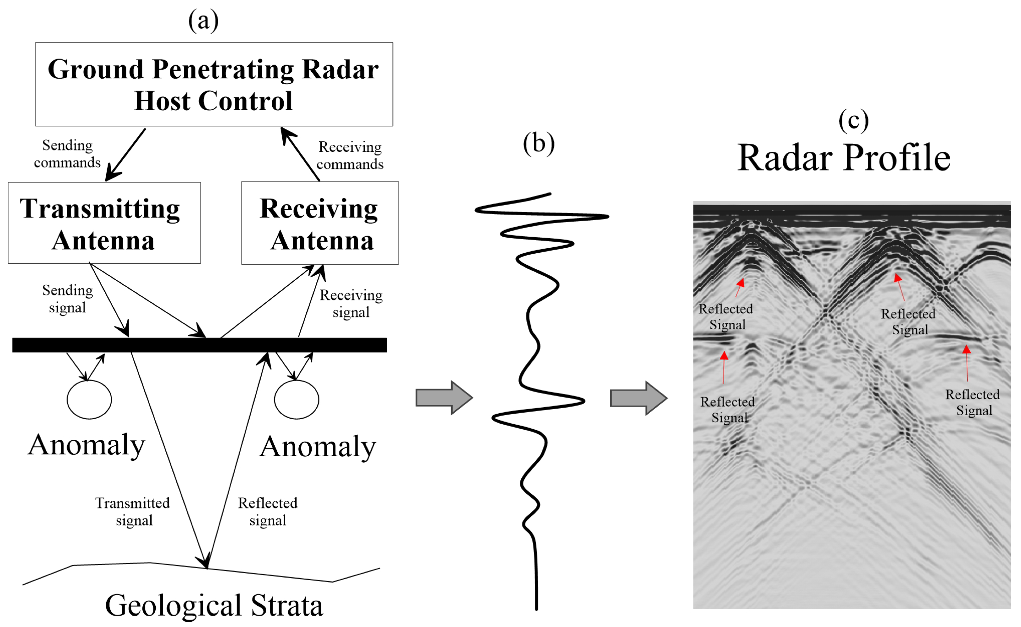
GPR uses electromagnetic waves to explore underground rock formations and stratigraphic interfaces. Initially, the radar emits high-frequency waves that interact with subsurface layers [34]. The transmission antenna projects these waves into the subterranean environment, while the receiving antenna captures and records the reflected signals. As electromagnetic waves move underground, they interact with various subsurface materials like rocks, soils, and stratigraphic interfaces, as shown in Figure 1. Some waves reflect partially, creating bright spots, while others penetrate deeper layers. These bright spots’ positions and intensities offer crucial insights into underground rock formations and stratigraphic interfaces [35].
The resulting B-scan images from GPR depict horizontal cross-sections of the underground. These images show reflection intensity and time-delay data from different depths. They mainly capture reflections from diverse subsurface materials like rocks, soils, and stratigraphic interfaces. Notably, reflections become more prominent when waves encounter layers with different dielectric constants [36]. Rock layers often show clear reflections, while soil layers may have varied reflection patterns based on material properties, density, moisture content, and wave frequency underground.
These distinctive features hold significance for geologists and engineers alike, as they facilitate the delineation of underground structures and the discernment of rock layer distributions. The comprehensive utilization of GPR technology empowers a more meticulous investigation and characterization of the attributes and spatial distribution of underground rock formations and stratigraphic interfaces [37].
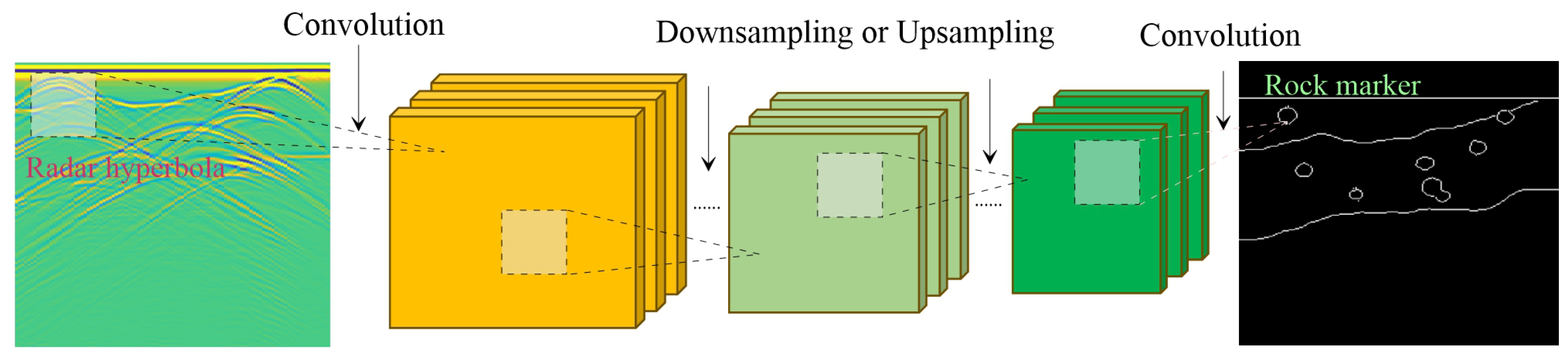
A convolutional neural network (CNN) is a specialized deep learning model tailored for image processing tasks. It excels in extracting features from input images and translating them into output images, a process essential for converting GPR B-scan images into rock structure label images, as shown in Figure 2 [24].
Initially, the CNN is fed with the GPR B-scan image containing data on underground reflection intensity and time delays. The first layer, typically a convolutional layer, employs convolutional operations using kernels to capture local features like edges and textures [38].
Subsequently, the CNN progresses through multiple convolutional and pooling layers to extract increasingly complex features from the image. Convolutional layers identify intricate image structures, while pooling layers reduce image dimensions, preserving essential information and minimizing computational complexity.
In deeper CNN layers, fully connected layers follow the final convolutional layer, transforming image features into a vector form. This vector undergoes non-linear transformations through activation functions, enhancing feature extraction.
The CNN’s output layer is customized to match the desired output, such as rock structure label images, possibly containing multiple neurons representing various label categories. Training employs backpropagation algorithms to adjust network parameters, minimizing differences between predicted and actual images.
In essence, a convolutional neural network operates through hierarchical convolution and pooling operations, extracting features from GPR B-scan images and mapping them onto rock structure label images. This automated approach greatly aids in identifying underground rock structures, serving as a valuable tool for geological research and engineering planning.
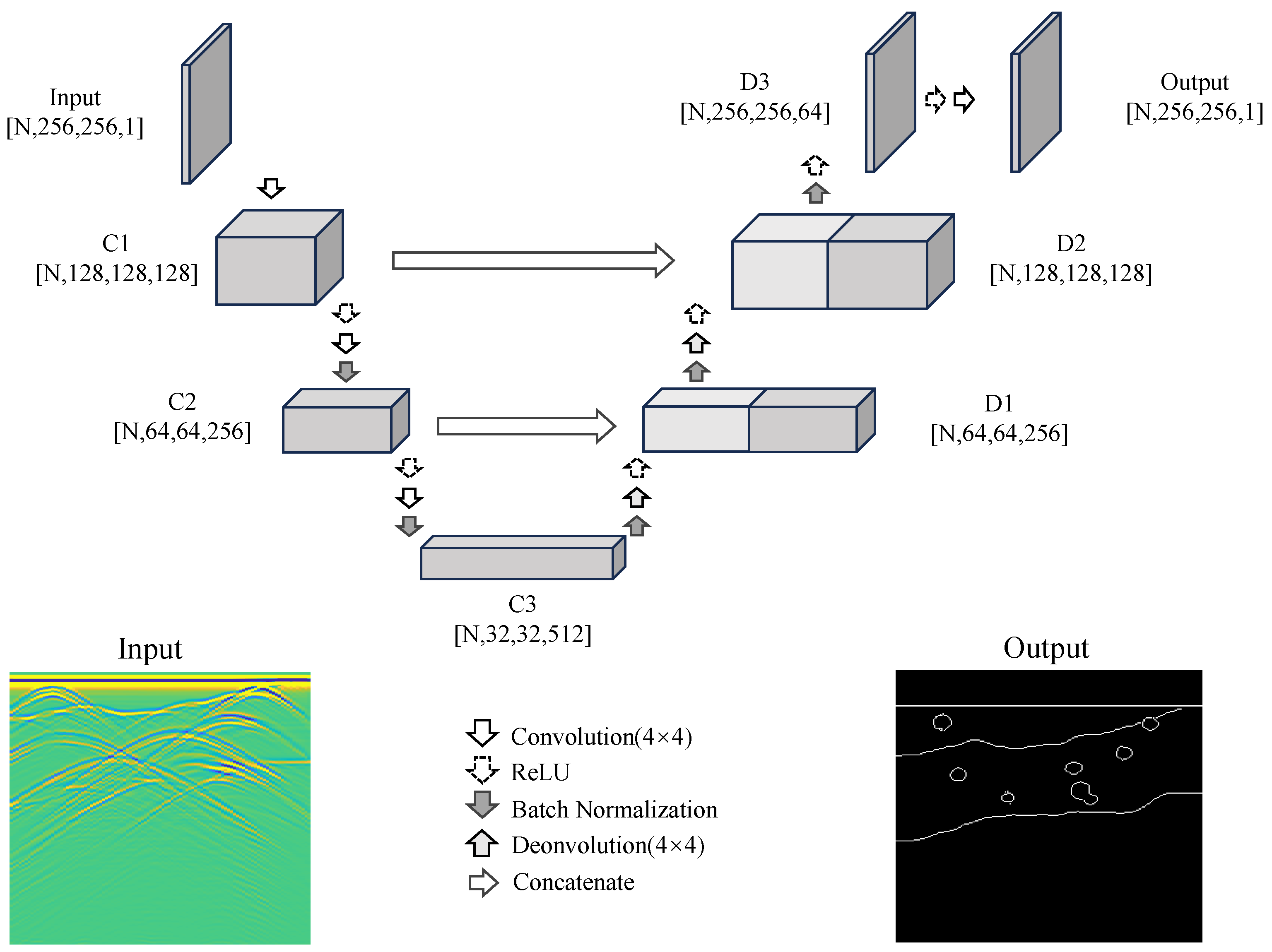
The UNet network, a convolutional neural network architecture designed for image segmentation, excels in feature extraction and processing [24]. This research, driven by a strong commitment to underground exploration and geological studies, utilizes the UNet network to automate the recognition of rock formations and stratigraphic labels in GPR B-scan images, as shown in Figure 3. This has significant strategic importance in accurately detecting subsurface structures and geological features. What sets our proposed UNet network apart is its unique architectural design, incorporating downsampling and upsampling operations along with skip connections. This design enables effective feature capture across a range of scales. For input data, we selected GPR B-scan images sized at 256 × 256 pixels. Using the UNet network, we generated rock and stratigraphic label images of the same dimensions, ensuring a comprehensive representation of subsurface structures. Additionally, a 3 × 3 convolutional kernel was skillfully utilized to extract localized features, allowing the UNet network to discern key elements, such as underground rock formations and stratigraphic layers, with precision.
2.1. Parameters of the Network
Our approach primarily focuses on constructing and training the UNet network. The learning rate was set to 1 × 10⁻⁵, with 300 iterations performed using the Adam optimization algorithm. The learning rate controls how quickly the parameters of a neural network are updated during training. The dataset was divided into 800 training samples, 100 validation samples, and 100 testing samples. Both input and output images have dimensions of 256 × 256 pixels. To supervise the network’s learning process, we employed the L1 loss function to measure the error between predicted values and actual labels. The expression for the L1 loss function is as follows:
Here, represents the true label values, represents the network’s predicted values, and n signifies the number of samples in the dataset. The use of the L1 loss function guides the network’s learning process, gradually reducing the discrepancies between the predicted results and the actual labels, thereby enhancing the network’s performance and accuracy.
2.2. Dataset Generation
The importance of samples in deep learning lies in their role as the foundation for model training and performance evaluation. Sufficiently abundant and diverse samples help deep learning models better comprehend the complexity of a problem, enhancing their generalization capabilities. To simulate the complexity and diversity of underground rock formations and geological structures, we employ stratigraphy generation and rock mass modeling techniques to establish geological models. Subsequently, we utilize the FDTD algorithm to generate radar images, providing high-resolution underground structural data to accurately identify geological features [39,40].
2.2.1. Stratigraphy Generation
The dielectric constant layer model is commonly employed to describe the distribution of dielectric constants within different underground layers, often used in applications such as radar or microwave exploration. The dielectric constant () is typically a dimensionless numerical value. Below is a simplified formula for the dielectric constant layer model, where ’n’ represents the number of layers, and each layer is characterized by distinct dielectric constants () and thicknesses ():
In this formula, denotes the dielectric constant as a function of depth z, and represents summation over the index i for each layer. stands for the dielectric constant of the i-th layer, and represents the thickness of the i-th layer. This formula characterizes the variation of dielectric constants in underground layers.
When constructing complex geological models, incorporating random media is a pivotal step aimed at addressing the heterogeneity and stochastic nature of subsurface materials. This procedure typically encompasses the modeling of random fields and a subsequent statistical analysis [41,42].
Random Field Modeling:
Random fields are mathematical tools used to represent the variation of medium properties with depth or location. A common one-dimensional random field model is the Gaussian random field, described as follows:
where is a random variable at position x, is the mean, and is zero-mean Gaussian white noise with a specific covariance function.
Covariance Function:
The covariance function is used to describe the spatial correlation of random media. Typically, the exponential covariance function is commonly used:
Here, represents the covariance between positions x and y, is the variance, and l is the correlation length parameter. This function indicates the degree of correlation between the properties of the media at different positions.
2.2.2. Rock Mass Modeling
Rock mass modeling is crucial in geological and engineering studies, involving the analysis of subsurface rock structures. Rock masses vary in shape, with circular structures being common. They differ in composition from surrounding media and can appear as discrete underground features. Mathematical and computational methods are used for modeling, often describing rock geometry with geometric equations, such as a formula for a rounded-shape body with radius ‘R’.
Here, ‘x’ and ‘y’ represent the spatial coordinates, and the equation defines a circular boundary with radius ‘R’.
In cases where rock masses exhibit irregular shapes, more complex mathematical functions can be utilized. For example, the equation of an ellipse can be employed to model an elongated rock mass:
In this equation, ‘a’ and ‘b’ represent the semi-major and semi-minor axes, respectively, allowing for flexibility in representing ellipsoidal rock structures.
Furthermore, when modeling rock masses with varying compositions or densities, statistical distributions may be applied. These distributions can describe the probabilistic distribution of rock materials within a given region, offering insights into the heterogeneous nature of subsurface formations.
2.2.3. FDTD Algorithm
Using the FDTD algorithm to simulate GPR observation data is a powerful computational technique. This approach discretizes both space and time into grids and calculates electric and magnetic field values at discrete points. These values are updated based on Maxwell’s equations, enabling the simulation of electromagnetic wave propagation and interaction within the computational domain. In this process, absorbing boundary conditions are typically applied to minimize boundary reflections and enhance simulation accuracy [43,44].
Maxwell’s equations in three-dimensional space are represented as
Electric field update equations:
Magnetic field update equations:
Here, represents the electric field vector, represents the magnetic field vector, is the permittivity, is the permeability, and denotes the curl operator. In the FDTD simulation, these equations are solved iteratively in both space and time, allowing us to model the propagation and reflection of electromagnetic waves in complex dielectric constant models. The application of absorbing boundary conditions mitigates boundary reflections, resulting in more accurate GPR observation data. This numerical simulation method based on FDTD plays a crucial role in subsurface exploration, aiding our understanding of underground structures and geological features [45]. It contributes valuable insights to geological studies and engineering planning by providing a means to analyze subsurface resources and structures more effectively. We utilize the FDTD algorithm to simulate observation data for GPR with absorbing boundary conditions.
To model dielectric constant () distributions, we employ FDTD, which discretizes space and time into a grid. The update equations for the electric (E) and magnetic (H) fields are as follows:
1. Update Equation for Electric Field (E):
2. Update Equation for Magnetic Field (H):
Here, E and H represent the electric and magnetic field components, respectively, at grid points in the 3D grid. and denote the relative permittivity and permeability of the material at that grid point, and is the time step. These equations are applied iteratively in both space and time to simulate the propagation of electromagnetic waves and their interaction with subsurface structures in the GPR model.
For the Y-direction PML boundary conditions,
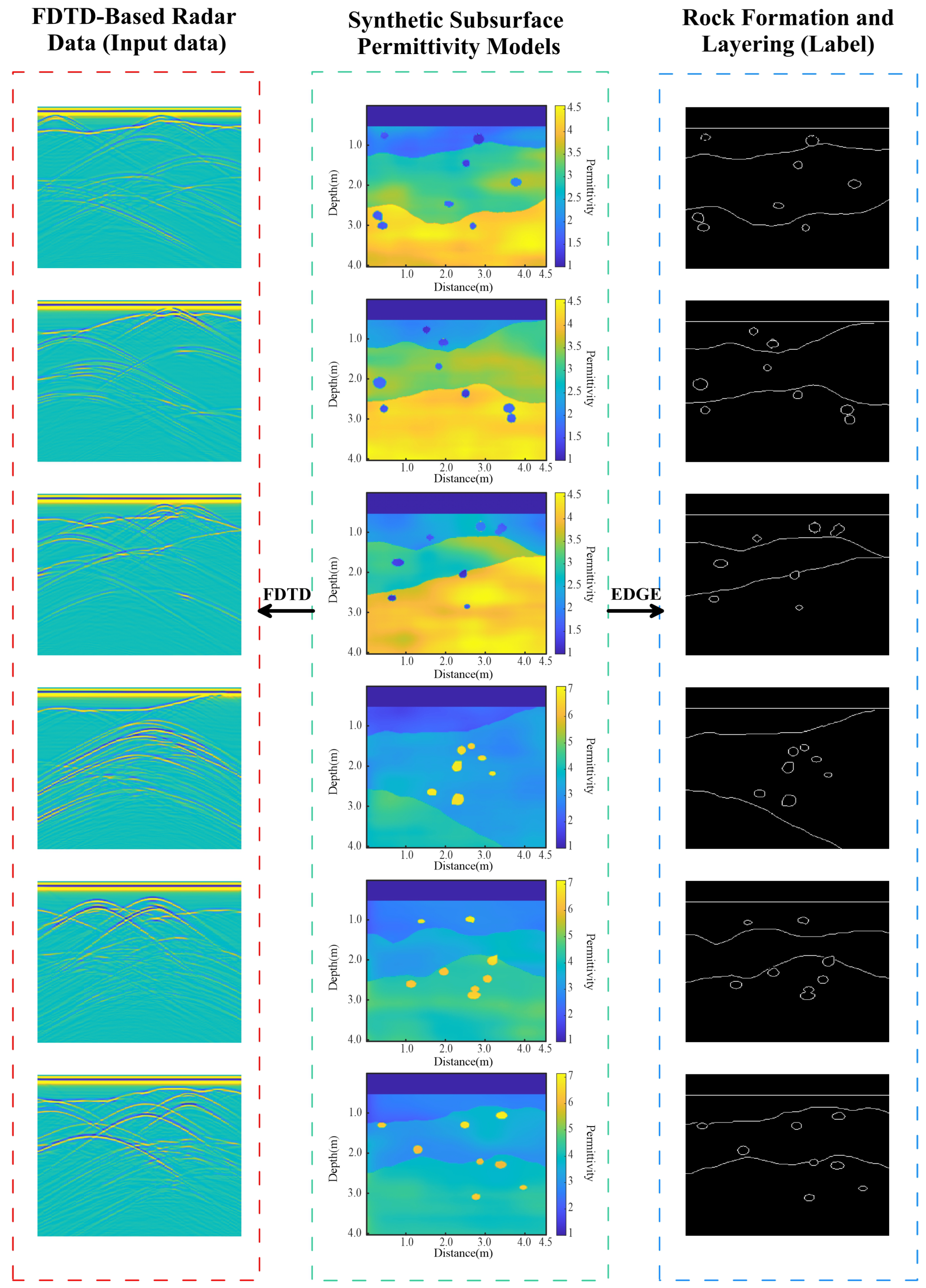
These equations describe the application of PML boundary conditions in two dimensions and cover the electric fields and as well as the magnetic field . Here, i and j represent coordinates in a two-dimensional grid, is the time step, represents the relative permittivity of the material, and and are the spatial step sizes. In this section, we will discuss our methodology, which combines various techniques, including random stratigraphic variation, rock mass generation, stochastic media modeling, and FDTD methods. This approach allows us to create a multitude of irregular dielectric constant sample models and their corresponding radar data. The electrical models derived from these data provide crucial insights into rock formations and stratigraphic structures, as vividly demonstrated in Figure 4.
2.2.4. Dataset Parameters
Our dielectric constant model has a computational domain size of 4.5 m by 4 m, divided into a grid of 180 by 160 cells. The main frequency of the GPR is 600 MHz. The number of sources is 101, with a spacing of 0.045 m. The time step is set to 0.501 × 10⁻¹¹ s. The source is located at a depth of 0.5 m and employs a self-excitation and self-reception mode. The observation points coincide with the source location. To minimize boundary reflections, we utilize PML boundary conditions. The simulation time is set to 0.5 × 10⁻⁷ s. The numerical values of the dielectric constant model typically range from 1 to 8, reflecting typical shallow subsurface structural features. The values of the label data usually range from 0 to 1, with a value of 1 representing locations of blocks and layers, and a value of 0 indicating positions without distinct structures. After obtaining the input and output data, we used the “imresize” command to resize them into a 256 × 256 matrix to meet the prediction requirements of the UNet network.
3. Results
This study includes experiments with synthetic data and field data. Synthetic data experiments involve datasets generated by us, while field data were obtained from real-world measurements.
3.1. Synthetic Data
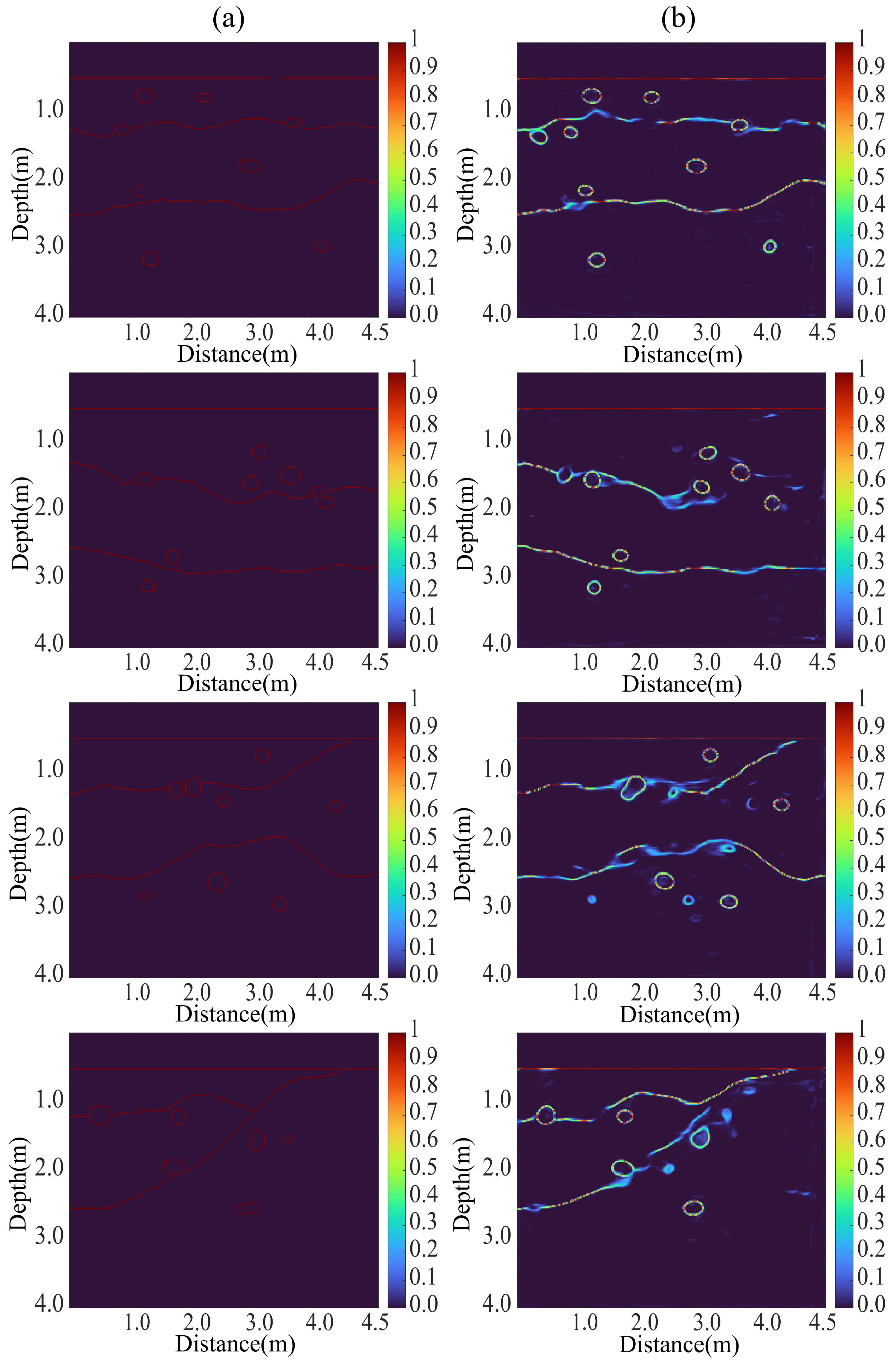
Figure 5 showcases four sets of deep learning predictions, revealing the results of predicting underground rock and stratigraphic structures using the UNet architecture for GPR data. By juxtaposing the predicted images on the left with the ground truth images on the right, we can thoroughly assess the model’s performance [46]. The deep neural network takes 12 h to train, yet its prediction speed is less than 1 s. Therefore, once the training is complete, the network model can be deployed immediately.
Initially, it is apparent that the predictions on the left closely resemble the ground truth images on the right in terms of color distribution and the continuity of stratigraphic structures. Clear boundaries of stratigraphic layers are discernible in the left images, mirroring their presence in the ground truth images. This confirms the UNet model’s ability to accurately capture the structural characteristics of subterranean rock layers and generate reasonably precise stratigraphic distribution maps based on this understanding. Moreover, the model excels in identifying and reproducing larger structural features within the rock layers, such as prominent boundaries and rock formations. While these features, depicted by deeper hues in the ground truth images, are similarly reflected in the prediction results, there may be minor deviations in fine-grained details. In certain cases, the prediction results accurately depict the shapes of these structures, although precision in terms of size and positioning may vary.
Nonetheless, it is worth noting that disparities between the prediction results and ground truth emerge in certain finer details. For instance, some minor features within the rock layers may appear as blurred or omitted in the predictions. Such occurrences could be attributed to the model’s constrained generalization capacity or the limited presence of samples featuring these particular characteristics in the training data. Additionally, in select stratigraphic layers, disruptions in the prediction results hint at opportunities for enhancement concerning the model’s ability to capture the continuity of subterranean structures. A commendable aspect of the model is its proficiency in preserving the overall trends of the stratigraphic layers. In most prediction images, the model successfully tracks the general trends of these layers, a valuable trait for subsurface exploration. This suggests that despite occasional deviations in specific details, the model’s predictions continue to offer invaluable insights into subterranean structures.
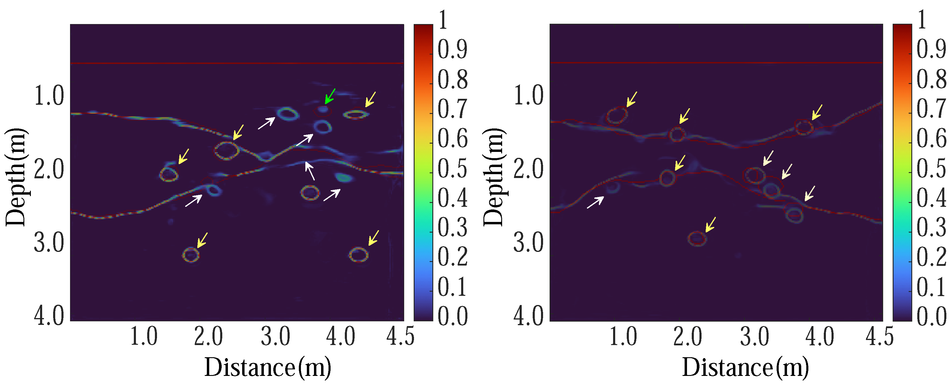
Displayed in Figure 6, these two images depict the prediction outcomes following the processing of GPR data using the deep learning model UNet, accompanied by a comparative overlay with the ground truth. Within each image, the anticipated signals related to subterranean rock and stratigraphic structures are conveyed through varying color intensities, symbolizing the likelihood of their presence. Concurrently, actual rock and stratigraphic structures are superimposed in a semi-transparent layer atop the prediction results. By scrutinizing the accuracy of predictions and identifying discrepancies (where yellow arrows denote correct predictions and white arrows pinpoint inaccuracies), we can evaluate the model’s performance.
Firstly, based on the provided information, the model demonstrates a commendable accuracy rate, precisely predicting 88% of the rock formations. This remarkable level of precision implies that the model can consistently identify and forecast underground structures in the majority of cases. Such highly accurate predictions are invaluable for geologists and engineers involved in underground exploration and assessment, as they can effectively mitigate risks and minimize costs associated with on-site surveys. Upon a closer examination of the yellow arrows in the images, it becomes evident that these arrows typically point towards areas with deeper colors, corresponding to respective segments of the ground truth layers, thus indicating a heightened probability of accurate prediction signals. The presence of green arrows signifies false weak anomalies, potentially influencing judgment, although their quantity can be maintained within acceptable limits. This suggests that in these areas, the prediction model can accurately capture the presence and morphology of underground rock formations with exceptional precision. Nonetheless, instances of prediction errors, as denoted by the white arrows in the images, also exist. These errors may arise from the model’s failure to capture all intricate geological features or insufficient acquisition of these features during the training process. Such prediction inaccuracies could be attributed to an inadequate training dataset or the complexity of the underground rock layers surpassing the model’s processing capabilities.
Overall, these prediction results underscore the remarkable potential of the UNet model in handling GPR data. High-accuracy predictions provide invaluable insights for exploring and developing underground resources while pinpointing areas where the model may require improvements under specific circumstances.
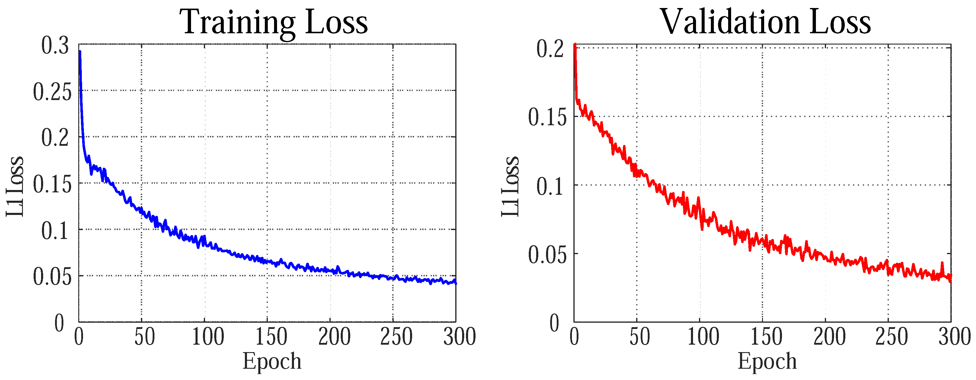
As illustrated in Figure 7, in the left image, we can observe a decreasing trend in the training loss function of the UNet network as the number of epochs increases. This trend signifies that as the training progresses, the network steadily enhances its performance and acquires a deeper understanding of the features present in GPR signals related to underground rock and stratigraphic structure information. Initially, the training loss curve exhibits a steep decline, which is often indicative of the network’s rapid learning from the data. However, with the passage of time, the rate of loss reduction gradually decelerates, suggesting that the network might be approaching the limits of its learning capacity and potentially entering a convergent state.
The right image presents the loss function on the validation set. Similarly, the loss function diminishes as the number of epochs increases, a positive indication that the model generalizes effectively to previously unseen data. The decreasing trend in validation loss remains relatively stable in comparison to the training loss, without any noticeable upward trends, implying the absence of overfitting and affirming the model’s strong generalization capabilities [47].
In summary, these two loss function graphs showcase the exceptional performance of the UNet network over the course of 300 training epochs. Both training and validation losses exhibit a consistently declining trend, with no indications of overfitting. This underscores the model’s high effectiveness in predicting underground rock and stratigraphic structure information from GPR signals while demonstrating sound generalization capabilities.
3.2. Measured Data
During the actual data collection process, we utilized a GPR with a central frequency of 600 MHz, specifically the SIR-3000 model. The waveform type employed was the Ricker wavelet, with vertical polarization being the polarization mode. The acquisition system comprised a transmitter (antenna), receiver (antenna), control unit (responsible for controlling the transmission and reception processes, as well as recording data), and data processing unit (utilized for processing and analyzing the collected data, generating underground structure images or profiles). The field setting chosen was a flat and obstacle-free open area.
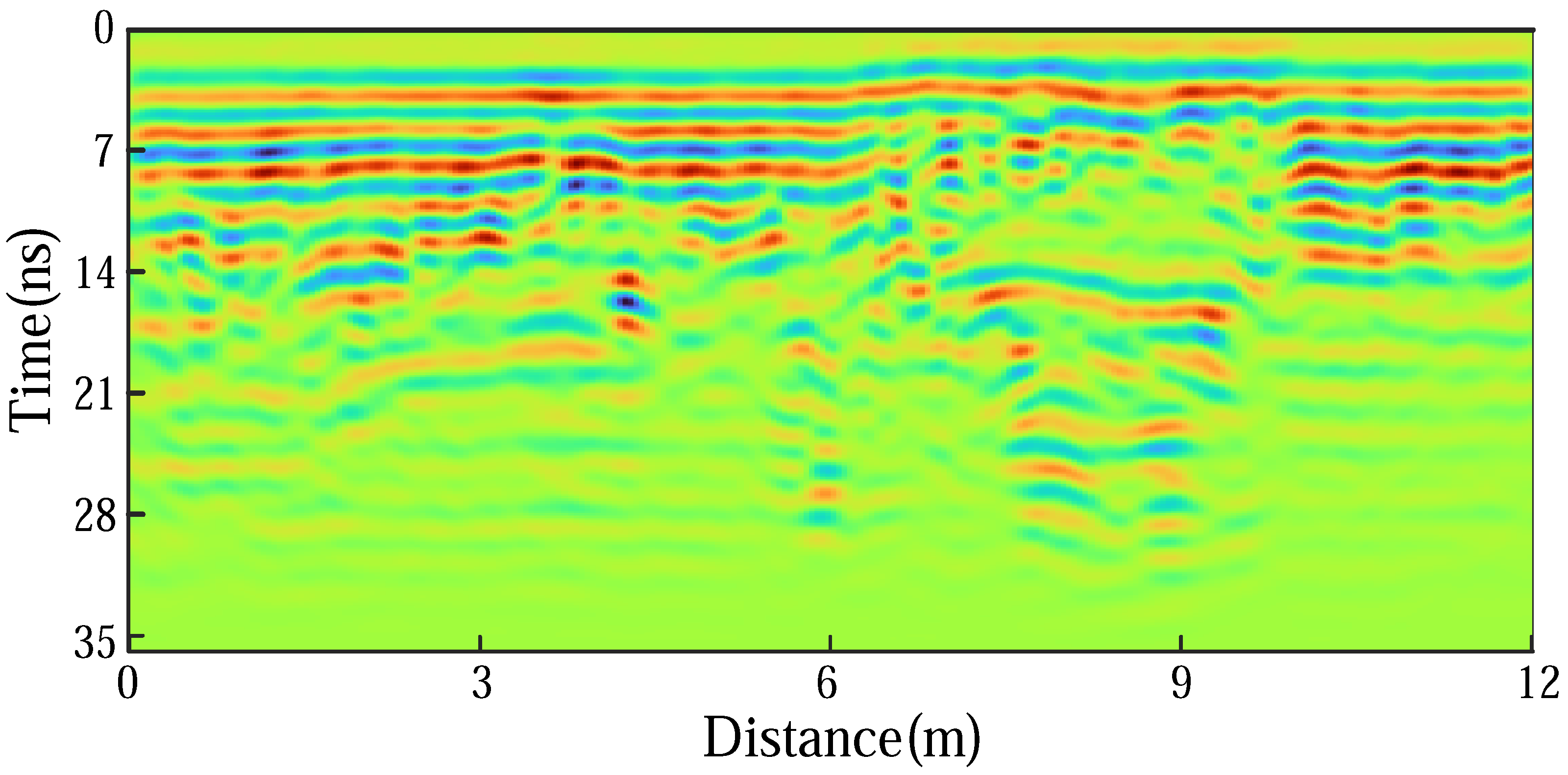
Figure 8 displays a measured GPR data image. In the image, radar signals are represented in color, where different colors indicate varying signal strengths. The time depth is 35 nanoseconds (ns), and the survey length is approximately 16 m. Radar data are typically used to analyze subsurface structural features, such as rock layers, voids, or other obstacles.
Initial observations are focused on the horizontal colored stripes, likely representing underground stratigraphic structures. Red and yellow areas indicate strong reflection signals, suggesting differences in underground interfaces or material electrical properties, while green and blue areas show weaker signals, possibly due to more homogeneous underground materials or enhanced signal penetration capabilities. Signal continuity varies at different depths, with clearer signals near the surface possibly reflecting harder rock layers or lower water content, while decreased continuity and clarity at greater depths may result from more complex underground materials or increased water content, leading to more complex radar signal reflections and refractions.
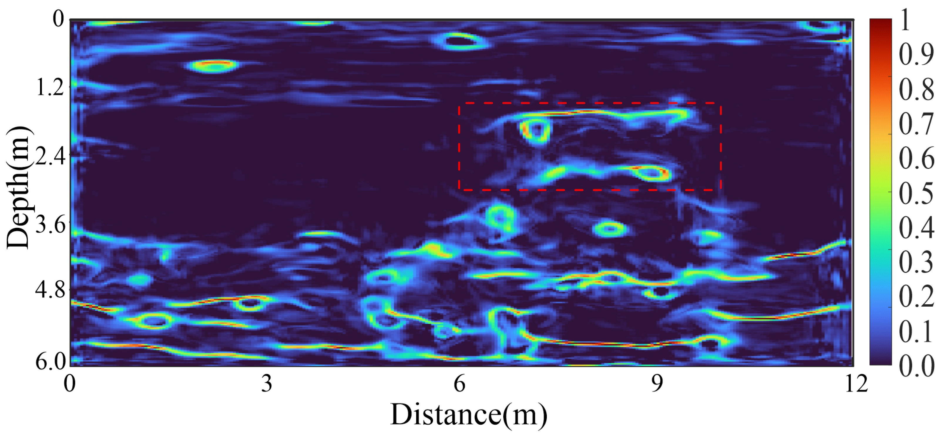
Figure 9 presents prediction results of measured GPR data obtained through a well-trained UNet neural network. Image color intensity indicates the probability of underground rock and stratigraphic structure information. Circular markers represent potential rock formations or blocks, and continuous signals may indicate geological strata. These analyses provide insights into the practical application of deep learning in geological exploration.
First and foremost, the image shows multiple bright spots, variations in color intensity, and the presence of circular markers, suggesting potential locations of rock formations or blocks. Identifying these features is crucial for guiding subterranean resource exploration, as they could indicate the presence of metal pipes, boulders, or other geological anomalies. Additionally, the continuous signals in the image, depicted as elongated color bands, indicate the persistent structure of geological strata. It is noteworthy that these continuous signals exhibit varying strengths at different depths, likely due to variations in the physical properties of the strata, such as soil moisture, density, or material composition disparities.
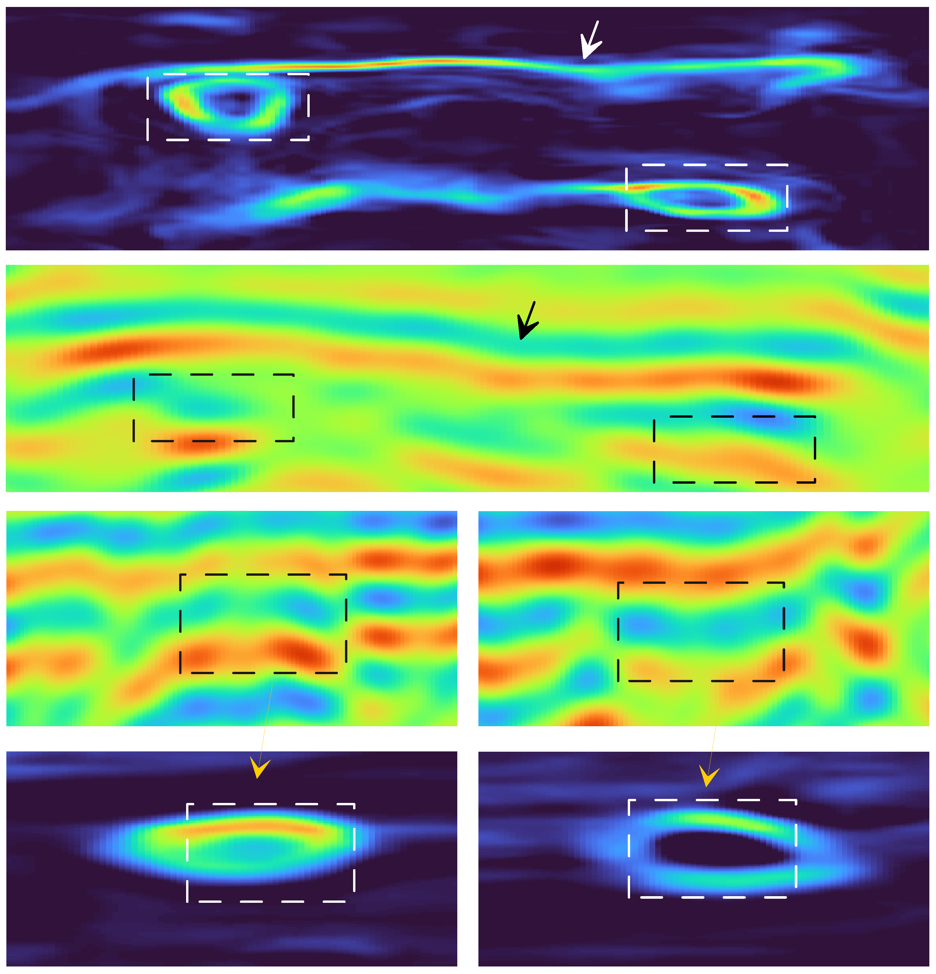
Figure 10 presents a localized comparison between the prediction results obtained using the UNet network’s processing of real GPR data and the original radar signals. The consistency between the radar signals outlined by black boxes and the prediction results enclosed in white boxes underscores the model’s precision in stratal coherence and stratigraphic recognition. Analyzing these images provides a deeper insight into the application and effectiveness of deep learning in identifying geological structures. To begin, from the enlarged images, it becomes evident that the prediction results (white boxes) closely correspond to the structural characteristics of the actual radar data (black boxes). This consistency highlights the UNet’s capacity to accurately learn the features of underground rock layers from GPR data and predict their structures. Notably, this capability is particularly evident in recognizing stratal coherence, which manifests as continuous curves in GPR images and plays a crucial role in indicating electromagnetic property variations among different materials. The regions indicated by arrows showcase the model’s potential application in complex geological environments. In these areas, even as geological structures become more intricate, the prediction results maintain a robust correlation with the measured data. This demonstrates that the UNet model can not only identify simple layer structures but also handle more complex geological scenarios.
Moreover, these enlarged views allow us to observe the model’s ability to capture intricate features of underground rock layers. For instance, the model can depict minor bends and subtle density variations within stratigraphy, which are essential for precise geological exploration. In summary, these comparative images highlight the UNet model’s high accuracy and substantial potential in predicting underground rock layers and stratigraphic structures. The remarkable consistency displayed within the black and white boxes underscores the model’s competence in extracting and learning geological features. This not only validates the practicality of deep learning technology in geological exploration but also furnishes a potent tool for future geological structure analyses and resource exploration [48]. With further training and optimization, these models are poised to make significant advancements in handling more complex geological data, providing geologists and exploration engineers with more detailed and accurate underground information.
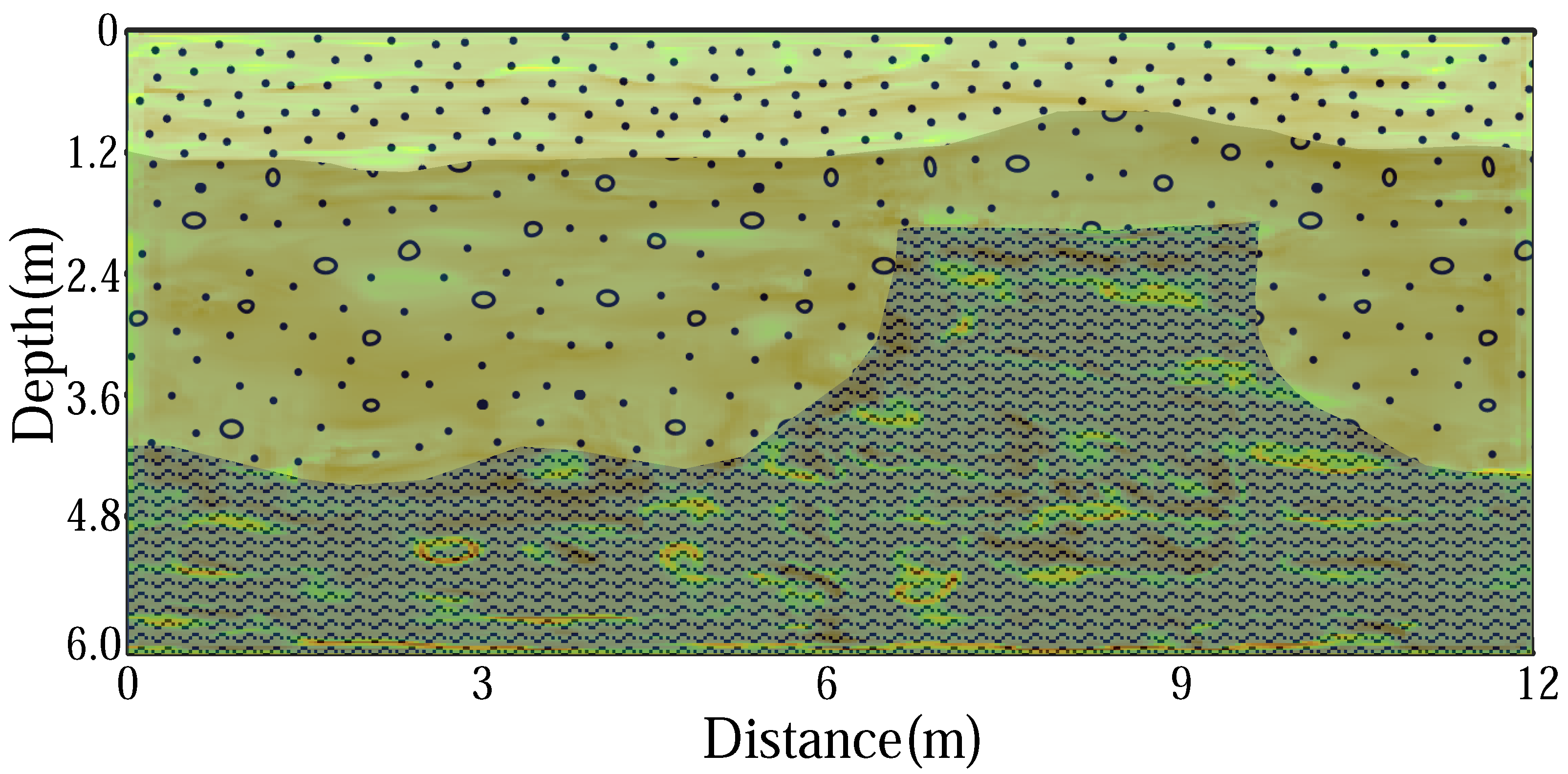
Figure 11 illustrates the underground structure, as predicted and explained by the UNet. The image reveals that the surface layer comprises sandy soil, depicted as a relatively uniform light-colored region. Within this sandy soil layer, there are scattered small rocks or blocks, potentially indicating the presence of gravel or larger sand particles beneath the surface. Beneath the sandy soil layer lies a layer of clay, identifiable by its darker hue in contrast to the sandy soil layer. This disparity suggests distinct physical properties in this layer, which could be attributed to variations in clay moisture, density, or other mineral components causing alterations in reflectance [49]. The clay layer exhibits a discernible thickness, with the color gradually deepening as depth increases, possibly signifying changes in both thickness and material composition within the clay layer. The lowest layer comprises bedrock, appearing as a more uniform and continuous color zone in the image. This bedrock layer exhibits a harder and more consistently structured nature, contrasting sharply with the sediment layers above it.
4. Discussion
The precise identification of underground rock formations and stratigraphic structures holds paramount importance in geological exploration and engineering construction, facilitating risk mitigation and cost reduction. While traditional manual feature extraction methods are often time-consuming and laborious, deep learning models offer the automated learning and extraction of complex underground structural features, thereby enhancing identification accuracy and efficiency. Consequently, this study aims to achieve the precise identification of underground rock layers and stratigraphic structures by integrating GPR technology with a deep learning model.
Initially, we employed Random Field Modeling and stratigraphy generation techniques to generate 1000 models of dielectric constants with randomly undulating layers and randomly distributed rock blocks. These models’ dielectric constants mirrored actual conditions and varied between 1 and 8. Subsequently, we numerically simulated the dielectric constant models using the FDTD method, yielding corresponding radar images. By combining radar images with rock layer position information, we established data pairs and utilized the UNet network to learn the mapping relationship between radar images and rock layer labels.
Throughout 300 epochs, the training duration was approximately 12 h, with the loss functions of the training set and validation set exhibiting a stable decreasing trend. The trained deep network required less than 1 s to predict the test set. The network’s prediction results indicated an 88% match with the ground truth regarding rock information, albeit with some discontinuities in the layer structure information, possibly due to signal loss from excessive rock blocks. Overall, the fluctuation characteristics and burial depth of the layer information closely resembled the actual situation.
Finally, we employed field data consistent with synthetic data parameters for prediction, obtained from a flat and obstacle-free open area. The prediction results demonstrated a moderate number of surface rock formations, fewer formations in the middle area, and increased formations at greater depths. Additionally, coherence information in the middle and deep areas was evident. Based on these prediction results, we analyzed the stratigraphic structure of the area. The imagery revealed a surface layer comprising sandy soil, depicted as a relatively uniform light-colored region, with scattered small rocks or blocks potentially indicating gravel or larger sand particles beneath the surface. Below the sandy soil layer lay a layer of clay, distinguishable by its darker hue compared to the sandy soil layer.
5. Conclusions
In conclusion, this study demonstrates the effectiveness of integrating GPR with the UNet deep learning model for identifying underground rock formations and stratigraphic structures. The consistency between GPR-derived signals and UNet’s predictions underscores the model’s accuracy in recognizing stratigraphic coherence and geological features. These findings validate previous research on GPR’s potential in subsurface characterization and highlight the efficacy of incorporating deep learning techniques like UNet into GPR data processing for geological exploration. The implications of these results extend to various fields, including geological resource assessment, environmental monitoring, and civil engineering applications. The successful application of UNet in complex geological environments suggests potential for future research and exploration methodologies. Future directions may involve enhancing the model’s robustness, optimizing data acquisition strategies, and further validating predictions through field studies. Overall, this study emphasizes the synergistic role of GPR and UNet as valuable tools in geological investigation and provides insights into potential avenues for future research and application.
Author Contributions
Resources, H.X.; Data curation, Z.J., P.J. and H.X.; Writing—original draft, H.X., J.Y. and G.F.; Writing—review and editing, J.Y., H.X. and Z.J.; Supervision, G.F.; Project administration, G.F. and H.X. All authors have read and agreed to the published version of the manuscript.
Funding
The authors gratefully acknowledge the financial support from the National Natural Science Foundation of China (52208330, 42177168), Natural Science Foundation of Hunan Province (2022JJ40500), and Open Fund of Key Laboratory of Safety Control of Bridge Engineering, Ministry of Education (Changsha University of Science and Technology) (21KB13).
Data Availability Statement
The data presented in this study are available on request from the corresponding author. The data are not publicly available due to privacy.
Conflicts of Interest
The authors declare no conflicts of interest.
Abbreviations
The following abbreviations are used in this manuscript:
| FDTD | Finite-Difference Time-Domain |
| CNN | Convolutional Neural Network |
| GPR | Ground-penetrating Radar |
| ns | Nanoseconds |
| UNET | U-shaped Network |
References
- Ambrosanio, M.; Bevacqua, M.T.; Isernia, T.; Pascazio, V. The tomographic approach to ground-penetrating radar for underground exploration and monitoring: A more user-friendly and unconventional method for subsurface investigation. IEEE Signal Process. Mag. 2019, 36, 62–73. [Google Scholar] [CrossRef]
- Gizzi, F.T.; Leucci, G. Global research patterns on ground penetrating radar. Surv. Geophys. 2018, 39, 1039–1068. [Google Scholar] [CrossRef]
- Zhao, W.; Forte, E.; Pipan, M.; Tian, G. Ground penetrating radar (GPR) attribute analysis for archaeological prospection. J. Appl. Geophys. 2013, 97, 107–117. [Google Scholar] [CrossRef]
- Benedetto, A.; Tosti, F.; Ciampoli, L.B.; D’Amico, F. GPR applications across engineering and geosciences disciplines in Italy: A review. IEEE J. Sel. Top. Appl. Earth Obs. Remote Sens. 2016, 9, 2952–2965. [Google Scholar] [CrossRef]
- Di Prinzio, M.; Bittelli, M.; Castellarin, A.; Pisa, P.R. Application of GPR to the monitoring of river embankments. J. Appl. Geophys. 2010, 71, 53–61. [Google Scholar] [CrossRef]
- Pryshchenko, O.A.; Plakhtii, V.; Dumin, O.M.; Pochanin, G.P.; Ruban, V.P.; Capineri, L.; Crawford, F. Implementation of an Artificial Intelligence Approach to GPR Systems for Landmine Detection. Remote Sens. 2022, 14, 4421. [Google Scholar] [CrossRef]
- Küçükdemirci, M.; Sarris, A. GPR data processing and interpretation based on artificial intelligence approaches: Future perspectives for archaeological prospection. Remote Sens. 2022, 14, 3377. [Google Scholar] [CrossRef]
- Witten, A.J.; Molyneux, J.E.; Nyquist, J.E. Ground penetrating radar tomography: Algorithms and case studies. IEEE Trans. Geosci. Remote Sens. 1994, 32, 461–467. [Google Scholar] [CrossRef]
- Lombardi, F.; Podd, F.; Solla, M. From its core to the niche: Insights from GPR applications. Remote Sens. 2022, 14, 3033. [Google Scholar] [CrossRef]
- Annan, A.P. Ground-penetrating radar. In Near-Surface Geophysics; Society of Exploration Geophysicists: Houston, TX, USA, 2005; pp. 357–438. [Google Scholar]
- Arosio, D. Rock fracture characterization with GPR by means of deterministic deconvolution. Journal of Applied Geophysics. J. Appl. Geophys. 2016, 126, 27–34. [Google Scholar] [CrossRef]
- Elkarmoty, M.; Colla, C.; Gabrielli, E.; Bonduà, S.; Bruno, R. Deterministic three-dimensional rock mass fracture modeling from geo-radar survey: A case study in a sandstone quarry in Italy. Environ. Eng. Geosci. 2017, 23, 314–331. [Google Scholar] [CrossRef]
- Grandjean, G.; Gourry, J.C.; Bitri, A. Evaluation of GPR techniques for civil-engineering applications: Study on a test site. J. Appl. Geophys. 2000, 45, 141–156. [Google Scholar] [CrossRef]
- Knight, R. Ground penetrating radar for environmental applications. Annu. Rev. Earth Planet. Sci. 2001, 29, 229–255. [Google Scholar] [CrossRef]
- Jia, Z.; Li, Y.; Lu, W.; Zhang, L.; Monkam, P. EMRNet: End-to-end electrical model restoration network. IEEE Trans. Geosci. Remote Sens. 2022, 60, 1–12. [Google Scholar] [CrossRef]
- Neal, A. Ground-penetrating radar and its use in sedimentology: Principles, problems and progress. Earth-Sci. Rev. 2004, 66, 261–330. [Google Scholar] [CrossRef]
- Jol, H.M.; Smith, D.G.; Meyers, R.A. Digital ground penetrating radar (GPR): A new geophysical tool for coastal barrier research (examples from the Atlantic, Gulf and Pacific Coasts, USA). J. Coast. Res. 1996, 12, 960–968. [Google Scholar]
- Kaur, P.; Dana, K.J.; Romero, F.A.; Gucunski, N. Automated GPR rebar analysis for robotic bridge deck evaluation. IEEE Trans. Cybern. 2015, 46, 2265–2276. [Google Scholar] [CrossRef] [PubMed]
- Xu, X.; Zeng, Q.; Li, D.; Wu, J.; Wu, X.; Shen, J. GPR detection of several common subsurface voids inside dikes and dams. Eng. Geol. 2010, 111, 31–42. [Google Scholar] [CrossRef]
- Slob, E.; Sato, M.; Olhoeft, G. Surface and borehole ground-penetrating-radar developments. Geophysics 2010, 75, 75A103–75A120. [Google Scholar] [CrossRef]
- Davis, J.L.; Annan, A.P. Ground-penetrating radar for high-resolution mapping of soil and rock stratigraphy 1. Geophys. Prospect. 1989, 37, 531–551. [Google Scholar] [CrossRef]
- Liu, L.B.; Qian, R.Y. Ground Penetrating Radar: A critical tool in Near Surf. Geophys. Chin. J. Geophys. 2015, 58, 2606–2617. [Google Scholar]
- Jia, Z.; Li, Y.; Wang, Y.; Li, Y.; Jin, S.; Li, Y.; Lu, W. Deep Learning for 3-D Magnetic Inversion. IEEE Trans. Geosci. Remote Sens. 2023, 61, 1–10. [Google Scholar] [CrossRef]
- Jia, Z.; Wang, Y.; Li, Y.; Xu, C.; Wang, X.; Lu, W. Magnetotelluric Closed-Loop Inversion. IEEE Trans. Geosci. Remote Sens. 2023, 61, 1–11. [Google Scholar] [CrossRef]
- Zheng, Y.; Wang, Y. Ground-penetrating radar wavefield simulation via physics-informed neural network solver. Eng. Geol. 2023, 88, KS47–KS57. [Google Scholar] [CrossRef]
- Liu, P.; Cao, N.; Zhang, Z.; Zhang, T.; Yang, Y. Deep learning of ground penetrating radar data inversion in reinforcement detection domain. Prog. Geophys. 2023, 38, 1355–1365. [Google Scholar]
- Qin, T.; Bohlen, T.; Allroggen, N. Full-waveform inversion of ground-penetrating radar data in frequency-dependent media involving permittivity attenuation. Geophys. J. Int. 2023, 232, 504–522. [Google Scholar] [CrossRef]
- Ebraheem, M.O.; Ibrahim, H.A. A comprehensive study of some features from characteristics of enhanced ground-penetrating radar wave images through convenient data processing within carbonate rock, west of Assiut, Egypt. Geophys. Prospect. 2023, 71, 495–506. [Google Scholar] [CrossRef]
- Zhong, S.; Wang, Y.; Zheng, Y. Frequency-domain wavefield reconstruction inversion of ground-penetrating radar based on sensitivity analysis. Geophys. Prospect. 2023, 71, 1655–1672. [Google Scholar] [CrossRef]
- Amaya, M.; Meles, G.; Marelli, S.; Linde, N. Multifidelity adaptive sequential Monte Carlo for geophysical inversion. Geophys. J. Int. 2024, 237, 788–804. [Google Scholar] [CrossRef]
- Tong, Z.; Gao, J.; Yuan, D. Advances of deep learning applications in ground-penetrating radar: A survey. Constr. Build. Mater. 2020, 258, 120371. [Google Scholar] [CrossRef]
- Hou, F.; Lei, W.; Li, S.; Xi, J. Deep learning-based subsurface target detection from GPR scans. IEEE Sens. J. 2021, 21, 8161–8171. [Google Scholar] [CrossRef]
- Liu, B.; Ren, Y.; Liu, H.; Xu, H.; Wang, Z.; Cohn, A.; Jiang, P. GPRInvNet: Deep learning-based ground-penetrating radar data inversion for tunnel linings. IEEE Trans. Geosci. Remote Sens. 2021, 59, 8305–8325. [Google Scholar] [CrossRef]
- Li, Y.; Weng, A.; Xu, W.; Zou, Z.; Tang, Y.; Zhou, Z.; Li, S.; Zhang, Y.; Ventura, G. Translithospheric magma plumbing system of intraplate volcanoes as revealed by electrical resistivity imaging. Geology 2021, 49, 1337–1342. [Google Scholar] [CrossRef]
- Yuan, W.; Liu, S.; Zhao, Q.; Deng, L.; Lu, Q.; Pan, L.; Li, Z. Application of Ground-Penetrating Radar with the Logging Data Constraint in the Detection of Fractured Rock Mass in Dazu Rock Carvings, Chongqing, China. Remote Sens. 2023, 15, 4452. [Google Scholar] [CrossRef]
- Yuan, H.; Abdu, A.Z.; Nielsen, L. Prediction of porosity and water saturation of chalks from combined refraction seismic and reflection ground-penetrating radar measurements. Eng. Geol. 2023, 88, MR141–MR153. [Google Scholar] [CrossRef]
- Caselle, C.; Bonetto, S.; Comina, C.; Stocco, S. GPR surveys for the prevention of karst risk in underground gypsum quarries. Tunn. Under. Space Tech. 2020, 95, 103137. [Google Scholar] [CrossRef]
- Duan, M.; Li, K.; Yang, C.; Li, K. A hybrid deep learning CNN–ELM for age and gender classification. Neurocomputing 2018, 275, 448–461. [Google Scholar] [CrossRef]
- Zajícová, K.; Chuman, T. Application of ground penetrating radar methods in soil studies: A review. Geoderma 2019, 343, 116–129. [Google Scholar] [CrossRef]
- Benson, A.K. Applications of ground penetrating radar in assessing some geological hazards: Examples of groundwater contamination, faults, cavities. J. Appl. Geophys. 1995, 33, 177–193. [Google Scholar] [CrossRef]
- Economou, N.; Benedetto, F.; Bano, M.; Tzanis, A.; Nyquist, J.S.; Sandmeier, K.J.; Cassidy, N. Advanced ground penetrating radar signal processing techniques. Signal Process. 2017, 132, 197–200. [Google Scholar] [CrossRef]
- Yuan, H.; Montazeri, M.; Looms, M.C.; Nielsen, L. Diffraction imaging of ground-penetrating radar data. Eng. Geol. 2019, 84, H1–H12. [Google Scholar] [CrossRef]
- Allroggen, N.; Heincke, B.; Koyan, P.; Wheeler, W.; Rønning, J. 3D ground-penetrating radar attribute classification: A case study from a paleokarst breccia pipe in the Billefjorden area on Spitsbergen, Svalbard. Geophysics 2022, 87, WB19–WB30. [Google Scholar] [CrossRef]
- Fu, L.; Liu, S.; Liu, L.; Lei, L. Development of an airborne ground penetrating radar system: Antenna design, laboratory experiment, and numerical simulation. IEEE J. Sel. Top. Appl. Earth Obs. Remote Sens. 2014, 7, 761–766. [Google Scholar] [CrossRef]
- Leucci, G.; De Giorgi, L. Microgravimetric and ground penetrating radar geophysical methods to map the shallow karstic cavities network in a coastal area (Marina Di Capilungo, Lecce, Italy). Explor. Geophys. 2010, 41, 178–188. [Google Scholar] [CrossRef]
- Gao, K.; Donahue, C.; Henderson, B.G.; Modrak, R.T. Deep-learning-guided high-resolution subsurface reflectivity imaging with application to ground-penetrating radar data. Geophys. J. Int. 2023, 233, 448–471. [Google Scholar] [CrossRef]
- Simaiya, S.; Lilhore, U.K.; Sharma, Y.K.; Rao, K.B.; Maheswara Rao, V.V.R.; Baliyan, A.; Bijalwan, A.; Alroobaea, R. A hybrid cloud load balancing and host utilization prediction method using deep learning and optimization techniques. Sci. Rep. 2024, 14, 1337. [Google Scholar] [CrossRef] [PubMed]
- Ardekani, M.; Lambot, S. Full-wave calibration of time-and frequency-domain ground-penetrating radar in far-field conditions. IEEE Trans. Geosci. Remote Sens. 2013, 51, 664–678. [Google Scholar]
- He, T.; Peng, S.; Cui, X.; Zheng, Y.; Shi, Z. An advanced instantaneous frequency method for ground-penetrating radar cavity detection. J. Appl. Geophys. 2023, 212, 104993. [Google Scholar] [CrossRef]
Figure 1.
Ground-penetrating radar detection principle and data imaging schematic; the ground-penetrating radar working system (a) receives instructions and generates ground-penetrating radar 1D signals (b), which are then processed to produce ground-penetrating radar 2D images (c).
Figure 1.
Ground-penetrating radar detection principle and data imaging schematic; the ground-penetrating radar working system (a) receives instructions and generates ground-penetrating radar 1D signals (b), which are then processed to produce ground-penetrating radar 2D images (c).

Figure 2.
A schematic for information extraction from ground-penetrating radar images using CNN.

Figure 3.
A conceptual diagram of rock formation prediction in ground-penetrating radar images using full CNN-based UNet. Convolution is a mathematical operation used to apply filters on images or signals to extract features. ReLU (Rectified Linear Unit) is an activation function that sets negative values to zero, enhancing the non-linear properties of neural networks. Deconvolution is a process used to restore low-dimensional feature maps to high-dimensional original inputs. By applying convolutional kernels on feature maps and adjusting size through padding and stride, deconvolution expands spatial dimensions of feature maps, thereby restoring the original input size and shape.

Figure 4.
Conceptual representation of dielectric constant model, radar data, and label images, where radar data serve as input, and rock structure labels as output.
Figure 4.
Conceptual representation of dielectric constant model, radar data, and label images, where radar data serve as input, and rock structure labels as output.

Figure 5.
A comparative visualization of predictions on synthetic data using a trained UNet model against ground truth. (a) represents the expected output, also known as the ground truth. (b) represents the prediction results of the trained deep neural network, with the color scale indicating probabilities. It can be observed that in (a), positions with a value of 1 usually represent structural information, and in (b), most structural information can be predicted well, with some values also being very close to the ground truth.

Figure 6.
Observation image after overlapping network predictions with ground truth.

Figure 7.
Loss curve plots for training and validation sets during the network training process.

Figure 8.
The measured ground-penetrating radar data detected and utilized in this study.

Figure 9.
Network predictions corresponding to measured observational radar data.

Figure 10.
Schematic for comparative analysis between network predictions enhanced by local zooming and radar data. The structures in the image correspond to the red dashed box area in Figure 9.
Figure 10.
Schematic for comparative analysis between network predictions enhanced by local zooming and radar data. The structures in the image correspond to the red dashed box area in Figure 9.

Figure 11.
Schematic geological interpretation based on network prediction results.

Disclaimer/Publisher’s Note: The statements, opinions and data contained in all publications are solely those of the individual author(s) and contributor(s) and not of MDPI and/or the editor(s). MDPI and/or the editor(s) disclaim responsibility for any injury to people or property resulting from any ideas, methods, instructions or products referred to in the content. |
© 2024 by the authors. Licensee MDPI, Basel, Switzerland. This article is an open access article distributed under the terms and conditions of the Creative Commons Attribution (CC BY) license (https://creativecommons.org/licenses/by/4.0/).
Share and Cite
MDPI and ACS Style
Xu, H.; Yan, J.; Feng, G.; Jia, Z.; Jing, P. Rock Layer Classification and Identification in Ground-Penetrating Radar via Machine Learning. Remote Sens. 2024, 16, 1310. https://doi.org/10.3390/rs16081310
AMA Style
Xu H, Yan J, Feng G, Jia Z, Jing P. Rock Layer Classification and Identification in Ground-Penetrating Radar via Machine Learning. Remote Sensing. 2024; 16(8):1310. https://doi.org/10.3390/rs16081310
Chicago/Turabian StyleXu, Hong, Jie Yan, Guangliang Feng, Zhuo Jia, and Peiqi Jing. 2024. "Rock Layer Classification and Identification in Ground-Penetrating Radar via Machine Learning" Remote Sensing 16, no. 8: 1310. https://doi.org/10.3390/rs16081310
Note that from the first issue of 2016, this journal uses article numbers instead of page numbers. See further details here.