
Comparing ML Methods for Downscaling Near-Surface Air Temperature over the Eastern Mediterranean


Abstract
1. Introduction
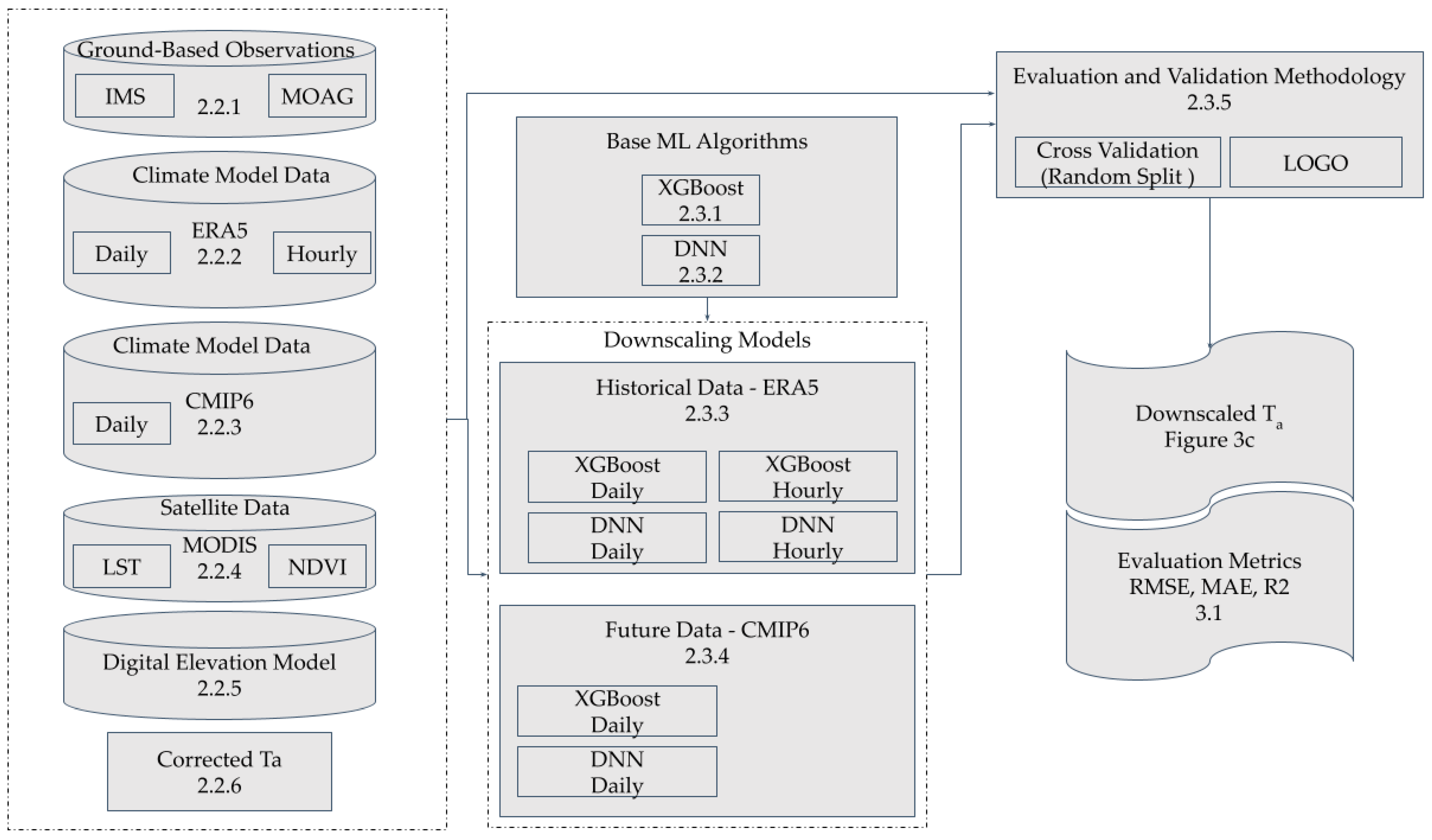
2. Data and Methods
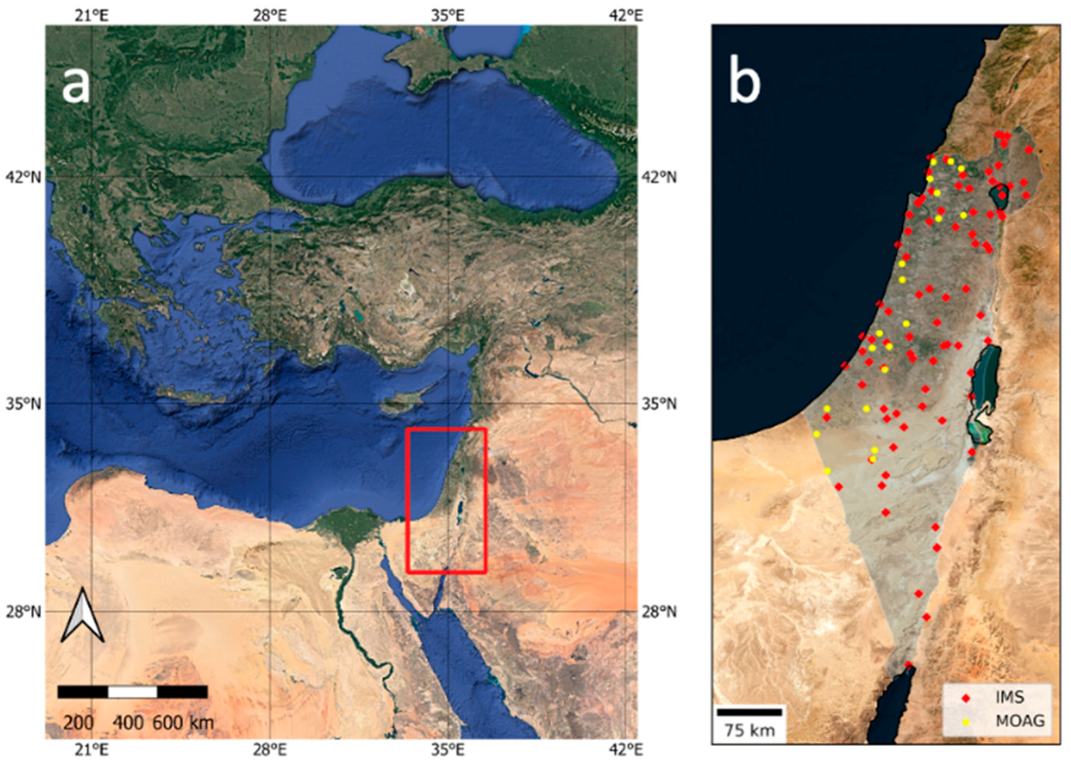
2.1. Study Area
2.2. Data


2.2.1. Ground-Based Observations
2.2.2. ERA5 Climate Model Data
2.2.3. CMIP6 Climate Model Data
2.2.4. MODIS Satellite Data
2.2.5. Digital Elevation Model Data
2.2.6. Corrected Ta Based on Height Difference and Adiabatic Lapse Rate
2.3. Methods
2.3.1. XGBoost Algorithm
2.3.2. Deep Neural Network
2.3.3. Models for Downscaling Historical Data
2.3.4. Models for Downscaling Future Data
2.3.5. Evaluation and Validation Methodology
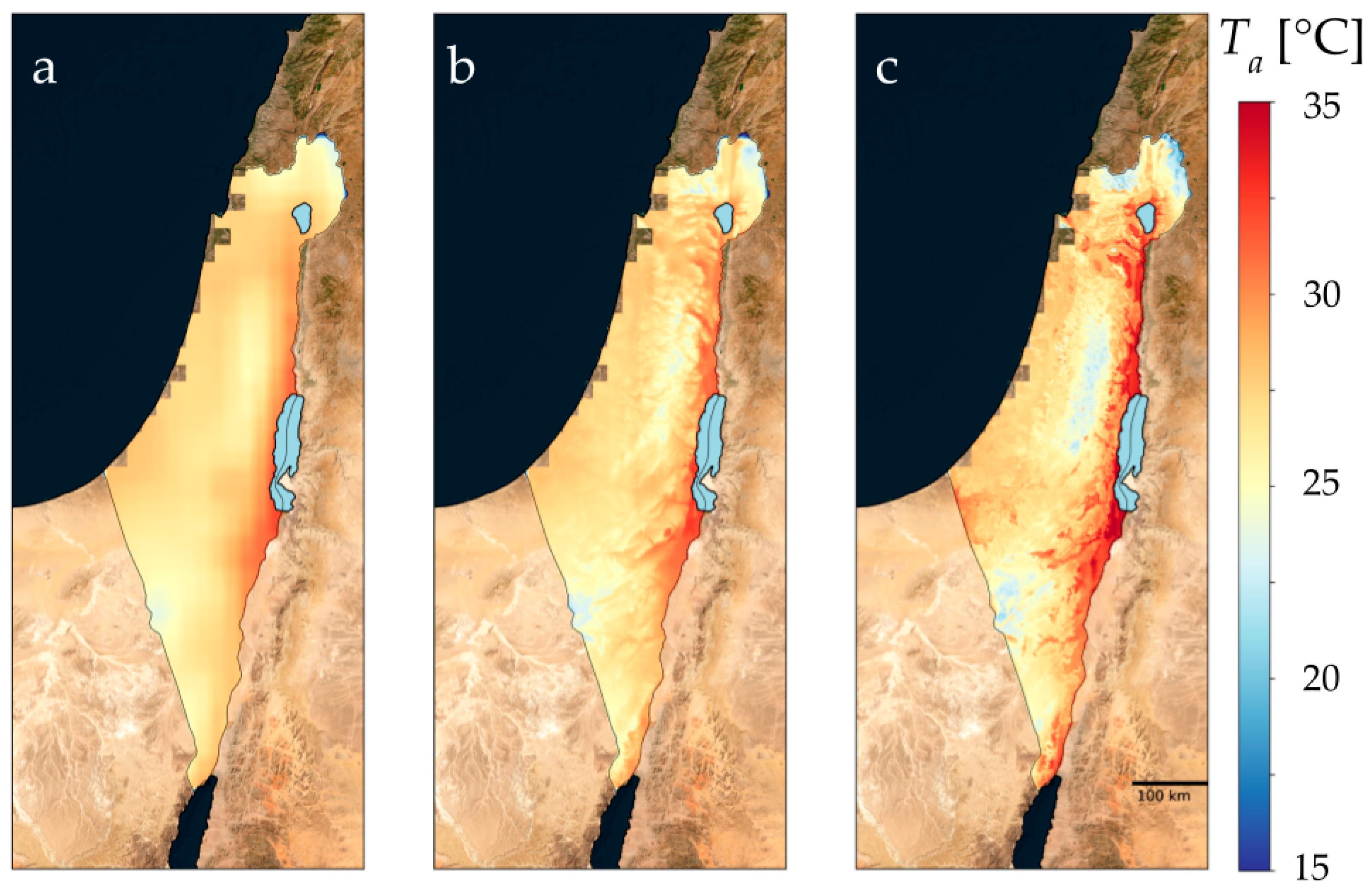
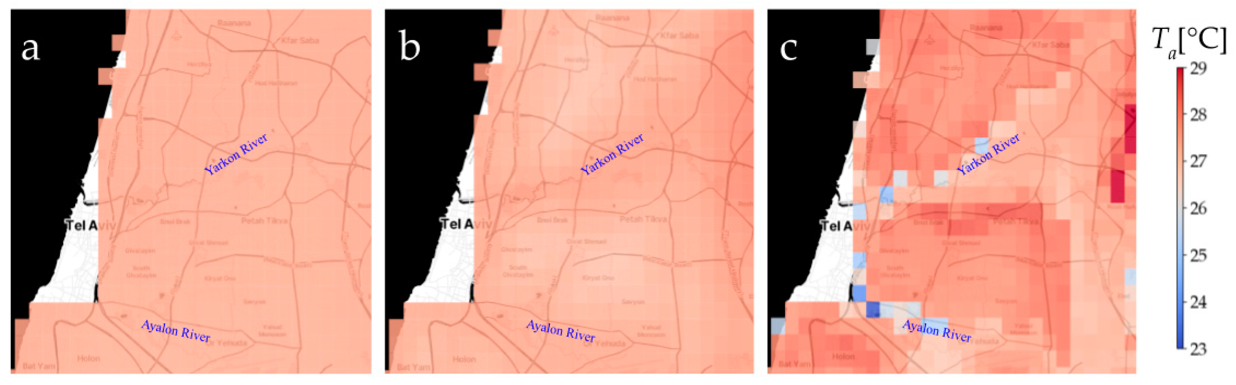
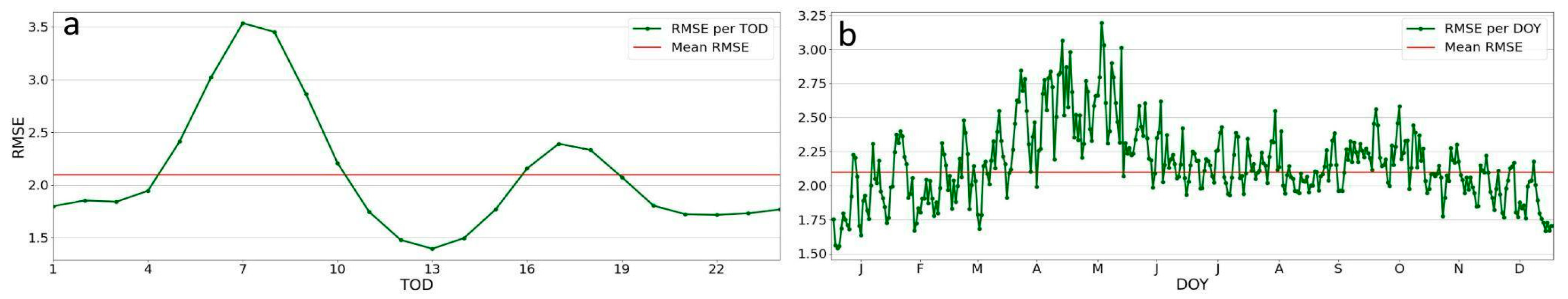
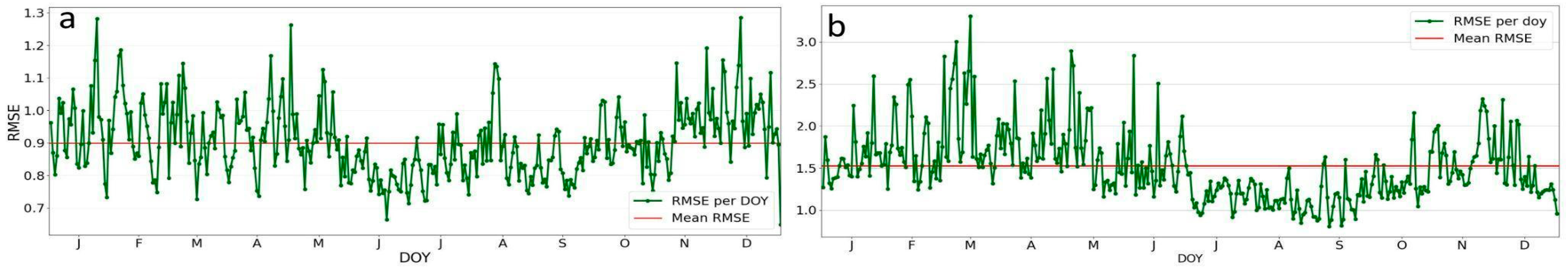
3. Results
3.1. Historical (ERA5) and Future (CMIP6) Data Models
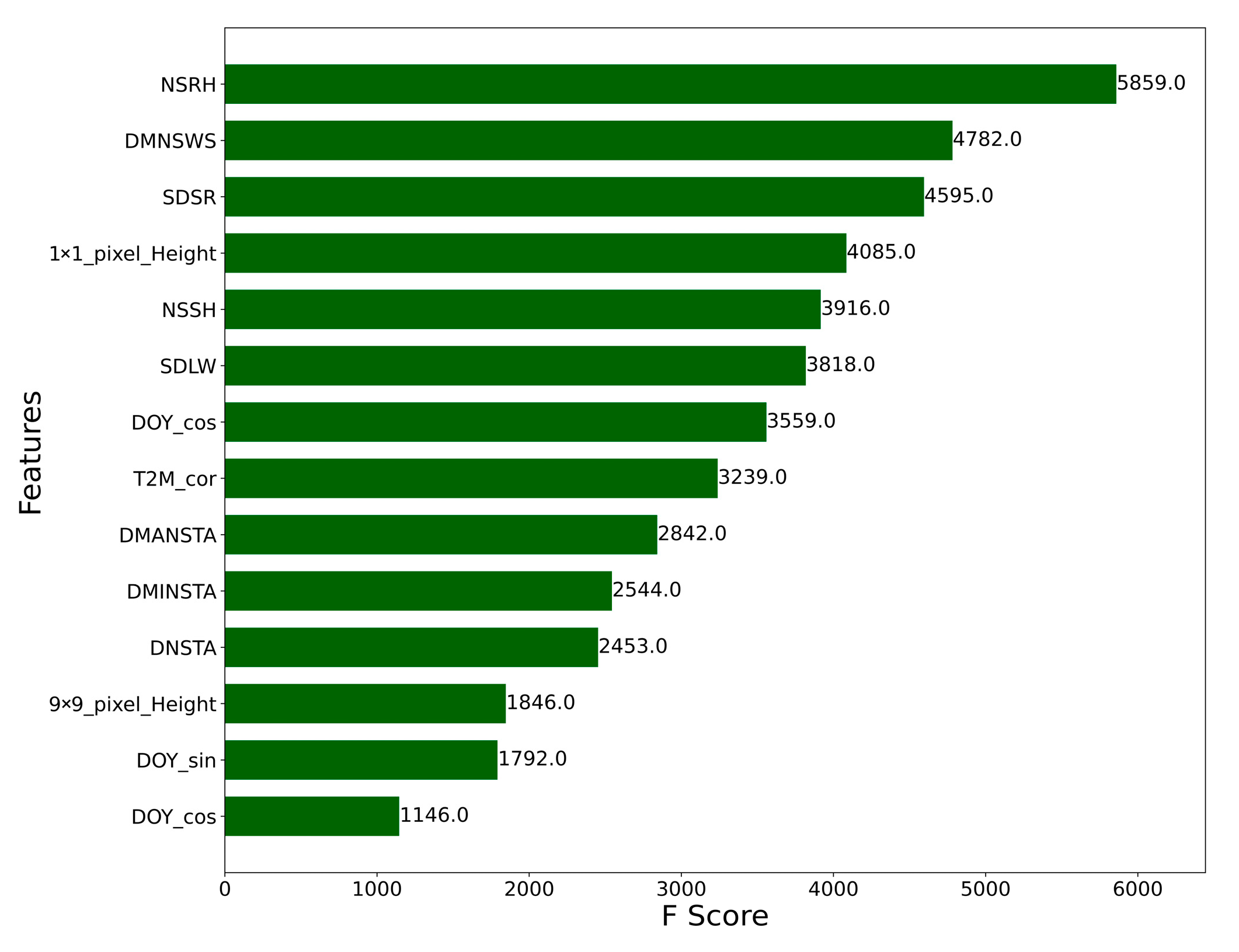
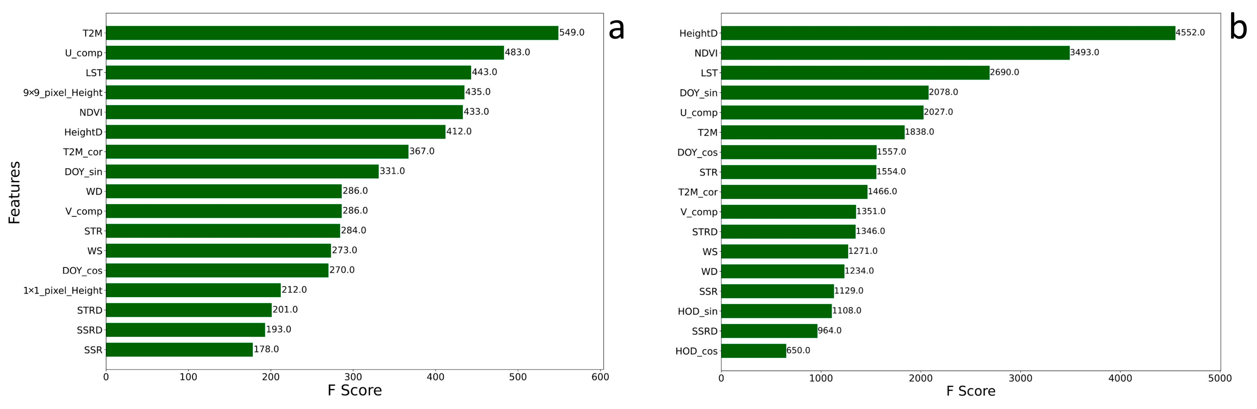
3.2. Feature Importance


4. Discussion
4.1. Results—Qualitative
4.2. Results—Quantitative
4.3. Methodology
5. Conclusions
Author Contributions
Funding
Data Availability Statement
Acknowledgments
Conflicts of Interest
References
- De Natale, F.; Alilla, R.; Parisse, B.; Nardi, P. A bibliometric analysis on drought and heat indices in agriculture. Agric. For. Meteorol. 2023, 341, 109626. [Google Scholar] [CrossRef]
- Li, D.; Nanseki, T.; Chomei, Y.; Kuang, J. A Review of Smart Agriculture and Production Practices in Japanese Large-Scale Rice Farming. J. Sci. Food Agric. 2022, 103, 1609–1620. [Google Scholar] [CrossRef] [PubMed]
- Dandrifosse, S.; Jago, A.; Huart, J.P.; Michaud, V.; Planchon, V.; Rosillon, D. Automatic quality control of weather data for timely decisions in agriculture. Smart Agric. Technol. 2024; in press. [Google Scholar] [CrossRef]
- Zhou, B.; Erell, E.; Hough, I.; Rosenblatt, J.; Just, A.C.; Novack, V.; Kloog, I. Estimating near-surface air temperature across Israel using a machine learning based hybrid approach. Int. J. Climatol. 2020, 40, 14. [Google Scholar] [CrossRef]
- Tsao, T.M.; Hwang, J.-S.; Chen, C.-Y.; Lin, S.-T.; Tsai, M.-J.; Su, T.-C. Urban climate and cardiovascular health: Focused on seasonal variation of urban temperature, relative humidity, and PM2.5 air pollution. Ecotoxicol. Environ. Safety 2023, 263, 115358. [Google Scholar] [CrossRef] [PubMed]
- Di Napoli, C.; Barnard, C.; Prudhomme, C.; Cloke, H.L.; Pappenberger, F. ERA5-HEAT: A global gridded historical dataset of human thermal comfort indices from climate reanalysis. Geosci. Data J. 2021, 8, 2–10. [Google Scholar] [CrossRef]
- Thrasher, B.; Wang, W.; Michaelis, A.; Melton, F.; Lee, T.; Nemani, R. NASA Global Daily Downscaled Projections, CMIP6. Sci. Data 2022, 9, 262. [Google Scholar] [CrossRef]
- Lensky, I.M.; Dayan, U.; Helman, D. Synoptic circulation impact on the near-surface temperature difference outweighs that of the seasonal signal in the Eastern Mediterranean. J. Geophys. Res. Atmos. 2018, 123, 11333–11347. [Google Scholar] [CrossRef]
- Lensky, I.M.; Dayan, U. Satellite observations of land surface temperature patterns induced by synoptic circulation. Int. J. Climatol. 2015, 35, 189–195. [Google Scholar] [CrossRef]
- Hemond, H.F.; Fechner, E.J. Chemical Fate and Transport in the Environment; Academic Press: Cambridge, MA, USA, 2022. [Google Scholar]
- Zhang, T.; Zhou, Y.; Zhao, K.; Zhu, Z.; Chen, G.; Hu, J.; Wang, L. A global dataset of daily maximum and minimum near-surface air temperature at 1 km resolution over land (2003–2020). Earth Syst. Sci. Data 2022, 14, 5637–5649. [Google Scholar] [CrossRef]
- Sebbar, B.-E.; Khabba, S.; Merlin, O.; Simonneaux, V.; El Hachimi, C.; Kharrou, M.H.; Chehbouni, A. Machine-Learning-Based Downscaling of Hourly ERA5-Land Air Temperature over Mountainous Regions. Atmosphere 2023, 14, 610. [Google Scholar] [CrossRef]
- Afshari, A.; Vogel, J.; Chockalingam, G. Statistical Downscaling of SEVIRI Land Surface Temperature to WRF Near-Surface Air Temperature Using a Deep Learning Model. Remote Sens. 2023, 15, 4447. [Google Scholar] [CrossRef]
- Mouatadid, S.; Easterbrook, S.; Erler, A.R. A Machine Learning Approach to Non-uniform Spatial Downscaling of Climate Variables. In Proceedings of the IEEE International Conference on Data Mining Workshops, ICDMW, New Orleans, LA, USA, 18–21 November 2017; pp. 332–341. [Google Scholar] [CrossRef]
- Karaman, Ç.H.; Akyürek, Z. Evaluation of near-surface air temperature reanalysis datasets and downscaling with machine learning based Random Forest method for complex terrain of Turkey. Adv. Space Res. 2023, 71, 5256–5281. [Google Scholar] [CrossRef]
- Arumugam, P.; Patel, N.R.; Kumar, V. Estimation of air temperature using the temperature/vegetation index approach over Andhra Pradesh and Karnataka. Environ. Earth Sci. 2022, 81, 79. [Google Scholar] [CrossRef]
- Lensky, I.M.; Dayan, U. Detection of Finescale Climatic Features from Satellites and Implications for Agricultural Planning. Bull. Amer. Meteor. Soc. 2011, 92, 1131–1136. [Google Scholar] [CrossRef]
- 10 & 1-Minutes Data (API). Israel Meteorological Service. Available online: https://ims.gov.il/en/ObservationDataAPI (accessed on 26 March 2023).
- Eyring, V.; Bony, S.; Meehl, G.A.; Senior, C.A.; Stevens, B.; Stouffer, R.J.; Taylor, K.E. Overview of the Coupled Model Intercomparison Project Phase 6 (CMIP6) experimental design and organization. Geosci. Model Dev. 2016, 9, 1937–1958. [Google Scholar] [CrossRef]
- Shiff, S.; Helman, D.; Lensky, I.M. Worldwide continuous gap-filled MODIS land surface temperature dataset. Sci. Data 2021, 8, 74. [Google Scholar] [CrossRef]
- Mo, Y.; Xu, Y.; Liu, Y.; Xin, Y.; Zhu, S. Comparison of gap-filling methods for producing all-weather daily remotely sensed near-surface air temperature. Remote Sens. Environ. 2023, 296, 113732. [Google Scholar] [CrossRef]
- Gorelick, N.; Hancher, M.; Dixon, M.; Ilyushchenko, S.; Thau, D.; Moore, R. Google Earth Engine: Planetary-scale geospatial analysis for everyone. Remote Sens. Environ. 2017, 202, 18–27. [Google Scholar] [CrossRef]
- Chakraborty, D.; Hazem, E. Advanced machine learning techniques for building performance simulation: A comparative analysis. J. Build. Perform. Simulation 2018, 12, 193–207. [Google Scholar] [CrossRef]
- Bitan, A.; Sa’Aroni, H. The horizontal and vertical extension of the Persian Gulf pressure trough. Int. J. Climatol. 1992, 12, 733–747. [Google Scholar] [CrossRef]


| Reference | Area | Methods * | RMSE (°C) | |
|---|---|---|---|---|
| Hourly | Daily | |||
| Sebbar 2023 [12] | Morocco (High Atlas) | MLR, SVR, XGB | 1.61 | |
| Afshari 2023 [13] | Germany (Urban) | CNN | 1.77 | |
| Zhou 2020 [4] | Israel | RF | 1.58 | |
| Mouatadid 2017 [14] | Canada | ANN (DL) | 0.85 | |
| Arumugam 2022 [16] | India | Linear regression | 1.09 | |
| Zhang 2022 [11] | Global | SVCM-SP | 1.75 | |
| Karaman 2023 [15] | Turkey | RF | 2.14 | |
| Feature Name | Short Name | Resolutions | Source | Historic/Future |
|---|---|---|---|---|
| Air temperature (2 m) | T2M | 10 km/h | ERA5 | Historic |
| Surface solar radiation downwards | SSRD | |||
| Surface thermal radiation downwards | STRD | |||
| Surface thermal radiation (net) | STRN | |||
| Surface solar radiation (net) | SSRN | |||
| U component | U_comp | |||
| V component | V_comp | |||
| Wind speed | WS | |||
| Wind direction | WD | |||
| Diff (ERA5—MODIS) mean pixel height | HeightD | 1 km/- | ||
| NDVI | NDVI | 250 m/day | MODIS AQUA | |
| LST | LST | 1 km/day | ||
| Day of Year | DOY | Both | ||
| Hour of Day | HOD | -/h | ||
| Corrected Ta (lapse rate) | T2M_cor | 1 km/h | ||
| Daily mean near-surface wind speed | DMNSWS | 27 km/day | CMIP6 | Future |
| Surface downwelling shortwave radiation | SDSR | |||
| Surface downwelling longwave radiation | SDLW | |||
| Near-surface specific humidity | NSSH | |||
| Near-surface relative humidity | NSRH | |||
| Daily Ta | DNSTA | |||
| Daily min Ta | DMINSTA | |||
| Daily max Ta | DMANSTA | |||
| Mean height in CMIP6 pixel | MHCP | 1 km/- | 90 m DEM | |
| Mean height in MODIS pixel | MHMP |
| (a) | |||||||||||||
| Climate Model/Baseline | Daily | Hourly | |||||||||||
| RMSE | MAE | R2 | RMSE | MAE | R2 | ||||||||
| Historic (ERA5) | Ta | 1.70 | 1.28 | 0.93 | 2.84 | 2.20 | 0.86 | ||||||
| Corrected Ta | 1.67 | 1.26 | 0.94 | 2.81 | 2.18 | 0.87 | |||||||
| Future (CMIP6) | Ta | 2.84 | 2.21 | 0.86 | - | ||||||||
| Corrected Ta | 2.81 | 2.18 | 0.87 | - | |||||||||
| (b) | |||||||||||||
| Climate Model/Algorithm | CV | LOGO | |||||||||||
| Daily | Hourly | Daily | Hourly | ||||||||||
| RMSE | MAE | R2 | RMSE | MAE | R2 | RMSE | MAE | R2 | RMSE | MAE | R2 | ||
| Historic (ERA5) | XGB | 0.79 | 0.58 | 0.99 | 1.39 | 1.00 | 0.97 | 1.50 | 1.55 | 0.95 | 2.77 | 2.14 | 0.87 |
| NN | 0.89 | 0.64 | 0.98 | 1.33 | 0.95 | 0.97 | 0.98 | 0.67 | 0.97 | 2.20 | 1.48 | 0.92 | |
| Future (CMIP6) | XGB | 1.24 | 0.88 | 0.96 | - | 2.14 | 1.62 | 0.88 | - | ||||
| NN | 1.34 | 0.98 | 0.95 | - | 1.86 | 1.30 | 0.91 | - | |||||
Disclaimer/Publisher’s Note: The statements, opinions and data contained in all publications are solely those of the individual author(s) and contributor(s) and not of MDPI and/or the editor(s). MDPI and/or the editor(s) disclaim responsibility for any injury to people or property resulting from any ideas, methods, instructions or products referred to in the content. |
© 2024 by the authors. Licensee MDPI, Basel, Switzerland. This article is an open access article distributed under the terms and conditions of the Creative Commons Attribution (CC BY) license (https://creativecommons.org/licenses/by/4.0/).
Share and Cite
Blizer, A.; Glickman, O.; Lensky, I.M. Comparing ML Methods for Downscaling Near-Surface Air Temperature over the Eastern Mediterranean. Remote Sens. 2024, 16, 1314. https://doi.org/10.3390/rs16081314
Blizer A, Glickman O, Lensky IM. Comparing ML Methods for Downscaling Near-Surface Air Temperature over the Eastern Mediterranean. Remote Sensing. 2024; 16(8):1314. https://doi.org/10.3390/rs16081314
Chicago/Turabian StyleBlizer, Amit, Oren Glickman, and Itamar M. Lensky. 2024. "Comparing ML Methods for Downscaling Near-Surface Air Temperature over the Eastern Mediterranean" Remote Sensing 16, no. 8: 1314. https://doi.org/10.3390/rs16081314
APA StyleBlizer, A., Glickman, O., & Lensky, I. M. (2024). Comparing ML Methods for Downscaling Near-Surface Air Temperature over the Eastern Mediterranean. Remote Sensing, 16(8), 1314. https://doi.org/10.3390/rs16081314