Georeferencing Strategies in Very Shallow Waters: A Novel GCPs Survey Approach for UCH Photogrammetric Documentation

Abstract

The growing interest of the scientific community in surveying and monitoring submerged assets is motivated by the increasing demand for high-resolution products with certified accuracies. While many instrumental and methodological solutions for documenting, monitoring, and studying archaeological and cultural heritage through geomatics techniques are already available for the terrestrial environment, the challenge remains open to the underwater context. High-resolution capability and accurate positioning are still difficult to achieve in these environments. This paper discusses the limitations of positioning and georeferencing techniques in the underwater environment. It explores how existing methods and new instruments can be used to perform accurate topographic surveys of ground control points (GCPs) in very shallow waters (within 5 m depths), which can support the photogrammetric reconstruction of underwater assets. This research presents two innovative prototypes: a self-built plastic marker for topographic use in the underwater environment and a self-built aluminum pole for topographic use in the marine environment. The prototypes are tested and validated with a tilt-compensating smart antenna to reduce planar and altimetric errors when the pole is not perfectly level and to work independently of the shore proximity required when using a total station to perform said measurements.

1. Introduction

Using photogrammetric techniques to document underwater cultural heritage (UCH) assets represents a crucial phase in their comprehensive study [1]. However, the efficacy of such documentation is contingent upon the implementation of robust georeferencing strategies for the accompanying topographic survey, ensuring consistency across all resultant products within a shared reference system [2]. Traditional archaeological excavation methodologies, particularly in underwater (UW) contexts, have often relied upon scale bars or approximate topographic measurements [3]. At the same time, scalebars are indispensable for providing accurate scales to generated 3D models and 2D products during photogrammetric recording [4,5]; their standalone usage results in a deficiency in absolute georeferentiation, a necessity for multitemporal documentation and data integration from diverse sources and instruments.

In contrast to terrestrial environments, where traditional topographic techniques are well-established, their direct applicability underwater is severely impeded [6]. A primary obstacle lies in the limited availability of satellite signals. Global Navigation Satellite Systems (GNSSs), including GPS, are significantly attenuated by water, rendering them impractical for positioning underwater assets [7]. Although topographic surveys employing side shot measures from total stations remain feasible near the shore and at shallow depths commensurate with the employed pole length, they necessitate an unobstructed line of sight between the total station and ground control points (GCPs) [8].

Recent years have witnessed advancements in underwater communication and positioning devices utilizing acoustic signals [9], albeit with accuracies primarily suited for navigational purposes rather than the precise localization of GCPs underwater. To address the challenge of underwater positioning, emerging methodologies propose the integration of pressure sensors for accurate scaling and leveling in underwater photogrammetry [10], alongside the installation of permanent GCPs to establish a robust reference frame for georeferencing and for evaluating the quality and accuracy of image blocks [11].

Recent advancements in underwater photogrammetry and 3D reconstruction techniques have significantly enhanced the documentation and analysis of submerged archaeological sites. Many authors commonly use photogrammetry in underwater archaeology and biology, from shallow water to deep water [2,12,13], demonstrating the efficacy of underwater photogrammetry in reconstructing underwater sites and showcasing its potential for detailed spatial documentation. IMCA’s (International Marine Contractors Association) guidance on subsea metrology [14] provides a comprehensive framework for ensuring accuracy and precision in underwater measurements crucial for archaeological surveys. Menna et al. [10] introduced a novel method incorporating pressure sensors for accurate scaling and leveling in underwater photogrammetry, addressing the challenges of variable water depths [15]. They proposed a structure from motion (SfM)-based approach tailored for documenting underwater pile fields, showcasing its effectiveness in archaeological science. Reich et al. [16] explored the precision potential of underwater networks for archaeological excavation, highlighting the synergistic application of trilateration and photogrammetry. Moreover, Wright et al. [17] conducted a comparative study between structure from motion photogrammetry and real-time kinematic survey methods, assessing the accuracy of underwater photogrammetry for archaeological purposes, further advancing our understanding of its capabilities and limitations.

Within archaeological topographic surveys, trilateration methodologies conducted via tape measures are commonplace, albeit prone to an average error of approximately 5 cm [2]. In very shallow water conditions, errors in reference point determination can be mitigated through total station side shot acquisitions from the shore, necessitating scuba diver operators to ensure the verticality of the prism. However, inherent limitations, including the influence of pole tilting angles and length, alongside meteorological and marine conditions, pose challenges to maintaining the required accuracy levels, underscoring the importance of implementing appropriate countermeasures for optimal results (Figure 1).

Due to the pole’s length and meteorological and marine conditions, handling it vertically is difficult. Employing this system without appropriate countermeasures will lead to weaker results than traditional trilateration.

The theoretical error on the measures is expressed in the Formula (1). It is mainly related to the planimetric component (2). In contrast, the vertical component (3), although still noticeable for longer poles and bigger tilt angles, is one level of magnitude smaller than the planimetric one (

Table 1. Theoretical planimetric error in the case of TS measurement of a prism for different pole lengths and different pole tilts whenever the pole is not perfectly perpendicular to the measured point.

Exy		Pole Length [m]
		2.00	2.50	3.00	3.50	4.00	4.50	5.00
Pole tilt [°]	0	0.000	0.000	0.000	0.000	0.000	0.000	0.000
	2	0.070	0.087	0.105	0.122	0.140	0.157	0.174
	4	0.140	0.174	0.209	0.244	0.279	0.314	0.349
	6	0.209	0.261	0.314	0.366	0.418	0.470	0.523
	8	0.278	0.348	0.418	0.487	0.557	0.626	0.696
	10	0.347	0.434	0.521	0.608	0.695	0.781	0.868

,

Table 2. Theoretical altimetric error is in the case of TS measurement of a prism for different pole lengths and different pole tilts whenever the pole is not perfectly perpendicular to the measured point.

Ez		Pole Length [m]
		2.00	2.50	3.00	3.50	4.00	4.50	5.00
Pole tilt [°]	0	0.000	0.000	0.000	0.000	0.000	0.000	0.000
	2	0.001	0.002	0.002	0.002	0.002	0.003	0.003
	4	0.005	0.006	0.007	0.009	0.010	0.011	0.012
	6	0.011	0.014	0.016	0.019	0.022	0.025	0.027
	8	0.019	0.024	0.029	0.034	0.039	0.044	0.049
	10	0.030	0.038	0.046	0.053	0.061	0.068	0.076

and

Table 3. Theoretical plano-planimetric error in the case of TS measurement of a prism for different pole lengths and different pole tilts whenever the pole is not perfectly perpendicular to the measured point.

E		Pole Length [m]
		2.00	2.50	3.00	3.50	4.00	4.50	5.00
Pole tilt [°]	0	0.000	0.000	0.000	0.000	0.000	0.000	0.000
	2	0.070	0.087	0.105	0.122	0.140	0.157	0.175
	4	0.140	0.174	0.209	0.244	0.279	0.314	0.349
	6	0.209	0.262	0.314	0.366	0.419	0.471	0.523
	8	0.279	0.349	0.419	0.488	0.558	0.628	0.698
	10	0.349	0.436	0.523	0.610	0.697	0.784	0.872

).

$$\mathrm{E}=\sqrt[2]{{{\mathrm{e}}_{\mathrm{x}\mathrm{y}}}^2+{{\mathrm{e}}_{\mathrm{z}}}^2}$$

(1)

$${\mathrm{e}}_{\mathrm{x}\mathrm{y}}=\mathrm{P}\sin \mathsf{\epsilon }$$

(2)

$${\mathrm{e}}_{\mathrm{z}}=\mathrm{P}(1-\cos \mathsf{\epsilon })$$

(3)

Furthermore, it is imperative to acknowledge the dynamic nature of the underwater environment, where factors such as water currents, turbidity, and tidal variations can further complicate the execution of precise topographic surveys. These environmental factors introduce additional sources of error, necessitating adaptive methodologies and robust calibration procedures to ensure the accuracy and reliability of georeferenced data collected in UW environments.

In light of these challenges, interdisciplinary collaborations between archaeologists, geomatics experts, and marine scientists are pivotal for developing innovative solutions and advancing state-of-the-art underwater photogrammetry and topographic surveying. Such collaborations foster the integration of diverse expertise and methodologies, refining techniques tailored specifically for the unique demands of documenting and preserving submerged cultural heritage.

The following chapters propose an easy-to-adopt and accurate method for the topographic measurement of reference points in very shallow water using GNSS equipment.

2. Materials and Methods

In the framework of this research, the possibility of measuring the coordinates of GCPs by using a GNSS N-RTK device (i.e., Leica GS18 or similar) when operating in very shallow water environments has been experimented with. For the specific UW use and given the need to adopt materials suitable for the marine environment, a 5 m aluminum pole was self-built (Section 2.1), together with a set of lightweight and portable set of conical markers (Section 2.2) that are described in the following paragraphs.

2.1. The 5 m Aluminum Pole (PALONE)

PALONE (Pole of ALuminum fOr mariNe Environment applications) is a self-built aluminum pole for topographic use in marine environment. Most topographic poles on the market do not reach the length of 5 m, which is a good length compromise when operating in very shallow water. Moreover, some 5 m length poles available on the market are telescopic; with this comes the disadvantage of having an undesired “fishing rod” effect (Figure 2) due to the reduced diameter of the last sections and due to the momentum generated by the mass attached to the end of the pole that, together with marine and environmental condition (wind and sea waves), might invalidate the measurement process. In addition, they require a fixed rather than movable bubble level because the operator will usually check the verticality of the pole at the water surface.

The PALONE self-built topographic pole is composed of 4 calibrated sections (Figure 3), which are connected by a plug-and-socket connection system (Figure 4) and secured together using a set of Inox fastening clips (Figure 5).

2.2. The Conic Underwater Marker (CONETTO)

CONETTO (CONical marker for undErwaTer Topographic Operations) is an underwater self-built plastic marker for topographic use (Figure 6).

The CONETTO device represents an advancement in underwater topographic materialization technology. It was specifically engineered to address the complex challenges inherent in accurately marking and surveying submerged environments, such as seabeds and lake floors.

The CONETTO device is designed as a multifunctional tool featuring a support portion and a conically shaped body. It is crafted to house a filling material that provides ballast upon deployment. The support portion boasts a dynamic design, featuring a customizable cover or cap that facilitates easy access for filling the device with ballast material. Meanwhile, with its polygonal or circular base, the conical body culminates in an apex that is the focal point for topographic referencing. This apex is crafted with a specialized fitting to seamlessly integrate with a topographic pole (Figure 7), ensuring precise alignment during survey operations.

One of the most remarkable features of the CONETTO device is its innovative anchoring mechanism, which leverages a robust anchoring element embedded within the support portion and body. This element, characterized by a rod-shaped configuration, exhibits exceptional grip strength when deployed in sandy or clayey substrates, enhancing stability and minimizing displacement. Additionally, a strategically implemented rough finish on select surfaces further augments friction with the seabed, bolstering overall anchorage (Figure 8).

Constructed from high-density materials, notably polyvinyl chloride (PVC), the CONETTO device boasts negative hydrostatic buoyancy, ensuring reliable submersion even in the most challenging marine environments. This buoyancy profile facilitates ease of deployment and mitigates the risk of unintentional displacement during operation.

The transformative impact of the CONETTO device is underscored by its unparalleled precision and accuracy. It achieves remarkable performance levels comparable to terrestrial survey methods utilizing advanced GNSS N-RTK techniques (Figure 9). With a root mean square error (RMSE) of approximately 2 cm, the CONETTO device sets a new standard for underwater surveying, enabling researchers and engineers to obtain unparalleled quality and reliable data.

Furthermore, the CONETTO device embodies a paradigm shift in terms of accessibility and affordability, with a design ethos centered on simplicity, sustainability, and mass producibility. Whether assembled through industrial manufacturing or artisanal craftsmanship, its constituent materials’ lightweight and recyclable nature ensures widespread availability and cost-effectiveness.

From its inception to real-world deployment, the CONETTO device represents an achievement of interdisciplinary innovation, seamlessly blending engineering, geomatics, and environmental conservation principles. The CONETTO device paves the way for transformative advancements in marine research, infrastructure development, and historic preservation by offering a versatile, user-friendly solution for underwater topographic materialization.

From Concept to Prototyping

The prototype of CONETTO has been self-built by assembling a plastic food container with a kitchen funnel; the funnel is riveted to the food box, and the corresponding inner circle is cut off from the plastic of the food container (Figure 10). This ensures the stackability and, therefore, the portability of the cones (Figure 11).

It can be used on rocky and sandy seabeds; it will be sufficient to fill it with sand or gravel retrieved directly on site before starting the survey; this will also be cost-efficient in case the cones have to be shipped or carried for long travels. For use in a sandy environment, it is possible to exploit an additional 40 mm length rod that can be inserted inside the cone and secured using bolts and nuts. An 8 mm column nut completes the top of the cone, allowing the easy placement of the pole tip.

2.3. Tilt Compensation Smart Antenna (Leica GS18 GNSS RTK Rover)

To reduce the plano-altimetric error introduced by TS measurements when the pole is not perfectly leveled (Figure 1) and to work independently from the shore proximity, it is possible to employ GNSS receivers that can compensate for the tilting errors; in the framework of this research, a Leica GS18 (Figure 12) has been employed (https://leica-geosystems.com/en-us/products/gnss-systems/smart-antennas/leica-gs18, accessed on 6 April 2024).

The device is provided with a tilting compensation option that can estimate and compensate the pole’s tilting angle via an accelerometer and the tilting direction using an IMU (this method is immune to magnetic disturbances that affect the tilting direction, like similar systems based on the compass) [18].

This will mitigate the systematic error introduced by the not-leveled pole, as an independent study has shown that the Leica GS18 can operate at tilt angles above 30° while maintaining a three-dimensional accuracy (3D CQ) of less than 20 mm [19].

It can be used in RTK with a base-rover configuration or with a Network-RTK (such as HxGN SmartNet—https://hxgnsmartnet.com/en-us/, accessed on 6 April 2024). However, it is important to consider that in the N-RTK mode, survey operators must ensure that the surveyed points are inside the network. Otherwise, the measurements will lack accuracy due to extrapolation outside the network. Whenever it is impossible to operate within the network boundaries, it is strongly advised to work in RTK mode, coupling another GNSS antenna via radio to be used as a base near the shore.

3. Results

The following paragraphs are related to the test and validation of the proposed solution: In Section 3.1, an assessment of the tilting compensated GNSS receiver has been performed by conducting a comparison with the Leica AP20 AutoPole, a new instrument by Hexagon Leica composed of a 360 Leica prism mounted on top of a 2.40 m (max) telescopic pole. The system provides a device that communicates the height of the pole to the TS. Moreover, it streams the tilt angle and direction to the TS for real-time compensation of the acquired topographic measures, which are performed by the automatic recognition, locking, and tracking of the 360 prisms. Section 3.2 discusses the accuracy of the GS18 mounted on the self-built pole by comparing a set of nine GCPs measured with both GNSS N-RTK tilt compensation antenna and TS. Another analysis is related to the stability of the conical markers over time, as they were measured again the day after to look for their stability, i.e., change of position on the seabed related to a strong current or other factors.

3.1. Assessment of the Tilting Compensation of the Leica GS18 and Comparison with the Leica AP20 AutoPole

This experiment analyzed the possible differences between a TS (Total Station) side shot acquisition (generally more accurate) and an N-RTK GNSS survey. According to the usual conditions in a water environment and the related problems in obtaining the verticality of a pole, tilt compensation is necessary to reduce the errors in the GCPs measurements. To find the more accurate system for measuring points in underwater environments, a comparison between the tilting systems embedded in the GNSS and in the Leica AutoPole was conducted. The test was conducted in a dry environment, measuring three known vertexes with the above devices using the approach reported below.

In detail, the experimental investigation delineated in this passage has been executed to juxtapose the precision achievable through the utilization of the Leica GS18 against that of the Leica AP20 AutoPole.

The genesis of the AP20 AutoPole can be traced back to the breakthroughs facilitated by the GS18 T smart antenna. This pioneering antenna surmounted the traditional limitations of GNSS poles, heralding a novel era of technological advancement conducive to seamless integration within the total station ecosystem. By amalgamating this innovative capacity with additional functionalities aimed at autonomously detecting fluctuations in pole height and obviating the need for manual calibration, the AP20 was conceptualized as a holistic solution to contemporary surveying challenges [20].

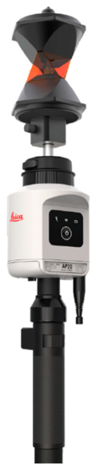
The AP20 AutoPole, as depicted in Figure 13, represents a paradigm shift in surveying instrumentation engineered by Hexagon Leica. Comprising a 360-degree Leica prism atop a telescopic pole capable of extending up to 2.40 m, this system embodies a sophisticated apparatus designed to communicate precise positional data to the TS. Furthermore, it facilitates real-time data transmission regarding the pole’s tilt angle and orientation, thereby enabling dynamic compensation of acquired topographic measurements. This is achieved through the automated recognition, fixation, and continual tracking of the 360-degree prism, ensuring unparalleled accuracy and efficiency in surveying endeavors.

The entirety of the measurement framework operates on the foundation of dependable sensor inputs, circumventing the reliance on manual leveling constraints. Embedded within the AP20 is Inertial Measurement Unit (IMU) technology, which serves to ascertain the three-dimensional alignment of the pole within its spatial context. Analogous to the sophisticated design of the Leica GS18 T [18], the IMU employed within the AP20 is predicated upon industrial-grade Microelectromechanical Systems (MEMSs), housing a triad of sensors, a three-axis accelerometer and a three-axis gyroscope, meticulously calibrated to capture acceleration and angular velocity with utmost precision.

In conjunction with the total station’s continuous tracking of target positions, these sensor readings are seamlessly integrated into a bespoke Inertial Navigation System (INS) meticulously integrated within the AP20 apparatus. The INS algorithm, employing rigorous mathematical computations, orchestrates the transformation and fusion of IMU-derived measurements into the total station’s coordinate system, thereby discerning the spatial orientation of the pole and its attendant quality metrics with unparalleled accuracy [20].

The test has been carried out by following the steps below:

• Identifying a set of points (A, B, and C) of known coordinates.
• Each point is measured a dozen times with the following:
  • Three configurations:
    • The pole is tilted but steady.
    • Pole tilts simulating operative conditions in water (maximum five gons).
    • Pole tilts simulating operative conditions in water (max ten gons).
  • Three instrument settings:
    • AP20 tilt compensation ON
    • GS18 (N-RKT) tilt compensation ON single epoch.
    • GS18 (N-RTK) tilt compensation ON 10 s acquisition.

The test aimed to assess the standard deviations and coordinate residuals for each point (A, B, and C) across three distinct instrument settings and configurations, replicating operational scenarios typical of underwater (UW) surveying.

The comprehensive findings of the test are elucidated in the subsequent tables (Table 4, Table 5 and Table 6) and visual representations (Figure 14, Figure 15, Figure 16, Figure 17, Figure 18, Figure 19, Figure 20, Figure 21 and Figure 22).

Table 4. Standard deviations of the measurements of point A coordinates, with AP20 and GS18 (single epoch and 10 s acquisition) in steady and tilting configurations (max five gons and max ten gons).

Test Type	Instrument	σx [m]	σy [m]	σz [m]
Steady	AP20	0.002	0.003	0.002
	GS18	0.007	0.011	0.020
	GS18 (10 s)	0.005	0.015	0.020
Tilt max five gons	AP20	0.002	0.001	0.000
	GS18	0.004	0.003	0.008
	GS18 (10 s)	0.005	0.005	0.007
Tilt max ten gons	AP20	0.003	0.005	0.001
	GS18	0.004	0.005	0.013
	GS18 (10 s)	0.007	0.008	0.010

Table 4. Standard deviations of the measurements of point A coordinates, with AP20 and GS18 (single epoch and 10 s acquisition) in steady and tilting configurations (max five gons and max ten gons).

Test Type	Instrument	σx [m]	σy [m]	σz [m]
Steady	AP20	0.002	0.003	0.002
	GS18	0.007	0.011	0.020
	GS18 (10 s)	0.005	0.015	0.020
Tilt max five gons	AP20	0.002	0.001	0.000
	GS18	0.004	0.003	0.008
	GS18 (10 s)	0.005	0.005	0.007
Tilt max ten gons	AP20	0.003	0.005	0.001
	GS18	0.004	0.005	0.013
	GS18 (10 s)	0.007	0.008	0.010

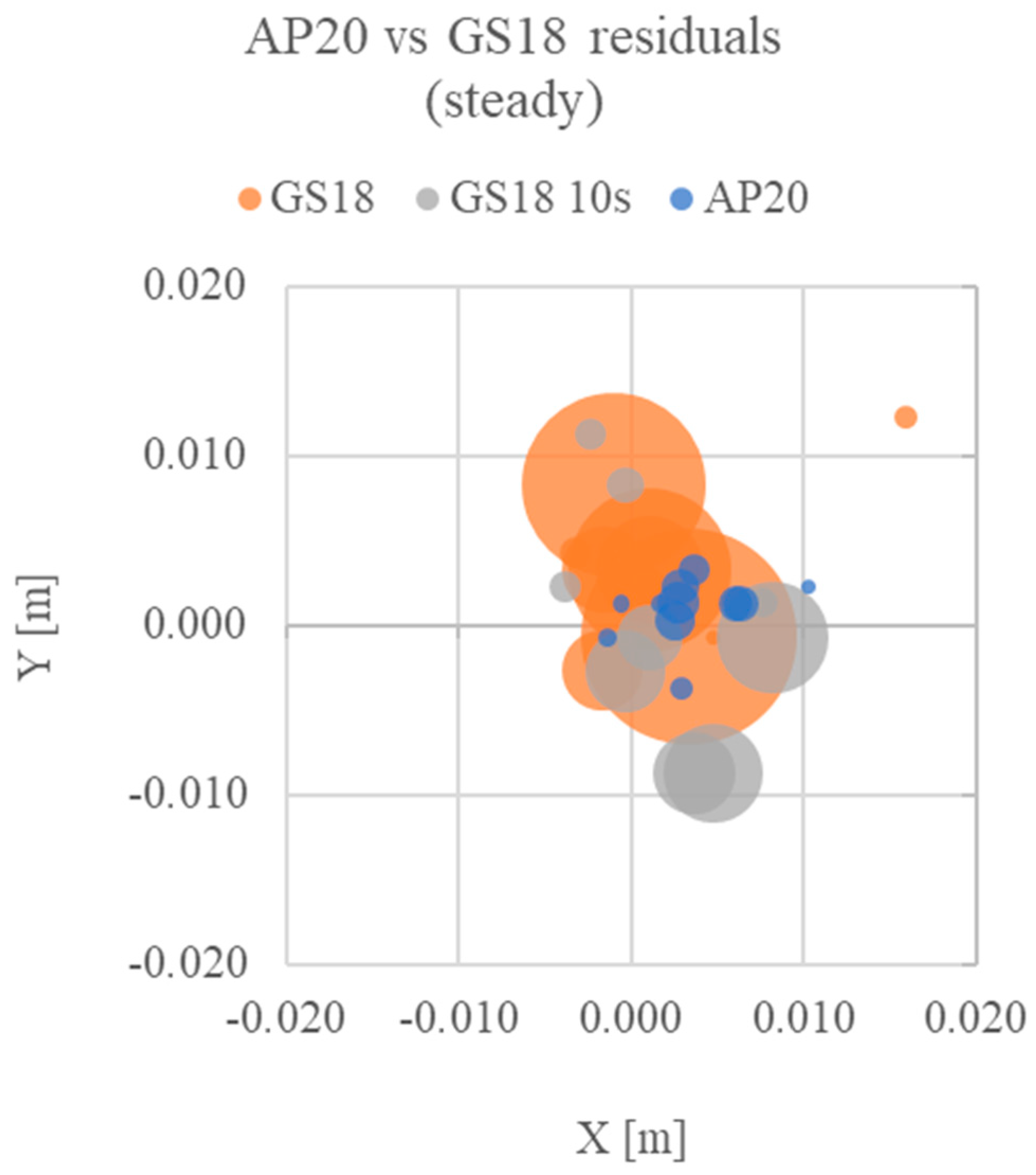
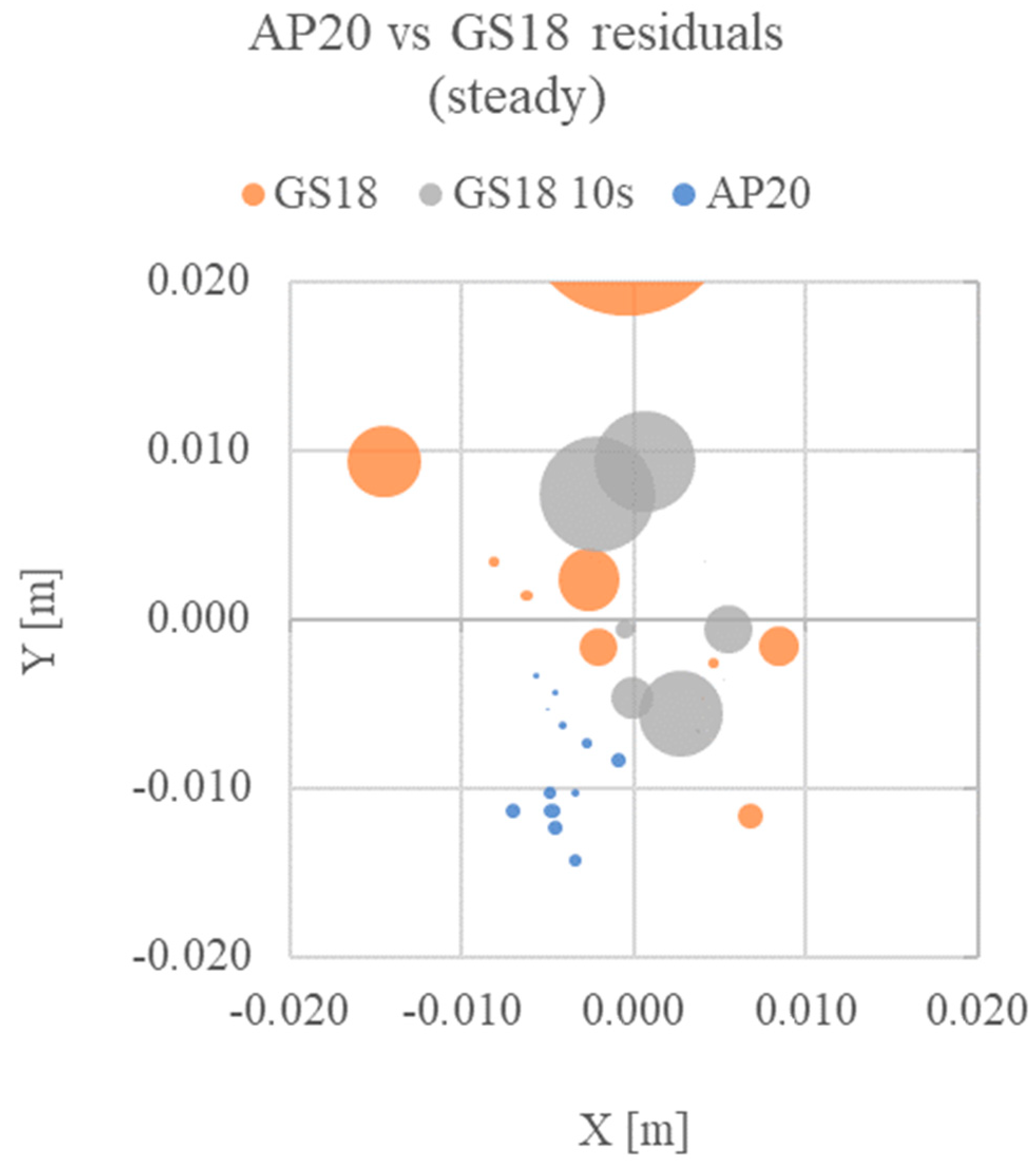
Figure 14. Relative coordinates plot for point A (0;0) for the test in steady configuration. X and Y are the planimetric residuals, while the point’s radius indicates the altimetric residual for each set of measures.

Figure 14. Relative coordinates plot for point A (0;0) for the test in steady configuration. X and Y are the planimetric residuals, while the point’s radius indicates the altimetric residual for each set of measures.

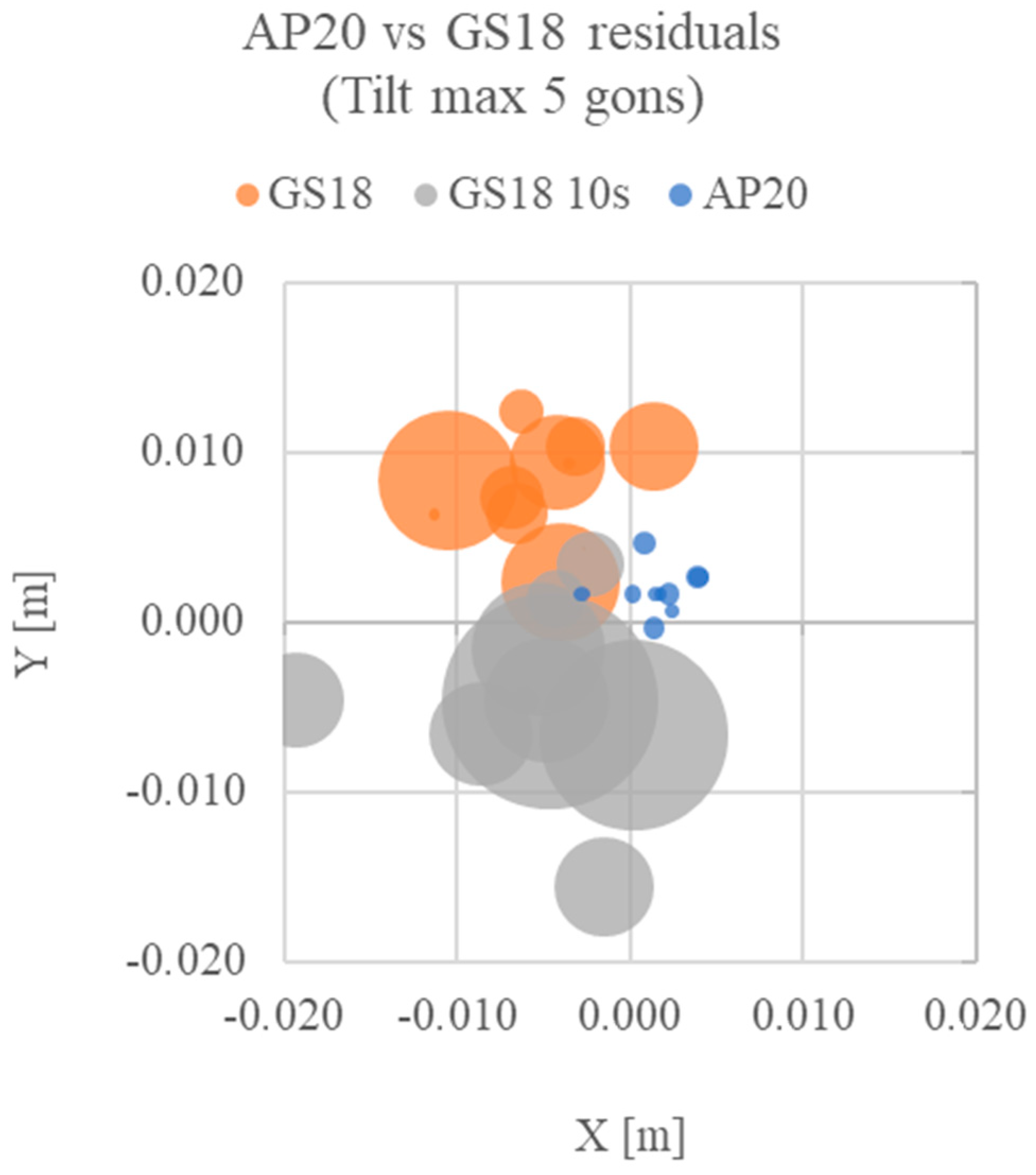
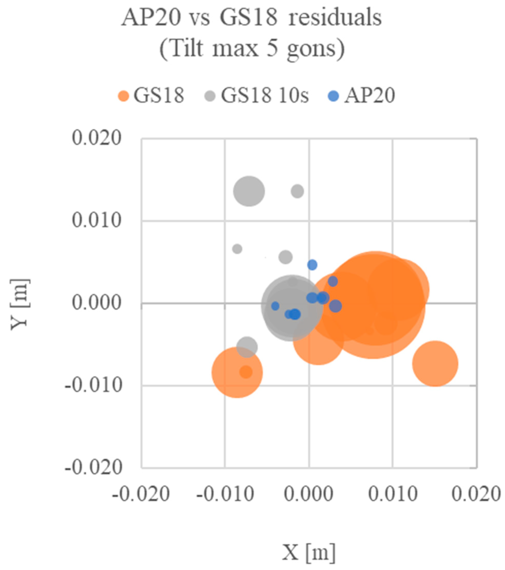
Figure 15. Relative coordinates plot for point A (0;0) for the test in tilting (max five gons) configuration. X and Y are the planimetric residuals, while the point’s radius indicates the altimetric residual for each set of measures.

Figure 15. Relative coordinates plot for point A (0;0) for the test in tilting (max five gons) configuration. X and Y are the planimetric residuals, while the point’s radius indicates the altimetric residual for each set of measures.

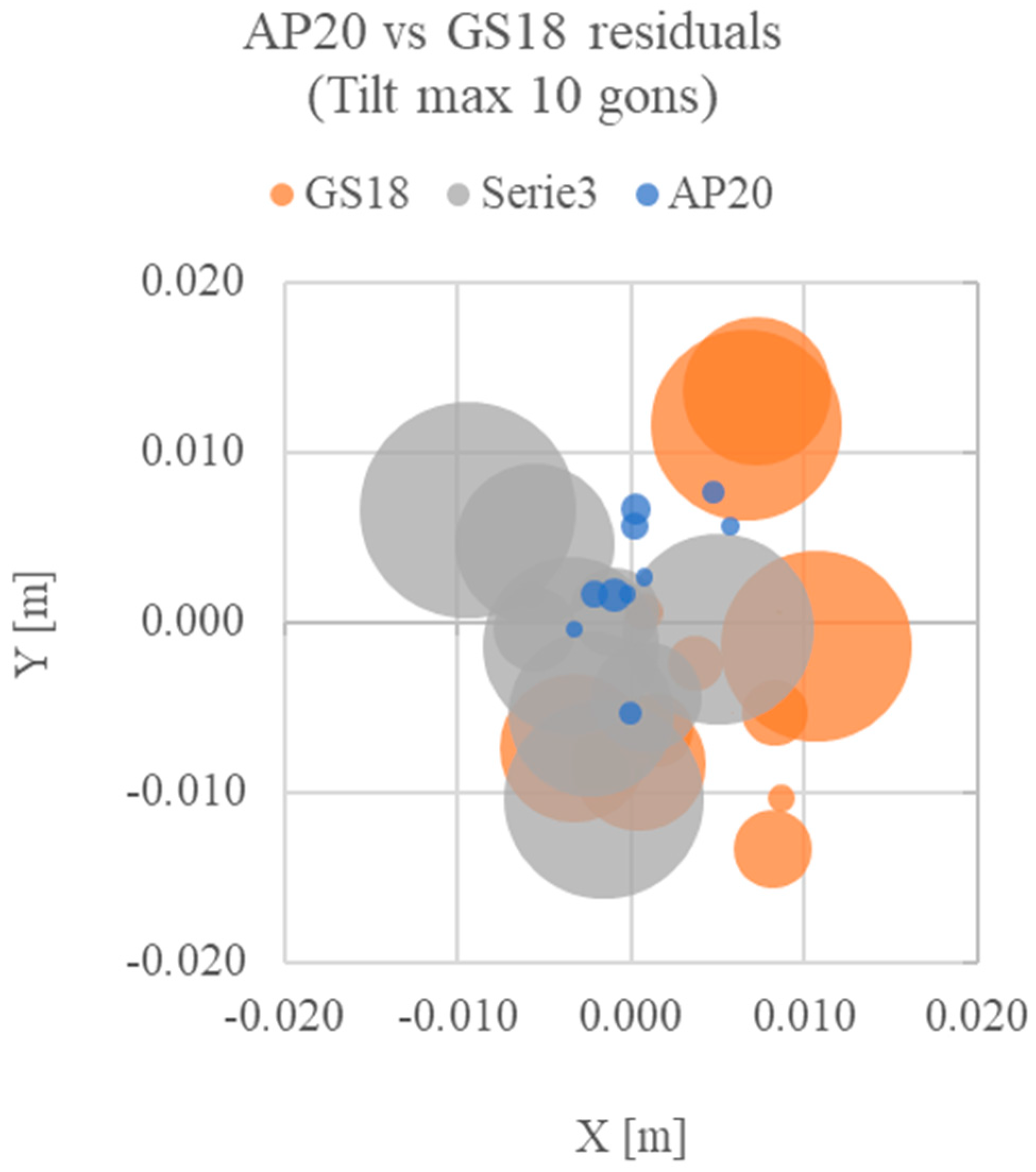
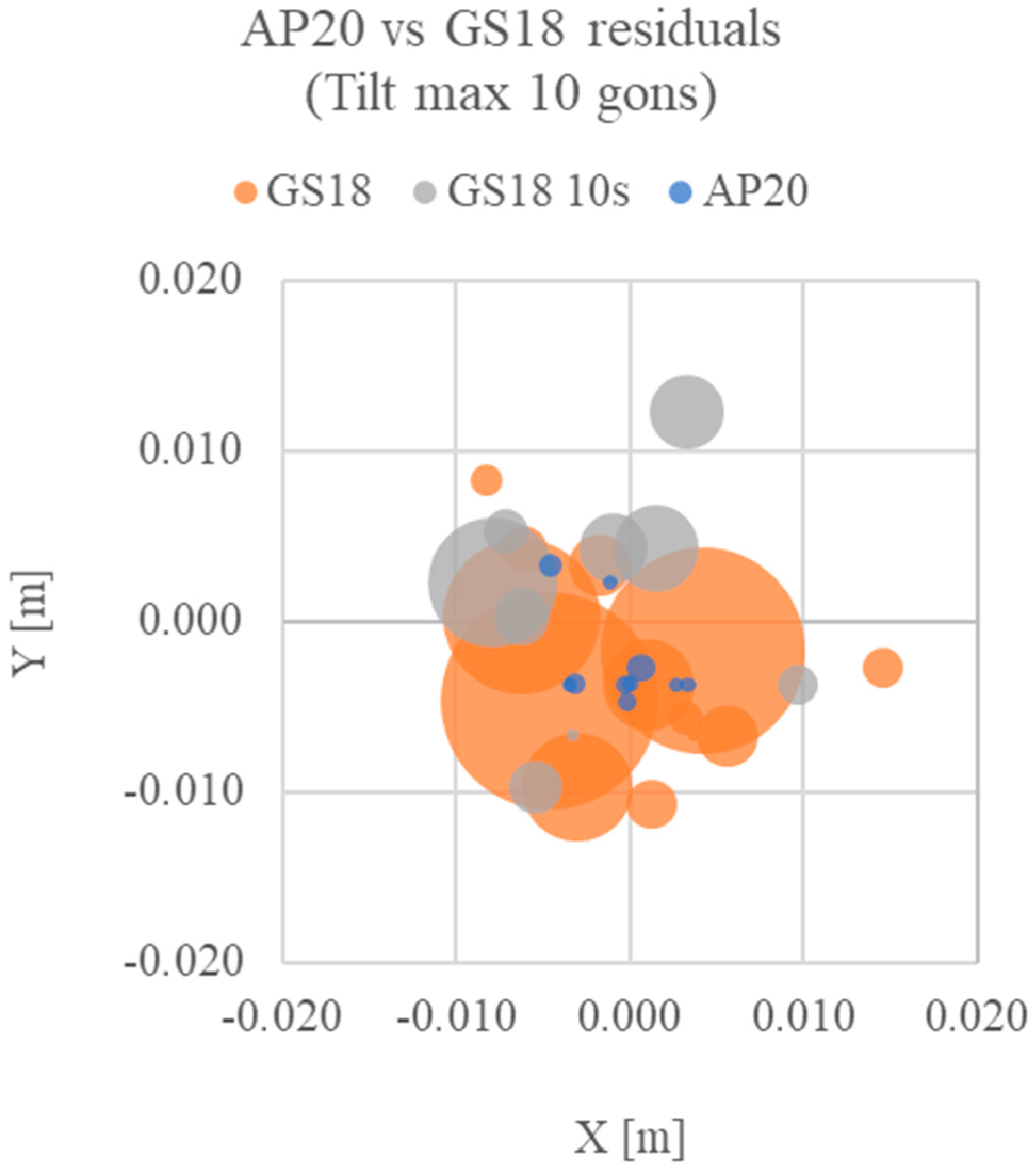
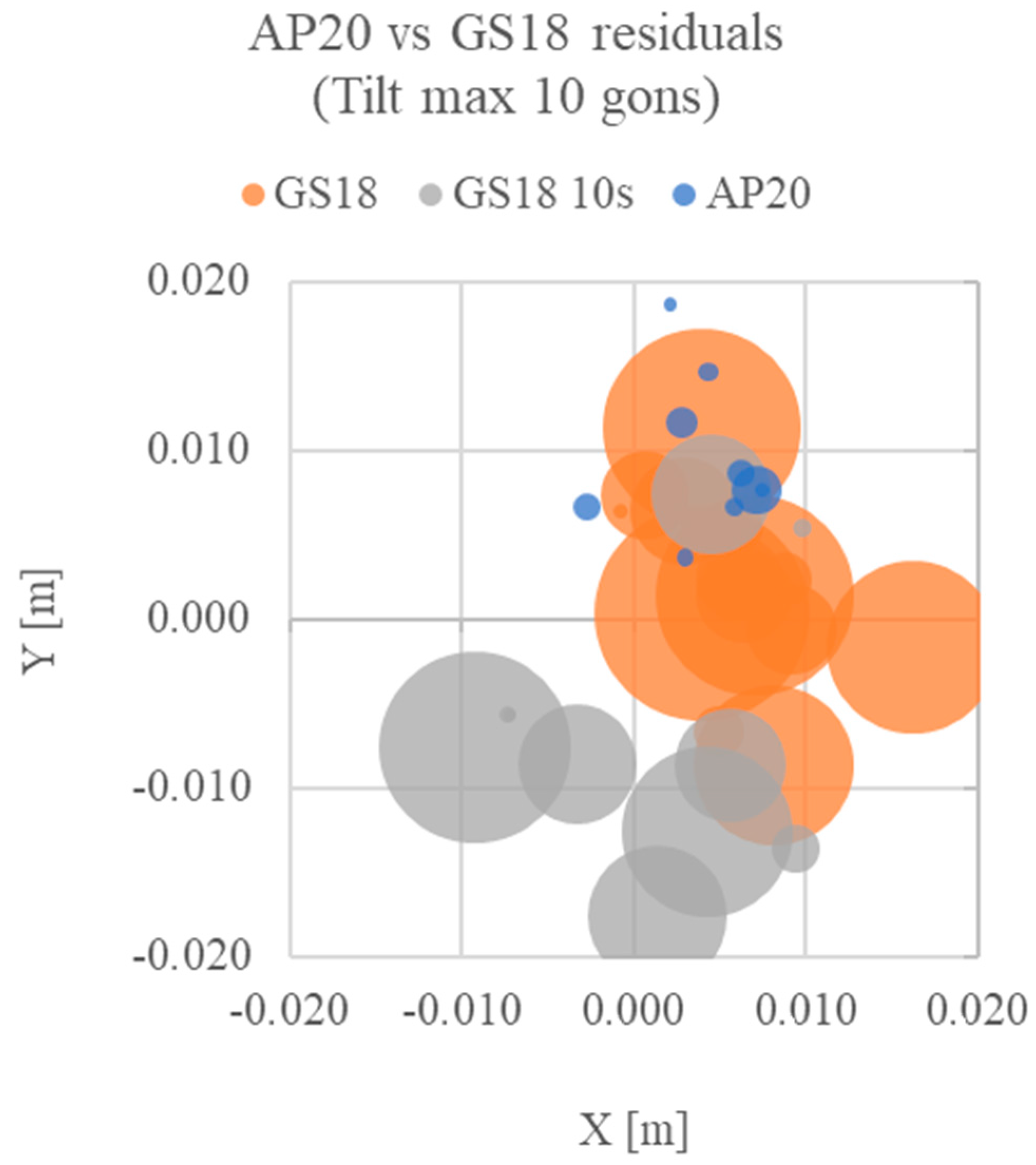
Figure 16. Relative coordinates plot for point A (0;0) for the tilting (max ten gons) configuration test. X and Y are the planimetric residuals, while the point’s radius indicates the altimetric residual for each set of measures.

Figure 16. Relative coordinates plot for point A (0;0) for the tilting (max ten gons) configuration test. X and Y are the planimetric residuals, while the point’s radius indicates the altimetric residual for each set of measures.

Table 5. Standard deviations of the measurements of point B coordinates, with AP20 and GS18 (single epoch and 10 s acquisition) in steady and tilting configurations (max five gons and max ten gons).

Test Type	Instrument	σx [m]	σy [m]	σz [m]
Steady	AP20	0.003	0.004	0.001
	GS18	0.003	0.004	0.006
	GS18 (10 s)	0.005	0.006	0.005
Tilt max five gons	AP20	0.003	0.004	0.001
	GS18	0.007	0.004	0.008
	GS18 (10 s)	0.003	0.006	0.005
Tilt max ten gons	AP20	0.002	0.002	0.000
	GS18	0.004	0.008	0.005
	GS18 (10 s)	0.004	0.005	0.005

Table 5. Standard deviations of the measurements of point B coordinates, with AP20 and GS18 (single epoch and 10 s acquisition) in steady and tilting configurations (max five gons and max ten gons).

Test Type	Instrument	σx [m]	σy [m]	σz [m]
Steady	AP20	0.003	0.004	0.001
	GS18	0.003	0.004	0.006
	GS18 (10 s)	0.005	0.006	0.005
Tilt max five gons	AP20	0.003	0.004	0.001
	GS18	0.007	0.004	0.008
	GS18 (10 s)	0.003	0.006	0.005
Tilt max ten gons	AP20	0.002	0.002	0.000
	GS18	0.004	0.008	0.005
	GS18 (10 s)	0.004	0.005	0.005

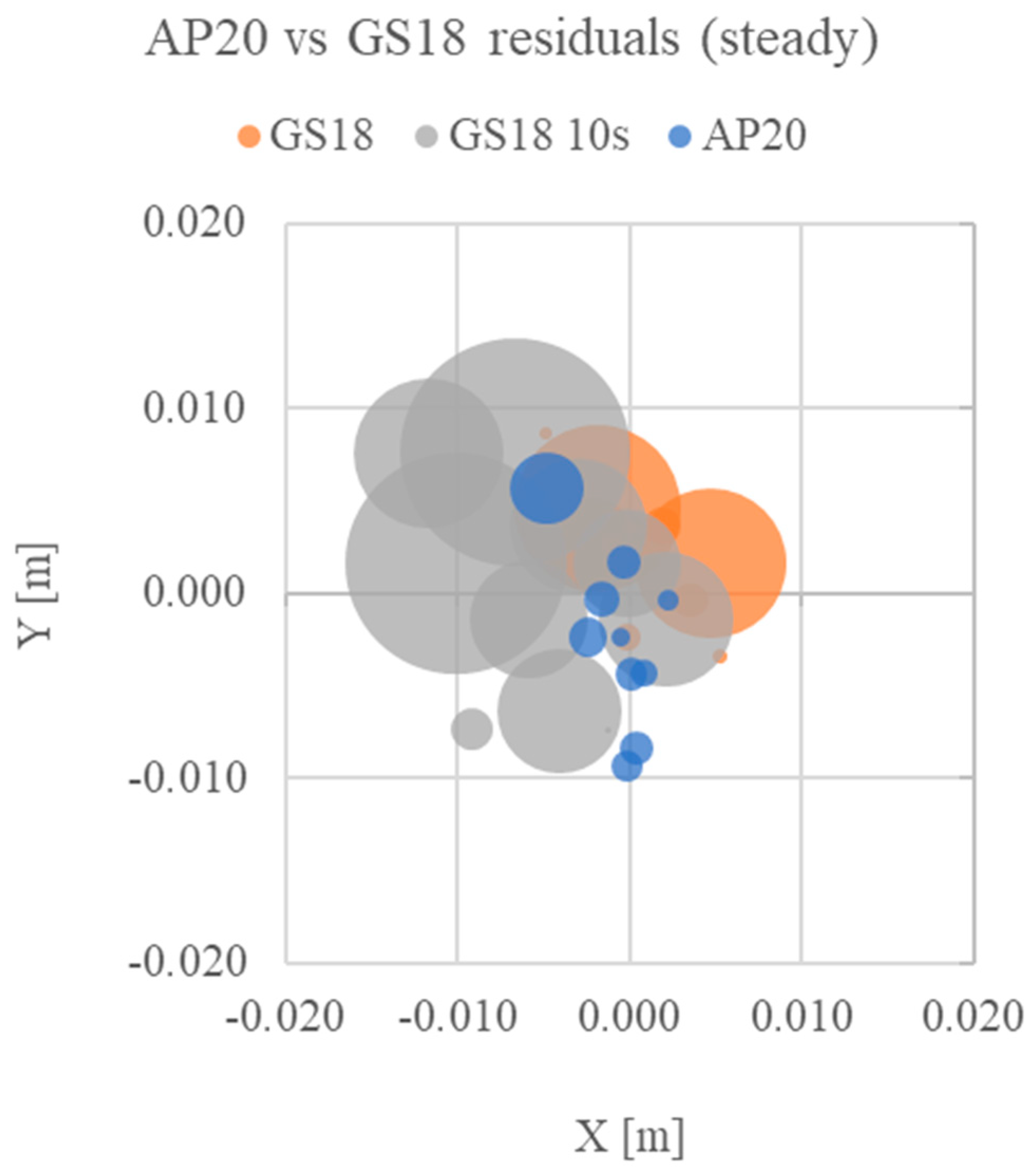
Figure 17. Relative coordinates plot for point B (0;0) for the test in steady configuration. X and Y are the planimetric residuals, while the point’s radius indicates the altimetric residual for each set of measures.

Figure 17. Relative coordinates plot for point B (0;0) for the test in steady configuration. X and Y are the planimetric residuals, while the point’s radius indicates the altimetric residual for each set of measures.

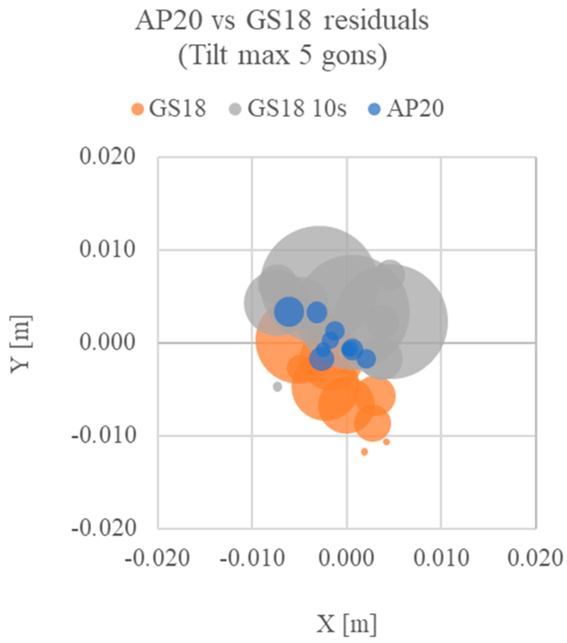
Figure 18. Relative coordinates plot for point B (0;0) for the tilting (max five gons) configuration test. X and Y are the planimetric residuals, while the point’s radius indicates the altimetric residual for each set of measures.

Figure 18. Relative coordinates plot for point B (0;0) for the tilting (max five gons) configuration test. X and Y are the planimetric residuals, while the point’s radius indicates the altimetric residual for each set of measures.

Figure 19. Relative coordinates plot for point B (0;0) for the tilting (max ten gons) configuration test. X and Y are the planimetric residuals, while the point’s radius indicates the altimetric residual for each set of measures.

Figure 19. Relative coordinates plot for point B (0;0) for the tilting (max ten gons) configuration test. X and Y are the planimetric residuals, while the point’s radius indicates the altimetric residual for each set of measures.

Table 6. Standard deviations of the measurements of point C coordinates, with AP20 and GS18 (single epoch and 10 s acquisition) in steady and tilting configurations (max five gons and max ten gons).

Test Type	Instrument	σx [m]	σy [m]	σz [m]
Steady	AP20	0.004	0.002	0.001
	GS18	0.005	0.004	0.007
	GS18 (10 s)	0.004	0.007	0.005
Tilt max five gons	AP20	0.004	0.002	0.001
	GS18	0.004	0.005	0.005
	GS18 (10 s)	0.005	0.004	0.006
Tilt max ten gons	AP20	0.002	0.003	0.001
	GS18	0.006	0.006	0.010
	GS18 (10 s)	0.005	0.006	0.006

Table 6. Standard deviations of the measurements of point C coordinates, with AP20 and GS18 (single epoch and 10 s acquisition) in steady and tilting configurations (max five gons and max ten gons).

Test Type	Instrument	σx [m]	σy [m]	σz [m]
Steady	AP20	0.004	0.002	0.001
	GS18	0.005	0.004	0.007
	GS18 (10 s)	0.004	0.007	0.005
Tilt max five gons	AP20	0.004	0.002	0.001
	GS18	0.004	0.005	0.005
	GS18 (10 s)	0.005	0.004	0.006
Tilt max ten gons	AP20	0.002	0.003	0.001
	GS18	0.006	0.006	0.010
	GS18 (10 s)	0.005	0.006	0.006

Figure 20. Relative coordinates plot for point C (0;0) for the test in steady configuration. X and Y are the planimetric residuals, while the point’s radius indicates the altimetric residual for each set of measures.

Figure 20. Relative coordinates plot for point C (0;0) for the test in steady configuration. X and Y are the planimetric residuals, while the point’s radius indicates the altimetric residual for each set of measures.

Figure 21. Relative coordinates plot for point C (0;0) for the tilting (max five gons) configuration test. X and Y are the planimetric residuals, while the point’s radius indicates the altimetric residual for each set of measures.

Figure 21. Relative coordinates plot for point C (0;0) for the tilting (max five gons) configuration test. X and Y are the planimetric residuals, while the point’s radius indicates the altimetric residual for each set of measures.

Figure 22. Relative coordinates plot for point C (0;0) for the tilting (max ten gons) configuration test. X and Y are the planimetric residuals, while the point’s radius indicates the altimetric residual for each set of measures.

Figure 22. Relative coordinates plot for point C (0;0) for the tilting (max ten gons) configuration test. X and Y are the planimetric residuals, while the point’s radius indicates the altimetric residual for each set of measures.

Upon analysis, it is evident that for AP20 measurements, consistency is maintained across all three points and configurations, with results exhibiting comparable standard deviations and coordinate residuals.

In contrast, when examining GS18 measurements, the steady configuration’s superiority becomes apparent in measurement accuracy. This configuration yields lower standard deviations and residuals, indicating heightened accuracy and reduced dispersion. However, the 10 s acquisition setting notably enhances accuracy solely in the z component.

Overall, the acquired results are highly promising, surpassing both conventional techniques and analog land surveying methodologies in terms of precision and reliability.

3.2. Accuracy Comparison with Total Station and Stability of the Markers over Time

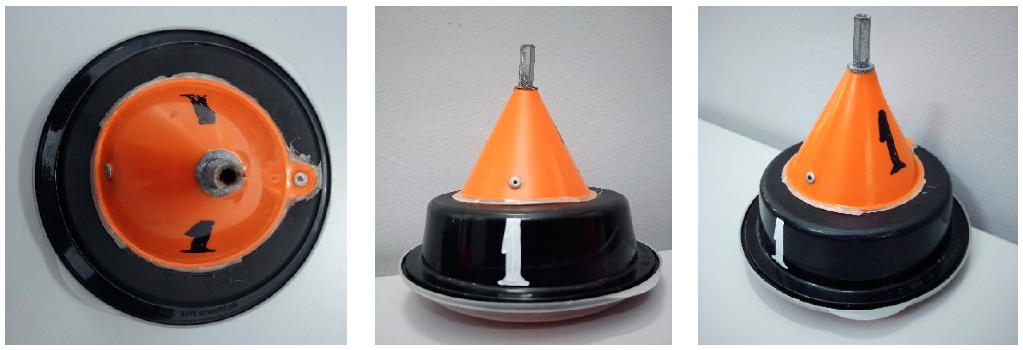
The analyses carried out are related to the stability of conical markers over time; the purpose of the validation is to measure the coordinates of the markers after their positioning on the seabed and in the following 24 h to analyze (if any) even minimal displacements related to bottom currents or other factors such as, for example, disturbance due to local flora and fauna or other external factors (boats or swimmers not foreseen in the survey operations). The test described was conducted in 2022 in Coluccia, north of Sardinia. In this context, the CONETTO system was tested for the first time in the relevant environment.

The procedure consisted of the following steps:

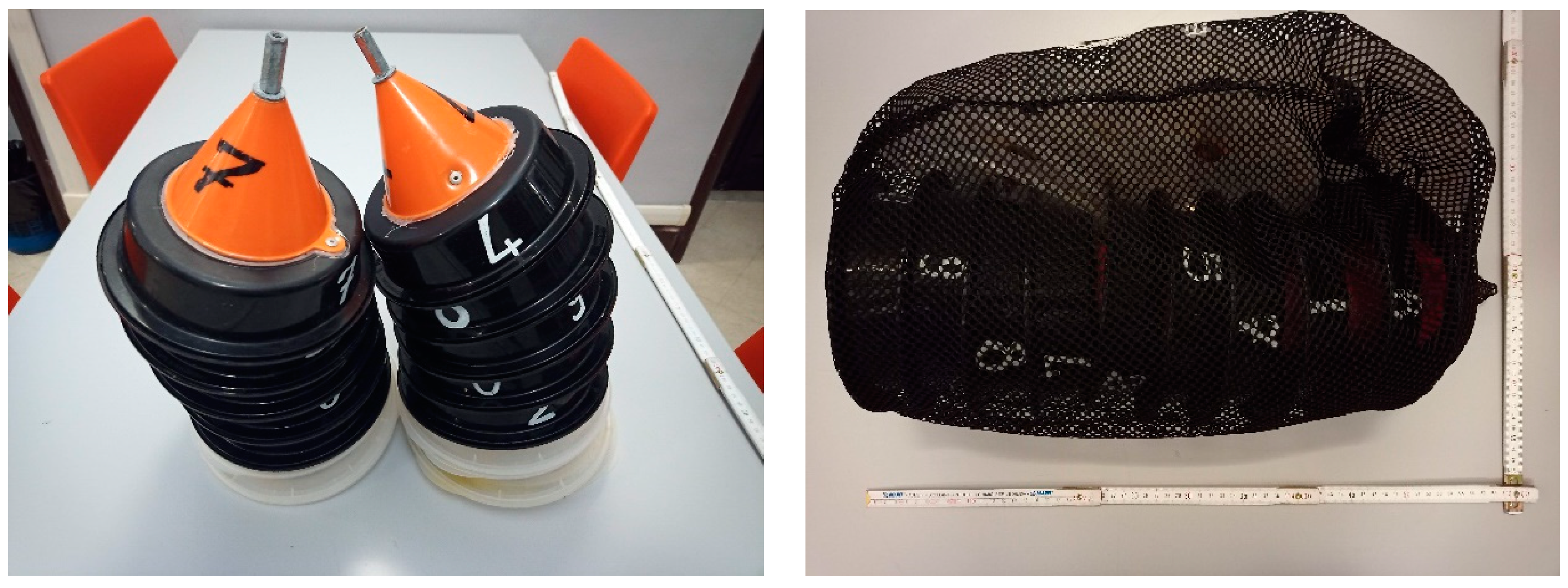
• A set of nine conical markers is placed within the survey area
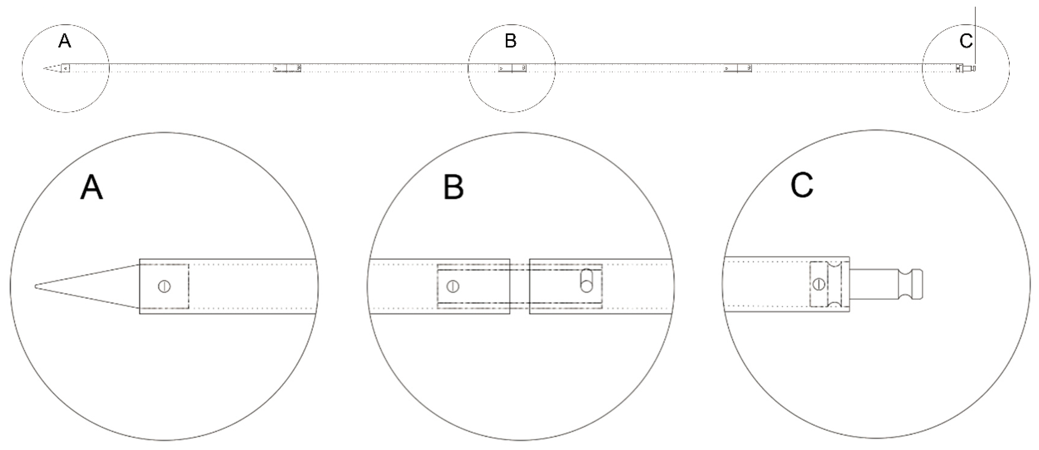
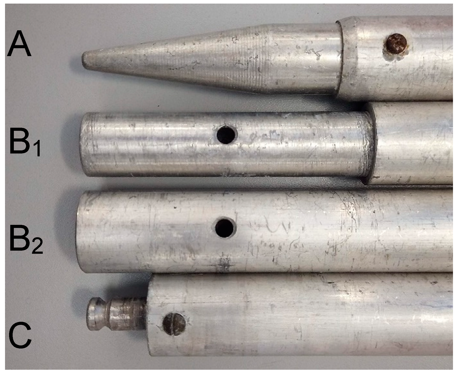
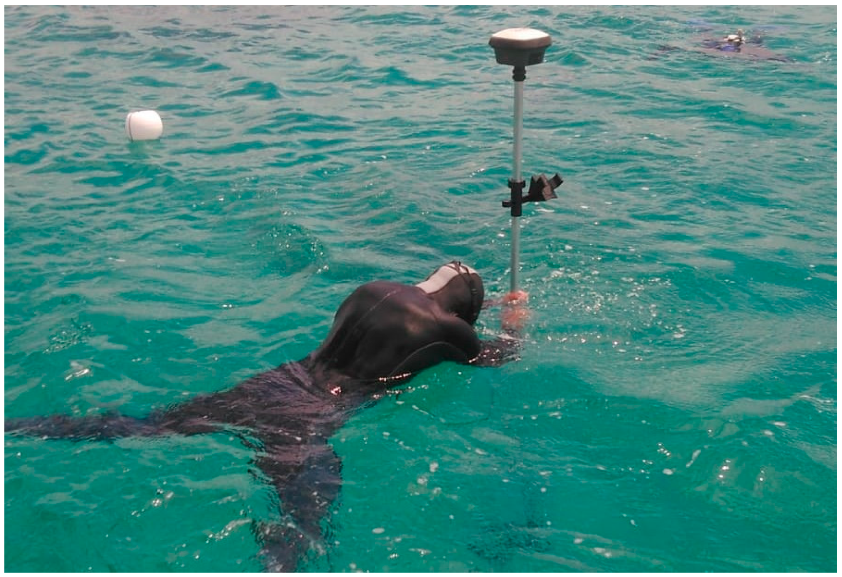
• The position of the markers is measured using an aluminum pole on top of which a GNSS receiver is installed in an N-RTK configuration (nominal accuracies of 2–3 cm in planimetry and 3–4 cm in altimetry when connected to the HxGN SmartNet network).
• A photogrammetric acquisition survey is carried out immediately after the markers have been placed.
• Steps 2 and 3 are repeated 24 h after the first measurement.

On the first day of the survey, marker coordinates were measured with GNSS (

Table 7. Marker coordinates measured via GNSS (tilt-compensated)—on the first day.

ID	Est [m]	Nord [m]	Elev [m]	σ Est [m]	σ Nord [m]	σ Elev [m]	Tilt [gon]	Tilt Max [gon]
F1	524,721.800	4,562,310.608	−2.675	0.009	0.011	0.024	5.026	11.390
F2	524,717.034	4,562,311.041	−2.488	0.009	0.010	0.022	5.628	13.333
F3	524,714.269	4,562,311.040	−2.336	0.008	0.010	0.022	7.597	7.638
F4	524,716.333	4,562,309.871	−2.415	0.009	0.010	0.023	0.100	6.440
F5	524,719.113	4,562,311.693	−2.564	0.008	0.010	0.022	2.544	6.538
F6	524,719.579	4,562,310.032	−2.539	0.010	0.012	0.029	2.898	2.898
F7	524,722.456	4,562,312.153	−2.755	0.008	0.010	0.022	4.190	4.190
F8	524,720.621	4,562,308.778	−2.507	0.009	0.010	0.023	4.186	5.750
F9	524,724.349	4,562,310.070	−2.811	0.008	0.010	0.022	3.760	6.684

) and TS (

Table 8. Marker coordinates measured via TS—on the first day.

ID	Est [m]	Nord [m]	Elev [m]
TS1	524,721.693	4,562,310.969	−2.770
TS2	524,717.044	4,562,311.249	−2.560
TS3	524,714.273	4,562,311.298	−2.398
TS4	524,716.951	4,562,310.427	−2.552
TS5	524,719.365	4,562,311.854	−2.626
TS6	524,719.789	4,562,310.096	−2.597
TS7	524,722.684	4,562,312.412	−2.812
TS8	524,720.835	4,562,308.815	−2.569
TS9	524,724.871	4,562,310.167	−2.871

).

The coordinates were inserted in Agisoft Metashape (version 1.8.5) to correspond to the markers to check their position. The GSD of the photogrammetric survey was 0.5 mm/pix. The RMSE resulting from the processing is 0.020 m for the coordinates acquired with the GNSS (tilt-compensated) and 0.299 m for the coordinates acquired with the TS. The absolute difference of the coordinates is reported in the following

Table 9. The discrepancy between marker coordinates was measured via GNSS and TS.

ID	Δ Est [m]	Δ Nord [m]	Δ Elev [m]
F1-TS1	0.107	−0.361	0.095
F2-TS2	−0.010	−0.208	0.072
F3-TS3	−0.004	−0.258	0.062
F4-TS4	−0.618	−0.556	0.137
F5-TS5	−0.252	−0.162	0.062
F6-TS6	−0.210	−0.064	0.058
F7-TS7	−0.228	−0.259	0.057
F8-TS8	−0.215	−0.037	0.062
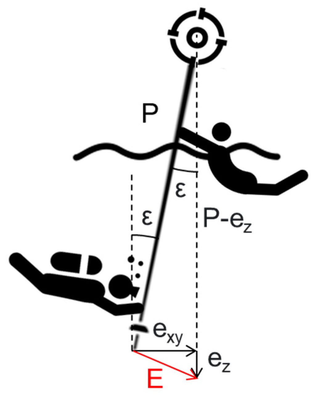
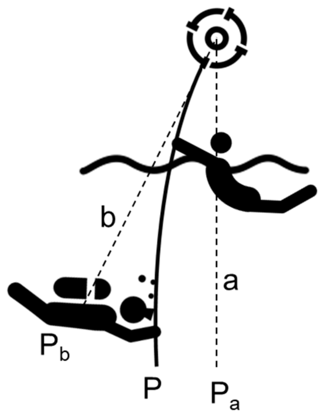
F9-TS9	−0.522	−0.097	0.060

. This behavior is expected as the side shot TS measurements suffer the plano-altimetric error previously described (Formula (1) and Table 3).

Another analysis concerns the stability of the conical markers, i.e., change of position on the seabed related to strong currents or other factors, such as flora and fauna disturbance or external human interactions (vessels or bathers unrelated to the survey operations). Therefore, the markers were re-measured with the GNSS N-RTK approach the following day, leaving them on the seabed overnight (

Table 10. Marker coordinates measured via GNSS (tilt-compensated)—second day.

ID	Est [m]	Nord [m]	Elev [m]	σ Est [m]	σ Nord [m]	σ Elev [m]	Tilt [gon]	Tilt Max [gon]
S1	524,721.804	4,562,310.635	−2.689	0.013	0.015	0.033	2.512	4.571
S2	524,717.082	4,562,311.091	−2.486	0.013	0.014	0.032	2.944	3.842
S3	524,714.305	4,562,311.094	−2.346	0.014	0.017	0.038	7.817	7.817
S4	524,716.349	4,562,309.891	−2.411	0.013	0.014	0.034	3.116	3.394
S5	524,719.129	4,562,311.703	−2.596	0.014	0.015	0.034	5.043	5.400
S6	524,719.620	4,562,310.105	−2.569	0.013	0.014	0.035	1.795	4.365
S7	524,722.385	4,562,312.189	−2.749	0.010	0.011	0.020	2.536	3.868
S8	524,720.625	4,562,308.745	−2.514	0.012	0.014	0.031	0.952	2.174
S9	524,724.322	4,562,310.054	−2.800	0.012	0.014	0.030	4.871	5.357

).

Table 8 shows the coordinate differences of all nine measured GCPs.

Table 11. Discrepancy difference between marker coordinates measured via GNSS—first day and second day.

ID	Δ Est [m]	Δ Nord [m]	Δ Elev [m]
F1-S1	−0.003	−0.028	0.014
F2-S2	−0.049	−0.050	−0.002
F3-S3	−0.036	−0.054	0.010
F4-S4	−0.017	−0.019	−0.004
F5-S5	−0.016	−0.011	0.032
F6-S6	−0.041	−0.073	0.030
F7-S7	0.071	−0.035	−0.006
F8-S8	−0.005	0.034	0.007
F9-S9	0.027	0.016	−0.011

shows that the difference between marker coordinates measured on the first and second days is relatively low and difficult to analyze as it coexists with the planimetric error of 2–3 cm and the altimetric error of 3–4 cm of the N-RTK survey.

To compensate for the GNSS systematisms, a comparison between point distances has been performed, as reported in the following

Table 12. Comparison between point distances measured via GNSS—first day and second day.

Distance	[m]	Distance	[m]	Distance Difference	[m]
D F1-2	4.790	D S1-2	4.746	Δ F-S 1-2	0.043
D F2-3	2.768	D S2-3	2.733	Δ F-S 2-3	0.036
D F3-4	2.372	D S3-4	23.78	Δ F-S 3-4	0.005
D F4-5	3.327	D S4-5	3.348	Δ F-S 4-5	0.021
D F5-6	1.724	D S5-6	1.666	Δ F-S 5-6	0.058
D F6-7	3.581	D S6-7	3.545	Δ F-S 6-7	0.036
D F7-8	3.850	D S7-8	3.877	Δ F-S 7-8	0.027
D F8-9	3.958	D S8-9	3.926	Δ F-S 8-9	0.031

.

The coordinates were inserted in Agisoft Metashape (version 1.8.5) to correspond to the markers to check their position. The GSD of the photogrammetric survey was 0.5 mm/pix. The RMSE resulting from the processing is 0.024 m, which is acceptable for the survey’s needs.

4. Discussions

The scholarly community’s burgeoning interest in surveying and monitoring submerged assets, encompassing archaeological sites, shipwrecks, and coral reefs, reflects a multifaceted pursuit to unravel the underwater world’s heritage. However, the exploration and documentation of these submerged realms are fraught with challenges, particularly in precise positioning and georeferencing. These challenges, stemming from the intrinsic characteristics of the underwater environment, necessitate innovative solutions and methodologies to overcome them effectively.

One of the foremost challenges encountered in underwater positioning endeavors is the propagation of electromagnetic waves in aquatic environments. Global Navigation Satellite Systems (GNSSs), including GPS, utilize electromagnetic waves for positioning. However, these waves undergo attenuation and refraction when traversing water mediums, resulting in inaccuracies and distortions in positioning data. The complex interplay between water’s physical properties and electromagnetic wave propagation poses a formidable obstacle to achieving a precise underwater positioning [21].

Furthermore, concerning the use of acoustic positioning, the phenomenon of multipath interference poses a problem for underwater positioning systems. Multipath interference occurs when electromagnetic waves reflect off multiple surfaces before reaching the receiver, leading to signal distortion and positioning errors. In shallow waters or areas with reflective surfaces, such as metallic shipwrecks, the impact of multipath interference is particularly pronounced, complicating positioning efforts and compromising data accuracy [22].

The cost and complexity of underwater positioning and georeferencing systems constitute additional challenges in this domain. Many existing methodologies and technologies for underwater positioning entail significant financial investment and operational intricacies, limiting their accessibility to researchers and stakeholders. These systems’ high cost and complexity pose barriers to widespread adoption and utilization, constraining the advancement of underwater surveying and monitoring endeavors.

Despite these formidable challenges, a growing demand exists for precise and reliable positioning and georeferencing solutions in the underwater domain. This demand is fueled by many factors, including the imperative to document and preserve submerged cultural heritage sites, such as ancient shipwrecks and underwater archaeological sites, and the pressing need to study and safeguard marine ecosystems and habitats [23].

Historically, attempts to address the complexities of underwater positioning have relied on trilateration via acoustic positioning systems, leveraging costly inertial sensors or acoustic beacons, or integrating a combined GNSS approach involving periodic drone surfacing [24]. While these methods have demonstrated utility in certain contexts, they are beset by inherent limitations, including compromised accuracy and restricted applicability in challenging underwater environments [25].

In response to these challenges, this research seeks to elucidate the constraints of GNSS-based positioning and georeferencing in lower-depth underwater environments while exploring avenues for innovation and improvement. By harnessing existing methodologies and pioneering novel instrumentation, the aim is to facilitate precise topographic surveys of ground control points (GCPs) and control points (CPs) in very shallow waters [26].

Central to this endeavor is developing and validating innovative prototypes such as PALONE and CONETTO, which represent significant underwater positioning technology advancements compared to similar solutions available in state of the art [17]. As shown in the tests performed in this research, the accuracy results obtained, combined with tilt-compensated GNSS devices or tilt-compensated topographic poles, are compliant with the requirements of the centimeter-grade accuracy survey, providing comparable outputs with the terrestrial use.

5. Conclusions

This study underscores the necessity for meticulously surveying and monitoring submerged assets, accentuating the imperative for using precise and dependable positioning and georeferencing methodologies. Recognizing the constraints inherent in conventional GNSS-based techniques, exploring alternative modalities, notably acoustic positioning and pressure sensing, has emerged as a pivotal focus. Such diversification of methodologies offers promising avenues to surmount the inherent challenges of subaquatic environments and foster heightened accuracy and reliability in underwater positioning.

Despite the impressive difficulties the marine environment presents, the potential for innovation and refinement in this sphere remains substantial. By amalgamating established methodologies with nascent technological paradigms, the scientific community is poised to address the intricacies of underwater positioning and georeferencing with greater efficacy. This necessitates a collaborative endeavor engaging researchers, engineers, and stakeholders to craft robust solutions capable of withstanding the rigors of marine environments.

Moreover, the ramifications of underwater positioning and georeferencing advancements extend beyond the confines of academic inquiry to encompass broader societal dividends. Enhanced accuracy and reliability in underwater navigation and cartography hold promise for facilitating the exploration and conservation of submerged heritage sites and marine ecosystems. Consequently, these attempts contribute to the broader imperatives of comprehending and safeguarding our subaqueous cultural and natural legacies for posterity.

Through concerted research and developmental undertakings grounded in a nuanced comprehension of the distinctive challenges and opportunities inherent to underwater data acquisition and processing, the scientific community stands poised to improve positioning and georeferencing toward unprecedented validation results.

6. Patents

The device described in this paper is in Section 2.1. (i.e., the conic underwater marker—CONETTO) is patent pending, meaning a provisional patent application has been filed to the Ministry of Enterprises and Made in Italy—Italian Patent and Trademark Office (UIBM)—ref. n. 102023000026709.