Coupling Downscaling and Calibrating Methods for Generating High-Quality Precipitation Data with Multisource Satellite Data in the Yellow River Basin

Abstract

Remote sensing precipitation data have the characteristics of wide coverage and revealing spatiotemporal information, but their spatial resolution is low. The accuracy of the data is obviously different in different study areas and hydrometeorological conditions. This study evaluated four precipitation products in the Yellow River basin from 2001 to 2019, constructed the optimal combined product, conducted downscaling with various machine algorithms, and performed corrections using meteorological station precipitation data to analyze the spatiotemporal trends of precipitation. The results showed that (1) GPM and MSWEP had the best four evaluation indicators, with R² values of 0.93 and 0.90, respectively, and the smallest FSE and RMSE, with a BIAS close to 0. A high-precision mixed precipitation dataset, GPM-MSWEP, was constructed. (2) Among the three methods, the downscaling results of DFNN showed higher accuracy. (3) The results, after correction with GWR, could more effectively enhance the accuracy of the data. (4) Precipitation in the Yellow River Basin showed a decreasing trend in January, September, and December, while it exhibited an increasing trend in other months and seasons, with 2002 and 2016 being points of abrupt change. This study provides a reference for the production of high-precision satellite precipitation products in the Yellow River basin.

1. Introduction

In recent years, a variety of satellite precipitation products have been generated successively, such as the Climate Hazards Group InfraRed Precipitation with Station data (CHIRPS), Global Precipitation Climatology Project (GPCP), Tropical Rainfall Measuring Mission (TRMM), Global Satellite Mapping of Precipitation (GSMaP), Climate Prediction Center Morphing technique (CMORPH), etc. [1,2,3,4]. Satellite precipitation products can provide continuous spatial and temporal distribution information of precipitation, which can compensate well for the shortage of meteorological station data. Since most gridded precipitation products have global (or quasi-global) coverage, their performance is expected to vary among regions [5,6,7,8,9,10]; McCollum et al. [11] pointed out that precipitation products of remote sensing satellites are different in terms of different algorithms and data resolutions in the process of retrieving precipitation due to different sensors on satellites. As a result, the regional applicability of different satellite precipitation products is different. Tang et al. [12] compared the applicability of TRMM and Global Precipitation Measurement Mission (GPM) products in mainland China and found that GPM products were superior to those of the TRMM and had better performance in middle and high latitude regions. Moreover, the accuracy and spatial resolution of satellite precipitation data are generally low, which cannot meet the further needs of refined hydrological and meteorological research [13].

At present, high-resolution remotely sensed precipitation data are still under development, and acquiring data information to meet high accuracy requirements is still facing difficulties [14]. The use of downscaling methods to obtain high-precision precipitation data can effectively meet the needs of regional-scale studies [15,16]. At the current stage, the main downscaling methods are dynamical downscaling methods and statistical downscaling methods. Dynamical downscaling methods are difficult to apply in downscaling to higher spatial resolutions [17]. In statistical downscaling methods, the accuracy and performance of machine learning algorithms in dealing with complex nonlinear problems have been proven to be significantly superior to traditional statistical regression models [18,19,20,21]. Several researchers have used various typical machine learning algorithms for downscaling experiments on TRMM precipitation data, mainly Classification and Regression Trees (CART), k-nearest neighbors (k-NN), support vector machines, and Random Forest (RF), where RF performs the best among the above machine learning algorithms [22,23]. In addition, the Boosting algorithm is considered to be one of the best performing methods in statistical learning [24]. The Gradient Boosting Decision Tree (GBDT) as a typical boosting algorithm can control the degree of fitting more carefully than RF to improve the simulation effect [25]. Compared to machine learning, deep learning has significant advantages in terms of the training cost and efficiency [26,27]. The Deep Feedforward Neural Network (DFNN) as a deep learning model has a good adaptive learning ability for complex multiple-input multiple-output nonlinear problems. However, at present, RF is the main machine learning algorithm commonly used in precipitation downscaling, while other algorithms such as GBDT and DFNN have less research on downscaling, and the performance of these methods needs further research.

The accuracy of satellite precipitation products is affected by several factors, such as the precipitation type, topographic conditions, and spatial and temporal scales. Most satellite precipitation products have the problem of overestimating light rainfall and underestimating heavy rainfall [28]. In recent years, some methods of multisource data fusion have been developed to improve the spatial and temporal resolution and accuracy of precipitation data. Cheema et al. [29] used Geographical Difference Analysis (GDA) and regression analysis for the local calibration of TRMM precipitation in the Indus basin and found that the GDA method was better after calibration. Duan et al. [30] used the Geographical Ratio Analysis (GRA) method to correct the precipitation data of Ethiopian and Iranian coastal areas, and concluded that both methods were effective in reducing the BIAS between satellite products and meteorological station data. However, due to the uneven distribution and low density of meteorological stations in some regions, it is difficult to apply them to the study of the refined spatial and temporal variability characteristics of precipitation. In recent years, Yu et al. [31] carried out a study on precipitation in the Hengduan Mountains region to analyze the relationship between the spatial and temporal distribution characteristics, latitude, and elevation. Khan et al. [32] examined the trend characteristics and mutation points of the 95% and 99% extreme precipitation series in the Indian continent for the years 1901–2015 by using Mann–Kendall’s method and the Bernaola Galvan (B-G) segmentation algorithm, and found that the region’s extreme precipitation has a significant temporal trend and shows an opposite trend before and after the mutation time point. Therefore, after downscaling, it is essential to fully utilize meteorological station data for data verification, and to conduct spatiotemporal analysis on the results of the downscaling verification.

In this study, based on various satellite precipitation data, we compare their applicability in the Yellow River basin, establish statistical downscaling models between precipitation and vegetation elements and geographic factors using various machine learning methods, and calibrate the downscaled results with meteorological station data. Finally, the spatial variation and temporal trends of precipitation in the Yellow River basin are analyzed. The main objectives of this study are as follows: (1) Perform a suitability analysis of precipitation products to construct a high-precision mixed dataset GPM-MSWEP. (2) Downscale GPM-MSWEP data with better applicability at 0.1° resolution to obtain 1 km high-resolution precipitation data using multiple machine learning models. (3) Perform a GDA based on the difference between downscaled data and meteorological station data. Using the difference data as independent variables and the corresponding downscaled results as dependent variables, a Geographically Weighted Regression (GWR) model is constructed to individually calibrate the downscaled data. (4) The stage characteristics of annual precipitation, and spatial trends of monthly and seasonal precipitation in the Yellow River basin are analyzed. The results of the study can provide a scientific basis for drought and flood control and water resources management optimization in the Yellow River basin.

2. Materials and Methods

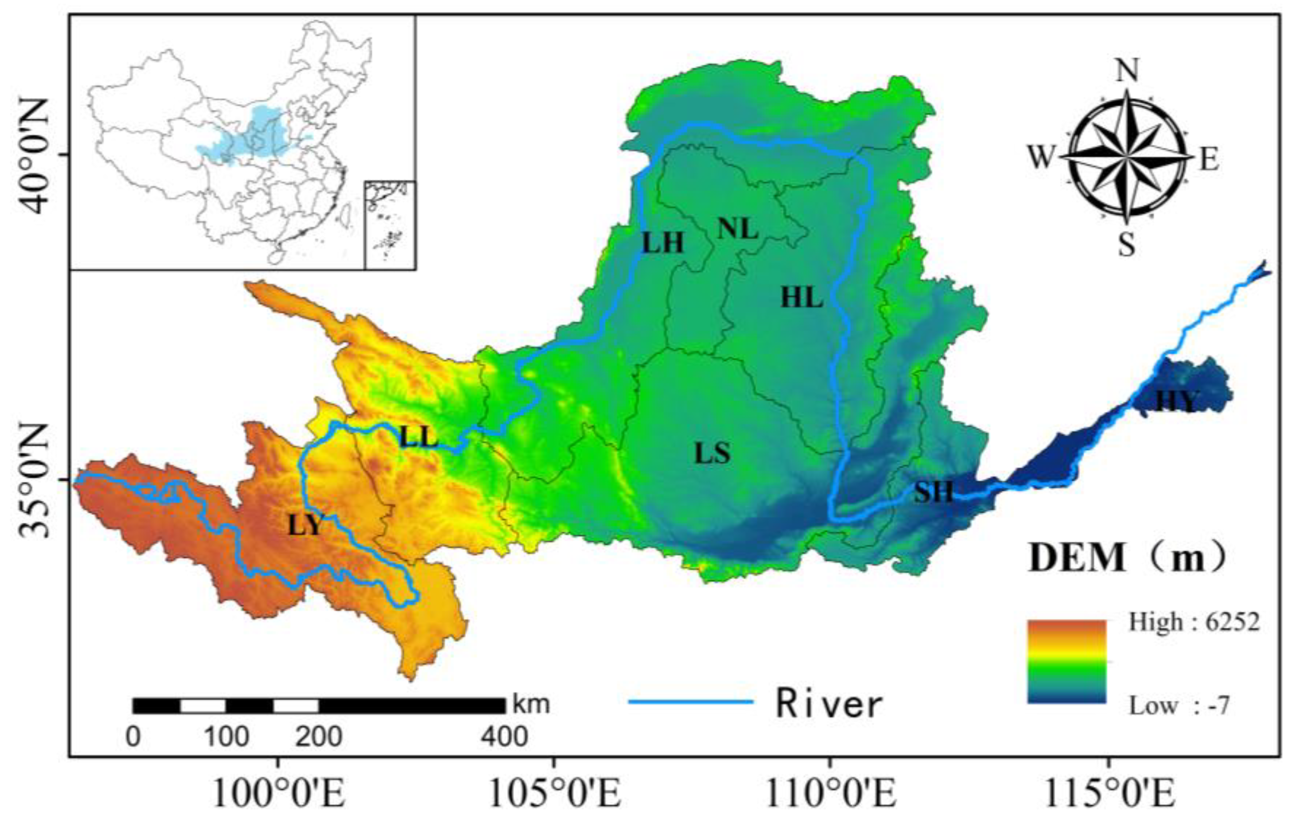
2.1. Study Area

The Yellow River basin (96°–119°E, 32°–42°N) runs through the north-central part of China, with a watershed area of approximately 752,443 km² and a total length of approximately 5464 km. The basin encompasses high-altitude plateaus, deeply incised loess plateaus, vast plains, as well as mountainous and hilly areas, ultimately forming a delta at the river mouth. Due to the wide range of regional climates and the influence of atmospheric circulation and monsoons, there is significant climate variability within the basin. Precipitation mainly occurs from June to October, with uneven distribution throughout the year, and an average annual precipitation of approximately 466 mm. As shown in Figure 1, there are 8 secondary water resource divisions in the Yellow River basin, including LY, LL, LH, NL, HL, LS, SH, and HY.

2.2. Data

2.2.1. Remote Sensing Precipitation Data

In this paper, the data were preprocessed using cropping and projection conversion, unit conversion, and other preprocessing operations to obtain monthly, quarterly, and annual precipitation data. The CHIRPS V2.0 dataset from January 2001 to December 2019 was chosen as the data for the study. The CHIRPS precipitation product (Climate Hazards Group InfraRed Precipitation with Station data) is a joint development of the University of California Climate Hazards Group and the United States Geological Survey (USGS). It is a precipitation dataset with global coverage, and the data were downloaded from ftp://ftp.chg.ucsb.edu/pub/org/chg/products/CHIRPS-2.0 (accessed on 11 January 2023) with a temporal resolution of months and a spatial resolution of 0.25°.

Multisource Weighted-Ensemble Precipitation (MSWEP) is a global precipitation product generated by Beck’s team using multivariate precipitation observations. The MSWEP dataset from January 2001 to December 2019, version V2.8 research data, was downloaded from the GloH2O data platform http://www.gloh2o.org/(accessed on 13 January 2023). The dataset files were stored in “netcdf” format with time resolution of 3 h and a spatial resolution of 0.1°.

The Tropical Precipitation Observation Program (TRMM) for precipitation data was launched in November 1997 as a collaboration between NASA and the Japan Aerospace Exploration Agency (JAXA). TRMM offers a range of algorithmically processed products covering the region from 50°N to 50°S. One dataset, 3B43V7, has a spatial resolution of 0.25° and a temporal resolution of months as research data. Monthly TRMM 3B43 V7 precipitation data from January 2001 to December 2019 were downloaded from http://pmm.nasa.gov/data-acces/downloads/trmm (accessed on 13 January 2023).

GPM is the successor mission to TRMM, launched in February 2014, and aims to provide a new generation of global satellite precipitation observations. IMERG is a tertiary product of GPM, which fuses all satellite microwave sensor precipitation estimates with a spatial resolution of 0.1° based on infrared satellite observations, ground-based monthly rainfall information, and other precipitation estimates. GPM 3IMERG monthly precipitation data from January 2001 to December 2019 were downloaded from the website https://pmm.nasa.gov/data-access/downloads/gpm (accessed on 14 January 2023).

2.2.2. Meteorological Station Precipitation Data

Meteorological station precipitation data were obtained from the monthly dataset of Chinese terrestrial climate data provided by the China Meteorological Data Network (http://data.cma.cn/ (accessed on 11 January 2023)). The dataset contains climate data from 613 benchmark ground-based meteorological observation stations and automatic stations in China since 1951. The statistics have been manually checked to ensure the consistency of extreme values with time. We obtained monthly precipitation data of 81 stations from 2001 to 2019, and utilized the spatial interpolation software (ANUSPLIN 4.4) for climate data, to obtain a monthly raster -based precipitation dataset with 1 km spatial resolution.

2.2.3. DEM and NDVI Data

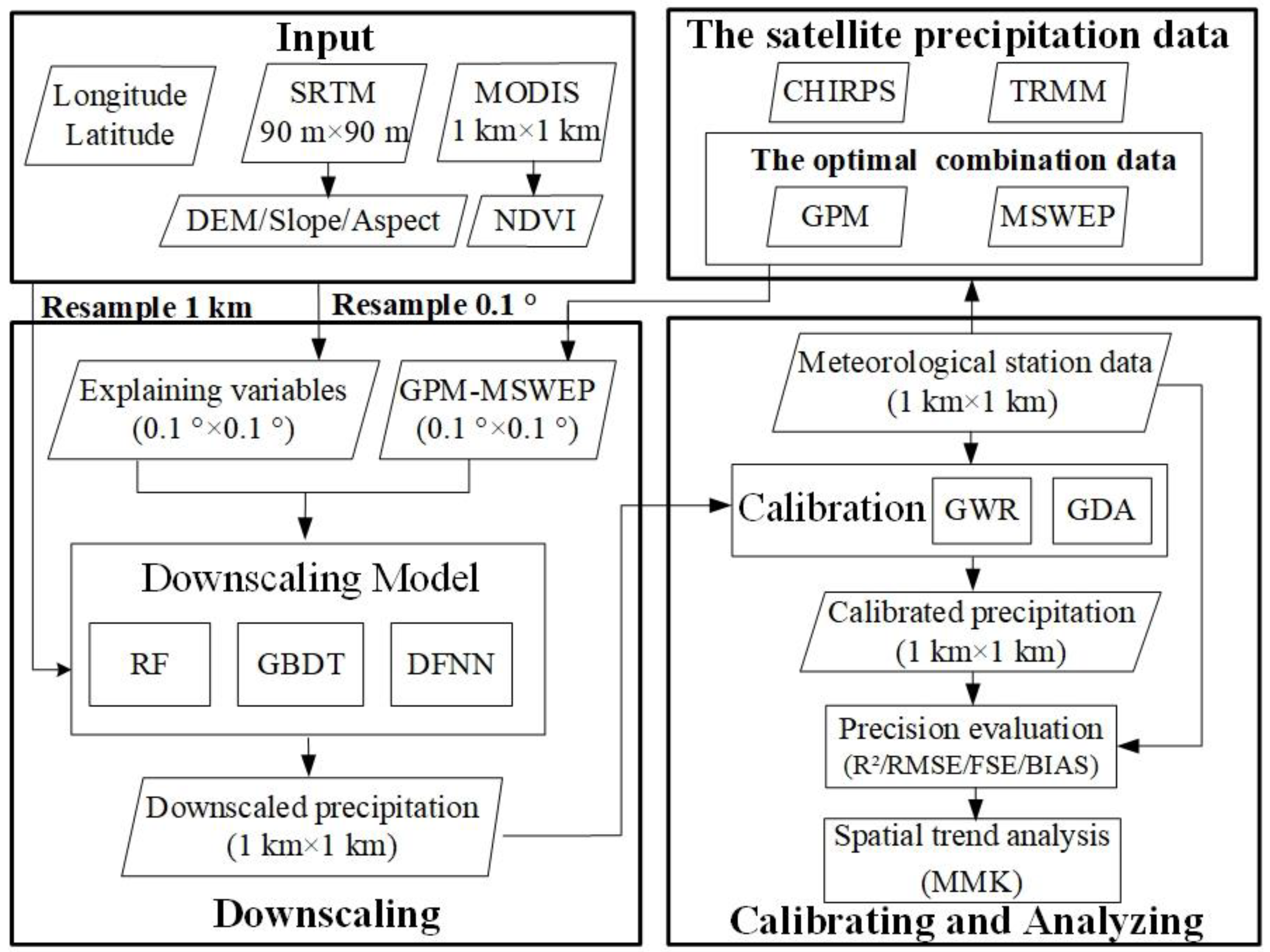
Digital Elevation Model (DEM) data from the Shuttle Radar Topography Mission (SRTM) were selected for this study, measured by NASA and the Department of Defense National Mapping Agency (NIMA). SRTM data at 90 m resolution were used in this study, and these data were downloaded from http://www.gscloud.cn/ (accessed on 16 January 2023). The data were preprocessed using ArcGIS 10.2 software for projection, clipping, and resampling to obtain elevation data at 0.1° and 1 km resolution for the study area, from which other topographic indices, including slope, slope direction, and latitude and longitude, were extracted.

Vegetation growth is one of the key explanatory variables for precipitation. The Normalized Difference Vegetation Index (NDVI), as an indicator of vegetation spatial distribution, has been proven by numerous studies to have a good correlation with regional precipitation. The NDVI data selected for this study were MOD13A3 products with a spatial resolution of 1 km, resampling of 0.1°, and a temporal resolution of months for the period from January 2001 to December 2019; they were downloaded from https://ladsweb.modaps.eosdis.nasa.gov/search/ (accessed on 16 January 2023).

2.3. Methodology

Figure 2 illustrates the flowchart of the proposed research procedures in this study, including comparative accuracy assessment analyses of multisource satellite precipitation data (CHIRPS, TRMM, MSWEP, and GPM); downscaling studies based on multiple machine-learning methods (RF, GBDT, and DFNN); and calibration of the downscaled results and characterization of the spatial trends in precipitation.

2.3.1. Downscaling Method

In this section, three different types of machine learning algorithms were used, namely, Random Forest based on Bagging algorithm, gradient boosting based on Boosting algorithm and Deep Feedforward Neural Network algorithm. The performance of the three algorithm models in the study area was analyzed and is compared in the later section.

RF, a representative of Bagging algorithm, was first proposed by Breiman [33] and has been widely used in various fields. The algorithm consists of several Classification and Regression Trees (CARTs), which effectively reduces the correlation between each tree and improves the accuracy of the regression model while reducing the variance due to the use of random perturbation method to select the features, and has the advantages of fast training speed and less overfitting [34]. Random forests are initially constructed by extracting approximately two-thirds of the dataset for training the model, and numerous decision trees are constructed to create a forest on which N_try node indicators are randomly selected. The final model predictions are made by taking the average of the prediction results of each regression tree. It can predict multiple factors and fit nonlinear relationships, so it performs well with downscaled meteorological data such as precipitation and temperature data [35,36].

$$f\left(m\right)=\frac{1}{T}{\sum }_{k=1}^{T}f\left(m,{\theta }_k\right)$$

(1)

where $m$ is the input variable, $T$ is the number of CART regression trees, ${\theta }_k$ represents the random variable of the kth tree independently and is identically distributed, $f\left(m,{\theta }_k\right)$ represents the prediction result of the kth tree, and $f\left(m\right)$ represents the final prediction result of the model.

The unsampled one-third of the sample is called out-of-bag (OOB) data and is used to generate a test set for estimating the model error [37].

$${MSE}_{oob}=\frac{1}{n}{\sum }_{i=1}^n{\left(y_i-f_{oob}\left(x_i\right)\right)}^2$$

(2)

where ${MSE}_{oob}$ is the model error, n is the number of OOB samples, and $f_{oob}\left(x_i\right)$ represents the model prediction value of the ith OOB sample.

GBDT model is an integrated learning algorithm proposed by Friedman et al. [38] that uses a decision tree as the underlying learner, which is a typical Boosting algorithm. GBDT follows the principle of no put-back sampling in the training process, and the base models are built using serial construction between them. The GBDT algorithm can be roughly divided into the following three steps: firstly, a simpler model is used as the initial classifier; secondly, the negative gradient of the loss function of each sample point under the current model is calculated, these negative gradients are used as the target variables to train a new weak classifier, the new classifier is added to the original model, and they are combined using weighted average or other methods; finally, when the GBDT model completes the pre-defined convergence conditions, it is combined with all the base learning models to form a strong learner. The process of the GBDT algorithm is described in detail below.

First, the initialized weak learner is created.

$$f_0\left(x\right)={argmin}_c{\sum }_{i=1}^{N}L(y_i,c)$$

(3)

where the loss function uses the mean-squared error function as follows:

$$L\left(y,f\left(x\right)\right)={\left(f\left(x\right)-y\right)}^2$$

(4)

where $f\left(x\right)$ is the predicted value, y is the true value, $L(y_i,c)$ is the loss function to calculate the difference between the target value and the simulated value, and c is the optimal parameter for minimizing the loss function. Then, for each sample i = 1, 2, ···, N, r_im negative gradient (residual) m = 1, 2, ···, M is calculated for m iterations.

$$r_{im}=-\left[\frac{\partial L(y_i,f(x_i\left)\right)}{\partial f\left(x_i\right)}\right]$$

(5)

The obtained negative gradients are used as true values and the data (x_i, r_im), i = 1, 2, ···, N are used as training data to fit a new regression tree f_m(x). In order to minimize the loss function of the new regression tree, the best-fit value corresponding to the leaf node region R_jm needs to be calculated.

$${\beta }_{jm}={argmin}_{\beta }\sum _{x_i\in R_{jm}}L(y_i,f_{m-1}\left(x_i\right)+\beta )$$

(6)

where R_jm, j = 1, 2, ···, J is the leaf node region and J is the number of leaf nodes in the regression tree.

Update Strong Learner.

$$f_m\left(x\right)=f_{m-1}\left(x\right)+{\sum }_{j=1}^J{\beta }_{jm}|x_i\in R_{jm}$$

(7)

Gradient Boosting Decision Tree.

$$f\left(x\right)=f_m\left(x\right)=f_0\left(x\right)+{\sum }_{m=1}^M{\sum }_{j=1}^J{\beta }_{jm}|x_i\in R_{jm}$$

(8)

DFNN, also called Feedforward Neural Network or multilayer perceptron and used in this paper, is a typical deep learning model. Layer 0 of this model is the input layer, the last layer is the output layer, and the other intermediate layers are called hidden layers, each of which consists of several neurons [39]. In Feedforward Neural Networks, the data flow is unidirectional, i.e., the neurons in each layer can only output data to the neurons in the next layer, without any influence or feed-back to the previous layer. The parameters to be debugged are the number of hidden layers, the number of neurons, and the number of iterations.

The neuron structure of each layer has the following mapping relationship:

$$y=f(x,{\theta }_0)$$

(9)

where x and y denote the input and output, respectively, and ${\theta }_0$ denotes the optimal parameter solution in the mapping relationship.

In this paper, Normalized Vegetation Index (NDVI), elevation (DEM), slope, aspect, longitude (LON), and latitude (LAT) were selected as the explanatory variables for constructing the model, and GPM-MSWEP precipitation data were used as the dependent variables to construct the downscaling model.

2.3.2. Data Calibration Method

GDA is a data calibration method proposed by Cheema and Bastiaansen [29], which is used to calibrate geographic information data to improve data accuracy by exploring the difference between actual data and geographic information data. The steps are as follows.

(1)

Calculate the difference between downscaled data and meteorological station data.

(2)

Interpolate the point difference data into a 1 km resolution raster data using ordinary kriging.

(3)

The 1 km resolution precipitation predicted by the model is added to the 1 km resolution difference data in (2) to obtain the 1 km resolution precipitation data calibrated using meteorological station data.

GWR is a local linear regression method proposed by Brunsdon [40]. In this paper, adaptive bisquared was chosen as the kernel function and the small-sample BIAS-calibrated AICC was used as the criterion to establish a geographically weighted regression model by considering the spatial weights between spatially adjacent points while estimating the parameters of the dependent and explanatory variables at each location. The basic formula is as follows:

$$y_i={\beta }_0\left(v_i,u_i\right)+{\sum }_{t=1}^n{\beta }_t\left(v_i,u_i\right)x_{it}+\epsilon \left(v_i,u_i\right)$$

(10)

where $y_i$ is the precipitation of the dependent variable at the ith sample point; $x_{it}$ is the observed value of the ith sample point of the tth independent variable; $\left(v_i,u_i\right)$ denotes the latitude and longitude coordinates of the ith sample point; ${\beta }_t\left(v_i,u_i\right)x_{it}$ is the regression parameter of the constant term at the ith sample point; $\epsilon \left(v_i,u_i\right)$ is the linear regression parameter of the tth influence factor on the ith sample point; $\epsilon \left(v_i,u_i\right)$ is the residual value calculated by the model at the ith sample point; and n is the number of sample points.

2.3.3. Precision Evaluation

In this paper, meteorological station data were used as the criteria to evaluate the accuracy of satellite precipitation and downscaled results, and correlation determination (R²), root-mean-square error (RMSE), fractional standard error (FSE), and relative mean bias (BIAS) were selected as the evaluation indexes. The coefficient of determination (R²) represents the correlation between the variables, ranging from 0 to 1, and the closer the value is to 1, the stronger the correlation between the two sets of data; the root-mean-square error (RMSE) can be used to reflect the deviation between the satellite precipitation data and the meteorological station data, and the closer the value is to 0, the smaller the deviation of the satellite precipitation data is and the higher the accuracy is; the fractional standard error (FSE) is a dimensionless index, with smaller values indicating a smaller error in satellite precipitation data; the relative deviation BIAS was used to evaluate the deviation of satellite precipitation data compared with the measured precipitation data, and a value greater than 0 indicates an overestimation of satellite precipitation, while a value less than 0 indicates an underestimation of satellite precipitation. The calculation formula of each index is as follows:

$$R^2={\left(\frac{\sum (S-\overline{S})(G-\overline{G})}{\sqrt{\sum {(S-\overline{S})}^2\sum {(G-\overline{G})}^2}}\right)}^2$$

(11)

$$RMSE=\sqrt{{\frac{1}{n}{\sum }_{i=1}^n(S_i-G_i)}^2}$$

(12)

$$FSE=\sqrt{\frac{\frac{1}{n}\sum _{i=1}^n{(S_i-G_i)}^2}{\frac{1}{n}\sum _{i=1}^n{G}_i}}$$

(13)

$$BIAS=\frac{\frac{1}{n}{\sum }_{i=1}^n(S_i-G_i)}{{\sum }_{i=1}^n{G}_i}\times 100\mathrm{\%}$$

(14)

where n is the length of data series; S is satellite precipitation data (mm); G is measured precipitation data (mm); $\overline{S}$ is the average value of satellite precipitation data (mm); and $\overline{G}$ is the average value of measured precipitation data (mm).

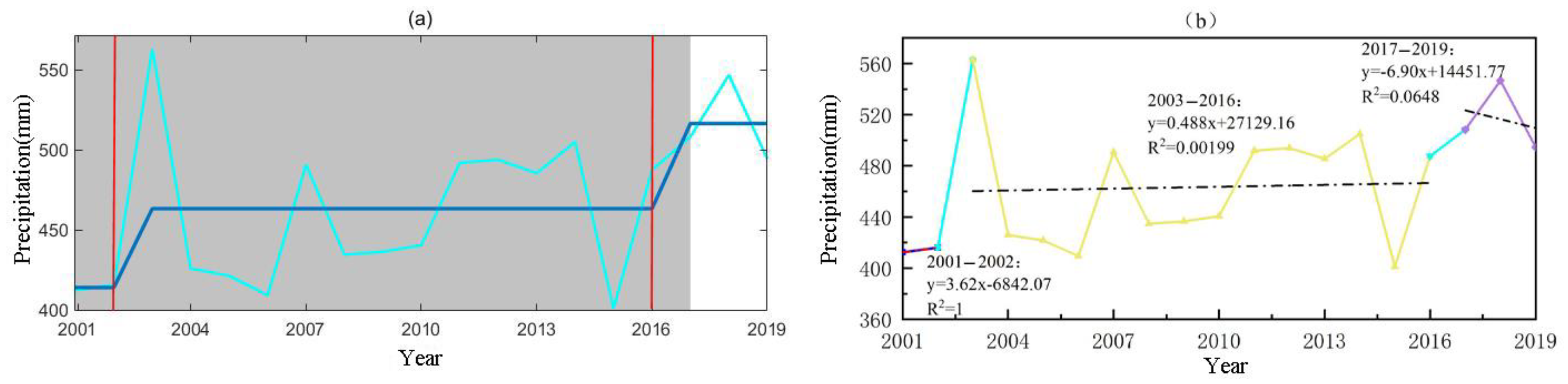
2.3.4. Analysis of Stages and Trends

The BG segmentation algorithm is a suitable method for detecting mutations in nonlinear time series proposed by Bernaola-Galvan et al. [41]. In this paper, the B-G segmentation algorithm was applied to detect mutations in the precipitation time series of the Yellow River basin for the years 2001–2019 and to divide them into different phases in order to explore the characteristics of the changes in precipitation at different phases. The specific steps of the algorithm are as follows:

(1) The length of the time series is N; two segments of the same interval before and after point $i$ are averaged and denoted as $U_L$ and $U_R,$ respectively, ($i=2,3,\dots .,N-1$).

(2) Calculate the statistic to reflect the difference between the two $U_L$ and $U_R$:

$$T\left(i\right)=\left(U_L-U_R\right)/S_D$$

(15)

$$S_D={\left[\left(S_L^2+S_R^2\right)/\left(N_L+N_R-2\right)\right]}^{1/2}{\left(1/N_L+1/N_R\right)}^{1/2}$$

(16)

where $N_L$ and $N_R$ are the number of samples in the two segments before and after the split point; $S_L$ and $S_R$ are the standard deviations of the segments divided into the two segments before and after the split point; and $S_D$ is the joint variance.

(3) Determine the maximum value in the statistic $T\left(i\right)$ and denote it as T2 and calculate the statistical significance of $T_m$ $P\left(T_m\right)$:

$$P\left(T_m\right)=\mathrm{P}\mathrm{r}\mathrm{o}\mathrm{b}\left(T\le T_m\right)$$

(17)

According to Monte Carlo simulation it can be obtained using

$$P\left(T_m\right)\approx {\left(1-I_{\mu /\left(\mu +T_m^2\right)}(\theta v,\theta )\right)}^{\alpha }$$

(18)

where $N$ is the length of the time series $x\left(t\right)$; $\mu =N-2;\theta =0.4$; $\alpha =4.19\mathrm{l}\mathrm{n}N-11.54$; $I_x(a,b)$ is the incomplete $\beta$ function; and the significance level takes a value of 0.95.

(4) If the $T_m\left(i\right)$ obtained in the previous step passes the significance test, the time series is divided into two sub-sequences according to the segmentation points, and other segmentation points can be detected by repeating the above steps.

The traditional Mann–Kendall trend test (MK) is a nonparametric statistical test that detects the trend characteristics of a time series [42]. It is based on the assumption that time series are random and independent. This affects the precision of the results due to the existence of autocorrelation in the time series. Modified Mann–Kendall trend test (MMK) has the ability to eliminate the autocorrelation in the series, significantly improving the testing power of the MK method [43]. It is now widely used in areas such as water and drought meteorology. When the MMK statistic S > 0, S = 0, S < 0, the equation is as follows:

$$Z^{*}=\left\{\begin{array}{c}\frac{S-1}{\sqrt{va{r}^{*}\left(S\right)}}\hspace{1em}\hspace{1em}S>0\\ \hspace{1em}\hspace{1em}0\hspace{1em}\hspace{1em}\hspace{1em}S=0 \\ \frac{S+1}{\sqrt{va{r}^{*}\left(S\right)}}\hspace{1em}\hspace{1em}S<0\end{array}\right.$$

(19)

The trend statistic $Z_s$ indicates that the time series is trending upward and $Z_s<0$ indicates that the time series is trending downward. When ${|Z}_s|$ is greater than or equal to 1.96 and 2.58, it indicates that the significance test with 95% and 99% confidence level is passed, respectively.

3. Results

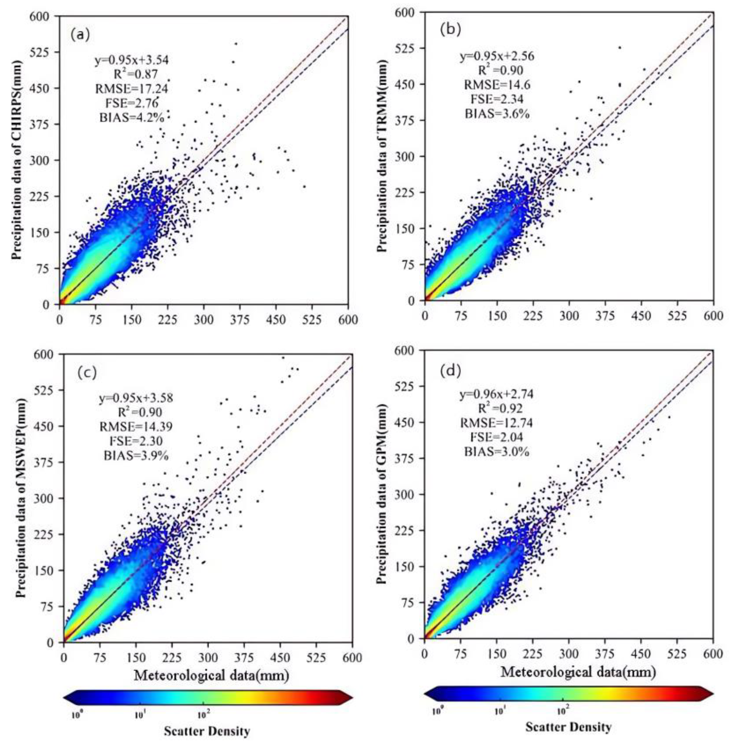
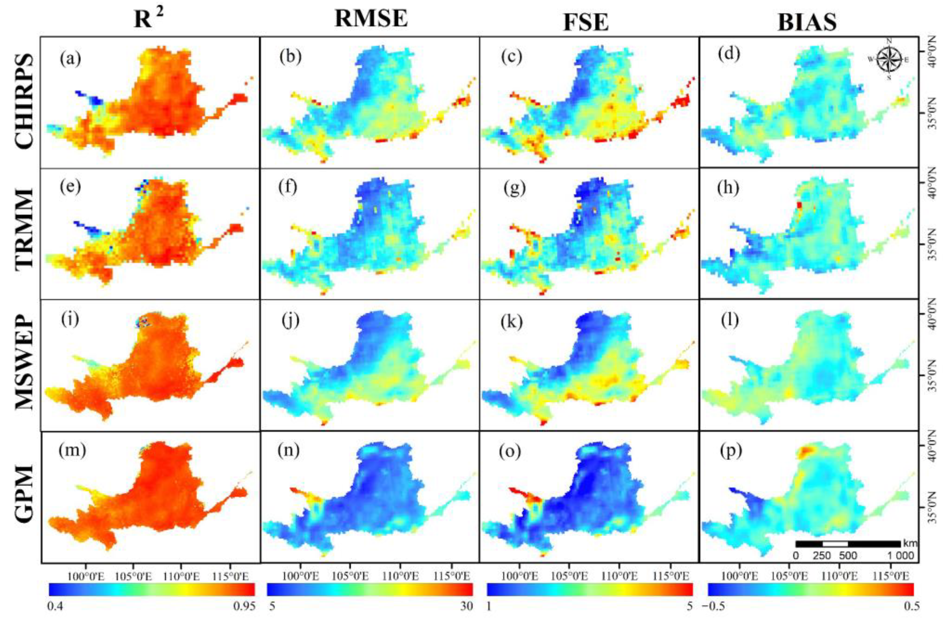
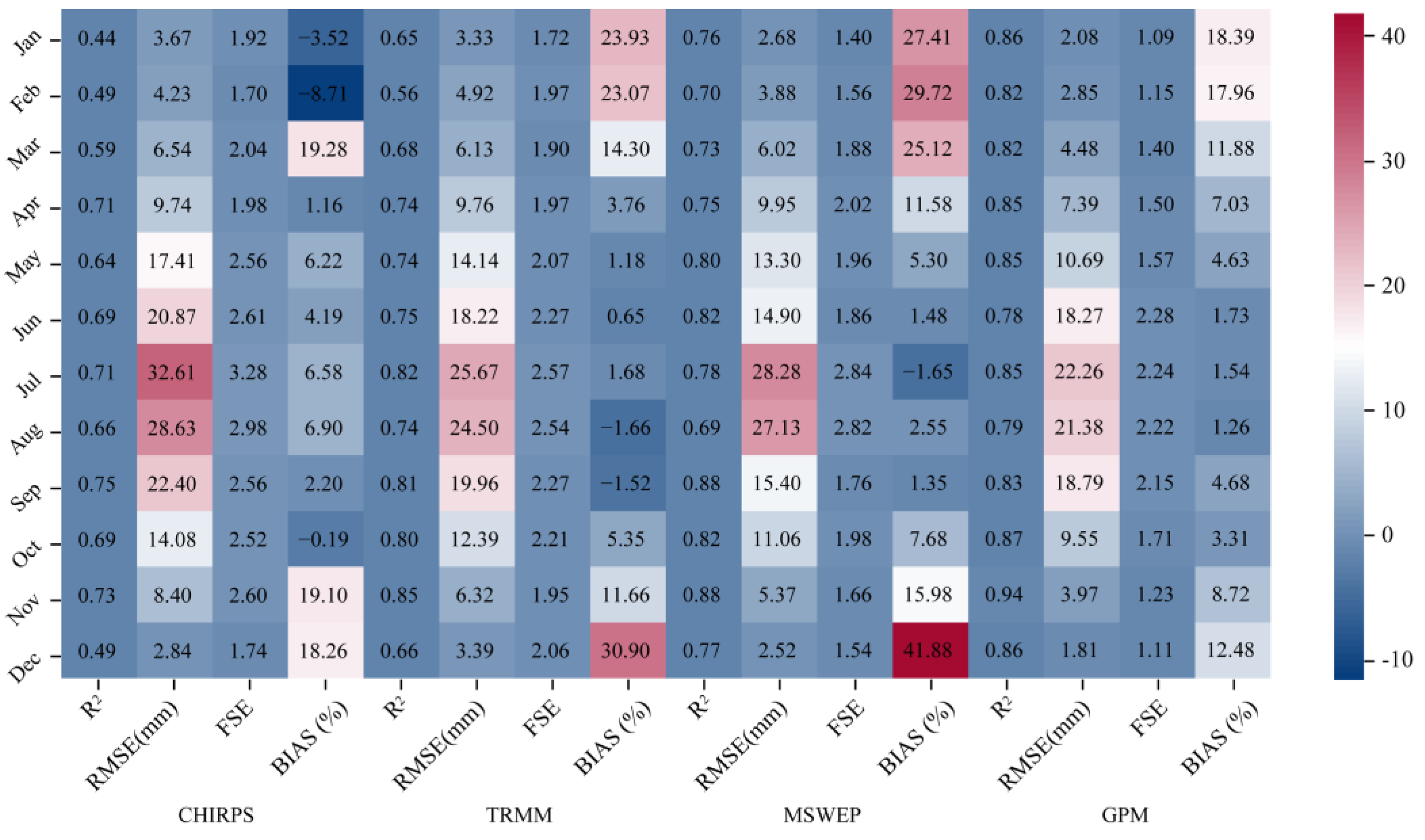
3.1. Optimal Combination of Remotely Sensed Precipitation Dataset

Figure 3 displays the precision evaluation outcomes of the CHIRPS, TRMM, MSWEP, and GPM precipitation data alongside the meteorological station data. A conspicuous correlation existed among these datasets, reflected by R² values surpassing 0.87. In specific terms, the GPM data boasted the loftiest R² value at 0.92. The TRMM and MSWEP data exhibited R² values of 0.90, whereas the CHIRPS data showcased the weakest correlation, with an R² of 0.87. From the perspective of the root-mean-square error (RMSE), the CHIRPS data registered the highest RMSE of 17.24 mm. Comparatively, the TRMM and MSWEP data demonstrated RMSEs of 14.6 mm and 14.39 mm, respectively. The GPM data recorded the smallest RMSE at merely 12.74 mm, implying minimal precipitation estimation error. Regarding the fractional standard error (FSE), the CHIRPS data had the largest FSE of 2.76 mm, indicating relatively commendable performance when juxtaposed with the TRMM, MSWEP, and GPM data (2.34, 2.30, and 2.04, respectively). With respect to relative BIAS, these four datasets spanned from 3.0% to 4.2%, denoting a general tendency to overestimate monthly precipitation in the Yellow River basin. Among these, the CHIRPS data performed most unfavorably, showcasing the greatest overvaluation at approximately 4.2%. Conversely, the GPM data exhibited the smallest deviation, with merely 3.0%, showcasing commendable alignment. Overall, on the monthly scale, the precision of these four satellite precipitation datasets exhibited both strengths and limitations. The GPM–meteorological station data correlation was the strongest, with minimal RMSE and FSE values and negligible BIAS, suggesting a relatively modest degree of precipitation overestimation. Conversely, the CHIRPS data performance was comparatively unsatisfactory concerning the coefficient of determination, RMSE, FSE, and relative deviation.

Figure 4 shows the spatial distribution of four precision evaluation indexes in the Yellow River basin. The accuracy evaluation indexes of these satellite precipitation products showed similar characteristics in spatial distribution. Among them, the distribution trend of R² of the four determinants was similar, and the R² value was obviously higher in the eastern and southern regions with more precipitation. In the whole basin, the R² distribution of the GPM data was better, and the range of high value areas was wider. The RMSE and FSE of the CHIRPS, TRMM, and MSWEP data all showed similar spatial variation. The RMSE and FSE of GPM data were evenly distributed. In the spatial distribution of the relative BIAS of the four satellite precipitation products, the BIAS value of the GPM data in the whole Yellow River basin was generally low. Approximately 75.84% of the basin area had a relative BIAS value in the range of −10% to 10%. The BIAS value of the TRMM data was generally high, and approximately 48.70% of the basin area had a relative BIAS value in the range of −10% to 10%. In general, the overestimation of precipitation using four kinds of satellite precipitation products mainly occurred in the western part of the upper reaches, the southeastern part of the middle reaches, and some parts of the lower reaches. The relative BIAS value of the MSWEP data was in the range of −10% to −10% in approximately 66.39% of the basin area, and the overestimation phenomenon mainly occurred in the middle and lower reaches of the basin. The TRMM data underestimated the precipitation in the upper reaches of the basin, and overestimated the precipitation in the middle and lower reaches of the basin.

Figure 5 shows the results of the coefficient of determination (R²), root-mean-square error (RMSE), fractional standard error (FSE), and relative BIAS assessment for each month of the CHIRPS, TRMM, MSWEP, and GPM precipitation data from 2001 to 2019. According to this, it can be observed that GPM data showed significant advantages in all four evaluation indicators in March, April, July, August, November, and December. The relative deviation of CHIRPS data in January and February was the smallest among the four precipitation datasets, at −3.52% and −8.71%, respectively. The relative deviation of TRMM data in May and June was the smallest, at 1.18% and 0.65%, respectively. In contrast, the MSWEP data showed better applicability, with a performance of R² = 0.82, RMSE = 14.90 mm, and FSE = 1.86 in June, and R² = 0.88, RMSE = 15.40 mm, FSE = 1.76, and BIAS = 1.35% September. In order to obtain the most accurate precipitation dataset before downscaling, the data in June and September of MSWEP were used to replace those two months of data in the GPM dataset in order to generate a new dataset named GPM-MSWEP.

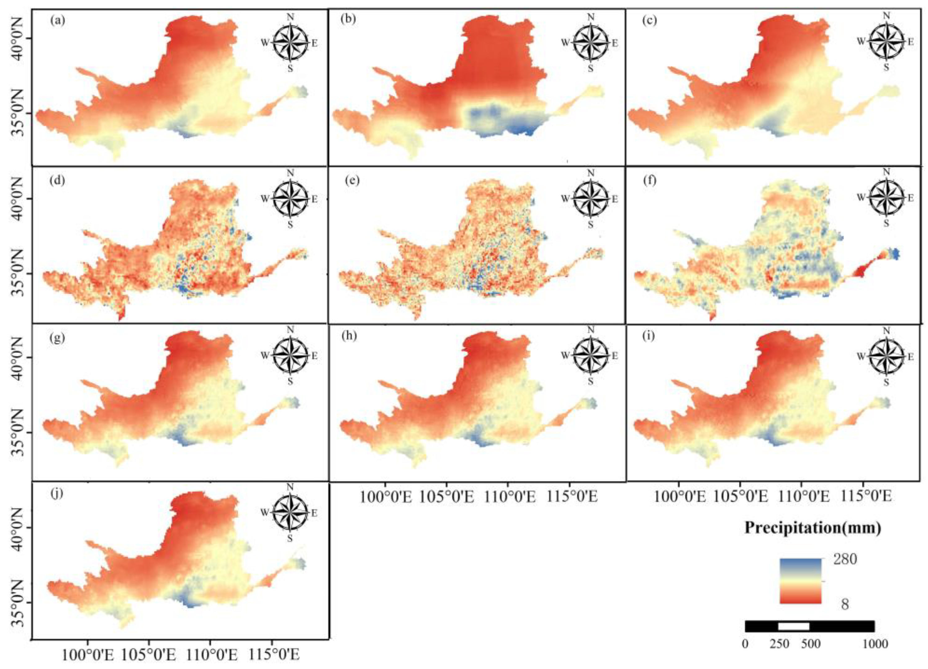
3.2. Downscaled Results

Figure 6 show the downscaled results for July 2012 using the Random Forest, Gradient Enhancement, and Deep Feedforward Neural Network algorithm, respectively. It can be clearly observed from these images that the images after downscaling are significantly better than the original satellite images in terms of spatial resolution and fineness. The precipitation data predicted using the three machine learning models were basically consistent with the original satellite image data in the spatial distribution of precipitation, with good spatial detail, and better presenting the regional local precipitation differences. Compared with Figure 6j, it can be clearly seen that the DFNN algorithm model and the RF algorithm model based on the Bagging method had a better scaling effect in terms of the spatial distribution than the GBDT algorithm model based on the Boosting method. The downscaled results of the DFNN algorithm model and the RF algorithm model can reflect the regional precipitation change more accurately.

It can be observed from Figure 6d–f that the residual distribution of the three machine learning models presents an obvious regularity. In the downscaled results, the underestimation region (that is, the region with high residual value) was mainly concentrated in the central and southern regions. Among the downscaling residuals of the three models, the residuals of the RF model (Figure 6d) and the GBDT model (Figure 6e) are clustered and spatially consistent, while the spatial distribution of the residuals of the DFNN model (Figure 6f) is discrete and lacks an obvious regularity. In addition, through the range of residuals, it can be observed that the downscaling residuals of the DFNN model were relatively narrow, while the downscaling residuals of the RF model were wider, with –30~55 mm and −30~80 mm, respectively.

Figure 6g–i show the downscaled results after a residual correction. Combined with the downscaled results before the residual correction, it can be clearly seen that the spatial distribution of precipitation is closer to the original satellite precipitation data; in particular, the correction effect of the GBDT model is very obvious (Figure 6h). After residual correction, the spatial distribution of precipitation was significantly improved, which is basically consistent with the original satellite data in terms of the spatial detail of precipitation

In order to compare the downscaling effects of different algorithms in more detail, sub-region SH of the Yellow River basin was analyzed. Figure 7 shows the original satellite image and downscaled images using the RF, GBDT, and DFNN algorithms, respectively. As can be seen from Figure 7d, the downscaling image based on the DFNN algorithm presents a smooth spatial change pattern. However, in Figure 7b,c, the downscaling images based on the RF and GBDT algorithms show an obvious rasterization effect, in which some regions retain the pixel boundaries of low-resolution images, and the downscaled results show obvious rasterization, resulting in an uneven precipitation transition between regions.

Figure 8 shows the accuracy evaluation of the downscaled results (using RF, GBDT, and DFNN) compared with meteorological station data. There is a good correlation between these three downscaled results and meteorological station data, and their coefficients of determination R² are all higher than 0.90. Among them, the DFNN had the best correlation with meteorological station data (R² = 0.93), followed by RF and GBDT, for which the correlation dropped slightly. In terms of the root-mean-square error (RMSE), RF had the largest RMSE of 14.34 mm, followed by GBDT (13.95 mm), while the DFNN had the smallest RMSE (only 12.77 mm), which indicates that the actual error between the DFNN and meteorological station data was small. For the FSE, RF had the largest FSE (2.30), which was slightly higher than GBDT and DFNN (2.24 and 1.92, respectively). In terms of the relative BIAS, the relative BIAS of the three methods ranged from 1.4% to 2.6%, revealing a general overestimation of monthly precipitation in the Yellow River basin. Among them, RF had the most serious overestimation, overestimating the monthly precipitation of the basin by approximately 2.6% on the whole, while DFNN had a BIAS of 1.4%, indicating that the DFNN model had the most stable deviation from the downscaled results and the actual precipitation. In summary, the downscaled results of these three models have their own advantages and disadvantages in terms of monthly scale error performance. According to the research requirements, the DFNN model was finally selected for downscaling calibration research to obtain high-resolution spatial data and high-precision precipitation data in the Yellow River basin.

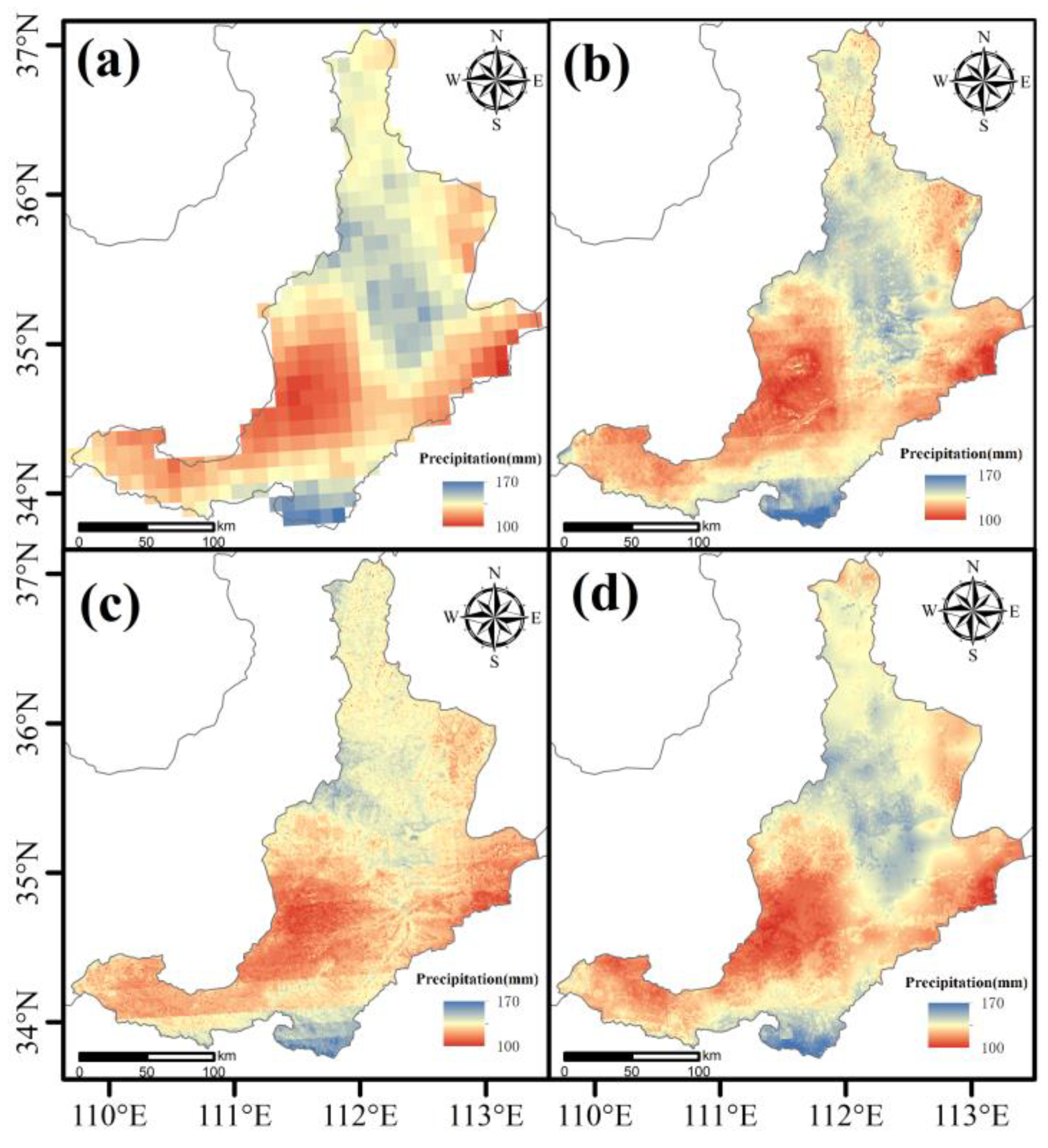
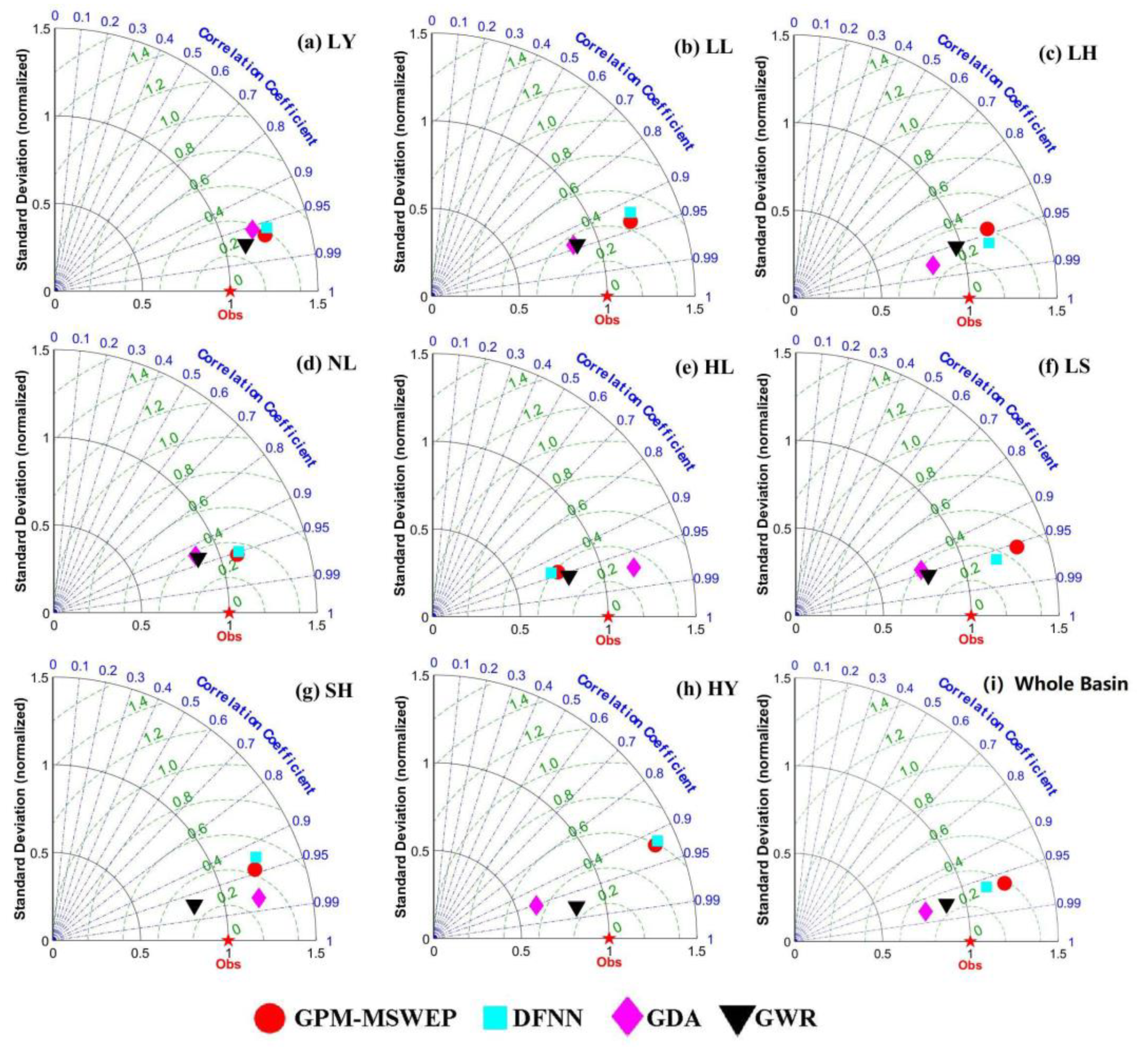
3.3. Calibration of Downscaled Results and Evaluation of Accuracy

Table 1. Precision assessment indices before and after downscaling calibration, combining monthly scale meteorological station data from 2001 to 2019.

	R2	RMSE (mm)	FSE	BIAS (%)
Original GPM-MSWEP	0.92	12.54	1.98	2.4
DFNN	0.92	12.77	1.92	1.4
GDA	0.93	12.03	1.93	1.0
GWR	0.93	12.00	1.90	0.5

shows the values of the four quantitative accuracy evaluation indicators (R², RMSE, FSE, and BIAS) for the original image, the DFNN-downscaled data, GDA calibration data, and GWR calibration data. As can be seen from the table, compared with the original satellite precipitation product, the simulation results of the DFNN downscaling model did not significantly improve the four accuracy evaluation indexes. The coefficient of determination R² remained flat at 0.92, the relative BIAS decreased from 2.4% to 1.4%, while the RMSE and the FSE rose slightly. This indicates that only considering the residual difference between simulated precipitation and original satellite precipitation cannot effectively improve the accuracy of downscaled data, so it is necessary to combine the actual precipitation on the ground for calibration. Compared with the original satellite precipitation product, the accuracy of downscaled data after GDA and GWR calibration was significantly improved. The GDA and GWR showed consistent superiority in four quantitative accuracy evaluation indexes, indicating that the calibration successfully solved the problem of overestimation in GPM-MSWEP data and improved its accuracy. Compared with the GDA calibration results, the GWR calibration results had a slight advantage in terms of the RMSE, FSE, and BIAS (RMSE = 12.00 mm, FSE = 1.90, BIAS = 0.5%). In general, the GWR calibration results were better than the GDA calibration results, and the four accuracy evaluation indexes were significantly improved. Compared to the original image, the R² increased from 0.92 to 0.93, the RMSE decreased from 12.54 mm to 12.00 mm, the FSE decreased from 1.98 to 1.90, and the BIAS decreased from 2.4% to 0.5%.

Figure 9 shows the values of the original image GPM-MSWEP, the DFNN-downscaled data, the GDA calibration data, and the GWR calibration data of four quantitative accuracy evaluation indexes (R², RMSE, FSE, and BIAS). The results show that in most months, the R² value of the downscaled data after GDA and GWR calibration was better than that of the original GPM-MSWEP data and the DFN-downscaled result. Before and after calibration, the corrected data showed small RMSE, FSE, and BIAS values, and the R² value remained stable. This shows that the calibration helped to improve the accuracy of the GPM-MSWEP monthly precipitation estimation results, and significantly reduced the deviation value. The downscaled results corrected using GWR exhibited the lowest RMSE, FSE, and BIAS, indicating that the DFNN had the most significant accuracy improvement effect after GWR calibration.

Figure 10 shows the eight regions of the Yellow River basin and the nine sets of Taylor charts of precipitation products in the Yellow River basin. Among all the sub-basins, the GWR data were closest to the meteorological station data in the SH region, while the DFNN data were furthest away from the meteorological station data in the LL region. In general, except for the LH and NL regions, the GWR-corrected DFNN-downscaled precipitation dataset performed best in all sub-basins, and its R² (0.865~0.952) increased by 0.014~0.021 compared with GPM-MSWEP (0.844~0.938). The surface downscaling calibration had a positive effect on the generation and release process of satellite remote sensing precipitation products, and the error calibration effect was good.

Figure 11 show the spatial distribution of errors between the GPM-MSWEP, DFNN, GDA, and GWR datasets and the meteorological station data in the Yellow River basin, respectively, in order to further compare the differences in the spatial distribution of the downscaled and corrected precipitation data obtained using downscaling correction methods for GPM-MSWEP. The R² of the GPM-MSWEP, DFNN, GDA, and GWR datasets reached above 0.85 in most areas, and the correlation was slightly lower in the northwestern LL sub-basin, while the RMSE of the four ranged from 4.71 to 31.95 mm, 6.10 to 32.62 mm, 3.18 to 31.20 mm, and 3.04 to 31.35 mm, respectively; the maximum FSE was 1.21~6.45, 1.47~7.01, 1.10~5.86, and 0.98~5.89, respectively, and the error performance in the eastern part of the basin was significantly improved after calibration in combination with the meteorological station data. In the northwestern part of the basin, there were significant deviations in the BIAS before calibration, and the maximum deviation range reached −32.8~43.4%. The calibration using GWR significantly improved the overestimation and underestimation of precipitation in the modified area. The above results show that the precipitation data corrected using GDA and GWR not only retained the spatial distribution characteristics of errors corresponding to the original satellite remote sensing precipitation products, but also the spatial distribution of errors over the whole basin were greatly improved. In addition, the accuracy of the corrected precipitation data was also improved, and the error control performance of the GWR-corrected precipitation data, in terms of the RMSE, FSE, and BIAS, were significantly better.

3.4. Stage Analysis and Spatial Trend Analysis

In Figure 12a, the blue line represents the actual precipitation after the smoothing process, while the red line indicates two mutation points, 2002 and 2016, in the period from 2001 to 2019. According to these points, the entire precipitation time series can be divided into three stages: 2001–2002, 2003–2016, and 2017–2019. This division helps reveal the characteristics of the precipitation in different time stages. From Figure 12b, the average precipitation values for the three stages were 414.22 mm, 463.15 mm, and 541.22 mm, respectively. The linear trend rates were 36.2 mm/year, 4.88 mm/year, and −69.0 mm/year, respectively. Figure 13a–h indicate that LY and LL experienced abrupt changes in 2002 and 2016, NL had changes in 2003 and 2016, LH in 2012, HL in 2011, and HY in 2002 and 2005. LS and SH underwent changes in 2002 and 2004. It can be observed that the abrupt changes in the annual precipitation series for most sub-basins were concentrated around the years 2002, 2004, and 2016, aligning with the timing of precipitation changes across the entire basin.

As shown in Figure 14 and Figure 15, it can be found that the trend characteristics of gridded precipitation in the Yellow River basin vary in different time periods. The mean values of Zs trend characteristics of precipitation in the Yellow River basin at the monthly scale were obtained as −0.17, 0.75, 0.28, 1.43, 0.25, 0.63, 0.51, 0.50, −0.20, 0.88, 0.89, and −0.89. Among them, the precipitation in three months (January, September, and December) showed a decreasing trend, while the precipitation in the other months exhibited an increasing trend. In April, August, October, and November, the mean Zs values of each sub-basin were greater than 0, indicating that the precipitation in these sub-basins had an increasing trend in these months; in December, except for LY, the mean Zs values of all sub-basins were less than 0, indicating that the precipitation in most sub-basins had a decreasing trend in December. The percentages of the area of the Yellow River basin with increasing precipitation in each month were 36.78%, 82.51%, 61.51%, 90.72%, 59.81%, 78.78%, 67.59%, 76.97%, 35.93%, 91.04%, 87.52%, and 15.03% of the total basin area, respectively.

On the seasonal scale, the mean Zs values of precipitation in the Yellow River basin in spring, summer, autumn, and winter were 1.23, 0.87, 0.66, and 0.13, respectively, indicating an increasing trend of precipitation in the spring, summer, autumn, and winter. Meanwhile, there was also variability in the quarterly precipitation trend characteristics in different sub-basins. The percentages of the area of the Yellow River basin with increasing precipitation trends in the spring, summer, autumn, and winter were 82.96%, 88.05%, 76.65%, and 55.86% of the total basin area, respectively. More than half of the grids had Zs trend eigenvalues greater than 0, indicating an overall increasing trend of precipitation in the Yellow River basin from 2001 to 2019.

4. Discussion

Based on the results of the suitability analysis, on the temporal scale, the R² values for GPM and MSWEP were 0.92 and 0.90, respectively, with the smallest RMSE and FSE, and the BIAS was close to 0. This indicates that the GPM and MSWEP datasets had higher accuracy, which is consistent with their performance observed in previous studies [44,45,46]. On the spatial scale, the CHIRPS, TRMM, and MSWEP datasets all showed similar spatial variability in terms of the RMSE and FSE, with lower values in the southeast and higher values in the northwest. The distribution of the RMSE and FSE for GPM data was more uniform, aligning with the conclusions regarding error variability found in previous research [47]. Based on the downscaling results, compared to the GBDT and RF, the DFNN was more capable of reflecting the differences in regional localized precipitation. This is because the traditional downscaling method downscales the low-resolution pixels of the original image one by one, resulting in the downscaled result preserving the approximate precipitation at the low-resolution pixel boundary of the original image [48]. At the same time, when the regression model is constructed using CART and other algorithms, the discontinuity of its prediction surface leads to the non-smooth transition of simulation results [49]; in particular, when precipitation with spatial continuity is simulated, the limitations of the algorithm seriously affect the accuracy. RF and GBDT are extensions of the CART algorithm. The downscaled results are also affected by the discontinuity characteristics of the CART algorithm, and pixel boundaries appear when simulating the spatial distribution of precipitation. DFNN is a method based on deep learning. Unlike other regression tree algorithms, its basic unit uses continuous nonlinear functions and is differentiable, at least in decimal places, to ensure the smoothness of precipitation estimation across the study area [50]. Based on the calibration results, all four evaluation indicators of GWR (R² = 0.93, RMSE = 12.00 mm, FSE = 1.90, BIAS = 0.5%) were superior to those of GDA. Moreover, GWR showed a significant advantage over GDA in the calibration effects across most months and sub-basins. This may be because the parameters of traditional econometric models are constant in global space, while GWR allows for variable parameters within global space. This enables a better description of the relationship between independent and dependent variables as they change across space, which is also consistent with previous research [51].

There are also some limitations in this study. In the downscaling method of this study, the selection of explanatory variables was relatively conservative. Due to the complex terrain of the Yellow River basin, the same explanatory variables have different impacts on precipitation in different geographical units. Future research could consider introducing corresponding independent variables under different climate and topographic conditions, such as sunshine duration, temperature, and water vapor, to compare the impact of adding other explanatory variables on the accuracy of model output results. It could also study the weights of explanatory variables in different geographical units more meticulously, thereby constructing a downscaling model that is more suitable for a certain region and obtaining more accurate meteorological element data. Despite the limitations, this study resolved the problem of the non-smooth transition of precipitation in traditional downscaling results and obtained high-resolution spatial data and high-accuracy precipitation results in the long time-series of the Yellow River basin. This supplements the surface continuous precipitation data for the Yellow River basin, which is unevenly distributed with meteorological stations, and lays the foundation for future research.

5. Conclusions

This study focused on the Yellow River basin as the research area, evaluating the GPM, MSWEP, TRMM, and CHIRPS to construct high-precision optimal combination products. The study employed DFNN, GBDT, and RF for downscaling, calibrated based on meteorological station data, and analyzed the spatiotemporal trends of precipitation. The main conclusions of this study are as follows.

(1)

On the temporal scale, GPM and MSWEP had the highest accuracy in the Yellow River basin, with R² values of 0.92 and 0.90, respectively, and the smallest RMSE and FSE, with a BIAS close to 0. The TRMM and CHIRPS had the lowest accuracy. On the spatial scale, GPM had a better distribution of R² and the smallest BIAS. The optimal combination of GPM and MSWEP was selected to construct a high-precision mixed dataset.

(2)

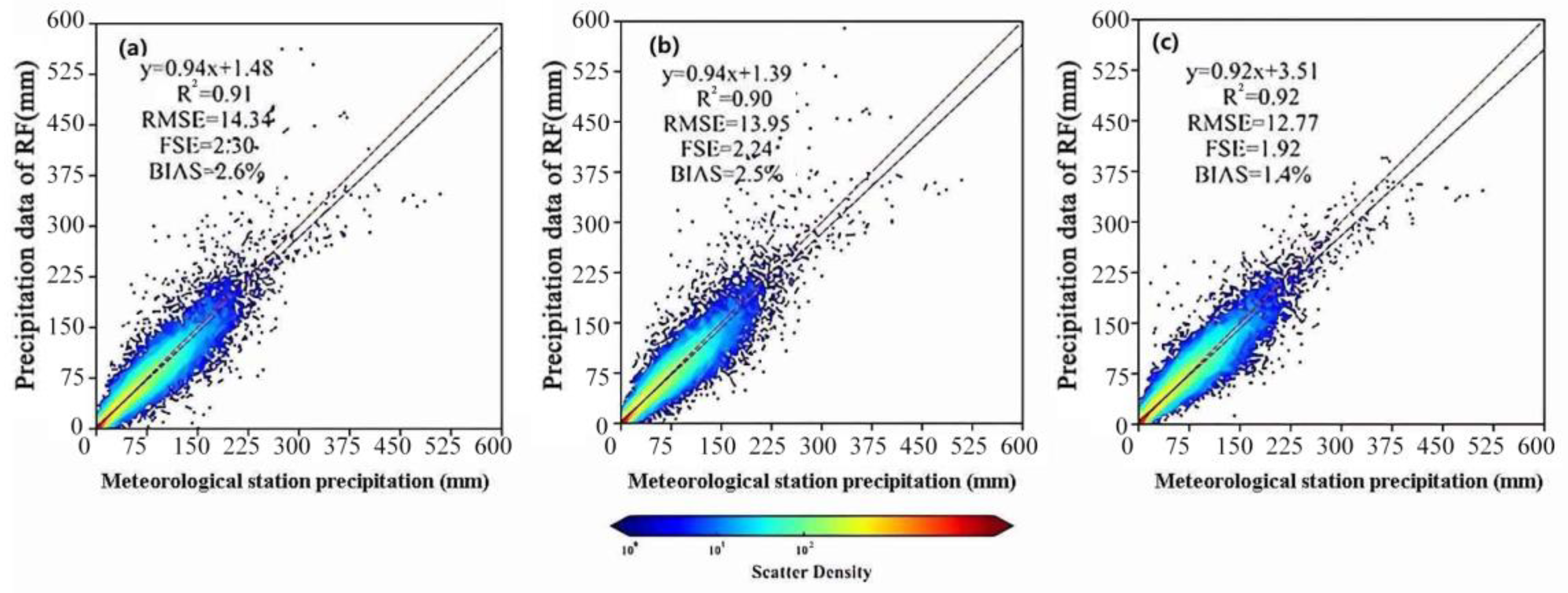
The DFNN downscaling results displayed better spatial details, more accurately reflecting the differences in regional localized precipitation. DFNN had a higher R² and lower RMSE, FSE, and BIAS (R² = 0.92, RMSE = 12.77, FSE = 1.92, BIAS = 1.4%), demonstrating better error control.

(3)

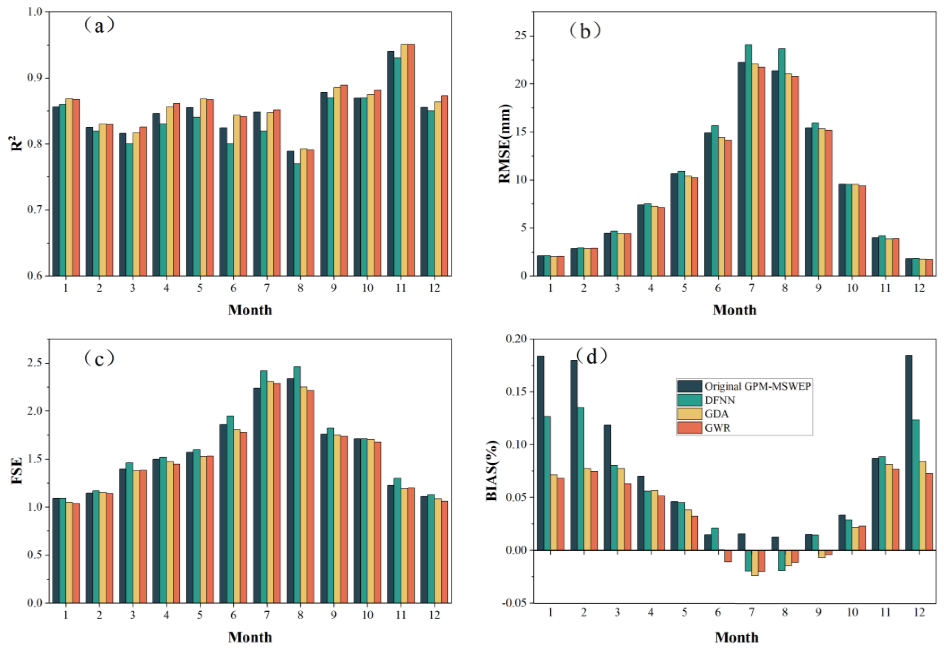
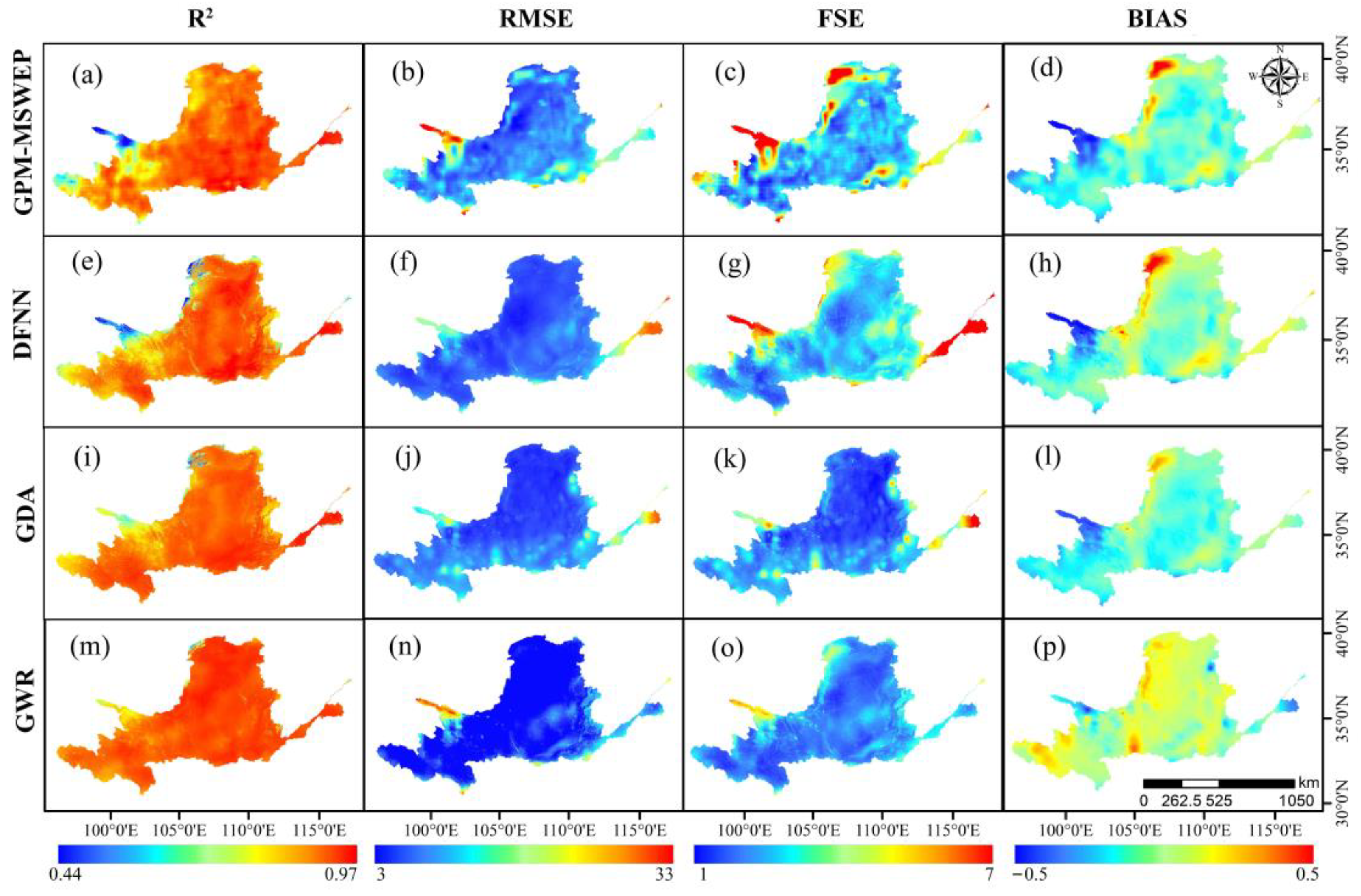
After calibration with GWR and GDA, the data accuracy was improved, and GWR’s calibration effect was superior to that of the GDA. After GWR calibration, the DFNN downscaling results saw an increase in R² from 0.92 to 0.93, a decrease in RMSE from 12.77 to 12.00 mm, a decrease in FSE from 1.92 to 1.90, and a decrease in BIAS from 1.4% to 0.5%.

(4)

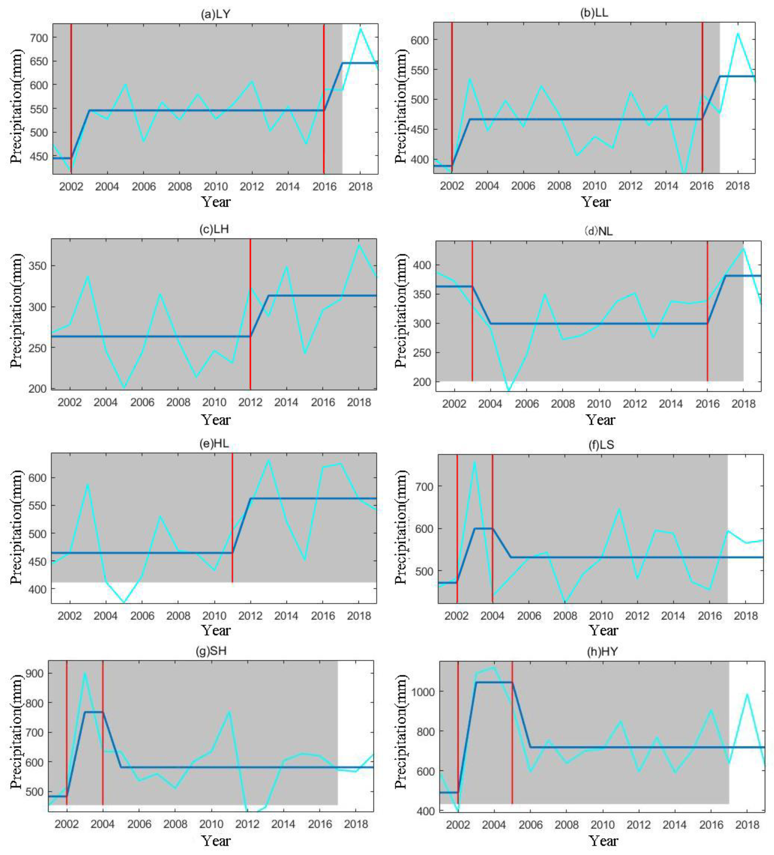
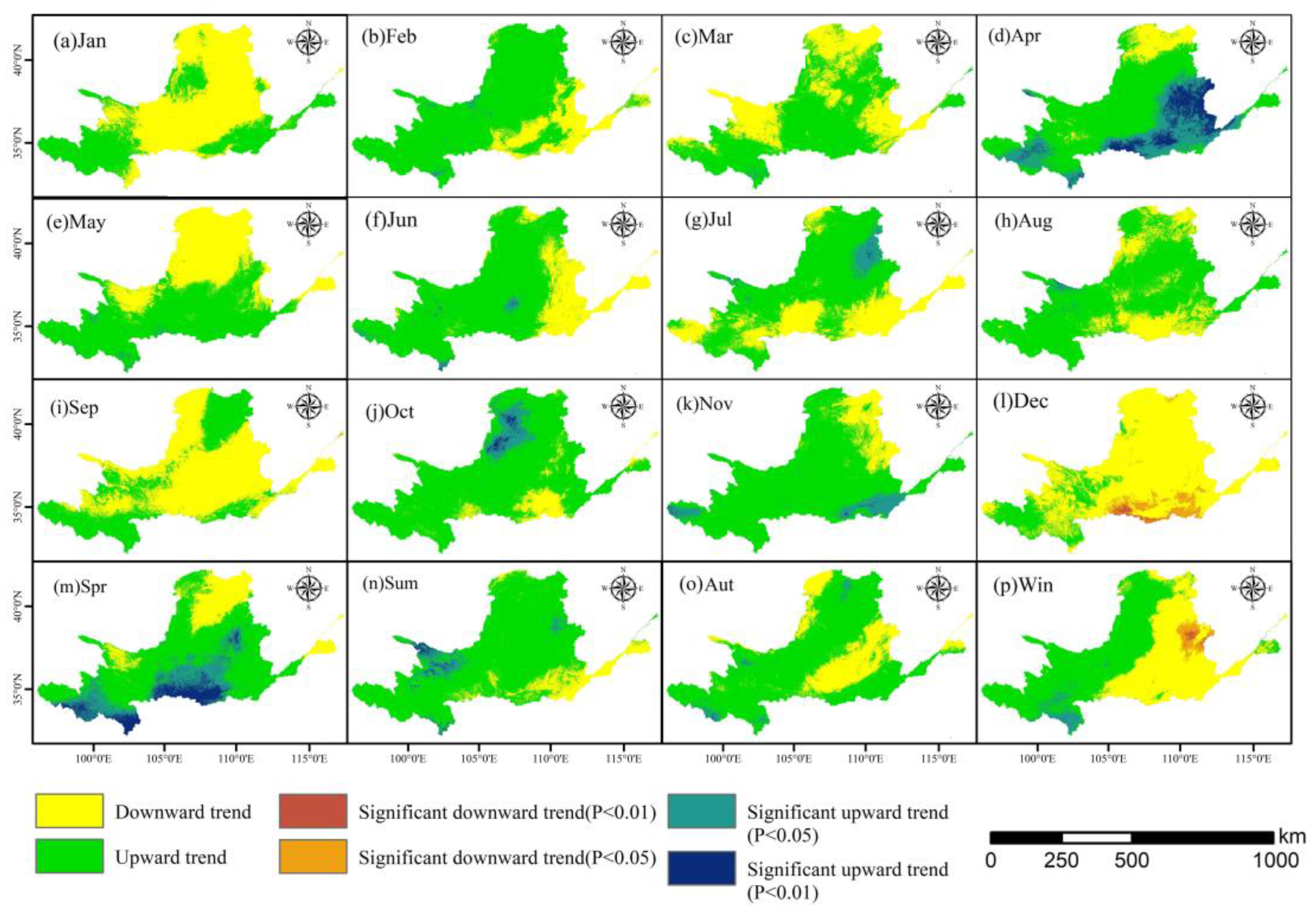
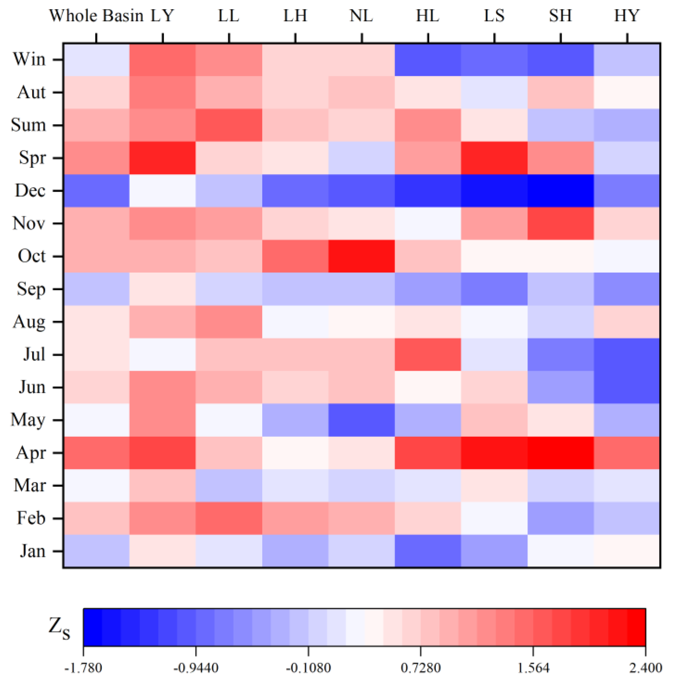
There were two abrupt changes in annual precipitation in the Yellow River basin in 2002 and 2016. On the monthly scale, the precipitation in January, September, and December showed a decreasing trend, and the precipitation in the remaining months showed an increasing trend. On the seasonal scale, the precipitation in spring, summer, fall, and winter showed an increasing trend.

References

1. Huffman, G.J.; Bolvin, D.T.; Nelkin, E.J.; Wolff, D.B.; Adler, R.F.; Gu, G.; Hong, Y.; Bowman, K.P.; Stocker, E.F. The TRMM multisatellite precipitation analysis (TMPA): Quasi-global, multiyear, combined-sensor precipitation estimates at fine scales. J. Hydrometeorol. 2007, 8, 38–55. [Google Scholar] [CrossRef]
2. Kubota, T.; Shige, S.; Hashizume, H.; Aonashi, K.; Takahashi, N.; Seto, S.; Hirose, M.; Takayabu, Y.N.; Ushio, T.; Nakagawa, K. Global precipitation map using satellite-borne microwave radiometers by the GSMaP project: Production and validation. IEEE Trans. Geosci. Remote Sens. 2007, 45, 2259–2275. [Google Scholar] [CrossRef]
3. Funk, C.; Peterson, P.; Landsfeld, M.; Pedreros, D.; Verdin, J.; Shukla, S.; Husak, G.; Rowland, J.; Harrison, L.; Hoell, A. The climate hazards infrared precipitation with stations—A new environmental record for monitoring extremes. Sci. Data 2015, 2, 150066. [Google Scholar] [CrossRef] [PubMed]
4. Funk, C.; Verdin, A.; Michaelsen, J.; Peterson, P.; Pedreros, D.; Husak, G. A global satellite-assisted precipitation climatology. Earth Syst. Sci. Data 2015, 7, 275–287. [Google Scholar]
5. Li, Z.; Yang, D.; Gao, B.; Jiao, Y.; Hong, Y.; Xu, T. Multiscale hydrologic applications of the latest satellite precipitation products in the Yangtze River Basin using a distributed hydrologic model. J. Hydrometeorol. 2015, 16, 407–426. [Google Scholar] [CrossRef]
6. Duan, Z.; Liu, J.; Tuo, Y.; Chiogna, G.; Disse, M. Evaluation of eight high spatial resolution gridded precipitation products in Adige Basin (Italy) at multiple temporal and spatial scales. Sci. Total Environ. 2016, 573, 1536–1553. [Google Scholar] [CrossRef]
7. Lu, D.; Yong, B. A preliminary assessment of the gauge-adjusted near-real-time GSMaP precipitation estimate over Mainland China. Remote Sens. 2020, 12, 141. [Google Scholar] [CrossRef]
8. Islam, M.A.; Yu, B.; Cartwright, N. Assessment and comparison of five satellite precipitation products in Australia. J. Hydrol. 2020, 590, 125474. [Google Scholar] [CrossRef]
9. Aslami, F.; Ghorbani, A.; Sobhani, B.; Esmali, A. Comprehensive comparison of daily IMERG and GSMaP satellite precipitation products in Ardabil Province, Iran. Int. J. Remote Sens. 2019, 40, 3139–3153. [Google Scholar] [CrossRef]
10. Yu, C.; Hu, D.; Liu, M.; Wang, S.; Di, Y. Spatio-temporal accuracy evaluation of three high-resolution satellite precipitation products in China area. Atmos. Res. 2020, 241, 104952. [Google Scholar] [CrossRef]
11. McCollum, J.R.; Krajewski, W.F.; Ferraro, R.R.; Ba, M.B. Evaluation of BIASes of satellite rainfall estimation algorithms over the continental United States. J. Appl. Meteorol. Climatol. 2002, 41, 1065–1080. [Google Scholar] [CrossRef]
12. Tang, G.; Ma, Y.; Long, D.; Zhong, L.; Hong, Y. Evaluation of GPM Day-1 IMERG and TMPA Version-7 legacy products over Mainland China at multiple spatiotemporal scales. J. Hydrol. 2016, 533, 152–167. [Google Scholar] [CrossRef]
13. Sa’adi, Z.; Shahid, S.; Chung, E.-S.; bin Ismail, T. Projection of spatial and temporal changes of rainfall in Sarawak of Borneo Island using statistical downscaling of CMIP5 models. Atmos. Res. 2017, 197, 446–460. [Google Scholar] [CrossRef]
14. Wu, X.; Zhao, N. Evaluation and Comparison of Six High-Resolution Daily Precipitation Products in Mainland China. Remote Sens. 2022, 15, 223. [Google Scholar] [CrossRef]
15. Atkinson, P.M. Downscaling in remote sensing. Int. J. Appl. Earth Obs. Geoinf. 2013, 22, 106–114. [Google Scholar] [CrossRef]
16. Legasa, M.; Manzanas, R.; Calviño, A.; Gutiérrez, J.M. A posteriori random forests for stochastic downscaling of precipitation by predicting probability distributions. Water Resour. Res. 2022, 58, e2021WR030272. [Google Scholar] [CrossRef]
17. Wilby, R.L.; Wigley, T. Precipitation predictors for downscaling: Observed and general circulation model relationships. Int. J. Climatol. A J. R. Meteorol. Soc. 2000, 20, 641–661. [Google Scholar] [CrossRef]
18. Chen, T.; Guestrin, C. Xgboost: A scalable tree boosting system. In Proceedings of the 22nd Acm Sigkdd International Conference on Knowledge Discovery and Data Mining, San Francisco, CA, USA, 13–17 August 2016; pp. 785–794. [Google Scholar]
19. Chen, W.; Fu, K.; Zuo, J.; Zheng, X.; Huang, T.; Ren, W. Radar emitter classification for large data set based on weighted-xgboost. IET Radar Sonar Navig. 2017, 11, 1203–1207. [Google Scholar] [CrossRef]
20. Liu, J.; Zhang, W.; Nie, N. Spatial downscaling of TRMM precipitation data using an optimal subset regression model with NDVI and terrain factors in the Yarlung Zangbo River Basin, China. Adv. Meteorol. 2018, 2018, 1–13. [Google Scholar] [CrossRef]
21. Mao, K.; Tang, H.; Wang, X.; Zhou, Q.; Wang, D. Near-surface air temperature estimation from ASTER data based on neural network algorithm. Int. J. Remote Sens. 2008, 29, 6021–6028. [Google Scholar] [CrossRef]
22. Wu, Y.; Zhang, Z.; Crabbe, M.J.C.; Chandra Das, L. Statistical learning-based spatial downscaling models for precipitation distribution. Adv. Meteorol. 2022, 2022, 3140872. [Google Scholar] [CrossRef]
23. Xu, R.; Chen, N.; Chen, Y.; Chen, Z. Downscaling and projection of multi-cmip5 precipitation using machine learning methods in the upper han river Basin. Adv. Meteorol. 2020, 2020, 8680436. [Google Scholar] [CrossRef]
24. Ridgeway, G. Additive logistic regression: A statistical view of boosting: Discussion. Ann. Stat. 2000, 28, 393–400. [Google Scholar]
25. Wager, S. Asymptotic theory for random forests. arXiv 2014, arXiv:1405.0352. [Google Scholar]
26. Maji, D.; Santara, A.; Ghosh, S.; Sheet, D.; Mitra, P. Deep neural network and random forest hybrid architecture for learning to detect retinal vessels in fundus images. In Proceedings of the 2015 37th Annual International Conference of the IEEE Engineering in Medicine and Biology Society (EMBC), Milan, Italy, 25–29 August 2015; IEEE: Piscataway, NJ, USA, 2015. [Google Scholar]
27. Ha, V.K.; Ren, J.; Xu, X.; Zhao, S.; Xie, G.; Vargas, V.M. Deep learning based single image super-resolution: A survey. In Proceedings of the Advances in Brain Inspired Cognitive Systems: 9th International Conference, BICS 2018, Xi’an, China, 7–8 July 2018; Springer: Berlin, Germany, 2018. [Google Scholar]
28. Baez-Villanueva, O.M.; Zambrano-Bigiarini, M.; Beck, H.E.; McNamara, I.; Ribbe, L.; Nauditt, A.; Birkel, C.; Verbist, K.; Giraldo-Osorio, J.D.; Thinh, N.X. RF-MEP: A novel Random Forest method for merging gridded precipitation products and ground-based measurements. Remote Sens. Environ. 2020, 239, 111606. [Google Scholar] [CrossRef]
29. Cheema, M.J.M.; Bastiaanssen, W.G. Local calibration of remotely sensed rainfall from the TRMM satellite for different periods and spatial scales in the Indus Basin. Int. J. Remote Sens. 2012, 33, 2603–2627. [Google Scholar] [CrossRef]
30. Duan, Z.; Bastiaanssen, W. First results from Version 7 TRMM 3B43 precipitation product in combination with a new downscaling–calibration procedure. Remote Sens. Environ. 2013, 131, 1–13. [Google Scholar] [CrossRef]
31. Yu, H.; Wang, L.; Yang, R.; Yang, M.; Gao, R. Temporal and spatial variation of precipitation in the Hengduan Mountains region in China and its relationship with elevation and latitude. Atmos. Res. 2018, 213, 1–16. [Google Scholar] [CrossRef]
32. Khan, M.; Munoz-Arriola, F.; Rehana, S.; Greer, P. Spatial heterogeneity of temporal shifts in extreme precipitation across India. J. Clim. Chang. 2019, 5, 19–31. [Google Scholar] [CrossRef]
33. Breiman, L. Bagging predictors. Mach. Learn. 1996, 24, 123–140. [Google Scholar] [CrossRef]
34. Breiman, L. Classification and Regression Trees; Routledge: London, UK, 2017. [Google Scholar]
35. Carlisle, D.M.; Falcone, J.; Wolock, D.M.; Meador, M.R.; Norris, R.H. Predicting the natural flow regime: Models for assessing hydrological alteration in streams. River Res. Appl. 2010, 26, 118–136. [Google Scholar] [CrossRef]
36. Chaney, N.W.; Wood, E.F.; McBratney, A.B.; Hempel, J.W.; Nauman, T.W.; Brungard, C.W.; Odgers, N.P. POLARIS: A 30-meter probabilistic soil series map of the contiguous United States. Geoderma 2016, 274, 54–67. [Google Scholar] [CrossRef]
37. Catani, F.; Lagomarsino, D.; Segoni, S.; Tofani, V. Landslide susceptibility estimation by random forests technique: Sensitivity and scaling issues. Nat. Hazards Earth Syst. Sci. 2013, 13, 2815–2831. [Google Scholar] [CrossRef]
38. Friedman, J.; Hastie, T.; Tibshirani, R. Additive logistic regression: A statistical view of boosting (with discussion and a rejoinder by the authors). Ann. Stat. 2000, 28, 337–407. [Google Scholar] [CrossRef]
39. Zhang, D.; Zhang, W.; Huang, W.; Hong, Z.; Meng, L. Upscaling of surface soil moisture using a deep learning model with VIIRS RDR. ISPRS Int. J. Geo-Inf. 2017, 6, 130. [Google Scholar] [CrossRef]
40. Brunsdon, C.; Fotheringham, A.S.; Charlton, M. Spatial nonstationarity and autoregressive models. Environ. Plan. A 1998, 30, 957–973. [Google Scholar] [CrossRef]
41. Bernaola-Galván, P.; Ivanov, P.C.; Amaral, L.A.N.; Stanley, H.E. Scale invariance in the nonstationarity of human heart rate. Phys. Rev. Lett. 2001, 87, 168105. [Google Scholar] [CrossRef] [PubMed]
42. Mann, H.B. Nonparametric tests against trend. Econom. J. Econom. Soc. 1945, 13, 245–259. [Google Scholar] [CrossRef]
43. Hamed, K.H.; Rao, A.R. A modified Mann-Kendall trend test for autocorrelated data. J. Hydrol. 1998, 204, 182–196. [Google Scholar] [CrossRef]
44. Hamza, A.; Anjum, M.N.; Masud Cheema, M.J.; Chen, X.; Afzal, A.; Azam, M.; Kamran Shafi, M.; Gulakhmadov, A. Assessment of IMERG-V06, TRMM-3B42V7, SM2RAIN-ASCAT, and PERSIANN-CDR precipitation products over the Hindu Kush Mountains of Pakistan, South Asia. Remote Sens. 2020, 12, 3871. [Google Scholar] [CrossRef]
45. Sharifi, E.; Saghafian, B.; Steinacker, R. Downscaling satellite precipitation estimates with multiple linear regression, artificial neural networks, and spline interpolation techniques. J. Geophys. Res. Atmos. 2019, 124, 789–805. [Google Scholar] [CrossRef]
46. Beck, H.E.; Van Dijk, A.I.; Levizzani, V.; Schellekens, J.; Miralles, D.G.; Martens, B.; De Roo, A. MSWEP: 3-hourly 0.25 global gridded precipitation (1979–2015) by merging gauge, satellite, and reanalysis data. Hydrol. Earth Syst. Sci. 2017, 21, 589–615. [Google Scholar] [CrossRef]
47. Zhao, C.; Ren, L.; Yuan, F.; Zhang, L.; Jiang, S.; Shi, J.; Chen, T.; Liu, S.; Yang, X.; Liu, Y. Statistical and hydrological evaluations of multiple satellite precipitation products in the yellow river source region of china. Water 2020, 12, 3082. [Google Scholar] [CrossRef]
48. Chen, S.; Zhang, L.; She, D.; Chen, J. Spatial downscaling of tropical rainfall measuring mission (TRMM) annual and monthly precipitation data over the middle and lower reaches of the Yangtze River Basin, China. Water 2019, 11, 568. [Google Scholar] [CrossRef]
49. Hastie, T.; Tibshirani, R.; Friedman, J.H.; Friedman, J.H. The Elements of Statistical Learning: Data Mining, Inference, and Prediction; Springer: Berlin, Germany, 2009; Volume 2. [Google Scholar]
50. Tao, Y.; Gao, X.; Hsu, K.; Sorooshian, S.; Ihler, A. A deep neural network modeling framework to reduce BIAS in satellite precipitation products. J. Hydrometeorol. 2016, 17, 931–945. [Google Scholar] [CrossRef]
51. Chen, Y.; Huang, J.; Sheng, S.; Mansaray, L.R.; Liu, Z.; Wu, H.; Wang, X. A new downscaling-integration framework for high-resolution monthly precipitation estimates: Combining rain gauge observations, satellite-derived precipitation data and geographical ancillary data. Remote Sens. Environ. 2018, 214, 154–172. [Google Scholar] [CrossRef]
Figure 1. Study area.
Remotesensing 16 01318 g001
Figure 2. Flowchart of the research.
Remotesensing 16 01318 g002
Figure 3. Monthly scale scatter plots of meteorological station data from 2001 to 2019 with four types of satellite remote sensing precipitation products, (a) CHIRPS; (b) TRMM; (c) MSWEP; (d) GPM.
Remotesensing 16 01318 g003
Figure 4. Spatial distribution of evaluation indicators for four types of satellite remote sensing precipitation products from 2001 to 2019, (ad) CHIRPS; (eh) TRMM; (il) MSWEP; (mp)GPM.
Remotesensing 16 01318 g004
Figure 5. Comparison of monthly accuracy of precipitation satellite data. The horizontal coordinate represents the accuracy of each precipitation satellite data. The ordinate is an acronym for the month.
Remotesensing 16 01318 g005
Figure 6. Downscaled results for Yellow River basin in July 2012: (ac) predicted precipitation of RF, GBDT, and DFNN; (df) downscaled residuals of RF, GBDT, and DFNN; (gi) downscaled results of RF, GBDT, and DFNN; (j) low-resolution raw image.
Remotesensing 16 01318 g006
Figure 7. Downscaled results of SH sub-basin in July 2012: (a) low-resolution raw image, (b) downscaled results of RF, (c) downscaled results of GBDT, (d) downscaled results of DFNN.
Remotesensing 16 01318 g007
Figure 8. Monthly scale scatterplots of meteorological precipitation station data from 2001 to 2019 with three downscaling results: (a) RF; (b) GBD; (c) DFNN.
Remotesensing 16 01318 g008
Figure 9. Validation results of the original GPM-MSWEP data, downscaled data based on DNFF algorithm, downscaled data based on GDA calibration, and downscaled data based on GWR calibration using meteorological station data of the Yellow River basin from 2001 to 2019: (a) R2; (b) RMSE; (c) FSE; (d) BIAS.
Remotesensing 16 01318 g009
Figure 10. Taylor diagram of precipitation dataset before and after downscaling calibration in the Yellow River basin and eight sub-basins.
Remotesensing 16 01318 g010
Figure 11. Spatial distribution of evaluation indicators for downscaled corrected precipitation data from 2001 to 2019: (ad) GPM-MSWEP; (eh) DFNN; (il) GDA; (mp) GWR.
Remotesensing 16 01318 g011
Figure 12. Stage characteristics of precipitation in the Yellow River basin from 2001 to 2019: (a) detection of sudden changes in annual precipitation; (b) trends in annual precipitation at different time stages.
Remotesensing 16 01318 g012
Figure 13. Stage characteristics of precipitation in sub-basins of the Yellow River basin from 2001 to 2019.
Remotesensing 16 01318 g013
Figure 14. Trend characteristics of gridded precipitation in the Yellow River basin from 2001 to 2019: (al) Jan–Dec; (mp) Spr–Win.
Remotesensing 16 01318 g014
Figure 15. Trend characteristic Zs values of precipitation in the Yellow River basin and its sub-basins from 2001 to2019.
Remotesensing 16 01318 g015