Impact of Channel Selection with Different Bandwidths on Retrieval at 50–60 GHz

Abstract

Microwave hyperspectral instruments represent one of the main atmospheric sounders of China’s next-generation Fengyun meteorological satellites. In order to better apply microwave hyperspectral observations in the fields of atmospheric parameter retrieval and data assimilation, this paper analyzes the sensitivity of trace gases to five selected bandwidth channels using a radiative transfer model based on the simulated data of microwave hyperspectral radiances at 50–60 GHz. This method uses information entropy and a weighting function to select channels and analyze the impact of this on the retrieval accuracy of atmospheric profiles before and after channel selection. The experimental results show that channel selection can reduce the number of channels by approximately 74.05% while maintaining a large amount of information content, and this retrieval effect is significantly better than that of MWTS-III. After channel selection, the 10 MHz, 30 MHz, and 50 MHz bandwidths have the best retrieval results in the stratosphere, whole atmosphere, and troposphere, respectively. When considering the number of channels, computational scale, and retrieval results comprehensively, the channel selection method is effective.

1. Introduction

Temperature is an important physical parameter of the atmosphere that can characterize the thermal state of the atmosphere and determine its thermodynamic processes. The effective detection of atmospheric temperature profiles in real time is useful for describing atmospheric evolution, monitoring the climate, and evaluating numerical weather prediction models, and it is equally important for other meteorological protection work [1]. Meteorological satellite observations have the advantages of greater information content, wide coverage, and high spatiotemporal resolution. In areas where conventional data are difficult to observe, satellite observations are particularly important. In recent years, with the development of multi-channel meteorological satellites and the continuous improvement of grid resolution in weather prediction models, hyperspectral sounders with high spatiotemporal resolution and high spectral resolution have been widely developed and applied [2,3]. With the use of sounders such as the infrared atmospheric sounding interferometer (IASI) onboard MetOp, the atmospheric infrared sounder (AIRS) onboard Aqua, the cross-track infrared sounder (CrIS) onboard SNPP, and the high spectral resolution infrared atmospheric sounder (HIRAS) onboard FY-3D/E, atmospheric sounding has been greatly improved by hyperspectral measurements, which yield greater vertical resolution throughout the atmosphere. The atmospheric thermodynamic parameters obtained by infrared hyperspectral sounders can effectively invert atmospheric parameters and are an important source of data for climate studies [4,5,6,7].

Although infrared has been applied to the detection of temperature profiles, observations in the microwave spectrum can sound atmospheric temperature and humidity information below thin clouds and retrieve weather structures [8]. Therefore, it is very important to use microwave sounders to detect the atmospheric profile, which can make up for the shortcomings of other means of atmospheric detection. In order to obtain more detailed information about the atmosphere and improve the atmospheric detection accuracy of microwave sounders, the application of hyperspectral technology in microwave sounders is an inevitable trend. Microwave sounders have been developed since the 1960s, initially with a small number of channels. With the continuous development of research and technology, microwave sounders are gradually moving towards increasing the number of channels, reducing volume, and reducing power consumption. In 1998, AMSU, which had more sounding channels and a higher spatial resolution, was launched so that the temperature distribution at high altitudes could be obtained by channels close to strong oxygen absorption lines [9]. The Microwave Temperature Sounder-III (MWTS-III) onboard the FY-3E satellite and the microwave sounder (MWS) of the European Meteorological Satellite (EUMETSAT) refine the sounding channels at 53 GHz [10]. In theory, using hyperspectral microwave sounders to detect the atmosphere can improve the detection accuracy compared to ordinary microwave sounders while positively impacting atmospheric retrieval.

The microwave absorption spectrum of oxygen has a clear frequency partition, with absorption lines mainly located at 118.75 GHz and 50–70 GHz, and these two absorption bands can be used to detect the atmospheric temperature profile. The results show that the detection channel located in the absorption band of 118 GHz has a certain ability to detect the vertical distribution of temperature, but it is more seriously affected by precipitation; the perturbation of 118 GHz by clouds and precipitation is twice as much as that of 60 GHz [11,12]. Therefore, the 50–60 GHz band can be selected as the detection band for atmospheric temperature profiles, and the microwave fine spectrum detection of future meteorological satellites mainly seeks to finely divide this frequency band and improve the vertical resolution of detection [13]. Therefore, the application of hyperspectral technology at 50–60 GHz is very worthy of study.

Microwave sounders can obtain more detection information, but at the same time, this also means more noise and a larger computational scale for assimilation prediction. Therefore, it is necessary to analyze the relevant methods of channel selection. In this paper, based on the simulated microwave hyperspectral radiances, we analyze the information content, weighting function, channel bandwidth, and other information of channels at 50–60 GHz at different bandwidths; this allows us to obtain appropriate channels and demonstrate their effects before and after channel selection via the retrieval results. The remainder of this paper is organized as follows: Section 2 introduces the channel-selection methods and radiative transfer model, Section 3 introduces the channel-selection experiments, Section 4 introduces the retrieval results, and the conclusion is presented in Section 5.

2. Method and Model

2.1. Channel Selection Algorithm

Information entropy can measure the uncertainty of the information source, so many scholars have applied this method to hyperspectral channel selection. The method we used for channel selection is the one suggested by Rodgers, which relies on evaluating the impact of the single channel on a figure of merit [14]. In this paper, entropy reduction (ER) is chosen for channel selection, which focuses on selecting the channels that have the greatest impact on information entropy [15].

Channel selection using the information entropy method is mainly based on Equation (1):

$$A_i=A_{i-1}(I-\frac{h_i{\left(A_{i-1}{h}_i\right)}^T}{1+{\left(A_{i-1}{h}_i\right)}^T{h}_i})$$

(1)

where $A_i$ is the analysis error covariance matrix after selecting i channels. When i = 0, $A_0$ = B, and B is the background error covariance matrix. $h_i$ is the vector corresponding to a line in $H^{\prime }$. The normalization of the Jacobian matrix is defined by Equation (2):

$$H^{\prime }=R^{-1/2}H$$

(2)

where R denotes the measurement error covariance matrix, which generally includes the observation error and the forward modeling error.

Some useful information theory concepts can be used to quantify the gain in information brought by data. In particular, we used ER method:

$$ER=-\frac{1}{2}{log}_{2}det\left(A_i{B}^{-1}\right)$$

(3)

where det denotes the determinant [16].

By using the ER method for channel selection, we selected the channel corresponding to the maximum value of ER in each iteration and then used the unselected channels in this iteration process as the candidate channels for the next iteration. Finally, when the entropy change was no longer significant, the iteration stopped, and the selected channel set was obtained. In the channel selection method of information entropy, the calculation of ER depends on the background error covariance matrix and analysis error covariance matrix. In the first iteration, the computation of the analysis error covariance matrix also depends on the given background error covariance matrix. In this paper, the background error covariance is based on the statistical results of global samples [17].

After channel selection using the ER method, further selection is required based on the weighting function. The weighting function represents the radiation contribution of the atmosphere to the satellite instruments at different altitudes in different bands. The ideal weighting function of the channel should only have a single peak. If there are multiple peaks, it indicates that the detection height of the channel is not unique. Therefore, channels with multiple peaks in the weighting function will be prioritized for elimination during channel selection. In order to obtain high vertical resolution data, the detection height of the selected channel set should cover as many height layers as possible. Among the channels with the same detection height, the channel with the largest peak value of the weighting function is selected [18]. This channel selection method ensures that a large amount of information content is retained while reducing the number of channels.

2.2. Radiative Transfer Simulation Model

Atmospheric Radiative Transfer Simulator (ARTS) is a modular program, and it is a relatively general and flexible model. ARTS can simulate brightness temperatures in microwave hyperspectral bands, calculate the absorption coefficient, calculate the Jacobian matrix, and more [19]. ARTS can perform line-by-line absorption calculations to calculate the absorption coefficient, but it also includes some predefined complete absorption models. The absorption can be calculated explicitly for each position along the propagation path, which gives the highest possible accuracy [20].

The absorption coefficient $\alpha$, as defined by Equation (4), is

$$\alpha \left(v,p,T,x_1,\dots ,x_n\right)=\begin{array}{c}\sum _{i=1}^N\frac{p{X}_i}{K_{B}T}\sum _{j=1}^{M_i}{S}_{ij}\left(T\right)F\left({\tilde{v}}_{ij},v,p,T,x_1,\dots ,x_n\right)\hfill \\ +C_1(v,p,T,x_1,\dots ,x_n)+\dots +C_L\left(v,p,T,x_1,\dots ,x_n\right)\hfill \end{array}$$

(4)

where v is the frequency, T is the temperature, p is the pressure, and $x_1,\dots ,x_n$ are the volume-mixing ratios of the various gas species. The index i goes over all N gas species, and the index j covers the overall $M_i$ spectral lines of each gas species. $K_B$ is Boltzmann’s constant, which means that this term is nothing other than the partial density, $n_i$, of a gas species, i. The contribution of each spectral line is given by the product of the line intensity, $S_{ij}\left(T\right)$, and the line shape function, $F({\tilde{v}}_{ij},\dots )$, and ${\tilde{v}}_{ij}$ is the line center frequency. $C_1$ to $C_L$ represent the functions of frequency, pressure, temperature, and gas volume-mixing ratios.

The atmospheric radiative transfer model ARTS uses a Jacobian matrix calculation with the following mathematical Equation (5):

$$K_x=\frac{\partial y}{\partial x_i}$$

(5)

where y refers to the brightness temperature $T_B$, and $x_i$ refers to the atmospheric state variables in layer i. The mathematical significance of the Jacobian matrix is the sensitivity of the brightness temperature to the state variables. This may be calculated by either using the perturbation method or semi-analytical approach. In order to improve the speed of computation, this paper uses the semi-analytical approach.

In the semi-analytical approach, it is possible to derive analytical expressions for the Jacobian for some atmospheric variables:

$$K_p=H\frac{\partial i}{\partial x_p}=H\left[\frac{\partial i}{\partial {\beta }_p}\frac{\partial {\beta }_p}{\partial x_p}+\frac{\partial i}{\partial a_p}\frac{\partial a_p}{\partial x_p}\right]$$

(6)

where $K_p$ is column p of the K matrix, and ${\beta }_p$ and $a_p$ are the Planck function and total absorption, respectively, at the vertical altitude corresponding to $x_p$. i is the vector holding monochromatic pencil beam spectral values, and H is the response matrix [19,21].

The atmospheric profile dataset used for the simulation studies in this paper was obtained from the European Centre for Medium-Range Weather Forecasts (ECMWF) Numerical Weather Prediction (NWP) global model. The profiles are given in a 137-level vertical grid, extending from the surface up to 0.01 hPa [22].

3. Channel Selection Experiments

3.1. Experimental Design

When conducting channel selections for microwave hyperspectral instruments, since there is no existing sounder, it is necessary to design different bandwidths to analyze the channel selection results for 50–60 GHz. In this study, we set the bandwidth to 10 MHz, 20 MHz, 30 MHz, 50 MHz, and 100 MHz, respectively, and the corresponding total number of channels was calculated using Equation (7):

$$ch=\frac{\lambda }{\mathrm{\Delta }\lambda }$$

(7)

where $ch$ represents the number of channels, $\lambda$ represents the frequency band, and $\mathrm{\Delta }\lambda$ represents the bandwidth. The total number of channels based on 10 MHz, 20 MHz, 30 MHz, 50 MHz, and 100 MHz bandwidths in the 50–60 GHz frequency band is 1000, 500, 334, 200, and 100, respectively.

We analyzed the spectral absorption for the 50–60 GHz frequency band and the impact of different gas perturbations on brightness temperature; if the impact was too significant, the corresponding frequency band was removed. After that, we calculated the noise equivalent temperature difference (NEDT) values at different bandwidths as the observation error covariance, and we calculated the background error covariance based on global samples. Based on this, we used the ER method for channel selection. After selecting channels using the ER method, we calculated the weighting functions of the selected channels, removed the channels with multiple peaks, and removed the channels with a strong correlation. After obtaining the selected channels, the retrieval RMSE was used to compare the results of the channel selections at different bandwidths.

3.2. Spectral Absorption

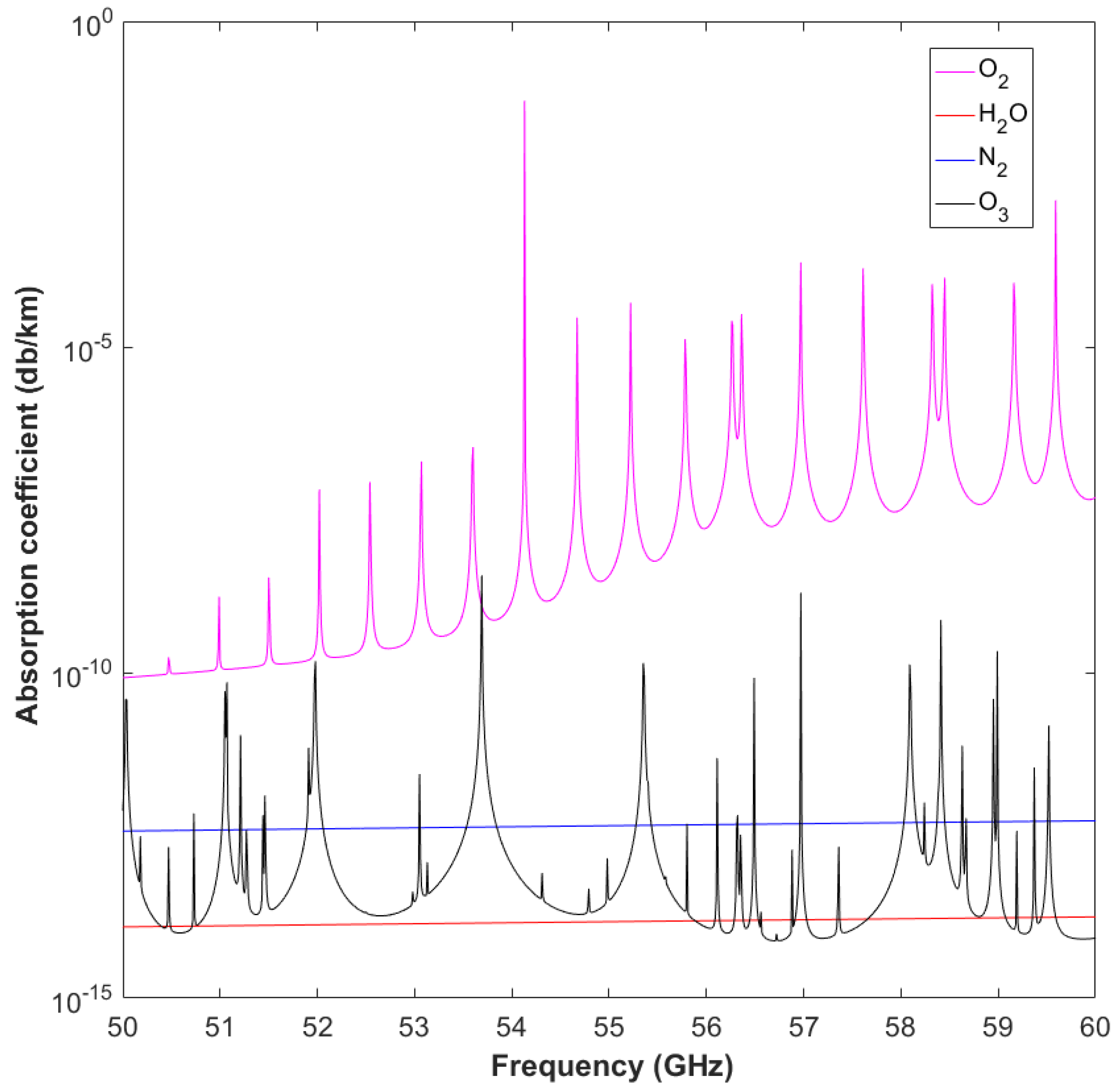
With its complex and numerous absorption lines, the 60 GHz band provides good sensitivity to temperature all along the atmospheric profile. Figure 1 illustrates the absorption coefficients calculated by ARTS for different absorbers in the 50–60 GHz frequency band, where water vapor data and oxygen data were sourced from the MPM89 model and MPM93 model, respectively. In the 50–60 GHz band, the ${\mathrm{O}}_2$ absorption is dominant, and there are several ${\mathrm{O}}_2$ absorption lines with different intensities, among which there are bi-modal absorption lines near 56 GHz and 58 GHz. In the 50–60 GHz band, ${\mathrm{H}}_2\mathrm{O}$ and ${\mathrm{N}}_2$ are continuously absorbing, and the absorption of ${\mathrm{O}}_3$ fills the whole frequency band, but it is generally weaker than that of ${\mathrm{O}}_2$.

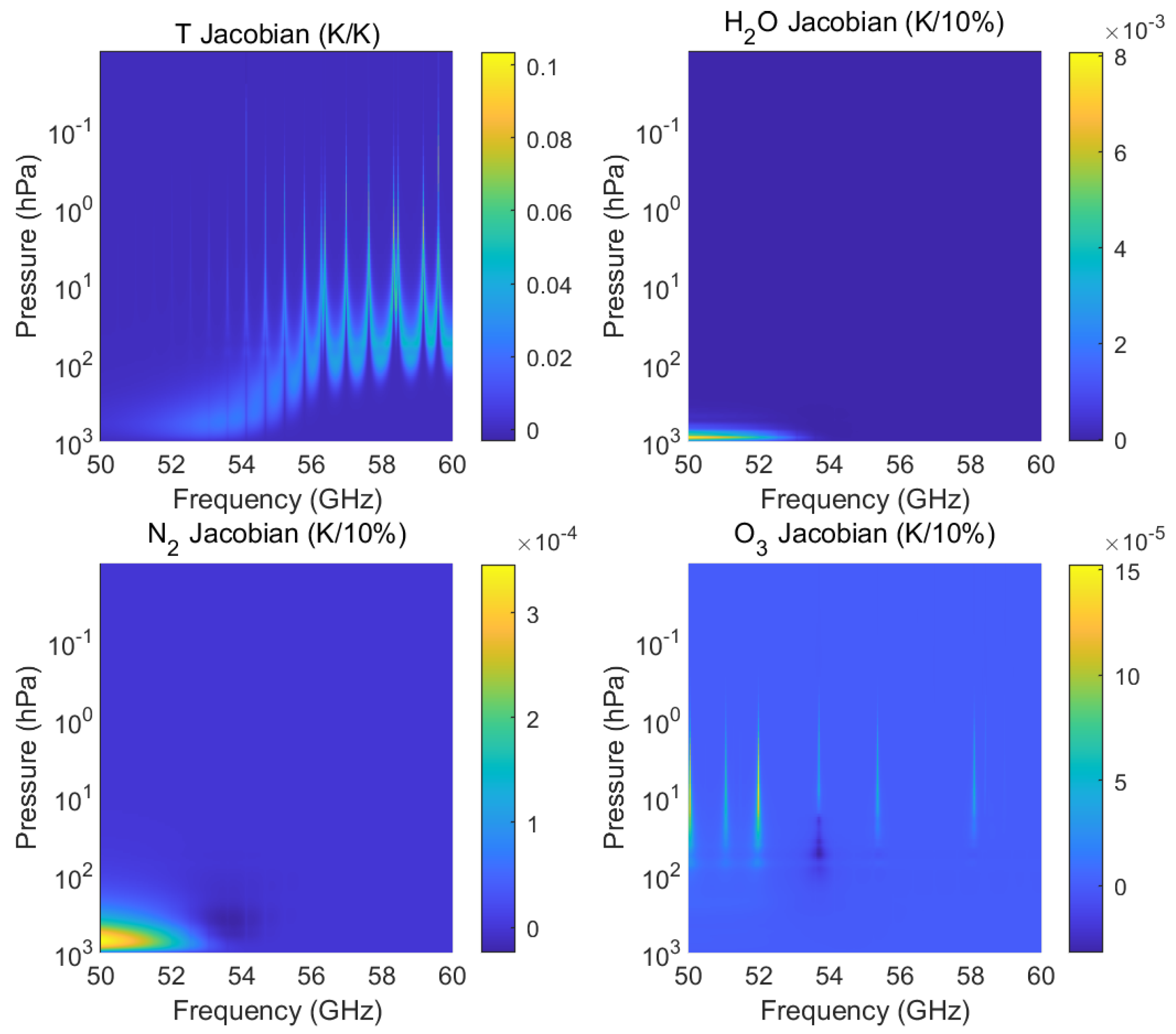
In order to show the influence of different absorbers, changes in brightness temperature were obtained by altering the perturbation values of the absorbers layer by layer, with perturbations of 10% for ${\mathrm{H}}_2\mathrm{O}$, ${\mathrm{N}}_2$, and ${\mathrm{O}}_3$ and 1 K for temperature ($\mathrm{T}$). The Jacobian matrix of $\mathrm{T}$, ${\mathrm{H}}_2\mathrm{O}$, ${\mathrm{N}}_2$, and ${\mathrm{O}}_3$ is shown in Figure 2. Figure 2 shows that based on 10 MHz, when the temperature is perturbed, the variation in brightness temperature is mainly between 0.02 K and 0.1 K. When ${\mathrm{H}}_2\mathrm{O}$, ${\mathrm{N}}_2$, and ${\mathrm{O}}_3$ are perturbed, the variation in brightness temperature is mainly between ${10}^{-5}$ K and ${10}^{-3}$ K. It can be seen that the influence of ${\mathrm{H}}_2\mathrm{O}$, ${\mathrm{N}}_2$, and ${\mathrm{O}}_3$ have very little effect on brightness temperature compared to temperature, so it can be ignored. The amplitude of the Jacobians is lower for the coarser spectral resolution. The absorption lines are thinner and sound higher in the vertical with the highest spectral resolution [23]. A higher spectral resolution captures more information within 50–60 GHz. Consequently, when the perturbations of the absorbers can be neglected based on 10 MHz, they can also be ignored based on coarser spectral resolution.

3.3. NEDT Calculation Results

The measurement error consists of the observation error and forward modeling error. The observation error refers to radiometer sensitivity, which is the noise generated in the measurement. The forward model error arises from the inaccuracies of the forward model itself and the inaccurate measurement of atmospheric state parameters. Since the method in this paper employs the same forward model for calculating radiative brightness temperature and utilizes the same atmospheric profile database, the forward model errors can be disregarded, with us only needing to consider observation errors in our calculations. Usually, when analyzing observation errors, the correlation between channels is not taken into account, and the observation error covariance matrix is assumed to be a diagonal matrix, with the diagonal elements representing the square of the sensitivity [24].

The observation errors should be specified. The NEDT can be calculated using the classical radiometric Equation [23]:

$$NEDT=(T_{receiver}+T_{antenna})/\sqrt{Bandwidth•t}$$

(8)

$$T_{receiver}=4.5\times F\left(Ghz\right)+30$$

(9)

where $T_{receiver}$ represents the equivalent noise temperature of the receiver, $T_{antenna}$ represents the antenna temperature that is approximately equal to the scene brightness temperature, $Bandwidth$ is the bandwidth of the receiver, t is the integration time, and the constants are measured in kelvin (K). An average $T_{antenna}$ of 290 K is assumed. The selected integration time (t) is 16 ms for all channels, and the constants are measured in kelvin [25]. It can be seen that the NEDT theoretically varies with changes in channel bandwidth and the equivalent noise temperature of the receiver. The NEDT can be used as the observation error covariance to calculate information entropy. The random noise generated when using NEDT as the standard deviation can also be used as the noise input for subsequent retrieval.

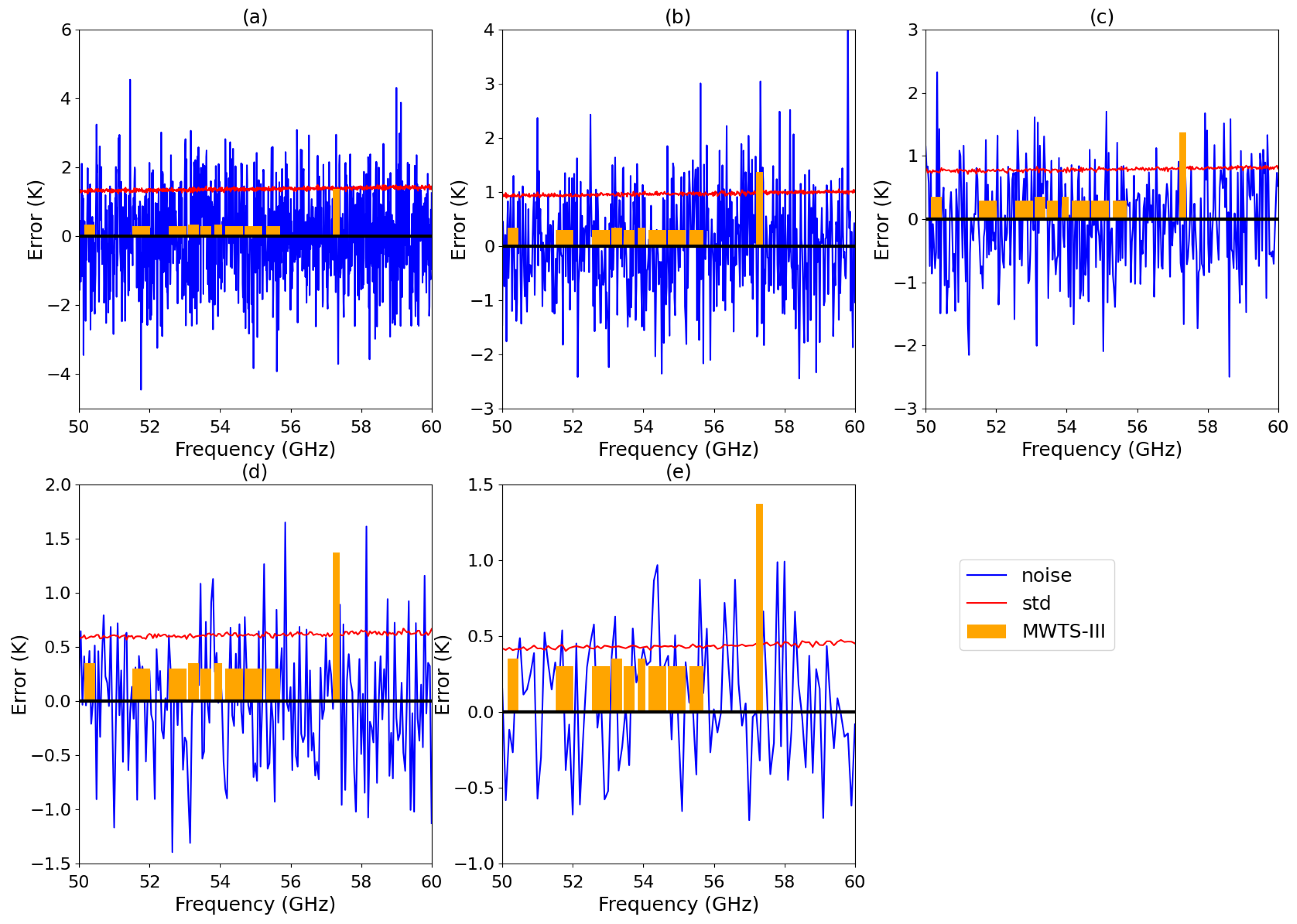
The closer the value of NEDT is to 0, the higher the observation accuracy. In this paper, the NEDT at different bandwidths is calculated according to Equations (8) and (9), and the NEDT values of MWTS-III were obtained from the website of the China National Satellite Meteorological Center (https://satellite.nsmc.org.cn/portalsite/default.aspx, accessed on 16 December 2023). The noise errors at different bandwidths are shown in Figure 3, where the blue curve indicates the random noise error and the red curve indicates the standard deviation of the measurement noise error, which approximates the NEDT; the orange bar shows the NEDT of MWTS-III. It can be seen that as the spectral resolution increases, the noise error also tends to increase. The mean values of NEDT based on 10, 20, 30, 50, and 100 MHz bandwidths are 1.37, 0.97, 0.79, 0.61, and 0.43 K, respectively. The corresponding NEDT value for the detection channel of MWTS-III set at 50–56 GHz is approximately 0.3 K, while the detection channels set at 57 GHz have a higher spectral resolution, resulting in a larger NEDT value. The NEDT of the channels in MWTS-III is generally closer to the NEDT calculated in the 100 MHz bandwidth.

3.4. Background Error

The background error covariance matrix is calculated as shown in Equation (10):

$$B=\frac{(x-\overline{x}){(x-\overline{x})}^T}{n-1}$$

(10)

where x denotes the atmospheric temperature profile, $\overline{x}$ denotes the sample mean, and n denotes the number of atmospheric profile samples.

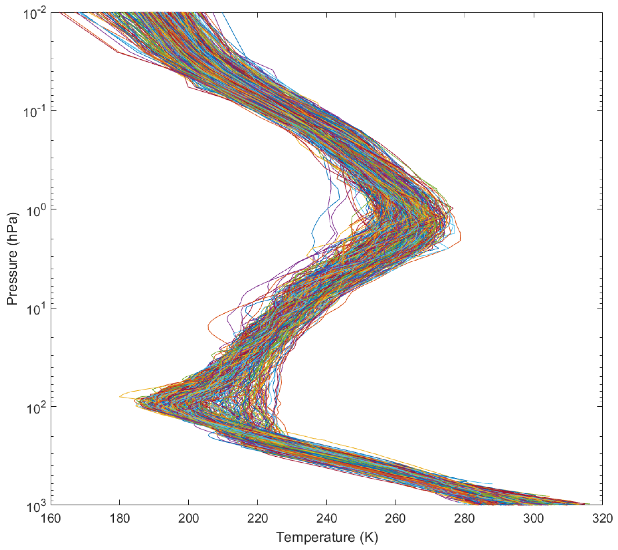
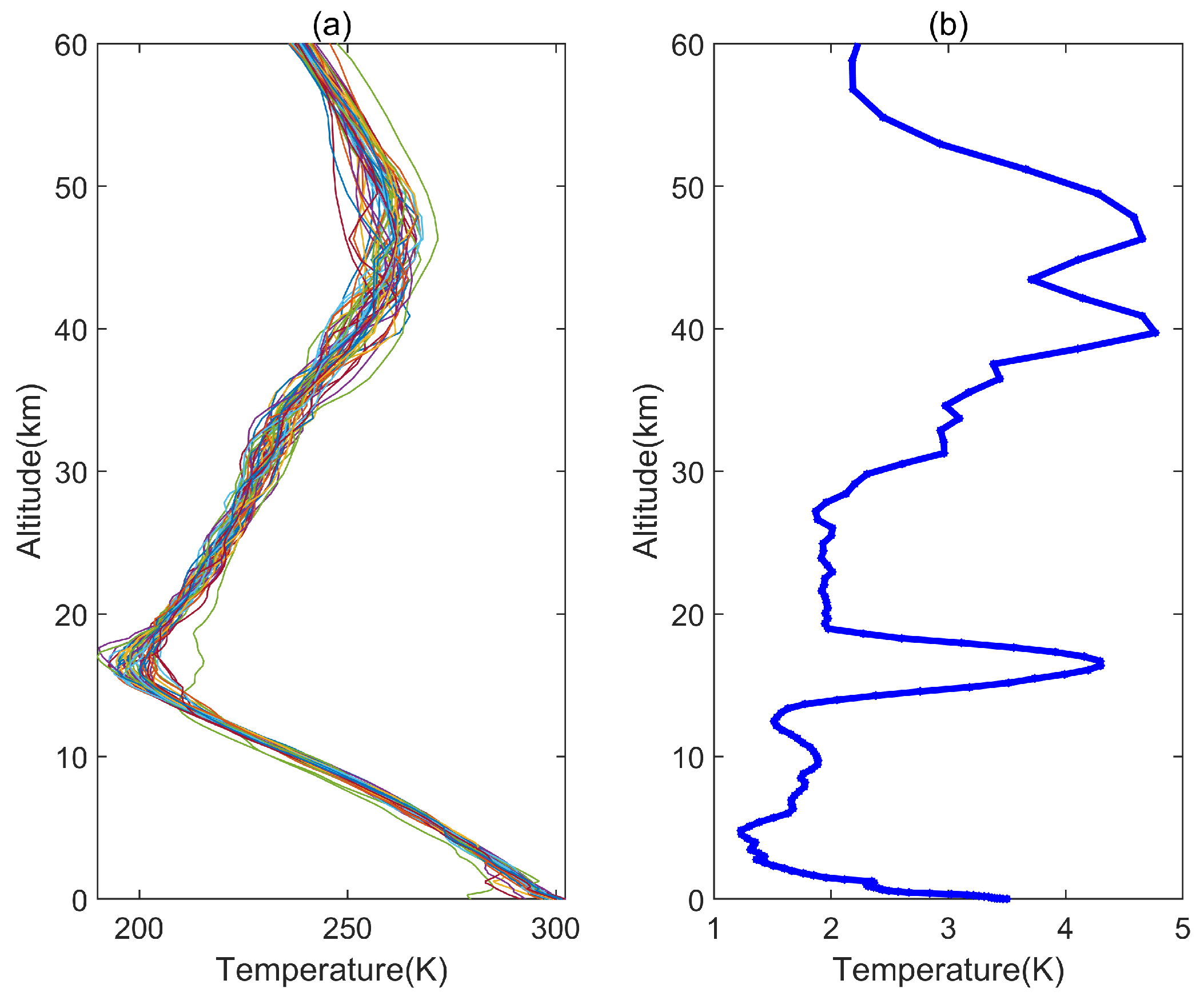
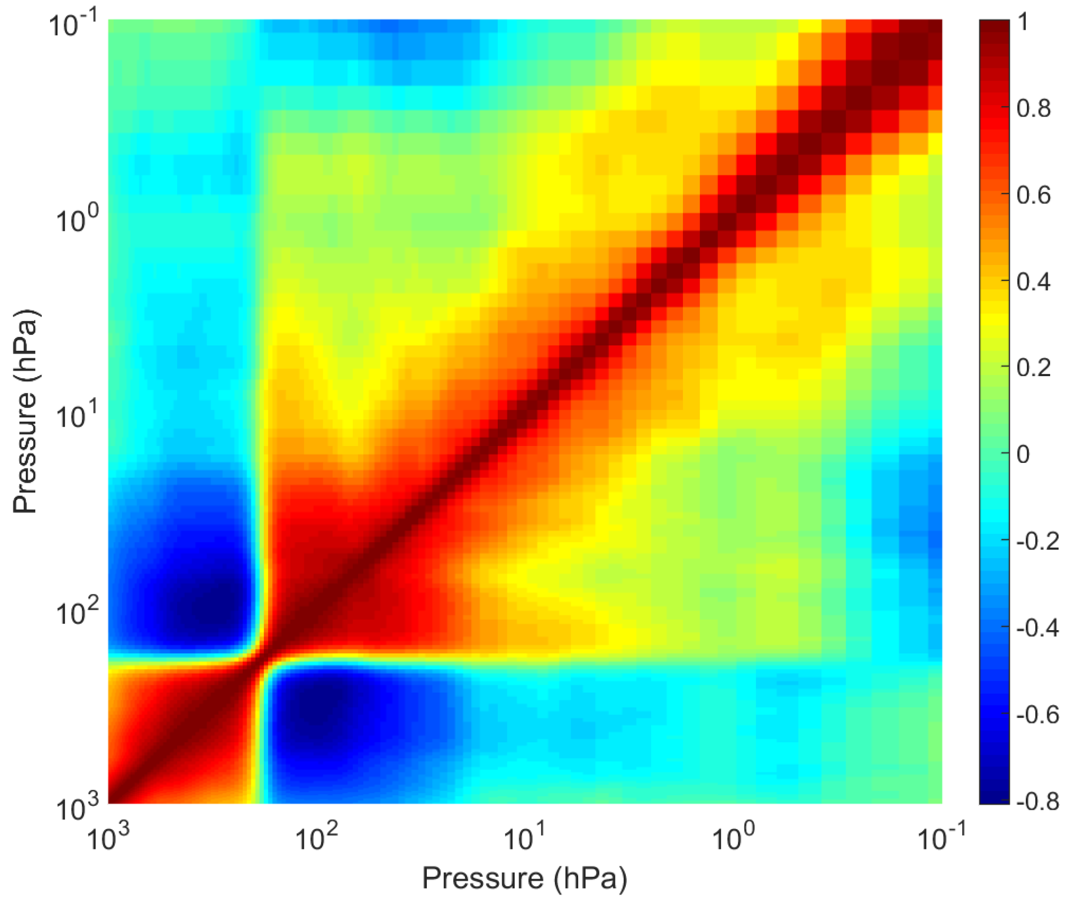
In this paper, the background error covariance is based on the statistical results of global samples, and the background error covariance matrix reflects the statistical characteristics of atmospheric temperature; this is related to the selection of temperature profiles, and the selected atmospheric profile is shown in Figure 4, where the different color lines represent different atmospheric temperature profiles. Since the background error covariance matrix represents the correlation between atmospheric temperatures at different altitudes, the background error covariance matrix can be represented by the correlation coefficient matrix, as shown in Figure 5. It can be seen that the correlation coefficient ranges from −0.8 to 1, where red indicates the region with a large correlation coefficient, which is mainly distributed near the diagonal and indicates a strong correlation between adjacent atmospheres. In the lower atmosphere, the temperature field has a strong vertical correlation, with a correlation coefficient greater than 0.6, and there is a strong negative correlation at 200 hPa.

3.5. Information Entropy Method

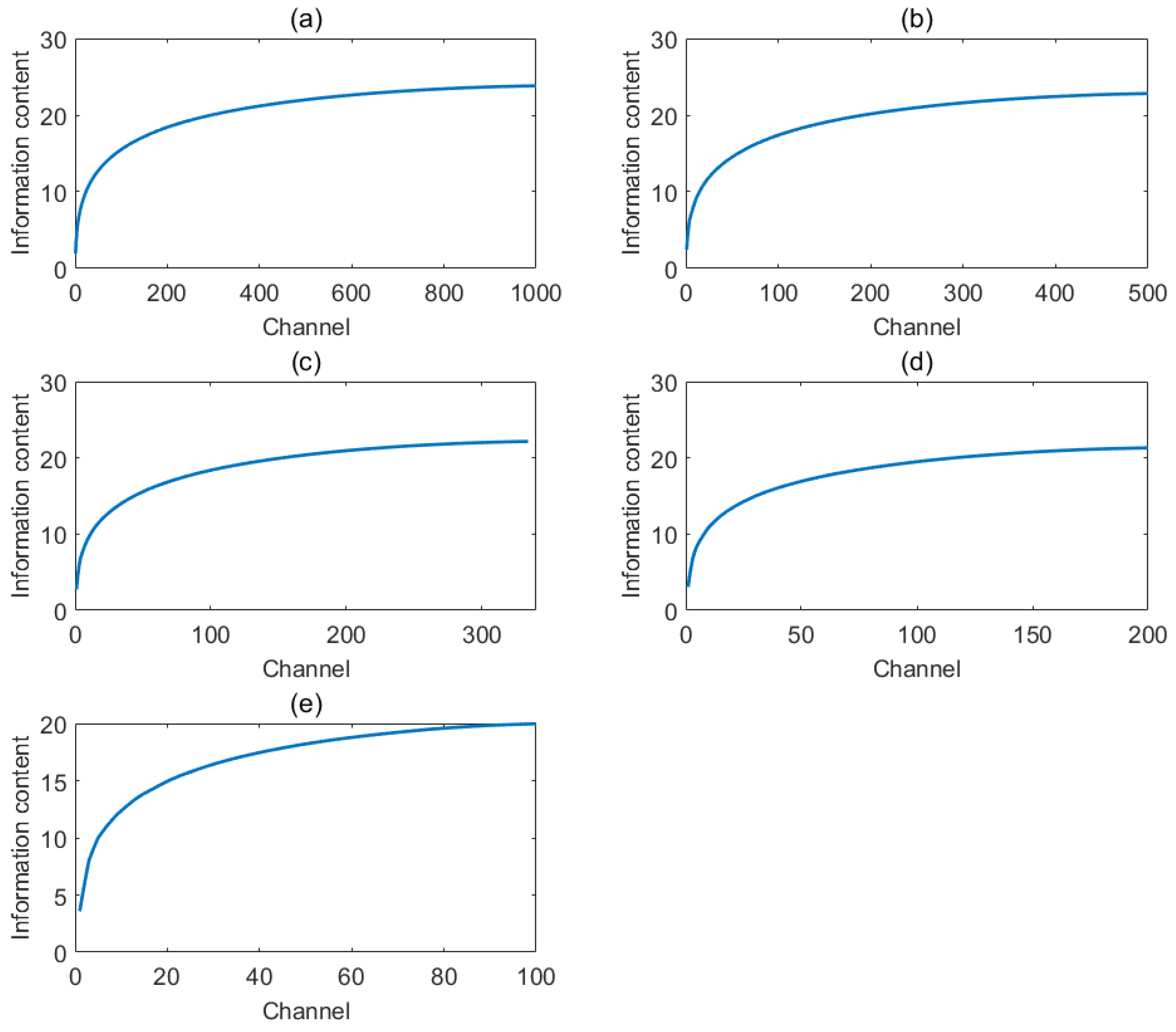
Based on different bandwidths, the information entropy method was used to select the channels. When the bandwidth was set to 10, 20, 30, 50, and 100 MHz, the total number of channels in the 50–60 GHz band was 1000, 500, 334, 200, and 100, respectively. Figure 6 shows the number of channels versus the total information content for different bandwidth conditions. It can be seen that as the channel bandwidth becomes wider, the total information content contained gradually decreases. The total information content extracted increases with the number of channels selected. When fewer channels are selected, the total information entropy increases rapidly with the increase in the number of channels, but when the number of selected channels reaches a certain level, the increasing trend of the total information entropy slows down.

This shows that a portion of the channels ranked at the top of the channel selection contains a large amount of information and that the channels ranked at the bottom have very low information content. Therefore, in the 50–60 GHz frequency band, we selected an appropriate number of channels while ensuring that most of the channel information content was included to reduce the computational scale of the atmospheric temperature profile retrieval model and improve the retrieval efficiency of the atmospheric temperature profile.

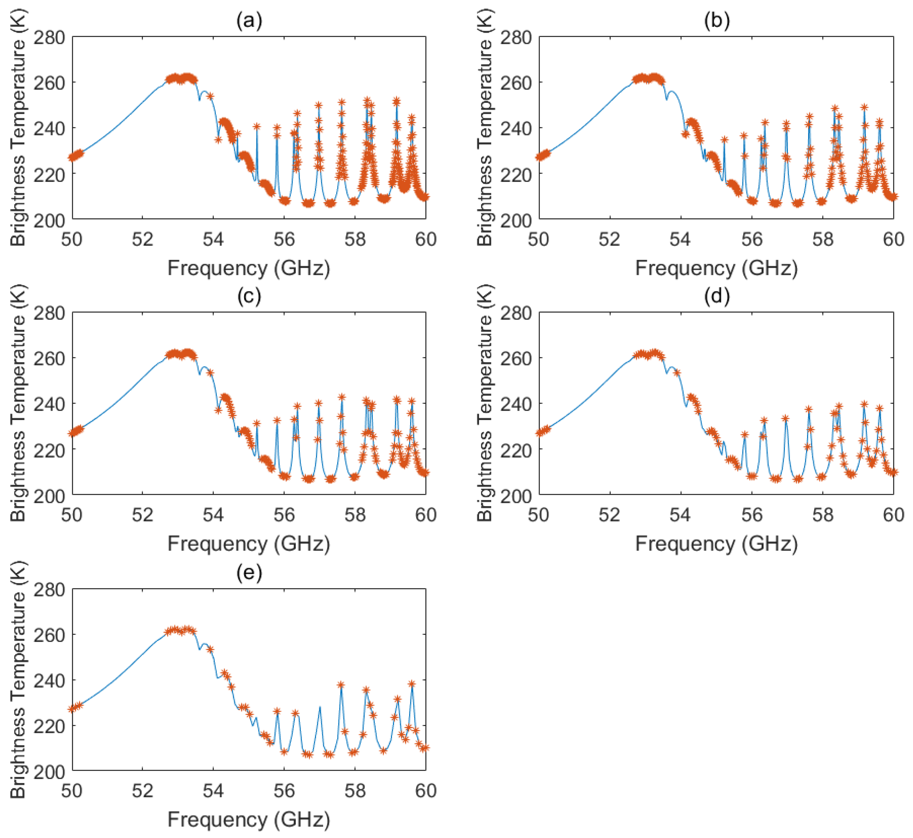
When using the information entropy method for channel selection, 90% of the total information content was taken as the criterion, at which point the selected channel contains most of the information [26]. The frequency distribution of selected channels at different bandwidths is shown in Figure 7. The blue curve in Figure 7 indicates the curve of radiation brightness temperature versus frequency, and orange symbol represents the center frequency of the selected channel. It can be seen that most of the selected channels are located at the abrupt changes in the radiation brightness temperature curve and are mainly concentrated between 53 and 60 GHz. After channel selection using the information entropy method, the number of channels at bandwidths of 10, 20, 30, 50, and 100 MHz was 435, 225, 152, 93, and 47, respectively.

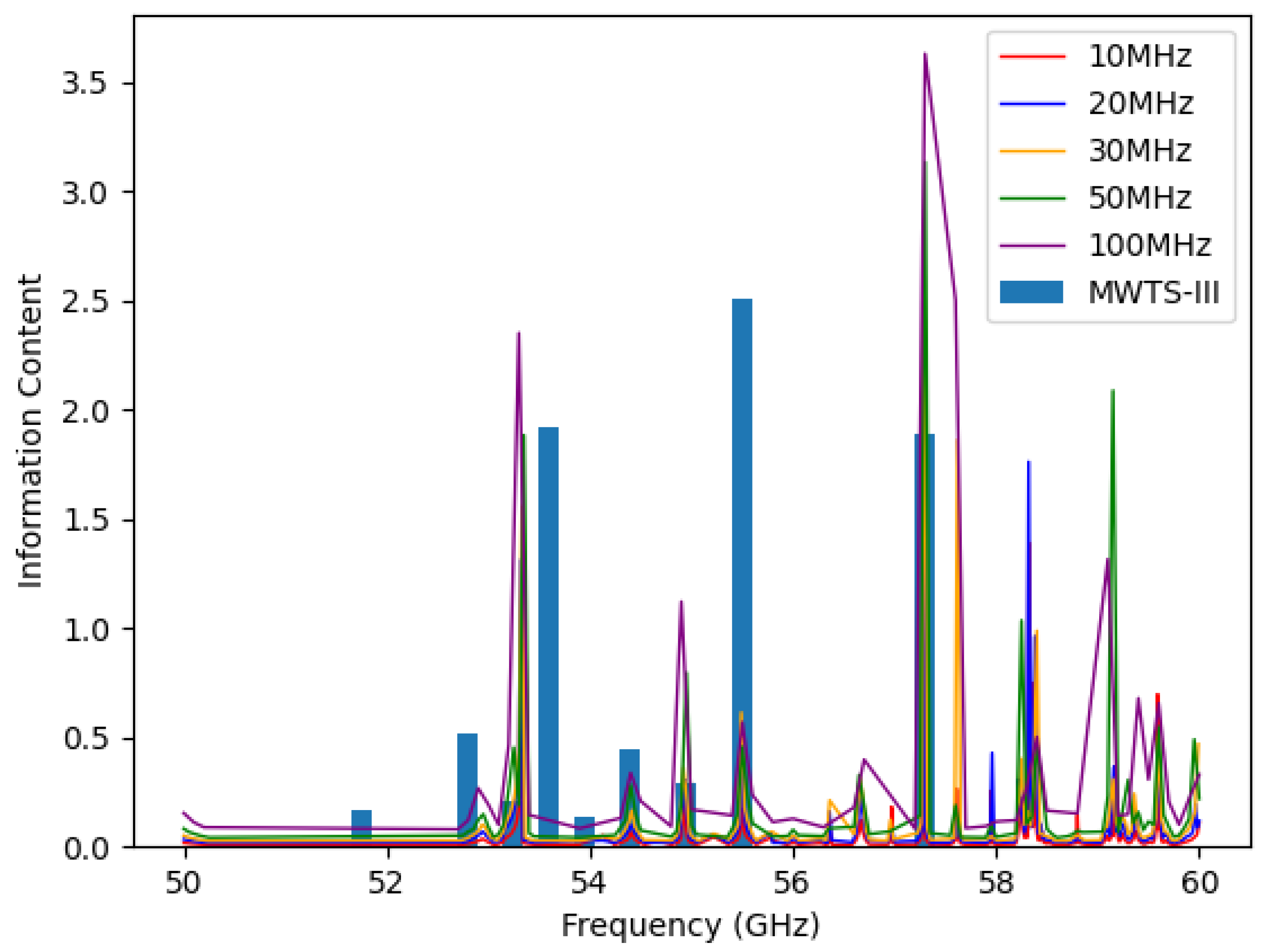
The channels were selected based on the information entropy method, and the information content of the selected channels at different bandwidths was calculated. Figure 8 shows the information content of each channel for MWTS-III and the different bandwidths. It can be seen that the channels of MWTS-III set near 57.29 GHz, 55.5 GHz, and 53 GHz contain more information. The channels with different bandwidth settings at 57 GHz, 58 GHz, 53 GHz, and 59 GHz contain more information content. The number of channels and information content at each frequency band for MWTS-III and the different bandwidths are shown in

Table 1. A comparison of the number of channels and information content at each frequency band for MWTS-III and different bandwidths.

	10 MHz	20 MHz	30 MHz	50 MHz	100 MHz	MWTS-III
50–51 GHz	24/0.29	13/0.31	9/0.32	6/0.35	3/0.35	1/0.03
51–52 GHz	0/0	0/0	0/0	0/0	0/0	1/0.17
52–53 GHz	28/0.55	14/0.54	9/0.52	5/0.48	3/0.47	1/0.51
53–54 GHz	44/3.07	22/3.09	16/3.14	11/3.22	6/3.33	3/2.26
54–55 GHz	53/1.79	28/1.75	18/1.68	10/1.86	5/1.89	2/0.74
55–56 GHz	45/1.57	25/1.63	17/1.63	10/1.31	5/1.23	1/2.51
56–57 GHz	42/1.40	21/1.38	15/1.41	9/0.99	4/0.79	0/0
57–58 GHz	42/3.86	22/3.69	13/5.20	8/3.76	5/6.39	6/1.89
58–59 GHz	61/5.26	30/4.88	22/2.82	14/2.55	6/1.32	0/0
59–60 GHz	96/4.29	50/3.89	33/3.81	20/5.28	10/4.10	0/0

. It can be seen that most of the selected channels at different bandwidths are located within 53–60 GHz, with the highest number of selected channels within 59–60 GHz; no channels were selected within 51–52 GHz, indicating that the information content contained in the channels within this band is minimal and has been eliminated. The channels within 50–51 GHz and 52–53 GHz at different bandwidths contain little information content, whereas the channels within 57–60 GHz contain a lot of information content. Specifically, the channels within 57–58 GHz at the 100 MHz bandwidth contain the highest amount of information content, reaching up to 6.39. Compared to MWTS-III, the number of selected channels at different bandwidths is greater and contains more information content.

3.6. Weighting Function

After selecting channels using the information entropy method, the weighting function was calculated for the selected channel according to Equation (11):

$$WF=\frac{\partial \tau (v,\theta ,P)}{\partial lnP}$$

(11)

where $\partial \tau (v,\theta ,P)$ represents the transmittance of the channel corresponding to wave number v, which depends on the absorption coefficient of the absorbing gas in the atmosphere. $\theta$ represents the zenith angle observed by satellites, and P represents the atmospheric pressure.

The ideal weighting function should exhibit a single peak. If the weighting function exhibits multiple peaks, the detection altitude corresponding to the channel will not be unique, making it difficult to determine from which altitude the information detected by the channel originates. Therefore, channels with multiple peaks in the weighting function should be eliminated. In order to minimize the number of detection channels, when the detection layers of channels are at the same altitude, the channel with the largest weighting function value should be selected.

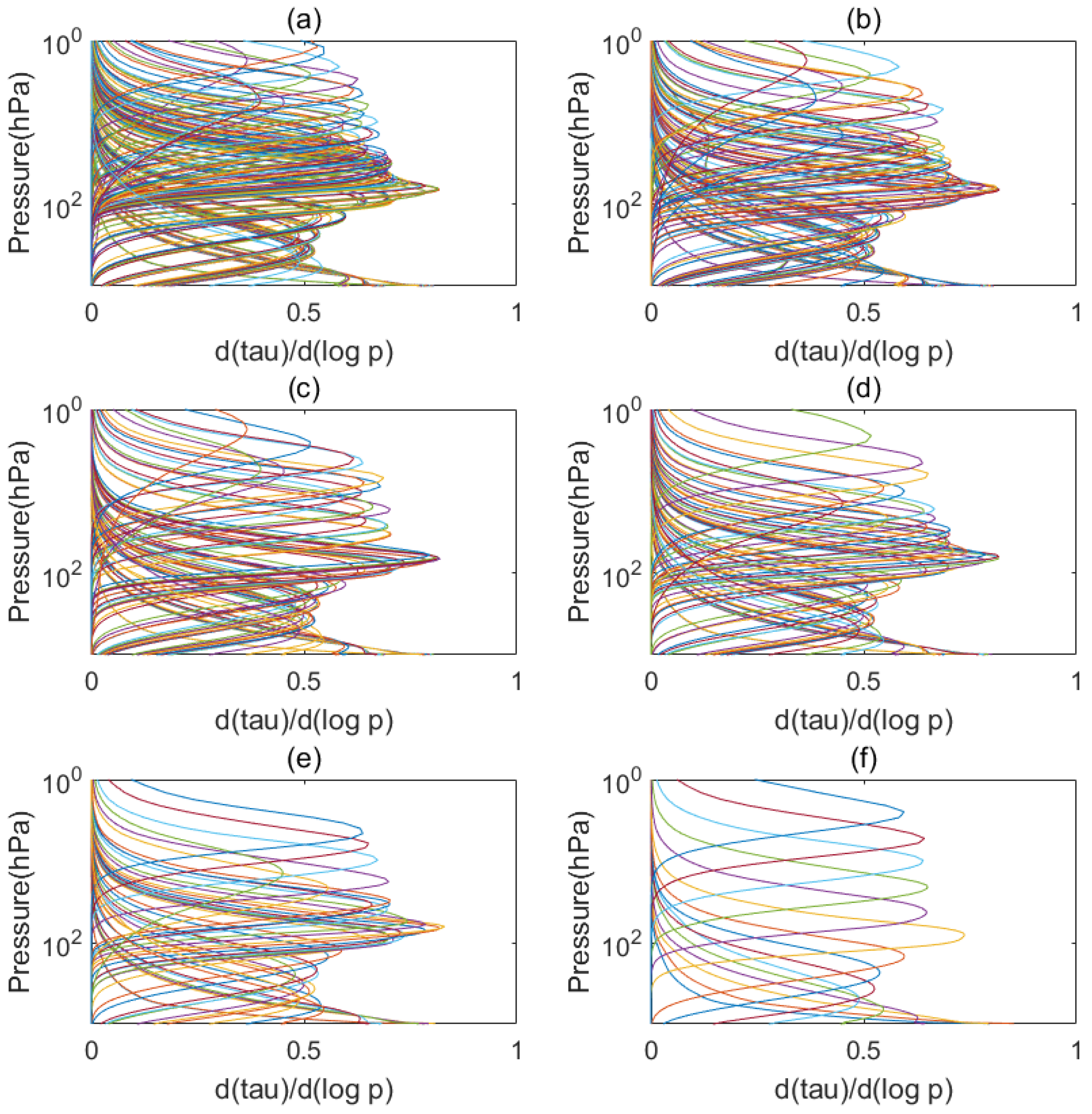
After the weighting function was used for channel selection, the weighting function for MWTS-III and for different bandwidths was calculated and is shown in Figure 9, where different color lines represent different channels. It can be seen that the selected channels at different bandwidths cover more detection layers than MWTS-III. Additionally, as the bandwidth narrows, the effective detection height increases. Each altitude retains at least one detection channel, which ensures high vertical resolution for detecting the atmosphere. After channel selection by the weighting function, the number of channels based on the 10, 20, 30, 50, and 100 MHz bandwidths is 186, 112, 86, 54, and 36, respectively.

4. Comparison of Experimental Results

In order to compare the results of the channel selections at different bandwidths, the Qpack tool and statistical retrieval method OEM were used for retrieval verification based on the selected frequencies [21]. The retrieval atmospheric profiles used in this study are shown in Figure 10, where different color lines represent different atmospheric profiles. The prior profile is set as the average of the atmospheric profile dataset. The cost function is defined as Equation (12) [27]:

$${\chi }^2={[y-F(x,b)]}^T{A}^{-1}[y-F(x,b)]+{[x-x_a]}^T{B}^{-1}[x-x_a]$$

(12)

where y is the simulated real brightness temperature, which is the sum of the simulated true profile brightness temperature and Gaussian noise, where the system sensitivity is the standard deviation, $F(x,b)$ is the ARTS model, x is the profile produced by each iteration, $x_a$ is the background profile, B is the background error covariance, and A is the observation error covariance.

The iteration stops when $\frac{X_{n+1}^2-X_n^2}{X_n^2}$ < 0.01 or the number of iterations exceeds 20. The Marquardt–Levenberg algorithm was used for the iteration process. The retrieval results were counted and compared, and the RMSE is defined as

$$RMSE=\sqrt{\frac{1}{N}\sum _{i=1}^N{(x_{true}-x_{retrieval})}^2}$$

(13)

where $x_{true}$ denotes the true profile, $x_{retrieval}$ denotes the retrieval profile, and N denotes the number of samples.

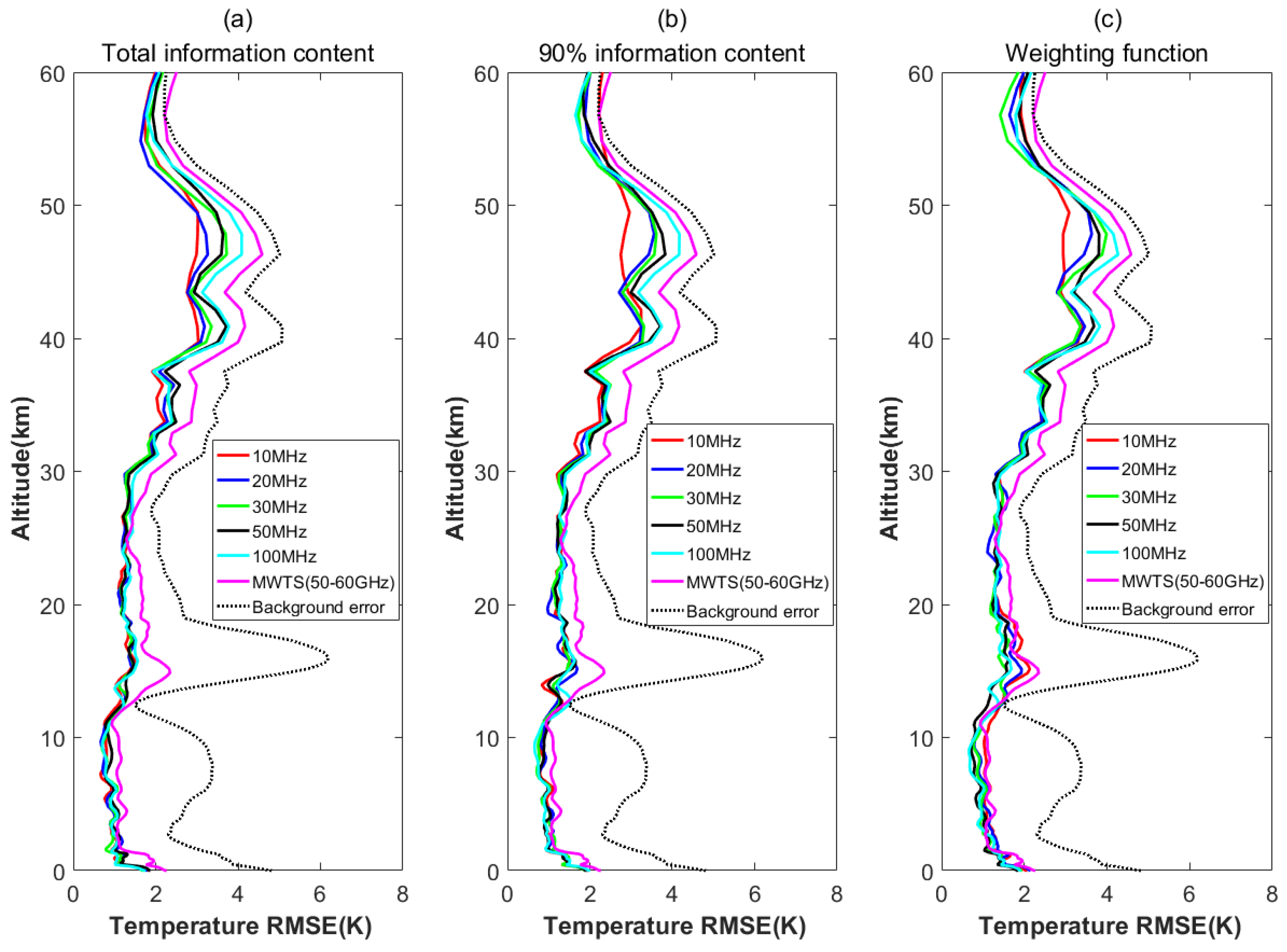
Figure 11 shows the retrieval results before and after channel selection. It can be seen that the retrieval results before and after channel selection at different bandwidths are better than those of MWTS-III, and the performance is particularly evident in the middle and upper atmosphere.

The retrieval results using total information content are shown in

Table 2. Retrieval results using total information content.

	Channel	Troposphere RMSE (K)	Stratosphere RMSE (K)	Whole Atmosphere RMSE (K)
10 MHz	1000	0.9001	1.5182	1.7428
20 MHz	500	0.9283	1.5577	1.7766
30 MHz	334	0.9298	1.6262	1.8558
50 MHz	200	0.9926	1.6904	1.9373
100 MHz	100	0.9408	1.7579	1.9762
MWTS-III	15	1.2024	2.0732	2.3531

. Additionally, the retrieval results utilizing 90% information content are summarized in

Table 3. Retrieval results utilizing 90% information content.

	Channel	Troposphere RMSE (K)	Stratosphere RMSE (K)	Whole Atmosphere RMSE (K)
10 MHz	435	1.0020	1.5318	1.8307
20 MHz	225	1.0079	1.6163	1.8667
30 MHz	152	0.9829	1.6444	1.8730
50 MHz	93	0.9994	1.6983	1.9376
100 MHz	47	0.9526	1.7694	1.9734
MWTS-III	15	1.2024	2.0732	2.3531

, and the retrieval results after weighting function selection are detailed in

Table 4. Retrieval results after weighting function selection.

	Channel	Troposphere RMSE (K)	Stratosphere RMSE (K)	Whole Atmosphere RMSE (K)
10 MHz	186	1.1922	1.6709	1.9533
20 MHz	112	1.1230	1.7078	1.9554
30 MHz	86	1.0334	1.7129	1.9162
50 MHz	54	0.9630	1.7543	1.9828
100 MHz	36	0.9944	1.7792	2.0036
MWTS-III	15	1.2024	2.0732	2.3531

. It can be seen that the retrieval results using the total information content at different bandwidths are the best in the troposphere, stratosphere, and whole atmosphere. Furthermore, these results basically abide by the rule that the higher the spectral resolution, the better the retrieval. When using information entropy for channel selection, the number of channels decreases by about 54.44%, and its RMSE increases slightly. After selecting channels using weighting functions, the number of channels was further reduced, and the channel selection method reduces the number of channels by a total of about 74.05%. It can be seen that the channel selection method eliminates too many channels in the 10 MHz bandwidth, and the increase in noise caused by its narrow bandwidth has largely offset the beneficial effects of having multiple channels, resulting in poorer retrieval performance in the troposphere. After channel selection, the performance of the 50 MHz bandwidth is the best in the troposphere, the performance of the 10 MHz bandwidth is the best in the stratosphere, and the performance of the 30 MHz bandwidth is the best in the whole atmosphere.

Overall, the retrieval results before and after channel selection all show positive effects compared to MWTS-III. Although the retrieval results after channel selection are slightly worse than those using all channels, the channel selection scheme is effective when considering the number of channels, the size of the computation, and the retrieval results comprehensively. At different altitudes, the selected channels based on different bandwidths perform differently. Therefore, when designing channels, it is advisable to consider different bandwidths for different altitudes to achieve better retrieval results.

5. Conclusions

Compared to infrared, microwaves can sound atmospheric temperature and humidity information below thin clouds. Therefore, it is important to apply hyperspectral technology to the microwave band. Considering that the detection of atmospheric temperature profiles helps to describe atmospheric evolution and monitor climate, the research in this paper sought to apply hyperspectral technology within the 50–60 GHz band. In this study, we performed channel selection based on the channel bandwidth, information entropy, and weighting function. In order to investigate the influence of channel selection at different bandwidths, we used the retrieval RMSE as the standard to measure the effectiveness of channel selection. The experimental results show that trace gases do not affect the forward modeling accuracy of the channel for the selected five bandwidths when performing spectral analysis on the 50–60 GHz frequency band. When selecting channels containing 90% of the total information content, the selected five bandwidths retained 435, 225, 152, 93, and 47 channels, respectively. The channels were further selected using the weighting function to eliminate the channels with high correlation, and the final number of channels retained for the selected five bandwidths was 186, 112, 86, 54, and 36. The experimental results show that channel selection can reduce the number of channels by about 74.05% while maintaining a large amount of information content, and the retrieval effect is significantly better than that of MWTS-III. After channel selection, the 10 MHz, 30 MHz, and 50 MHz bandwidths have the best retrieval results in the stratosphere, whole atmosphere, and troposphere, respectively. At different altitudes, the selected channels based on different bandwidths perform differently. Therefore, when designing channels, it is advisable to consider different bandwidths for different altitudes to achieve better retrieval results. Considering the number of channels, computational scale, and retrieval results comprehensively, the channel selection method is effective.

However, the atmospheric profiles used for channel selection in this paper were those under clear-sky conditions, which may not apply to other weather conditions; therefore, our subsequent work will focus on channel selection based on complex weather conditions such as clouds and rain.

References

- Ohring, G. Impact of Satellite Temperature Sounding Data on Weather Forecasts. Bull. Am. Meteorol. Soc. 1979, 60, 1142–1147. [Google Scholar] [CrossRef]
- Le Marshall, J.; Jung, J.; Derber, J.; Chahine, M.; Treadon, R.; Lord, S.J.; Goldberg, M.; Wolf, W.; Liu, H.C.; Joiner, J.; et al. Improving Global Analysis and Forecasting with AIRS. Bull. Am. Meteorol. Soc. 2006, 87, 891–895. [Google Scholar] [CrossRef]
- Le Marshall, J.; Jung, J.; Derber, J.; Treadon, R.; Lord, S.J.; Goldberg, M.; Wolf, W.; Liu, H.C.; Joiner, J.; Woollen, J.; et al. Impact of atmospheric infrared sounder observations on weather forecasts. EoS Trans. 2005, 86, 109–116. [Google Scholar] [CrossRef]
- Pougatchev, N.; August, T.; Calbet, X.; Hultberg, T.; Oduleye, O.; Bingham, G. IASI temperature and water vapor retrievals—Error assessment and validation. Atmos. Chem. Phys. 2009, 9, 6453–6458. [Google Scholar] [CrossRef]
- Mcnally, A.P.; Watts, P.D.; Smith, J.A.; Engelen, R.; Kelly, G.A.; Thépaut, J.N.; Matricardi, M. The assimilation of AIRS radiance data at ECMWF. Q. J. R. Meteorol. Soc. 2006, 132, 935–957. [Google Scholar] [CrossRef]
- Eresmaa, R.; Letertre-Danczak, J.; Lupu, C.; Bormann, N.; McNally, A.P. The assimilation of Cross-track Infrared Sounder radiances at ECMWF. Q. J. R. Meteorol. Soc. 2017, 143, 3177–3188. [Google Scholar] [CrossRef]
- Wang, P.; Li, Z.; Li, J.; Schmit, T.J. Added-value of GEO-hyperspectral Infrared Radiances for Local Severe Storm Forecasts Using the Hybrid OSSE Method. Adv. Atmos. Sci. 2021, 38, 1315–1333. [Google Scholar] [CrossRef]
- Solman, F.; Staelin, D.; Kerekes, J.; Shields, M. A microwave instrument for temperature and humidity sounding from geosynchronous orbit. In Proceedings of the IGARSS ’98. Sensing and Managing the Environment. 1998 IEEE International Geoscience and Remote Sensing. Symposium Proceedings. (Cat. No.98CH36174), Seattle, WA, USA, 6–10 July 1998; Volume 3, pp. 1704–1707. [Google Scholar] [CrossRef]
- Zou, X.; Qin, Z.; Weng, F. Impacts from assimilation of one data stream of AMSU-A and MHS radiances on quantitative precipitation forecasts. Q. J. R. Meteorol. Soc. 2017, 143, 731–743. [Google Scholar] [CrossRef]
- Zhang, P.; Hu, X.; Lu, Q.; Zhu, A.; Lin, M.; Sun, L.; Chen, L.; Xu, N. FY-3E: The First Operational Meteorological Satellite Mission in an Early Morning Orbit. Adv. Atmos. Sci. 2022, 39, 1–8. [Google Scholar] [CrossRef]
- Ali, S.; Rosenkranz, P.; Staelin, D. Atmospheric Sounding Near 118 GHz. J. Appl. Meteorol. 1980, 19, 1234–1238. [Google Scholar] [CrossRef]
- Gasiewski, A.; Barrett, J.; Bonanni, P. Aircraft-based Radiometric Imaging of Tropospheric Temperature and Precipitation Using the 118.75-GHz Oxygen Resonance. J. Appl. Meteorol. 1990, 29, 620–632. [Google Scholar] [CrossRef]
- Blackwell, W.J.; Bickmeier, L.J.; Leslie, R.V.; Pieper, M.L.; Samra, J.E.; Surussavadee, C.; Upham, C.A. Hyperspectral Microwave Atmospheric Sounding. IEEE Trans. Geosci. Remote Sens. 2011, 49, 128–142. [Google Scholar] [CrossRef]
- Rodgers, C.D. Information content and optimisation of high spectral resolution remote measurements. Adv. Space Res. 1998, 21, 361–367. [Google Scholar] [CrossRef]
- Collard, A.D. Selection of IASI channels for use in numerical weather prediction. Q. J. R. Meteorol. Soc. 2007, 133, 1977–1991. [Google Scholar] [CrossRef]
- Rabier, F.; Fourrié, N.; Chafaï, D.; Prunet, P. Channel selection methods for Infrared Atmospheric Sounding Interferometer radiances. Q. J. R. Meteorol. Soc. 2002, 128, 1011–1027. [Google Scholar] [CrossRef]
- Carminati, F. A channel selection for the assimilation of CrIS and HIRAS instruments at full spectral resolution. Q. J. R. Meteorol. Soc. 2022, 148, 1092–1112. [Google Scholar] [CrossRef]
- Fan, H.; Wang, W.; Wang, J.; Han, W. Local comprehensive channel selection scheme for infrared high-spectral sounder data and its preliminary. J. Trop. Meteorol. 2022, 38, 715–730. [Google Scholar] [CrossRef]
- Buehler, S.; Eriksson, P.; Kuhn, T.; Von Engeln, A.; Verdes, C. ARTS, the atmospheric radiative transfer simulator. J. Quant. Spectrosc. Radiat. Transf. 2005, 91, 65–93. [Google Scholar] [CrossRef]
- Eriksson, P.; Buehler, S.; Davis, C.; Emde, C.; Lemke, O. ARTS, the atmospheric radiative transfer simulator, version 2. J. Quant. Spectrosc. Radiat. Transf. 2011, 112, 1551–1558. [Google Scholar] [CrossRef]
- Eriksson, P.; Jiménez, C.; Buehler, S.A. Qpack, a general tool for instrument simulation and retrieval work. J. Quant. Spectrosc. Radiat. Transf. 2005, 91, 47–64. [Google Scholar] [CrossRef]
- Eresmaa, R.; McNally, A.P. Diverse Profile Datasets from the ECMWF 137-Level Short-Range Forecasts; NWP SAF Report No. NWPSAF-EC-TR-017; European Centre for Medium-Range Weather Forecasts: Reading, UK, 2014. [Google Scholar]
- Aires, F.; Prigent, C.; Orlandi, E.; Milz, M.; Eriksson, P.; Crewell, S.; Lin, C.; Kangas, V. Microwave hyperspectral measurements for temperature and humidity atmospheric profiling from satellite: The clear-sky case. JGR Atmos. 2015, 120, 11334–11351. [Google Scholar] [CrossRef]
- Wang, W.; Wang, Z.; Duan, Y. Performance evaluation of THz Atmospheric Limb Sounder (TALIS) of China. Atmos. Meas. Tech. 2020, 13, 13–38. [Google Scholar] [CrossRef]
- Aires, F. WorkPackage 2—Clear Sky Analysis; Tech. Rep.; ESA, ESTEC: Noordwijk, The Netherlands, 2014. [Google Scholar]
- Mahfouf, J.; Birman, C.; Aires, F.; Prigent, C.; Orlandi, E.; Milz, M. Information content on temperature and water vapour from a hyper-spectral microwave sensor. Q. J. R. Meteorol. Soc. 2015, 141, 3268–3284. [Google Scholar] [CrossRef]
- Rodgers, C.D. Inverse Methods for Atmospheric Sounding: Theory and Practice; Series on Atmospheric, Oceanic and Planetary Physics; World Scientific: Singapore, 2000; Volume 2. [Google Scholar] [CrossRef]
Figure 1.
Absorption coefficients of , , , and at the top of the atmosphere in the 50–60 GHz band.
Figure 2.
The Jacobian matrix of , , , and .
Figure 3.
The measurement noise errors and std at bandwidths of (a) 10 MHz, (b) 20 MHz, (c) 30 MHz, (d) 50 MHz, (e) 100 MHz, and MWTS-III.
Figure 4.
The distribution of atmospheric temperature profiles used to calculate background error covariance.
Figure 5.
Correlation coefficient matrix of atmospheric temperature profiles.
Figure 6.
Variation in information content with the number of channels at different bandwidths of (a) 10 MHz, (b) 20 MHz, (c) 30 MHz, (d) 50 MHz, and (e) 100 MHz.
Figure 7.
The frequency distribution of selected channels at bandwidths of (a) 10 MHz, (b) 20 MHz, (c) 30 MHz, (d) 50 MHz, and (e) 100 MHz.
Figure 8.
A comparison of the information content of each channel for MWTS-III and different bandwidths.
Figure 9.
The distribution of weighting functions after selection at bandwidths of (a) 10 MHz, (b) 20 MHz, (c) 30 MHz, (d) 50 MHz, (e) 100 MHz, and (f) MWTS-III (50–60 GHz).
Figure 10.
The distribution used for retrieval of (a) atmospheric profiles and (b) std values.
Figure 11.
The retrieval results when (a) using total information content (all channels), (b) using 90% information content, and (c) after channel selection based on weighting functions.