Unsupervised Change Detection in HR Remote Sensing Imagery Based on Local Histogram Similarity and Progressive Otsu

Abstract

Unsupervised change detection of land cover in multispectral satellite remote sensing images with a spatial resolution of 2–5 m has always been a challenging task. This paper presents a method of detecting land cover changes in high-spatial-resolution remote sensing imagery. This method has three characteristics: (1) Extended center-symmetric local binary pattern (XCS-LBP) is used to extract image features to emphasize spatial context information in initial change detection. Then, spectral information is combined to improve the accuracy of change detection. (2) The local histogram distance of XCS-LBP features is used as the change vector to improve the expression of change information. (3) A progressive Otsu method is developed for threshold segmentation of the change vector to reduce the false detection rate. Four datasets with different landscape complexities and seven state-of-the-art unsupervised change detection methods were used to test the performance of the proposed method. Quantitative results showed that the proposed method reduced the false detection rate and improved the accuracy of the detection of land cover changes. The F1 score achieved by the proposed method reached 0.8688, 0.8867, 0.7725, and 0.6634, respectively, which are higher than the highest corresponding F1 score achieved by the benchmark methods (0.8533, 0.8549, 0.6545, and 0.5895, respectively).

1. Introduction

Remote sensing (RS) change detection is one of the most active research topics in the RS community [1]. It has been widely used in natural disaster management [2], urban planning [3], artificial target detection [4,5], land use/cover mapping [6,7], and environmental protection [8,9]. High-spatial-resolution (HR) RS imagery has become a typical and essential data source for regional change detection.

RS change detection methods can generally be categorized into supervised and unsupervised [10,11]. Supervised methods usually achieve higher detection accuracy than unsupervised methods because they are trained using existing ground truth. However, it is time-consuming and labor-intensive to collect enough valid training samples. Unsupervised methods have attracted more interest [12] and have become a hot topic in current research because of their high level of automation and the absence of a requirement for training samples. Many studies are gradually improving the detection accuracy of unsupervised methods [13].

Unsupervised methods usually comprise two critical components: change vector (CV) generation and change information extraction [14]. CV is generated by comparing and analyzing bitemporal images in a specific way and deriving a value that expresses information about the magnitude of the change. The larger this value, the more likely it is a changed pixel. Typical methods of CV generation include image difference [15], ratio [16], log-ratio [17], and change vector analysis (CVA) [15]. Change information extraction is the process of extracting change information from the generated CV or other features. Typical methods include clustering [18,19], threshold segmentation [20,21,22], Bayesian [23], and conditional random field methods [24]. Among these, threshold segmentation is the most widely used, such as the representative Otsu method [20].

According to the processing unit, unsupervised methods can be categorized into pixel-based and object-based methods [25]. The former are popular because of their simplicity and ease of understanding. However, they are liable to create more specks because the calculations are based on individual pixels and ignore the spatial context information of the pixels. The latter methods use spatial context information but are heavily influenced by the segmentation method [26].

Research has shown that introducing spatial context information can significantly improve detection accuracy for both supervised and unsupervised methods [27]. Spatial context information provides texture information for land cover to supplement spectral information and improve detection accuracy [27]. It benefits HR RS imagery with high spatial heterogeneity and great uncertainty in change detection. There are many methods for capturing spatial context information in RS imagery, such as the neighborhood window [28], Markov random field (MRF) [29], Gabor wavelet transform [30], local binary pattern (LBP) [31], and hypergraph [32]. Among these, LBP has the advantage of grayscale invariance [33]. Moreover, numerous typical methods based on spatial context information have emerged, such as principal component analysis (PCA)-K-means clustering using neighborhood information [28], change detection based on morphological attribute profiles [34], the adaptive object-oriented spatial-contextual extraction algorithm (ASEA) [35], change detection based on weighted CVA and improved MRF (WCIM) [36], and the deep learning model-based methods deep slow feature analysis (DSFA) [37], deep CVA (DCVA) [38], and deep Siamese kernel PCA convolutional mapping network (KPCA-MNet) [39].

However, the characteristics of HR RS imagery itself lead to two issues that require further consideration in unsupervised pixel-based change detection in HR RS imagery: (1) The limitation of the spectral domain leads to uncertainty in the spectral reflectance of the HR RS imagery itself and a lack of reliability in the differences between bitemporal HR RS images, which affects the extraction of spatial context information based on specific grayscale values. (2) The segmentation methods used for change thresholds need further refinement to improve their applicability in HR RS imagery.

A new change detection method for HR RS imagery is proposed to solve these issues. This method combines spatial context information and spectral information to improve detection accuracy and replaces single threshold segmentation with multiple and progressive threshold segmentation to reduce the false detection rate. One difference from existing methods is that our method extracts the initial change information using spatial context information only, and this process includes:

(1) introducing a variant of LBP with noise resistance and a small data scale to extract spatial context information as the initial image features to avoid extracting spatial information based on the original and specific grayscale values;

(2) generating CV based on the differences in the histograms of appropriate local ranges in the initial image features;

(3) proposing a new progressive Otsu method (POTSU) applicable to HR RS image change detection to extract change information from the generated CV.

The second difference is that region growth of the spectral CV is performed based on the spatial context information represented by the initial change information to obtain the final detection result.

Four sets of HR RS images with different spatial resolutions and landscape complexities were used to validate the proposed method, including a set of WorldView-2 images with a spatial resolution of 1.8 m, a set of SuperView-1 images with a spatial resolution of 2.0 m, and two sets of TripleSat-2 images with a spatial resolution of 3.2 m. Moreover, seven state-of-the-art unsupervised methods were used to compare the performance of the proposed method. These comprised the traditional CVA combing Otsu threshold segmentation method (TCO) [20,40], three unsupervised change detection methods based on spatial context information (PCA-K-means, ASEA, and WCIM), and three unsupervised deep-learning-based methods (DSFA, DCVA, and KPCA-MNet).

The rest of this paper is organized as follows: Section 2 introduces the method and the process. Section 3 describes experimental results and compares the detection performance of the different methods. Section 4 further discusses and analyzes the proposed method. Section 5 presents the conclusion.

2. Methodology

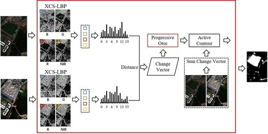
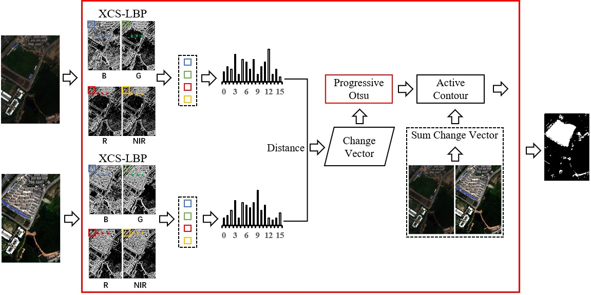
The proposed method is termed change detection based on local histogram similarity and progressive Otsu method (LHSP). It consists of three steps (Figure 1): (A) a CV is generated based on local histogram differences of the extended center-symmetric local binary pattern (XCS-LBP) [41] features; (B) the proposed POTSU segmentation achieves an initial detection result; and (C) the final change detection image (CDI) is obtained by combining the region growth of the spectral CV.

In Figure 1, T1 and T2 are bitemporal HR RS images, which include four bands, namely, blue (B), green (G), red (R), and near-infrared (NIR), respectively.

2.1. CV Generation by Local XCS-LBP Histogram Similarity

CV generation is a critical step in unsupervised change detection and directly affects the detection results. Much research has combined spatial context information to generate CVs. Still, this problem remains: spatial context information is directly extracted based on the original and specific grayscale values in many methods, such as mean values, extreme values, and key point values, which rely on the accuracy of the grayscale values. The limitation of the spectral domain in HR RS imagery may result in differences in the spectral reflectance of the same ground target in images captured at different times. In addition, there is also the phenomenon of “different spectrums for the same object and the same spectrum for different objects” in one image. This spectral error affects the reliability of spatial context information. Among algorithms used to extract spatial context information, LBP is regarded as one of the best-performing texture descriptors [42]. LBP represents spatial context information by comparing pixel grayscale values within a defined neighborhood, avoiding the effect of uncertainty in specific pixel grayscale values to some extent and having the advantage of being insensitive to changes in illumination. However, LBP is sensitive to image noise [43] and produces more complex feature sets (i.e., the histograms are too large) [44]. To tackle this problem, a variant of LBP, namely, XCS-LBP [41], was proposed. A comparison showed [41] that XCS-LBP has more advantages regarding insensitivity to noise, variations in illumination, and histogram size.

XCS-LBP comprises a binary code generated by comparing the grayscale value of the central pixel with that of a specified neighboring pixel. However, the differences in XCS-LBP values between bitemporal images cannot be used directly as the change magnitude, and the histogram distance is therefore used. To the best of our knowledge, XCS-LBP is being used for HR RS imagery change detection for the first time.

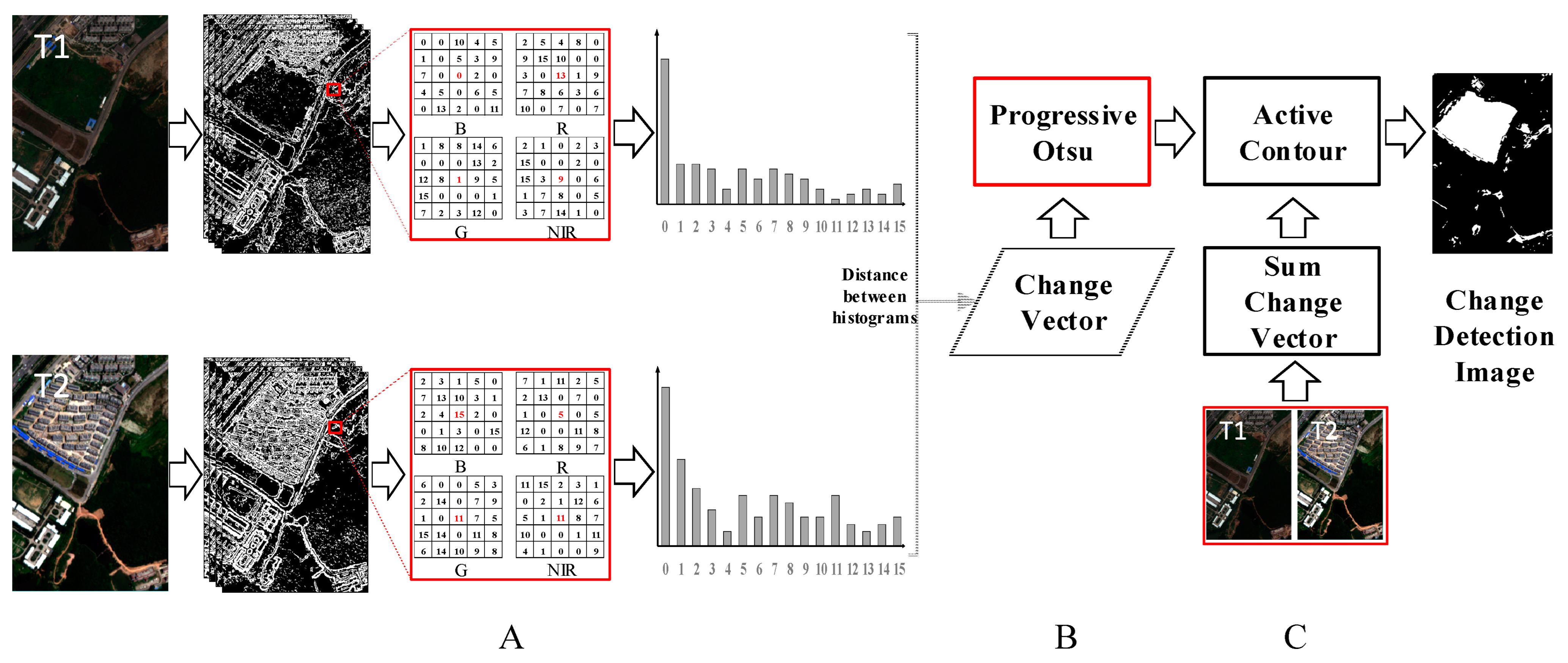
The steps to generate CV using the histogram distance of XCS-LBP are as follows:

Firstly, XCS-LBP with a neighborhood block of 3 × 3 pixels is used to extract spatial context information for each band in bitemporal images to obtain the initial image features.

Secondly, a local block is selected to construct an XCS-LBP histogram. The block’s radius should be somewhat larger than the co-registration error; otherwise, the effects of this error are relatively significant. However, it should not be too large; otherwise, the distinguishability of the central pixel will be reduced. The histogram is constructed in a block with a radius of 2 pixels (i.e., a 5 × 5-pixel neighborhood block) in our study because the average registration error can be controlled to within 1 pixel.

Thirdly, the difference in histograms for the same spatial location between the bitemporal images is calculated to generate the CV.

Histogram differences were calculated using the Euclidean distance (1) and the chi-squared distance (2) [45] to compare the effects of the histogram distance metrics:

$$\mathrm{E}\_\mathrm{d}\mathrm{i}\mathrm{s}=\sqrt{{\sum }_{h=0}^H{({\rho }_h^1-{\rho }_h^2)}^2},$$

(1)

$$\mathrm{C}\_\mathrm{d}\mathrm{i}\mathrm{s}=\sum _{h=0}^H{(({\rho }_h^1-{\rho }_h^2)}^2/({\rho }_h^1+{\rho }_h^2)),$$

(2)

where ${\rho }_h^1$ and ${\rho }_h^2$ represent the respective values in the hth column of the two histograms, the value of H is 15 (i.e., bins is 16) in XCS-LBP (all histograms have the same minimum value (0) and maximum value (15)). This way, all pixels are processed to generate one CV for change detection.

Taking bitemporal HR RS images with four bands as an example, each temporal image generates four XCS-LBP image features. Then, the values of the four XCS-LBP image features within a 5 × 5 local block (i.e., 5 × 5 × 4 feature values) are counted to construct a histogram. Finally, the differences in the histograms, pixel by pixel, between the two temporal images are calculated to generate a CV.

2.2. Generation of Initial Change Detection Image by POTSU Segmentation

The Otsu method is commonly used in change detection for the segmentation of CVs [46] and can rapidly obtain a reasonable threshold for bimodal histograms [47,48]. However, the effectiveness of segmentation by the Otsu method is not obvious when a histogram does not exhibit a clear bimodal distribution [49]. Therefore, the Otsu method is not always suitable for HR RS imagery segmentation.

This paper proposes the POTSU segmentation method to replace single Otsu segmentation. POTSU is a multiple and progressive Otsu segmentation method with a mask, whereby the segmentation results are continuously refined. The segmentation process of POTSU can be divided into two parts: progression and decision.

Progression: (1) CV is segmented by the Otsu method, and the segmentation result is obtained with changed and unchanged classes. (2) The segmentation result is used to replace the corresponding region in the merged result of the last progression (the merged result in the first progression is the segmentation result itself) in a masked manner to obtain the merged result of this progression. (3) Calculate the average interclass distance $dj$ and the average intraclass distance $di$ for the two classes in the segmentation result of this progression. For the first segmentation, $ndj=dj$ and $ndi=di$; otherwise, $ndj=dj/‖dj‖$ and $ndi=di/‖di‖$. If $ndi\ge ndj$, the changed class is extracted as a new CV in a masked manner for the next progression. If $ndi<ndj$, the unchanged class is extracted as a new CV in a masked manner for the next progression. It should be noted that distances are calculated at POTSU using Euclidean distances. (4) Steps 1–3 serve as one progression, and multiple progressions are implemented until the termination condition is reached. Here, the termination condition is set to a minimum change area (Vmin) of 500 pixels.

Decision: (1) Calculate the norm of the average intraclass distance ($nadi$) and the average interclass distance ($nadj$) for the merged results in each progression. (2) The merged result corresponding to the maximum value of $nadj-nadi$ is taken as the final result.

The pseudocode of POTSU is shown in Algorithm 1. $SR$ and $MR$ denote segmentation results and merged results, respectively. $\eta$ is the number of progressions. $w_c$ and $w_u$ represent the changed and unchanged classes, respectively.

Algorithm 1. Pseudocode of POTSU

Input: CV from Section 2.1;

Step 1: Progression    While true    $\eta =1$.     $\mathrm{C}\mathrm{V}\stackrel{Otsu}{\to }SR\left\{w_c,w_u\right\}$.     When $\eta =1$, $MR\left\{w_c,w_u\right\}=SR\left\{w_c,w_u\right\}$; otherwise, $SR\left\{w_c,w_u\right\}\stackrel{Mask}{\to }MR\left\{w_c,w_u\right\}$.     $SR\left\{w_c,w_u\right\}\stackrel{Calculate}{\to }dj,di$; When $\eta =1$,$ndj=dj$, $ndi=di$; otherwise, $ndj=dj/‖dj‖$, $ndi=di/‖di‖$.     When $ndi\ge ndj$, $\mathrm{C}\mathrm{V}=SR\left\{w_c\right\}$; otherwise, $\mathrm{C}\mathrm{V}=SR\left\{w_u\right\}$.     $\eta =\eta +1$.     Break when:     Vmin < 500 pixels.    loop Step 2: Decision     ${MR\left\{w_c,w_u\right\}}_{\eta }\stackrel{Calculate}{\to }{(nadj,nadi)}_{\eta },\eta =\mathrm{1,2},3\cdots$     ${MR\left\{w_c,w_u\right\}}_{\eta }$ is CDI when ${(nadj-nadi)}_{\eta }$ is max.

Output: CDI;

Given that the number of changed pixels is typically significantly smaller than the number of unchanged pixels in practical change detection, POTSU utilizes $ndj$ and $ndi$ to determine which objects will be segmented in the subsequent progression, as follows:

(1) When $ndi$ is greater than or equal to $ndj$, the distance between the two classes is small, and the intraclass distance is large, indicating that the two classes are poorly segmented. There are some unchanged pixels in the changed class, which increases the intraclass distance and decreases the interclass distance between the two classes, so we continue to segment the changed pixels.

(2) When $ndi$ is smaller than $ndj$, the number of changed pixels may be considered small and centrally distributed, and they are usually obvious changed pixels. However, some changed pixels with insignificant data features may be confused with unchanged pixels, so the segmentation of unchanged pixels is continued.

In summary, the former is concerned with reducing the false detection rate, while the latter is concerned with reducing the missed detection rate. Progressive segmentation is continued until the termination condition is reached.

The selection of the merged result follows the principle that a smaller intraclass distance and a larger interclass distance are better for classification. Moreover, the number of pixels to be segmented in each progression is significantly reduced compared to the previous progression because of masked segmentation, thus ensuring the timeliness of POTSU. POTSU is validated in the discussion validity of POTSU segmentation.

2.3. Generation of Final Change Detection Image

The spectral information and spatial context information from the original bitemporal images are combined in this step. The CDI from Section 2.2 is used as the seed (representing spatial context information), and the sum of the change magnitudes (representing spectral information) is segmented by a region growth method to obtain the final CDI.

The sum of the change magnitudes is represented by the sum change vector (SCV) in (3). The region growth method uses the active contour model [50,51]. All calculations are based on MATLAB R2020b with the default parameters as follows:

$${SCV}_{\left(ij\right)}=\sqrt{{\sum }_l^L{(T_{ij,l}^1-T_{ij,l}^2)}^2},$$

(3)

where 1 ≤ i ≤ m and 1 ≤ j ≤ n. Here, m and n represent the numbers of rows and columns of the bitemporal images, respectively, and $T_{ij,l}^1$ and $T_{ij,l}^2$ denote the grayscale values of (i, j) in band l for the respective bitemporal images.

The pseudocode of LHSP is shown in Algorithm 2.

Algorithm 2. Pseudocode of LHSP

Input: T1 and T2;

Step 1: Set parameters    Block size in XCS-LBP (BS1) = 3 × 3; block size for histogram construction (BS2) = 5 × 5.

Step 2: CV generation    $\mathrm{T}1\stackrel{XCS-LBP}{\to }{LBP}^{T1}$; $\mathrm{T}2\stackrel{XCS-LBP}{\to }{LBP}^{T2}$.    ${LBP}_{\left(ij\right)}^{T1}\stackrel{BS1,BS2,L}{\to }{LOCAL}_{\left(ij\right)}^{T1}$;${LBP}_{\left(ij\right)}^{T2}\stackrel{BS1,BS2,L}{\to }{LOCAL}_{\left(ij\right)}^{T2}$    Histograms ${Hist}_{\left(ij\right)}^{T1}$ and ${Hist}_{\left(ij\right)}^{T2}$ are constructed for ${LOCAL}_{\left(ij\right)}^{T1}$ and ${LOCAL}_{\left(ij\right)}^{T2}$.    $\mathrm{D}\mathrm{i}\mathrm{s}\mathrm{t}\mathrm{a}\mathrm{n}\mathrm{c}\mathrm{e}({Hist}_{\left(ij\right)}^{T1},{Hist}_{\left(ij\right)}^{T2})$ is calculated, from which a CV is generated by traversing each pixel. Step 3: POTSU segmentation    $\mathrm{C}\mathrm{V} \stackrel{POTSU}{\to }$ initial CDI. Step 4: Combined spectral-spatial segmentation    The SCV is obtained by (3).    The initial CDI is used as the seed, and the SCV is segmented using the active contour model to obtain the final CDI.

Output: Final CDI;

3. Experiments

3.1. Data Description

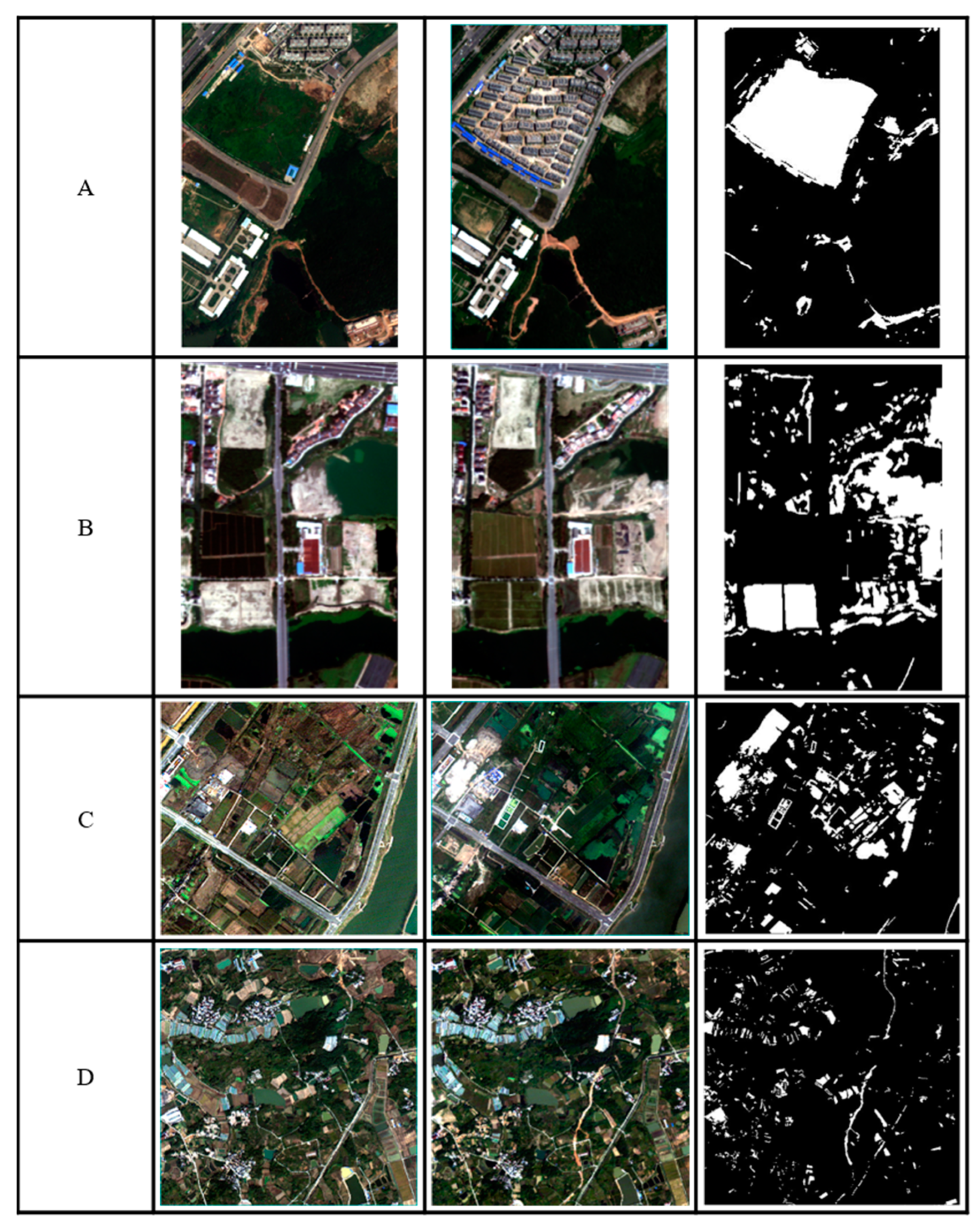
Four datasets representing multispectral RS images with differences in detection difficulty were selected to validate the proposed method (Figure 2). These were named A, B, C, and D, respectively. Dataset B was obtained from a region of Suzhou City, China, and the other datasets were obtained from Nanjing City, China. All datasets included four bands: B, G, R, and NIR. The detection difficulty in datasets C and D is significantly higher than in datasets A and B.

Dataset A comprises WorldView-2 satellite images with a spatial resolution of 1.8 m. The bitemporal images were captured in September 2013 and July 2015, respectively, and have an image size of 450 × 300 pixels. The salient change event affecting the dataset is a change from vegetation cover to building cover with a significant increase in building area, which was used to verify the effectiveness of the proposed method for change detection in general urban construction land.

Dataset B comprises SuperView-1 satellite images with a spatial resolution of 2.0 m. The bitemporal images were captured in August 2020 and October 2021, respectively, and have an image size of 450 × 300 pixels. The prominent change events are crop changes, changes in bare land and vegetation, and some building changes. This dataset was used to verify the effectiveness of the proposed method for detecting general changes.

Datasets C and D comprise TripleSat-2 satellite images with a spatial resolution of 3.2 m.

The bitemporal images in dataset C were captured in November 2016 and July 2017, respectively, and have an image size of 400 × 440 pixels. The changes highlighted in this dataset are changes in crops in agricultural areas and turnover of land type in aquaculture waters, which are greatly influenced by the season and contain a large amount of pseudo-change information. These were used to verify the effectiveness of the proposed method in removing pseudo-change information.

The bitemporal images in dataset D were captured in November 2017 and October 2018, respectively, and have an image size of 600 × 600 pixels. Numerous changes affected the dataset, such as changes in agricultural areas, residential villages, and road networks, which are more challenging to detect. This dataset was used to further validate the effectiveness of the method proposed in this paper.

The preprocessing of images included image co-registration and radiation normalization [52]. Image co-registration was performed using the Sentinel-2 images tool [53] (http://step.esa.int/main/download/snap-download/ (accessed on 1 September 2021)) with an average registration error of 0.8 pixels. The relative radiation normalization method was obtained from the literature [54].

The reference data were obtained by visual interpretation and a field survey (Figure 2).

3.2. Methods Used for Comparison and Accuracy Evaluation

3.2.1. Methods Used for Comparison

Seven change detection methods, namely, TCO [20,40], PCA-K-means [28], ASEA [35], WCIM [36], DSFA [37], DCVA [38], and KPCA-MNet [39], were used to compare their performance with that of the proposed method. Among these, the TCO was used to compare the effectiveness of the proposed method with that of the traditional threshold segmentation method. PCA-K-means, ASEA, and WCIM are methods based on spatial context information. Whereas PCA-K-means is a classical method using spatial context information and is often used for benchmark comparisons [55], ASEA and WCIM are recently proposed methods using neighborhood information. DSFA, DCVA, and KPCA-MNet are unsupervised deep-learning-based methods.

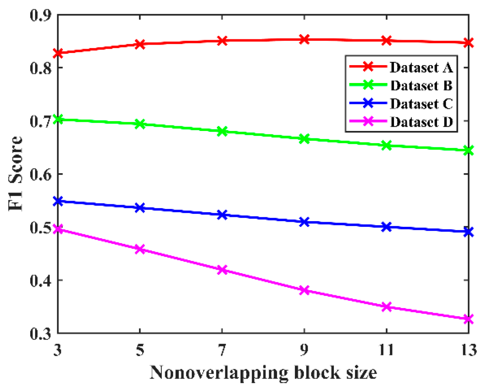
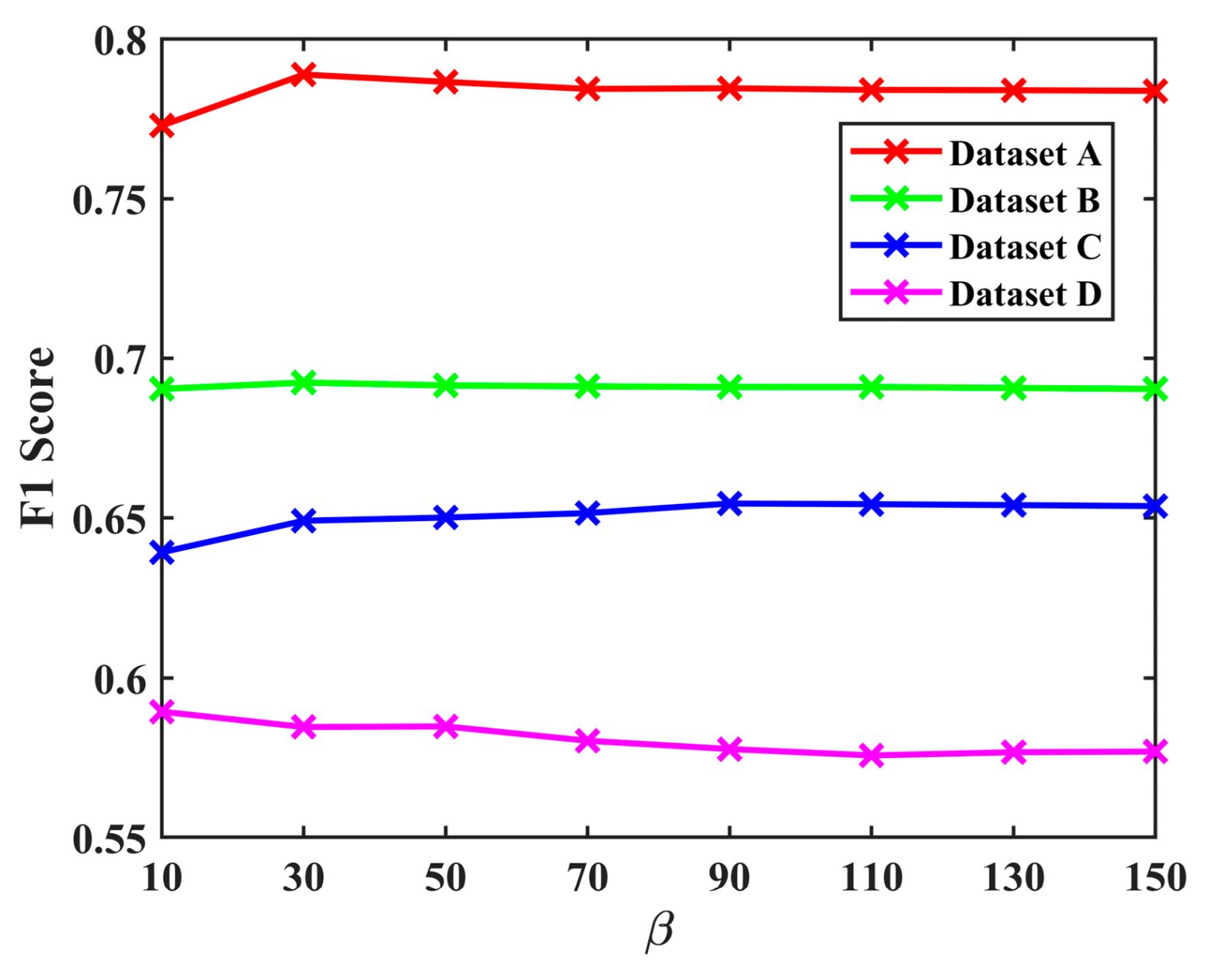
For a fair comparison, the value of nonoverlapping block size in PCA-K-means and the constant $\beta$ in WCIM were determined by our tuning (Figure 3 and Figure 4) to exhibit the optimal detection accuracy on each dataset. The parameters for other methods were kept consistent with the original papers or publicly available codes.

DSFA, DCVA, and KPCA-MNet were implemented in Python 3.10 on a computer with an Intel (R) Core (TM) i5-10300H CPU @ 2.50 GHz, 16.0 GB of RAM, and an NVIDIA GeForce GTX 1650 graphics card. The other methods were executed in MATLAB R2020b on a computer with a 3.70 GHz Intel Core i9-10900K CPU, 16.0 GB RAM, and an NVIDIA GeForce RTX 2070 graphics card.

3.2.2. Methods Used for Accuracy Evaluation

Four metrics, namely, false alarm (FA), missed alarm (MA), overall accuracy (OA), and F1 score (F1), were used to quantitatively evaluate the accuracy of change detection. Of these, FA represents the false detection rate, MA represents the missed detection rate, OA is the overall accuracy, and F1 is an evaluation indicator that integrates the precision and recall rate, as shown in (4)–(7):

$$FA=FP/(TN+FP),$$

(4)

$$MA=FN/(TP+FN),$$

(5)

$$OA=(TP+TN)/(TP+TN+FP+FN),$$

(6)

$$F1=(P\times R)/(0.5\times (P+R\left)\right),$$

(7)

where TP is true positive, i.e., the reference image and the prediction result are changed. TN is true negative, i.e., the reference image and the prediction result are unchanged. FN is false negative, i.e., the reference image is changed while the prediction result is unchanged. FP is false positive, i.e., the reference image is unchanged while the prediction result is changed. P = TP/(TP + FP) indicates precision rate. R = TP/(TP + FN) indicates the recall rate.

The smaller the values of FA and MA and the larger the values of OA and F1, the better the detection effect.

3.3. Results

The histogram similarity in LHSP was calculated using the Euclidean distance and chi-squared distance, and the detection results based on these two distances were represented by LHSP-E and LHSP-C, respectively. In addition, the average value of LHSP-E and LHSP-C was used for quantitative analysis to make comparisons easier.

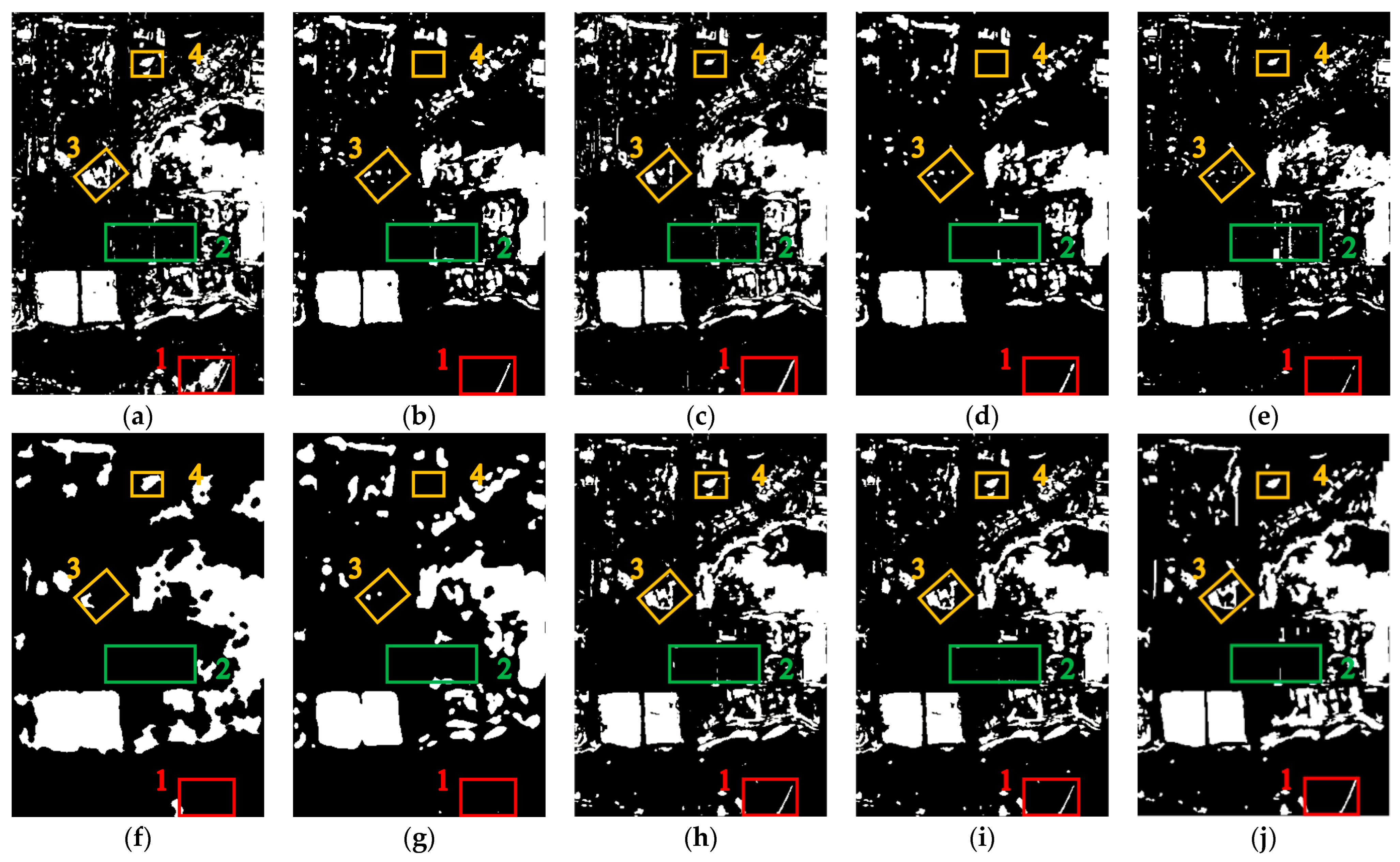
3.3.1. Dataset A

The main types of land cover in dataset A are vegetation, bare land, concrete buildings, sheds, and hardened roads. Factors causing difficulty in change detection include building shadows due to the illumination of the images and radiation differences. In addition, vehicles driving on the roads caused some interference with change detection.

Table 1. Accuracy of different detection methods in dataset A (optimal results in bold).

Method	FA (%)	MA (%)	OA (%)	F1
TCO	3.32	16.72	94.04	0.8463
PCA-K-means	1.73	20.35	94.61	0.8533
ASEA	5.17	18.13	92.28	0.8068
WCIM	2.83	27.35	92.34	0.7889
DSFA	2.42	24.05	93.32	0.8174
DCVA	3.06	18.33	93.93	0.8413
KPCA-MNet	3.19	20.28	93.45	0.8273
LHSP-E	1.17	19.53	95.21	0.8688
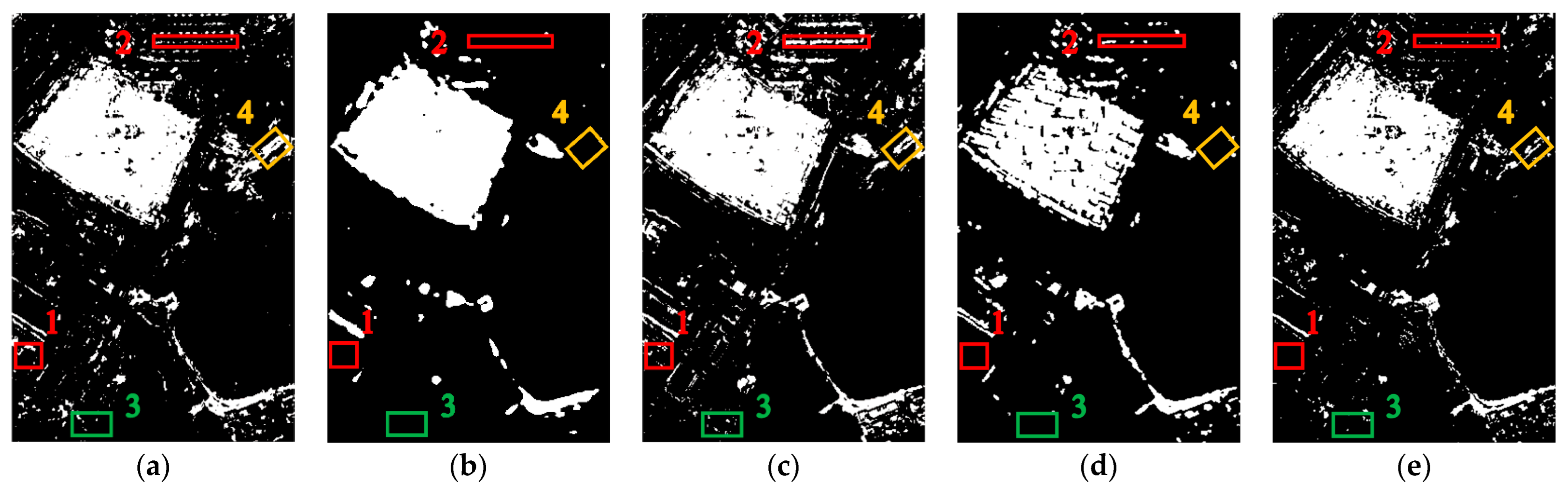
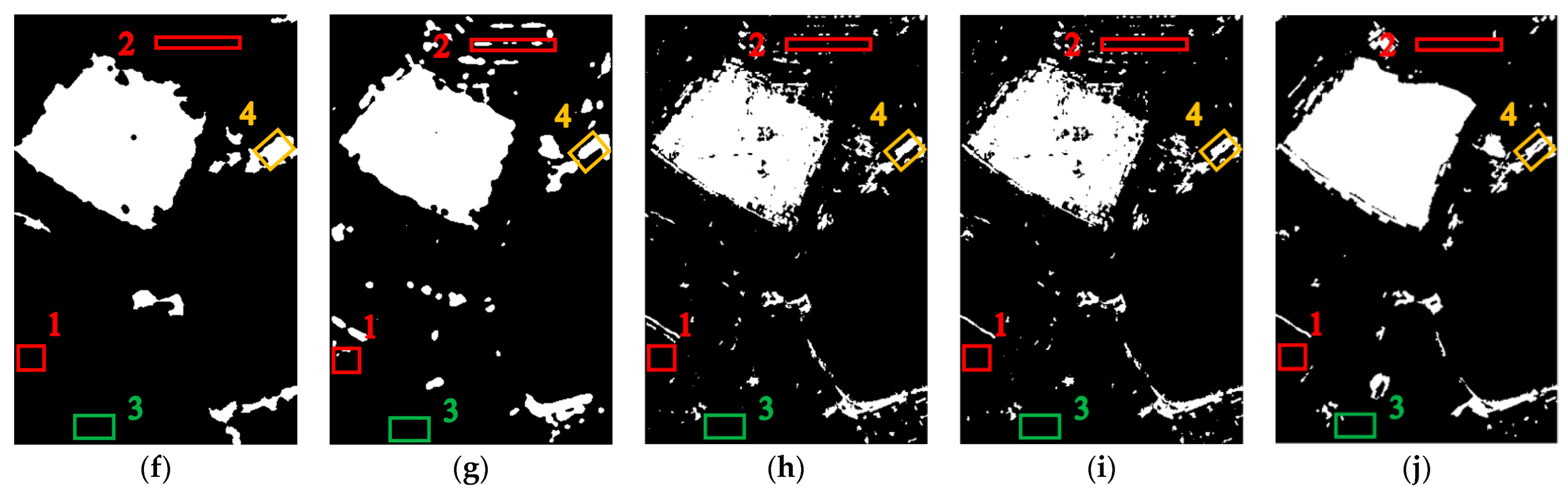
LHSP-C	1.09	19.94	95.20	0.8678

lists the values of the detection accuracy metrics, and Figure 5 shows the change detection results.

As can be seen from Table 1, LHSP achieved the best values in three metrics, namely, FA, OA, and F1. When compared with the TCO, the average result of the three unsupervised change detection methods based on spatial context information (PCA-K-means, ASEA, and WCIM, henceforth termed spatial-context-based approaches), and the average result of the three unsupervised deep-learning-based change detection methods (DSFA, DCVA, and KPCA-MNet, henceforth termed deep-learning-based approaches), the value of FA achieved by LHSP decreased by 2.19%, 2.11%, and 1.76%, respectively. Meanwhile, the OA and F1 increased by 1.17% and 0.0220, 2.13% and 0.0520, 1.64% and 0.0396, respectively. In terms of MA, the TCO achieved the best value, while the value achieved by LHSP is slightly higher than the TCO by 3.02%, but 2.21% and 1.15% lower than that achieved by the spatial-context-based approaches and the deep-learning-based approaches, respectively.

According to Figure 5, the intuitive differences among the different methods are small. The TCO and ASEA methods caused the creation of more false-detection pixels and specks, such as the false-detection pixels caused by illumination of the image in box 1, the false-detection pixels caused by building shadows in box 2, and the specks caused by sporadic differences in vegetation radiation in box 3. The PCA-K-means and WCIM methods produced fewer false-detection pixels and specks but many missed-detection pixels, as in box 4. The DSFA method exhibits many specks and has some missed-detection pixels, as indicated in box 4. The DCVA method performs well in eliminating false-detection pixels caused by building shadows (box 2) but still exhibits missed-detection pixels in detecting changes at the detailed level. The performance of the KPCA-MNet method is similar to that of DCVA, but it still has some false-detection pixels in box 2. The CDIs obtained by LHSP show that our method effectively reduced the number of false-detection pixels and specks (boxes 1–3) and are closer to the reference image (Figure 5j). All methods achieved high detection accuracy in dataset A, but the LHSP method is the best.

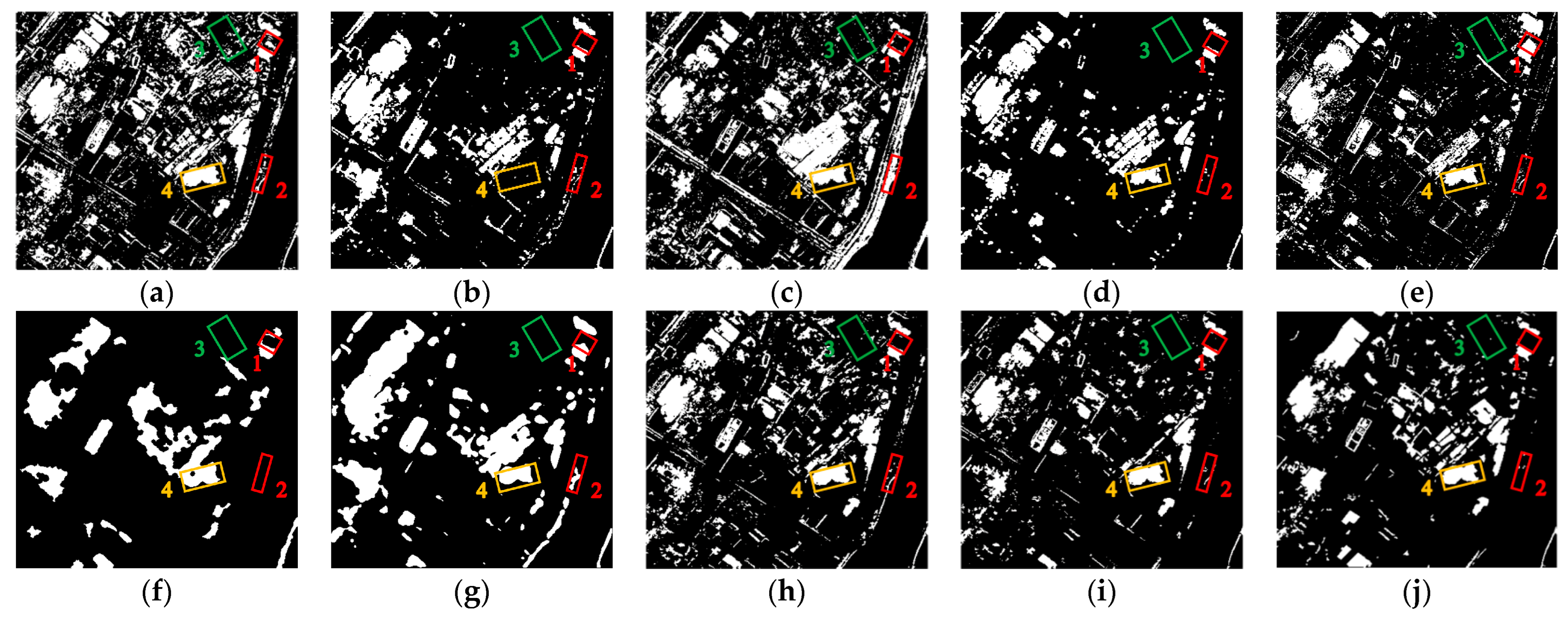
3.3.2. Dataset B

The main land cover types in dataset B are vegetation, bare land, buildings, rivers, and roads. Difficulty in change detection is mainly due to differences in surface radiation caused by illumination of the images and differences in vegetation growth.

The values of the detection accuracy metrics are listed in

Table 2. Accuracy of different detection methods in dataset B (optimal results in bold).

Method	FA (%)	MA (%)	OA (%)	F1
TCO	5.22	10.97	93.55	0.8549
PCA-K-means	3.89	38.04	88.82	0.7028
ASEA	5.14	20.58	91.56	0.8007
WCIM	3.39	40.44	88.71	0.6924
DSFA	2.29	40.41	89.58	0.7093
DCVA	7.27	31.97	87.46	0.6983
KPCA-MNet	4.94	31.72	89.35	0.7323
LHSP-E	2.17	13.99	95.31	0.8867
LHSP-C	1.81	15.21	95.33	0.8856

, and the distribution of the change regions is shown in Figure 6.

As shown in Table 2, similar to its performance on dataset A, LHSP also achieved the best FA, OA, and F1 on dataset B. Specifically, the FA value is 3.23%, 2.15%, and 2.84% lower than that achieved by the TCO, spatial-context-based approaches, and deep-learning-based approaches, respectively. The values of OA and F1 are 1.77% and 0.0313 higher, 5.62% and 0.1542 higher, and 6.52% and 0.1729 higher, respectively, than those achieved by the above methods. For MA, the TCO achieved the best value. The value achieved by LHSP is 3.63% higher than that achieved by the TCO but 18.42% and 20.1% lower than that achieved by the spatial-context-based and deep-learning-based approaches, respectively.

The CDIs obtained by LHSP are closer to the reference image (Figure 6j). The CDIs obtained by the TCO, ASEA, and DSFA have more specks (box 2), and the TCO has obvious false-detection areas due to crop growth (box 1). PCA-K-means and WCIM exhibit many missed detections, such as the changes in vegetation and bare land in box 3 and the changes in the pond and vegetation in box 4. Although DCVA and KPCA-MNet significantly reduced the number of specks, they also led to a considerable increase in missed detections, as evident in box 3 for DCVA and boxes 3–4 for KPCA-MNet. Similarly to dataset A, all methods produced relatively good detection results because of the low detection difficulty in this dataset. However, LHSP still effectively reduced the number of false-detection areas and specks, reduced the missed detection rate, and produced better detection results than the benchmark methods.

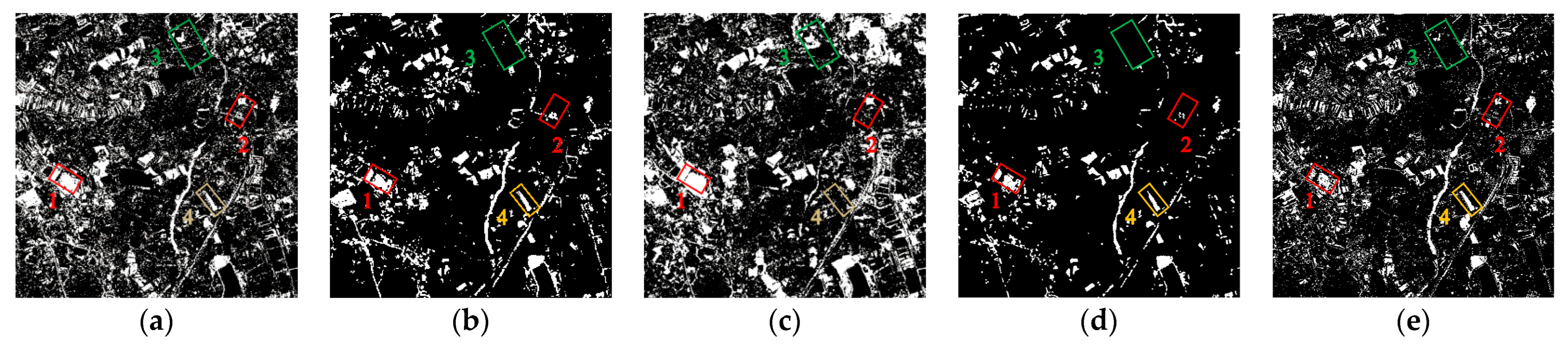
3.3.3. Dataset C

The main land cover types in the bitemporal images in dataset C are farmland, aquaculture water, natural water, sheds, hardened roads, and bare land. Difficulty in change detection in this dataset is mainly due to seasonal differences in crop growth and differences in surface radiation caused by factors such as light conditions and soil moisture, as well as the effect of suspended matter in aquaculture waters, and this dataset is highly susceptible to false detection.

Table 3. Accuracy of different detection methods in dataset C (optimal results in bold).

Method	FA (%)	MA (%)	OA (%)	F1
TCO	15.02	10.85	85.55	0.6256
PCA-K-means	8.15	42.50	87.20	0.5489
ASEA	17.75	22.49	81.61	0.5330
WCIM	5.13	35.42	90.77	0.6545
DSFA	7.13	33.32	89.32	0.6285
DCVA	5.93	46.60	88.56	0.5584
KPCA-MNet	9.03	27.33	88.49	0.6309
LHSP-E	7.39	18.18	91.15	0.7146
LHSP-C	2.79	25.85	94.09	0.7725

lists the values of the detection accuracy metrics, and Figure 7 shows the distribution of the changed areas.

The overall detection accuracy in dataset C is lower than in datasets A and B. Specifically, the average value of F1 achieved by the proposed method and the seven benchmark methods is 0.2057 and 0.1440 lower than in datasets A and B, respectively. The mean value of FA is 6.04% and 4.69% higher than in datasets A and B, respectively.

The quantitative detection results for dataset C follow those for datasets A and B. LHSP achieved the best FA, OA, and F1. When compared with TCO, spatial-context-based approaches, and deep-learning-based approaches, in LHSP, the FA is 9.93%, 5.25%, and 2.27% lower; the OA is 7.07%, 6.09%, and 3.83% higher; and the F1 was 0.1180, 0.1648, and 0.1376 higher, respectively. For MA, the value achieved by LHSP is 11.17% higher than that achieved by the TCO, but it is 11.46% and 13.74% lower than that achieved by the spatial-context-based and deep-learning-based approaches, respectively.

As seen in Figure 7, LHSP achieved reductions of different magnitudes in both false-detection pixels and specks, such as false-detection pixels due to suspended matter in aquaculture water in box 1, false-detection pixels due to radiation differences from vegetation growing near the river in box 2, and specks due to seasonal climate changes in box 3. PCA-K-means produced more missed detection results in dataset C, such as in box 4. The performance of DCVA is similar to its performance on dataset B; that is, despite its significant reduction of specks, its CDI overall has many missed-detection pixels. The overall detection results of all methods are worse for dataset C than for datasets A and B. This is because dataset C contains more pseudo-change information, making detection more difficult. This conclusion can also be derived from comparing the quantitative detection accuracy metrics in Table 1, Table 2 and Table 3. The detection results of LHSP are closest to the reference image (Figure 7j).

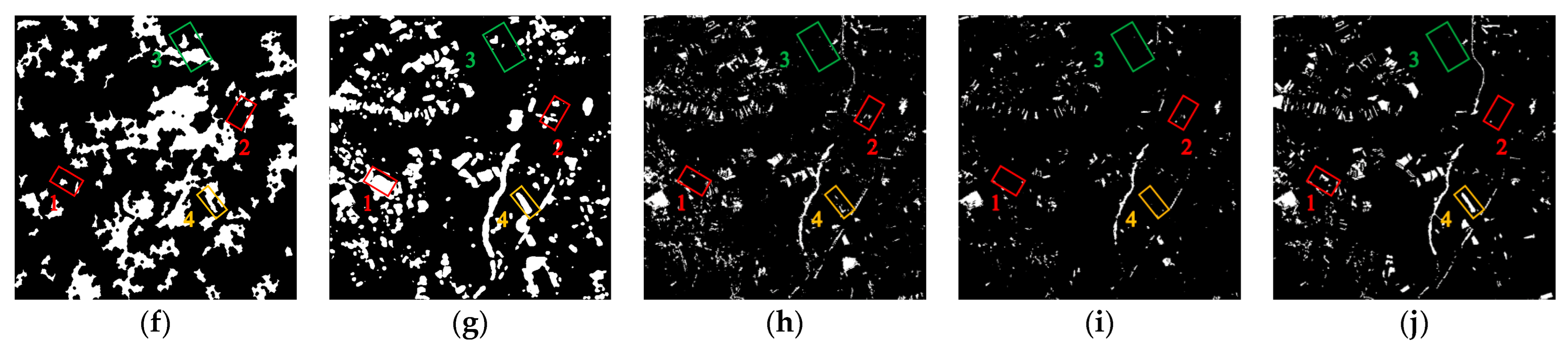
3.3.4. Dataset D

Dataset D comprises images of a more complex area, which includes agricultural land, roads, natural water, buildings, vegetation, aquaculture water, bare land, sheds, and other land cover types. Compared with the previous three datasets, this dataset has more land cover types and change scenarios, and it is also more difficult to detect changes.

Table 4. Accuracy of different detection methods in dataset D (optimal results in bold).

Method	FA (%)	MA (%)	OA (%)	F1
TCO	20.49	6.57	80.25	0.3335
PCA-K-means	7.61	22.10	91.62	0.4960
ASEA	23.73	28.58	76.02	0.2396
WCIM	3.57	31.47	94.95	0.5895
DSFA	9.99	21.31	89.41	0.4402
DCVA	20.76	78.40	76.19	0.0876
KPCA-MNet	13.17	13.95	86.79	0.4080
LHSP-E	2.55	27.66	96.12	0.6634
LHSP-C	0.40	58.79	96.51	0.5552

lists the values of the accuracy metrics, and Figure 8 shows the change regions.

Following the detection difficulty, dataset D has lower values of F1 in comparison with the previous three datasets. The average value of F1 achieved by the proposed method and the seven benchmark methods is 0.4237. LHSP achieved a significant improvement in accuracy over the seven benchmark methods. It achieved the best FA, OA, and F1. Specifically, the value of FA is 19.02%, 10.16%, and 13.17% lower compared to that achieved by the TCO, spatial-context-based, and deep-learning-based approaches, respectively. The OA and F1 are 16.07% and 0.2758 higher, 8.79% and 0.1676 higher, and 12.19% and 0.2974 higher, respectively. The deep-learning-based approaches performed poorly on this dataset because of the unsatisfactory detection results from the DCVA method. LHSP has a higher MA value due to the excessive MA value achieved by LHSP-C, namely, 58.79%. However, LHSP-C still performed better than the seven benchmark methods regarding overall detection.

According to Figure 8, LHSP exhibits remarkable advantages: a reduction in false-detection pixels and specks when compared with the change detection results of the TCO, ASEA, and DSFA (boxes 1–3) and a reduction in the overall false detection rate when compared with the change detection results of PCA-K-means and KPCA-MNet (box 1). The CDI for WCIM is better, but there are still a few false-detection pixels (box 1). The CDI of DCVA has many false-detection and missed-detection pixels. LHSP still maintained higher accuracy than the benchmark methods, although it also suffers from more missed-detection pixels (box 4). The LHSP-E results are closest to the reference image (Figure 8j).

Compared to the seven benchmark methods, LHSP shows a greater improvement in accuracy in datasets C and D than the improvement observed in datasets A and B. The average value of F1 achieved by LHSP is 0.0935 higher than that achieved by the seven benchmark methods in datasets A and B, while it is 0.1926 higher in datasets C and D. LHSP exhibited more obvious advantages in terms of the accuracy of change detection in HR RS imagery with a more complex landscape.

The experimental results showed that LHSP has higher detection accuracy than the seven benchmark methods in all four datasets. The average difference in the four accuracy metrics FA, MA, OA, and F1 between LHSP and the seven benchmark methods is −5.48%, −2.97%, 5.95%, and 0.1430, respectively. Moreover, LHSP reduced the number of specks and false-detection pixels to a certain extent.

4. Discussion

The LHSP method consists of a local XCS-LBP histogram similarity measure, the proposed POTSU segmentation method, and the segmentation of the SCV using the active contour model. The local XCS-LBP histogram similarity measure incorporates spatial information into change detection. The POTSU segmentation method further reduces the false detection rate in change detection in HR RS imagery. The SCV segmentation using the active contour model improves detection accuracy by combining spectral and spatial information.

Below, we further discuss and analyze the validity of the method. Finally, the runtime is discussed and compared.

4.1. Validity of Local XCS-LBP Histogram Similarity

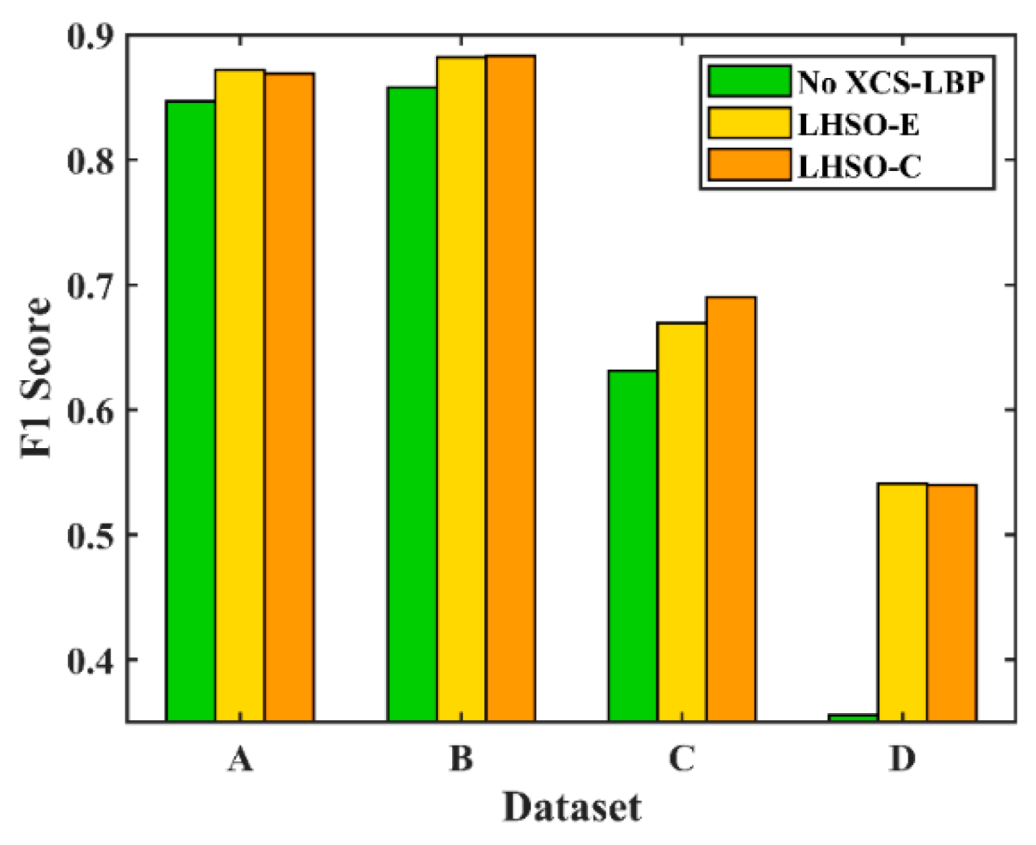
The SCV and local XCS-LBP histogram similarity were used as input features, respectively. The initial results were obtained by segmentation using the Otsu method and were then used as seeds in the active contour model to segment the SCV to produce the final results. Figure 9 shows the accuracy of change detection.

No XCS-LBP in Figure 9 indicates SCV input, while LHSO-E and LHSO-C indicate XCS-LBP input, where E and C indicate that the histogram similarity was calculated using the Euclidean distance and chi-squared distance, respectively. The F1 values achieved using XCS-LBP input in all datasets are higher than those achieved using SCV input, which indicates the effectiveness of XCS-LBP in LHSP.

A comparison of the detection results (Table 1, Table 2, Table 3 and Table 4) of PCA-K-means, ASEA, WCIM, and LHSO (Figure 9) on the four datasets shows that LHSO exhibits the highest detection accuracy on all datasets except for dataset D, where it is lower than that of WCIM. The F1 value achieved by LHSO in the four datasets is 0.0173, 0.0822, 0.0255, and −0.0491 higher, respectively, than the highest F1 value achieved by PCA-K-means, ASEA, and WCIM. This indicates that combining spatial context information from XCS-LBP with spectral information in change detection is more effective when compared with PCA-K-means, ASEA, and WCIM, which directly use spatial context information based on the original grayscale values.

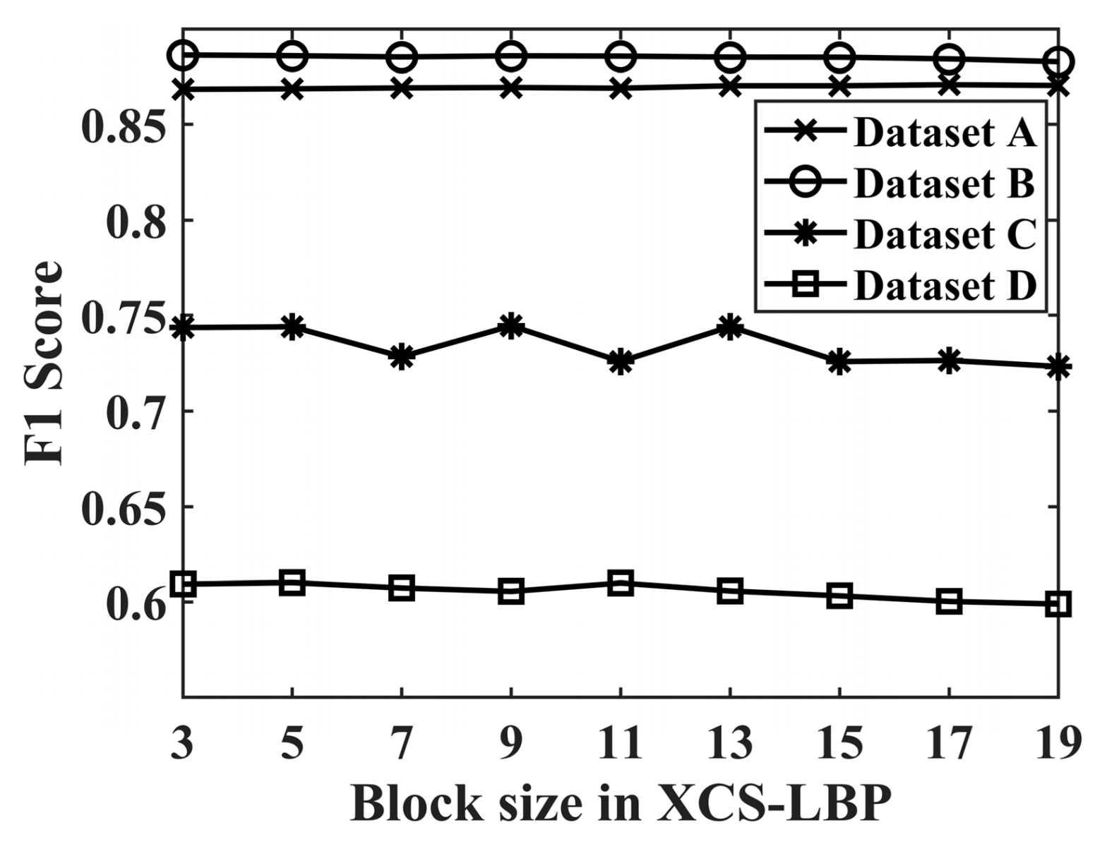
To verify the reasonableness of block size in XCS-LBP, 3 × 3, 5 × 5, $\cdots$, and 19 × 19 were used as the sizes of the local blocks in XCS-LBP extraction. The mean values achieved by LHSP-E and LHSP-C were compared, and the results are shown in Figure 10.

As can be seen in Figure 10, LHSP is not sensitive to the block size in XCS-LBP. Datasets A, B, C, and D achieved optimal F1 at 17 × 17, 3 × 3, 9 × 9, and 5 × 5, respectively. This is affected by the image’s spatial resolution and the land cover. Although datasets A, C, and D did not achieve the optimal F1 at 3 × 3, F1 is only 0.0024, 0.0009, and 0.0008 lower than the optimal F1, respectively. The insensitivity of LHSP to block size in XCS-LBP is due to the mechanism by which XCS-LBP expresses spatial information and the effect of regional growth. For convenience, 3 × 3 is used as the block size in XCS-LBP for all four datasets.

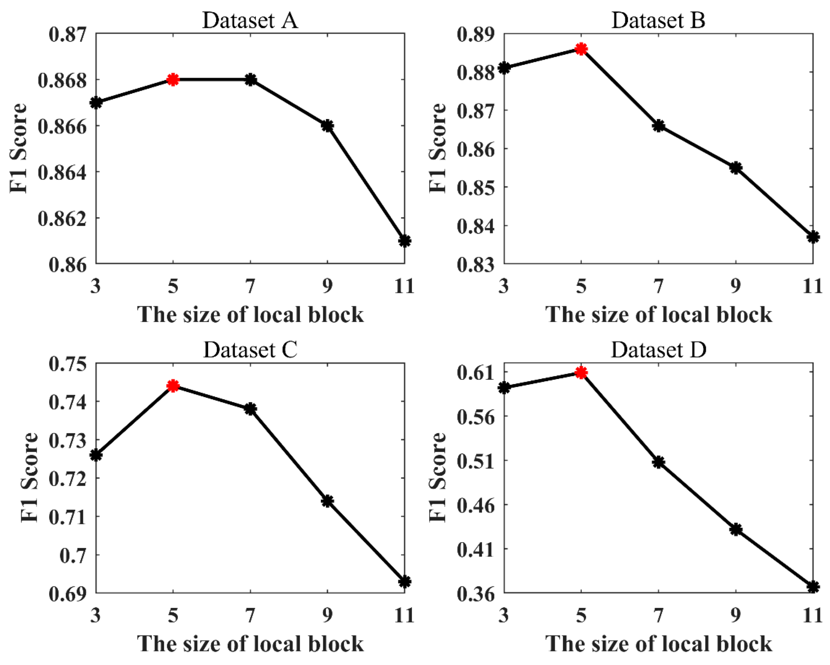
Co-registration errors were considered when determining the range of the histogram construction. Also, to verify the reasonableness of its size, 3 × 3, 5 × 5, $\cdots$, and 11 × 11 were used as the sizes of the local blocks in the construction of the histogram in LHSP. The mean values achieved by LHSP-E and LHSP-C were compared, and the results are shown in Figure 11.

Figure 11 shows that the F1 value in all four datasets increases at first and then decreases when the local block becomes larger, and the best F1 value is achieved at a block size of 5 × 5. Therefore, this confirms the reasonability of choosing a block size of 5 × 5.

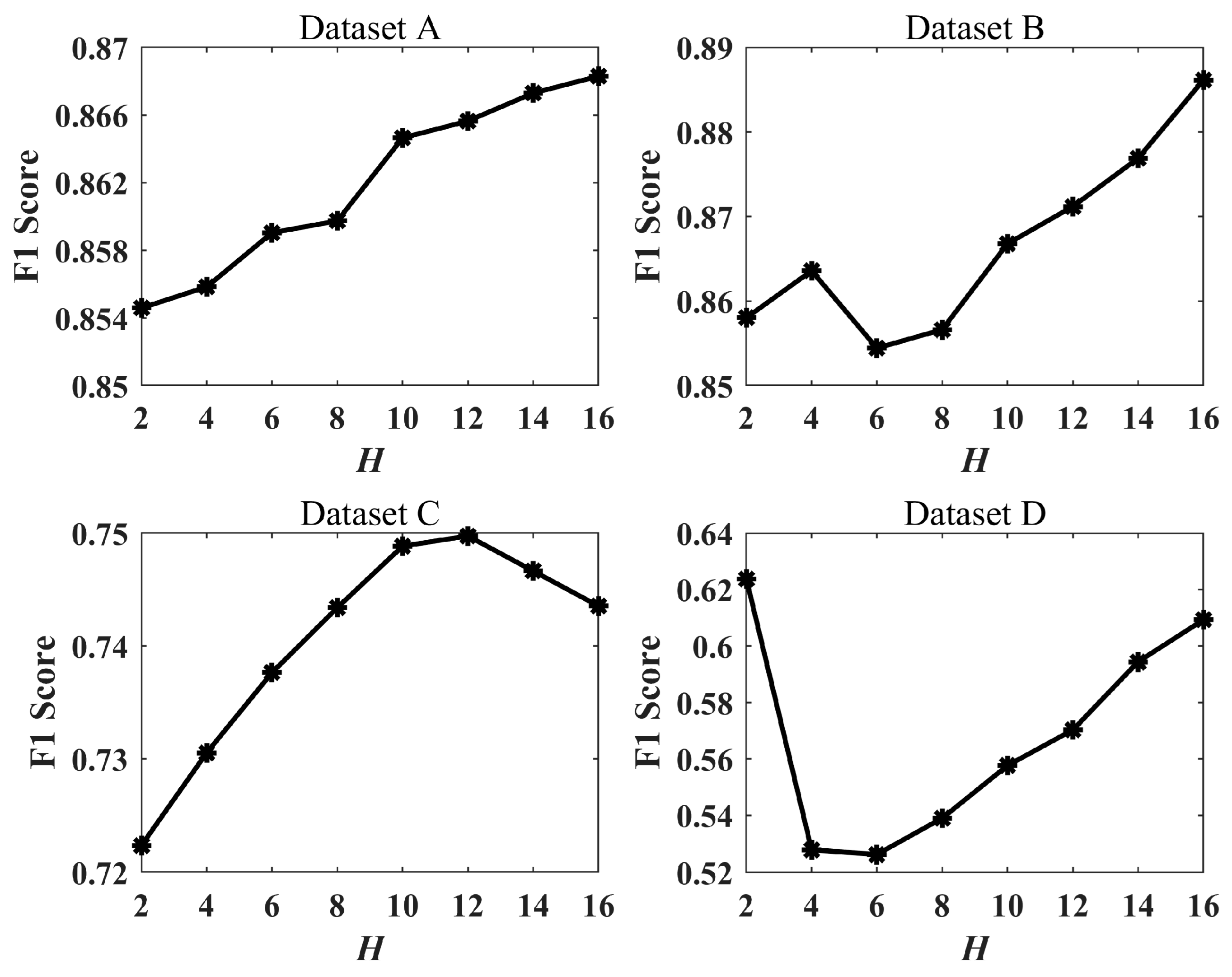
In addition, we performed change detection using LHSP with different bins (H) and compared the detection accuracy to analyze the effect of H on the detection results, as shown in Figure 12.

As shown in Figure 12, the F1 have slight variations with H in all four datasets. For dataset A, the F1 continue to improve as H increases. For dataset C, the F1 show an increase followed by a decrease. However, for dataset B and dataset D, the F1 fluctuate when H is small and continue to improve. Overall, the F1 climbed gradually as H increased, thus indicating that our histogram construction using 16 columns is effective.

Similarly, different LBP variants can affect the detection results. To validate the effectiveness of XCS-LBP in LHSP, traditional LBP (TLBP) [56] and rotation-invariant LBP (RLBP) [56,57] were used to replace XCS-LBP for change detection, respectively. The comparison results are shown in

Table 5. Relationship between F1 score and different variants of LBP (optimal results in bold).

Variants	A	B	C	D
TLBP	0.8633	0.8593	0.7340	0.4794
RLBP	0.8622	0.7782	0.7919	0.5284
XCS-LBP	0.8683	0.8862	0.7436	0.6093

.

The results show that XCS-LBP has lower F1 than RLBP in dataset C, but it achieves the best F1 in datasets A, B, and D. Overall, XCS-LBP outperformed LBP and RLBP in LHSP.

4.2. Validity of POTSU Segmentation

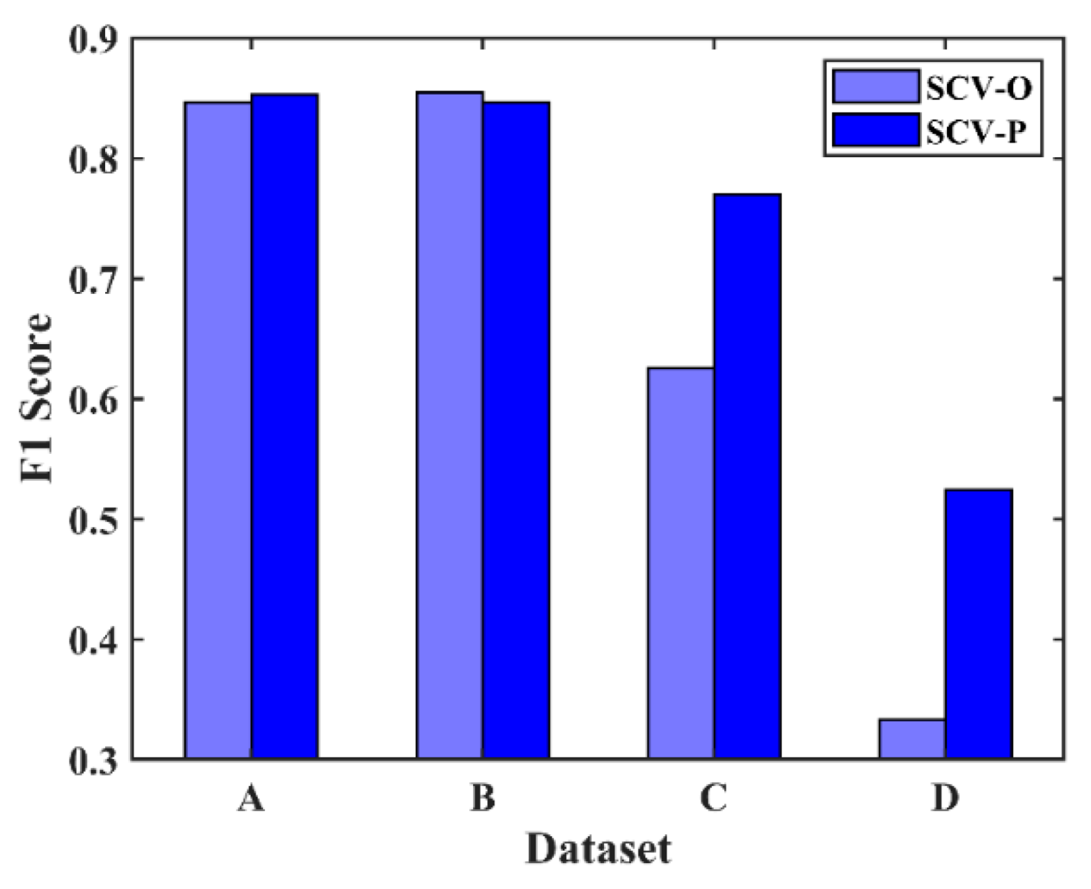
Three experiments were performed to verify the effectiveness of the proposed POTSU method. In experiment 1, the SCV was the input image feature and was segmented directly by the Otsu method and POTSU. The result is shown in Figure 13.

SCV-O in Figure 13 denotes SCV segmentation by the Otsu method, while SCV-P denotes SCV segmentation by the proposed POTSU method. The F1 values achieved by POTSU are higher than those achieved by the Otsu method in datasets A, C, and D. The differences are evident in the complex datasets C and D. The fact that the differences in the value of F1 in datasets A and B are minor is because segmentation by the Otsu method can also achieve good results for simple images. In general, POTSU is more suitable than the Otsu method for segmentation in change detection in HR RS imagery, and the superiority of POTSU in terms of accuracy is more obvious in complex HR RS data.

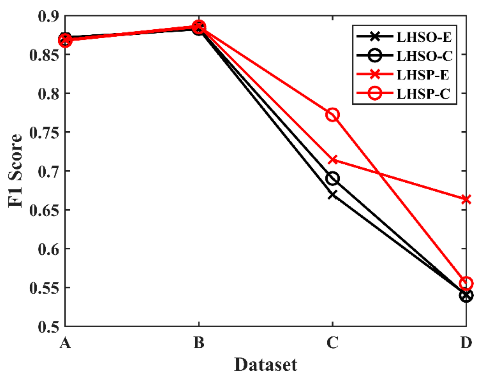
In experiment 2, POTSU was substituted with the Otsu method in LHSP (i.e., to give LHSO) to verify the effectiveness of POTSU in LHSP. The result is shown in Figure 14.

As seen in Figure 14, the differences in the value of F1 are minor for the simple datasets A and B, whether the histogram similarity was measured using the Euclidean or chi-squared distance. However, LHSP achieved better detection results in the more complex datasets C and D.

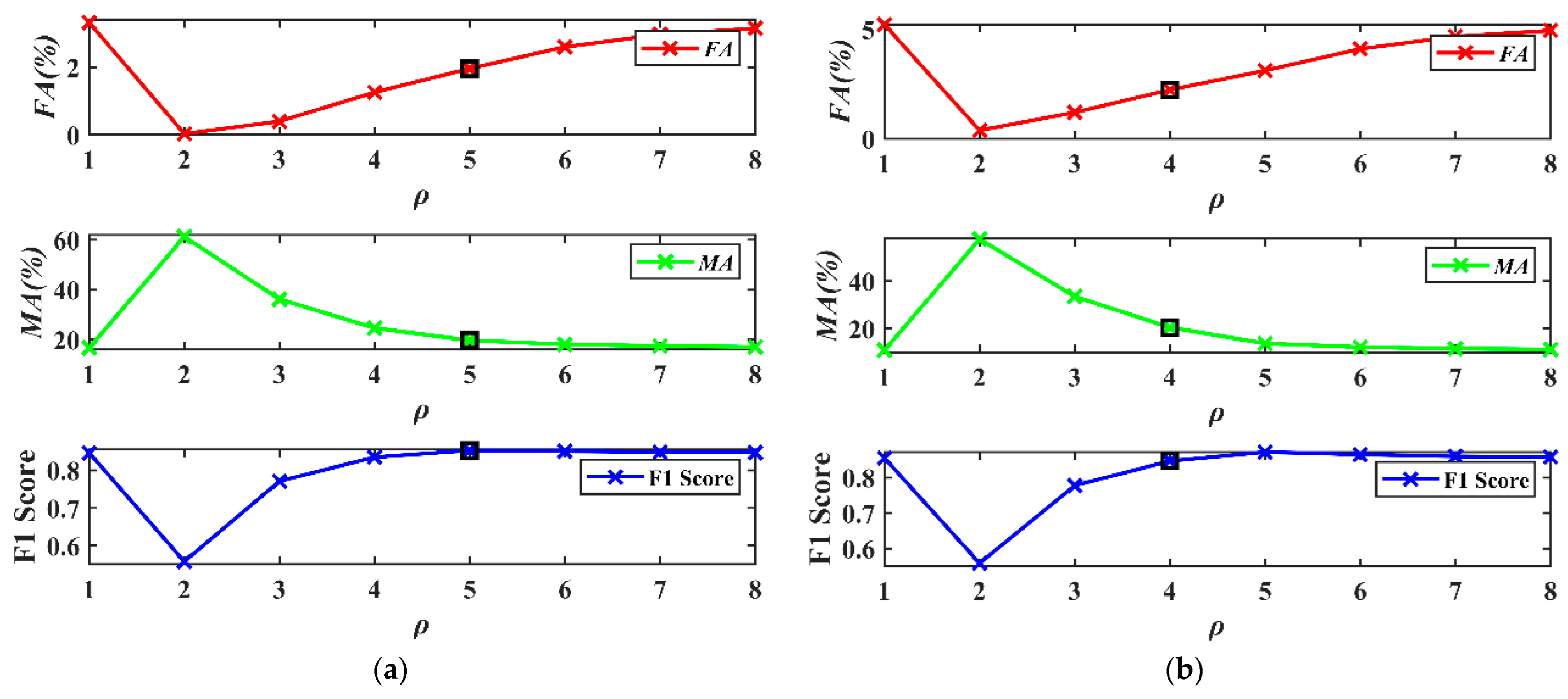
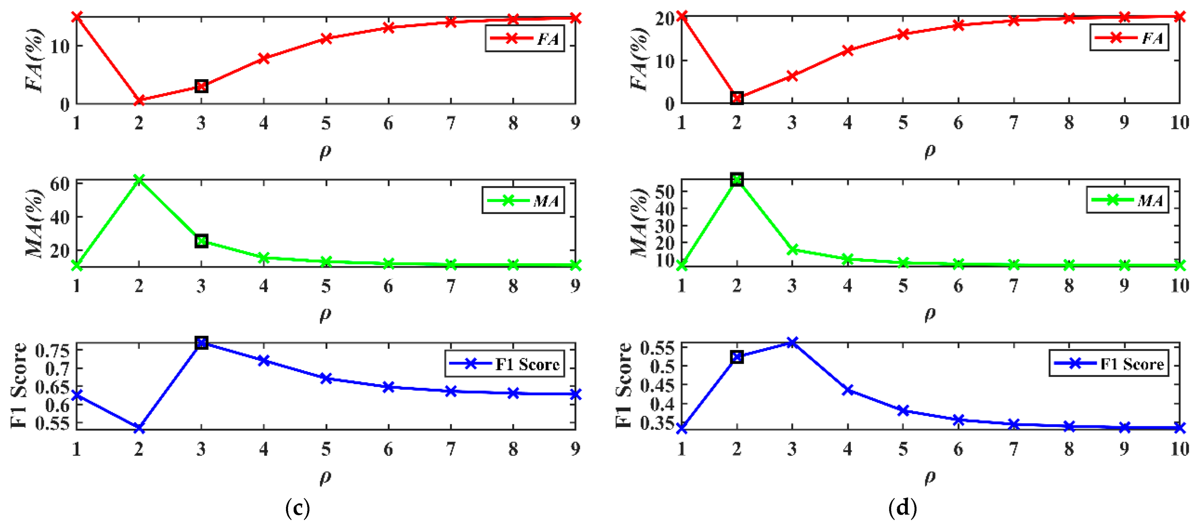
In experiment 3, POTSU uses $ndi$ and $ndj$ to determine that the segmented objects in the progression are validated. The SCV was the input image feature and was segmented directly by the POTSU, and then the FA, MA, and F1 obtained from each progression were analyzed, as shown in Figure 15.

In Figure 15, the values of FA all decrease first and then gradually increase, and the values of MA increase first and then decrease. This variation aligns with our explanation of using $ndi$ and $ndj$ in POTSU to determine segmented objects. Specifically, Otsu usually has a high false detection rate for complex HR data change detection (red line when the number of progressions is 1). The false detection rate decreases sharply after POTSU continues to segment the changed pixels from the last progression (red line when the number of progressions is 2). Still, the missed detection rate increases dramatically simultaneously (green line when the number of progressions is 2), so POTSU continues to judge the segmented objects to gradually balance the false detection and missed detection until the termination condition is reached. Finally, POTSU selects the final progressive result based on the maximum difference between $nadj$ and $nadi$ of each progressive merge result.

In this experiment, the 5th, 4th, 3rd, and 2nd progressive results were selected as the final results for datasets A, B, C, and D, respectively (small black box in Figure 15). It can be observed that the small black box is overall in the moderate position of FA and MA, thus avoiding too big or too small values of FA and MA. However, this is not the case for dataset D. This is because the mask segmentation makes the accuracy obtained from each progression not continuous, so it is difficult to ensure that the result is optimal each time (such as the final F1 of datasets B and D being suboptimal).

Nevertheless, POTSU effectively takes the optimal range of values (such that datasets A and C achieve the optimal values while datasets B and D achieve the suboptimal values), so POTSU has good accuracy improvement overall. It can also be seen that on the relatively simple datasets A and B, the F1 does not improve significantly. Still, on the more complex datasets C and D, the F1 of POTSU shows a significant improvement relative to Otsu.

The results of these three experiments show that the proposed POTSU method has an advantage over the Otsu method in change detection in HR RS imagery, which is more evident in the case of more complex HR RS imagery.

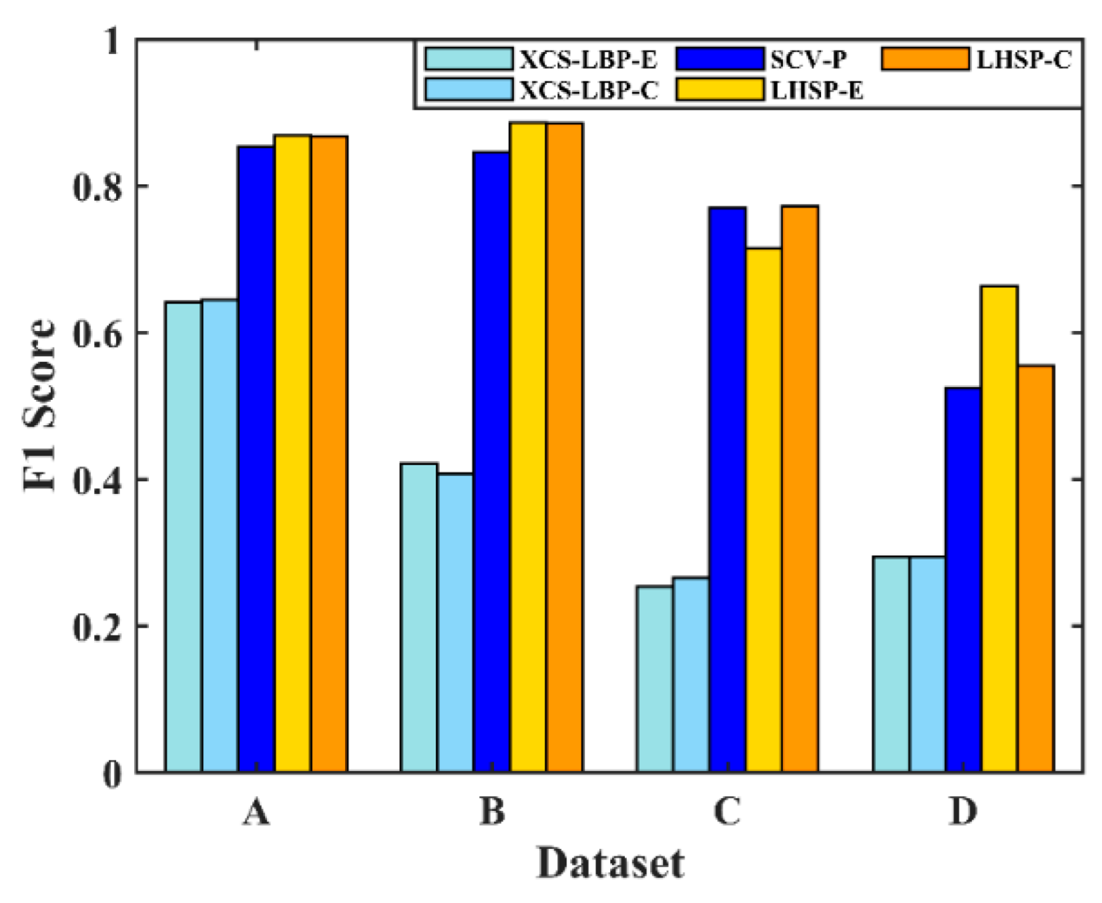
4.3. Validity of Combination of Spectral and Spatial Information

Three comparative experiments were conducted: (1) spectral information only; the SCV was segmented directly, which is denoted as SCV-P; (2) spatial context information only; the segmentation of the two CVs of the XCS-LBP features is denoted as XCS-LBP-E and XCS-LBP-C, respectively; (3) spectral information and spatial context information were combined; region growth was performed with the SCV based on experiment (2), which is denoted as LHSP-E and LHSP-C, respectively. All the segmentations were implemented using POTSU. The results are shown in Figure 16.

It can be seen from Figure 16 that the accuracy of change detection with spatial information alone is low because of the lack of description of spectral-dimensional information in the representation of pixel features. Similarly, the accuracy of change detection with spectral information alone is relatively low because the description of spatial context information is ignored. However, the value of F1 with spectral information alone is significantly higher than that with spatial information alone. The proposed LSHP exhibits higher detection accuracy because of the combination of spectral and spatial information. Specifically, it has a slight advantage over SCV-P in datasets A and B in terms of accuracy. This is because simple change scenario information can also be well characterized using spectral information alone. For dataset C, the proposed method has similar detection accuracy to SCV-P, which is due to the superior performance of POTSU in dataset C (Figure 13). However, for dataset D, the proposed method achieved a larger increase in the value of F1, namely, 8.47%. This is because spectral information alone cannot represent changes in various land cover types well for dataset D, which contains complex change scenarios. In contrast, adding spatial information enhanced the performance in this respect. The initial change detection implemented in LHSP using only spatial information gave a suitable seed for the regional growth of SCV and showed good detection results.

4.4. Runtime Analysis

The runtime is an important metric for evaluating the effectiveness of an algorithm.

Table 6. Runtimes of different methods.

Method	A (s)	B (s)	C (s)	D (s)
TCO	0.08	0.08	0.09	0.12
PCA-K-means	1.21	1.23	1.73	4.54
ASEA	21.65	21.37	27.40	57.18
WCIM	6.85	6.53	8.33	16.32
DSFA	11.54	10.64	10.93	13.68
DCVA	8.86	10.16	10.94	20.14
KPCA-MNet	7.56	7.52	10.77	21.33
LHSP-E(POTSU)	13.58 (0.23)	14.45 (0.31)	18.44 (0.36)	35.69 (0.64)
LHSP-C(POTSU)	9.01 (0.24)	9.37 (0.25)	12.07 (0.34)	22.78 (0.58)

lists the runtimes of each method.

Table 6 shows that the average running speed of each method from fast to slow is as follows: TCO > PCA-K-means > WCIM > DSFA > KPCA-MNet > DCVA > LHSP-C > LHSP-E > ASEA. The TCO took the shortest time because it only required SCV calculation and single threshold segmentation. The runtime of PCA-K-means is also short. This is because PCA took less time since HR RS images used only included four bands and K-means only performed two-class clustering. However, the missed detection rate of PCA-K-means is more serious. The running time of WCIM is increased compared to TCO and PCA-K-means methods because it took some time to calculate the weights of each band. DSFA, KPCA-MNet, DCVA, and LHSP-C have minor differences in runtime. The time consumed by LHSP is mainly dedicated to extracting XCS-LBP features. The time taken for POTSU is very short (shown in parentheses in Table 6), though it took more time than the TCO because more processing is required. LHSP-E is slightly more time-consuming than LHSP-C because calculating Euclidean distances takes longer. ASEA is relatively time-consuming, mainly because ASEA requires adaptive region generation for each pixel, and the traversal is more time-consuming.

Overall, when compared with the runtimes of the benchmark methods, the time taken by LHSP is acceptable, considering the improvement in detection accuracy.

5. Conclusions

This study developed an unsupervised method for detecting land cover changes in HR RS imagery by combining spatial context information (expressed by the local XCS-LBP) with spectral information (expressed by the SCV) and a POTSU threshold segmentation method.

The effectiveness of the proposed method was verified by a comparison with the TCO, PCA-K-means, ASEA, WCIM, DSFA, DCVA, and KPCA-MNet based on four sets of bitemporal HR RS images with different spatial resolutions and landscape complexities.

(1) The proposed method effectively reduced the number of false-detection pixels and achieved higher detection accuracy than the benchmark methods. In the test datasets, the mean F1 score achieved by the proposed method is 0.0955 higher than the highest mean F1 score achieved by the benchmark methods;

(2) Compared with the Otsu method, the proposed POTSU method exhibited better segmentation performance in change detection in complex HR RS imagery;

(3) The proposed method is suitable for land cover and land use mapping. In addition, it has detection advantages for HR RS images with complex land cover and high detection difficulty.

In the future, we plan to work on (1) exploring methods to handle co-registration errors based on XCS-LBP and (2) integrating the proposed POTSU with deep learning to enhance detection accuracy further.