1. Introduction
In accordance with the findings from the United Nations Human Settlements Programme (UN-Habitat) report, as of 2023, 56% of the global population resided in urban areas. It is expected to increase by 72% by 2050 [
1]. Cities have entered a large-scale construction and expansion stage, bringing challenges to their operation and development. The construction activities inevitably cause changes in the urban geological environment, potentially inducing geological disasters and causing loss of life and property. Therefore, it is vital to monitor the stability of ground surfaces and artificial infrastructures in a built environment, to capture abnormal deformation signals in a timely manner, and to provide guidance for urban planning and sustainable development. Abnormal deformation refers to non-uniform spatial deformation, a trend of uplift or subsidence, or accelerated changes, indicating the unstable condition of the Earth’s surface or the objects on it.
Synthetic aperture radar (SAR) interferometry (InSAR) [
2] uses radar phase observation to estimate the surface displacements over a large area. Time series InSAR technology [
3,
4,
5,
6,
7] uses coherent point targets that provide reliable phase observation over the long term to extract precise displacements. Multi-epoch InSAR technology has significantly developed over the past three decades [
8,
9,
10,
11,
12]. This efficient monitoring technique has been successfully productized, as demonstrated by services like the European Ground Motion Service (EGMS) [
13] and the Ground Motion Service Germany (BBD) [
14].
The availability of multi-platform, multi-band SAR data, along with increasingly mature time-series InSAR processing schemes, allows us to obtain a large number of InSAR deformation observations. Yet, interpreting these InSAR deformation signals in complex urban scenarios presents a challenge. The selected coherent point targets of the multi-epoch InSAR technique in urban scenes originate from various sources, such as roads, building walls, and roofs. Consequently, the deformation types represented by these observations are diverse. Moreover, the displacement signals observed by InSAR are often mixed, possibly due to ground subsidence or structural instability, thermal expansion of construction materials, atmospheric delay, and noise. This could lead to deformation signals of the targets being submerged in noise, especially when the signal magnitude is small. Finally, urban scenes often contain millions of coherent points, making it challenging to interpret each point individually.
One strategy to address this issue is establishing a link between the InSAR point targets and the ground object [
15,
16,
17]. This is achieved through high-precision 3D positioning [
18,
19], which helps distinguish deformation from different targets, such as ground surfaces or buildings [
20]. Once the types of coherent points are identified, the differences in motion states among them can be used to determine deformation types, such as shallow compaction deformation, building deformation, and deep compaction deformation [
20]. Another strategy is a data-driven approach that attempts to classify the InSAR displacements [
21,
22,
23,
24,
25,
26,
27] or decompose the source among InSAR displacements [
28,
29,
30,
31]. The deformation classification methods include hypothesis testing of time series displacements [
21,
23], unsupervised time series displacements clustering, and deep learning-based deformation identification using extensive training data [
24,
25,
26]. Unsupervised clustering techniques do not necessitate any prior data of the study area and have proven effective at detecting potential deformations in urban environments [
22,
27,
32]. The decomposition methods aim to separate InSAR deformation into multiple components using techniques such as principal component analysis (PCA) or independent component analysis (ICA). These techniques help interpret deformations that originate from distinct physical events tied to different components [
33,
34,
35,
36]. Additionally, the decomposition method can reduce the impact of noise, which in turn improves the clarity of the primary signal elements in InSAR deformation [
32].
This study delves into interpreting mixture deformation signals extracted with the InSAR technique within urban settings by combining signal decomposition approaches and unsupervised clustering methods. The decomposition method extracts deformation source components from InSAR time series displacements. In urban scenarios, deformation is typically mixed and often of small magnitude, making it difficult to identify primary behaviors. The decomposition method assists in this task. The clustering method identifies deformation series with similar characteristics. Thus, an unsupervised processing strategy that combines signal decomposition and clustering methods was established. This strategy automatically recognizes the spatiotemporal characteristics of deformation signals in urban scenarios, offering a powerful tool for monitoring and managing infrastructure stability and urban development. By harnessing advanced clustering and decomposition techniques, it provides insights into the intricate dynamics of urban deformation, enabling timely interventions to mitigate potential risks.
In the experiment, the focus was on the urban area of Kunming City (KMC) in the southwest of Yunnan Province, China. It serves as a point of connection between China, South Asia, and Southeast Asia. In recent years, it has entered a stage of rapid development. C-band, X-band, and L-band data from Sentinel-1, TerraSAR-X, and ALOS-2 PALSAR-2 acquired between 2017 to 2022 were collected. The time-series InSAR analysis is used on these three datasets to estimate the deformation in the KMC. The deformation signals in the three datasets were then compared, and several areas with abnormal deformation were analyzed. Following this, an unsupervised learning method was applied to the InSAR deformation series, enabling the identification of a spatio–temporal deformation feature distribution over KMC. The effectiveness and feasibility of employing the decomposition method for InSAR deformation signals is the focus of the discussion, with the goal of gaining an understanding of the time series displacements in an urban environment. Furthermore, investigation will be conducted into whether the unsupervised method can effectively identify key features across datasets within the same area.
This paper is structured as follows:
Section 2 describes the research area and the data.
Section 3 outlines the methods used.
Section 4 presents the results and discussion, and
Section 6 concludes the study.
2. Study Area and Data
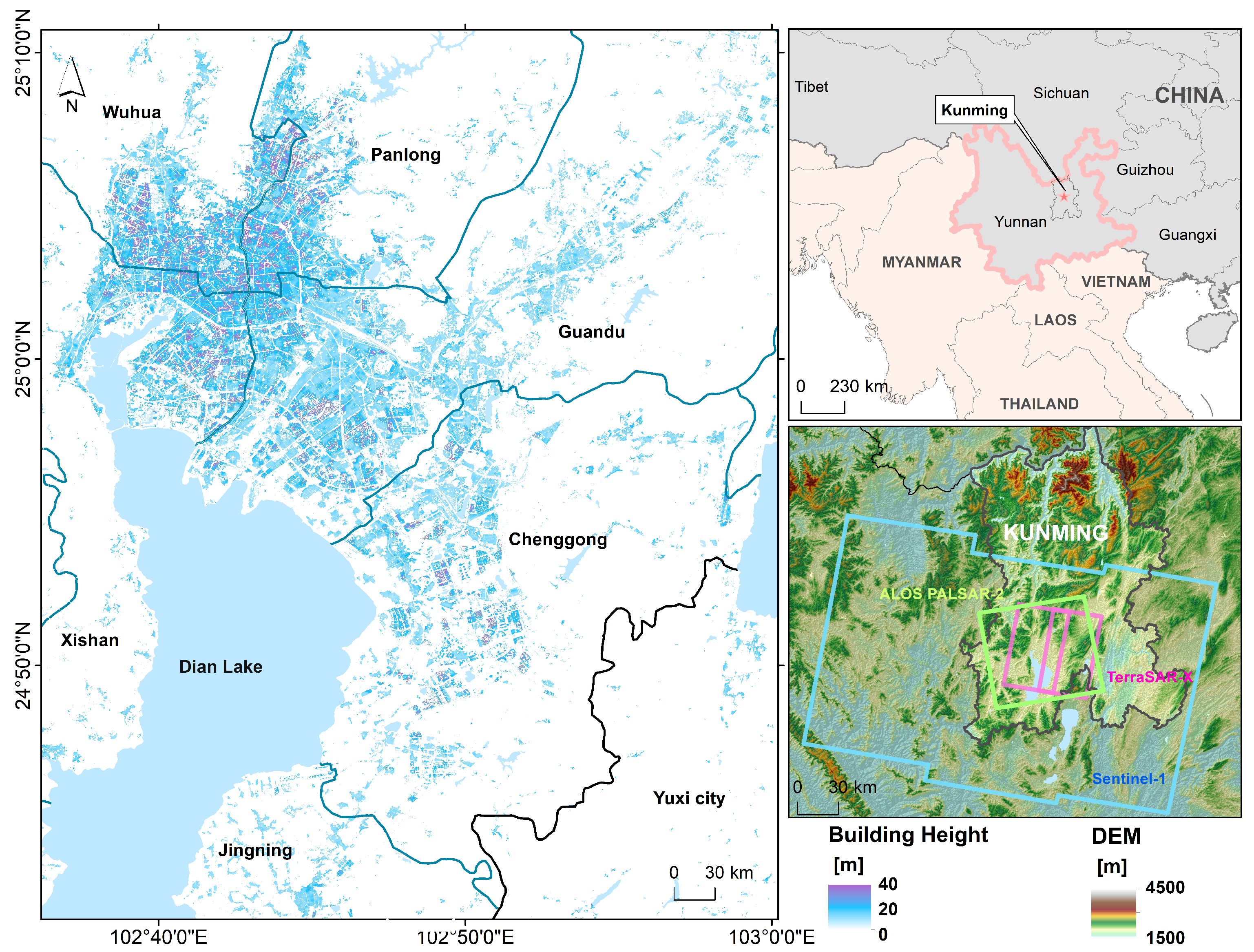
This study focuses on the densely populated areas within Kunming City (KMC), the capital of Yunnan Province in southwestern China, as depicted in
Figure 1. The building heights within KMC, provided by the CNBH-10 product [
37], are illustrated in
Figure 1. Areas with a high concentration of buildings, namely Wuhua District, Panlong District, Guandu District, Chenggong District, and Jinning District, are of particular interest. Most of these buildings are located in the Dianchi Lake basin.
Figure 1 shows KMC’s geographical location in China, its topography, the extent of data collection, and the building heights.
C-band, X-band, and L-band SAR data stacks were collected for the study area. These include 168 Sentinel-1 Interferometry wide (IW) images acquired from January 2017 to December 2022 in descending track with VV polarization, 106 TerraSAR-X Stripmap (SM) images acquired from January 2017 to August 2019 in descending track with HH polarization, and 13 ALOS-2 PALSAR-2 fine mode images acquired from February 2017 to January 2022 in ascending path with HH polarization. The data parameters are provided in
Table 1. The Sentinel-1, TerraSAR-X, and ALOS-2 PALSAR-2 satellites have respective range spacing sizes of 2.33 m, 0.91 m, and 4.29 m. Their azimuth spacing sizes are 13.97 m, 2 m, and 3.40 m, respectively.
3. Methods
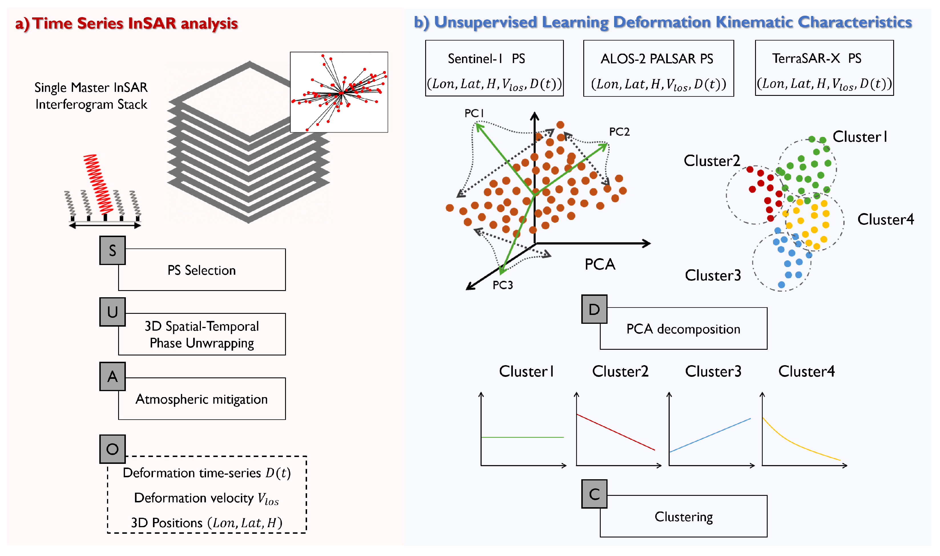
The workflow of this study is illustrated in
Figure 2. There are two main parts: the time series InSAR analysis in
Section 3.1 and the unsupervised learning based InSAR deformation time series interpretation in
Section 3.2.
3.1. Time Series InSAR Analysis
Here, a short description of time series InSAR analysis is given; the details can be referred to in [
5]. The time series InSAR technique uses a group of multiple SAR images to estimate Earth’s surface displacements. Interferograms are generated following a rule of baseline configuration among the SAR images. Coherent points, namely persistent scatterers (PS), are selected for phase analysis. The deformation information is estimated along with the height under an assumption of deformation behavior on each PS.
Supposing there are two PSs
i and
j in two images
m and
s, the corresponding phase observations are
. The interferometric phase between images
m and
s after correcting for geometric terms of the point
i is
The double difference in interferometric phase observation per arc between the two points
i and
j is
where
is modulo-
wrapping operator,
a indicates the integer number of phase ambiguity,
is the displacement phase,
is the topographic phase,
is the orbital phase,
is the atmospheric phase, and
is the noise phase.
The
is the topographic phase due to the residual height difference between point
i and point
j and is given by
where
is the wavelength,
is the perpendicular baseline between
m and
s,
r is the range to the antenna,
is incident angle, and
is the residual height. Assuming
, the residual height
can be estimated. Thus, the height estimation of each PS is related to one selected reference point.
The displacement component is modeled by a function of the temporal baseline
between
m and
s,
The most common model is the linear deformation model, given by
The estimated velocity v is relative to the reference point. Usually, a stable point with the highest coherence value is selected as the reference point.
The atmospheric variation between points i and j in m and s images is given by . The noise term and decorrelation term are summarized in . A spatio–temporal filter eliminates noise and atmospheric components. The errors and uncertainties in the orbit induce errors that are propagated in the calculation of the flat-earth phase. These residual phase components are called orbital phase , which could be estimated with a phase ramp in the interferogram.
The estimated vector of each PS is [va] with a linear deformation model. After estimating the parameters, the time series displacements could be estimated with the by removing the contribution of atmospheric, residual topographic phase, and orbital components.
3.2. Unsupervised Learning Based InSAR Deformation Time Series Interpretation
This section presents principal component analysis (PCA) and the k-means clustering method for exploring deformation series within an unsupervised learning context. PCA identifies the primary features of the deformation time series, whereas the k-means method detects deformation series with similar kinematic characteristics. The goal is to interpret deformation over the urban scene unsupervised.
The PCA method, which can be seen as a strategy for decomposing mixed signals, is essentially a form of the blind signal separation (BSS) process.
The mixed signals can be described as
where
is a row vector containing deformation mixtures,
is the unknown components, and
is the coefficients matrix that describes the contribution of each component to the mixed signals. The unknown components can be recovered with the unmixing matrix
by
The goal of principal component analysis (PCA) is to estimate the mixing matrix
and the component signal
by observing
. PCA primarily focuses on the variance of the signal [
38], aiming to identify components that explain the maximum variance in the data. It seeks to find a set of new, orthogonal components with the maximum variance and is uncorrelated. These components are usually not independent, and each is a linear combination of the original features.
The PCA process typically includes three steps [
39]: First, the observed signal is decentered. Then, based on the decentered signal, its covariance matrix is calculated to compute eigenvalues and eigenvectors. Finally, the principal components are determined to constitute a new space based on the eigenvalues and eigenvectors.
InSAR time series can be organized in two ways: spatial organization and temporal organization [
28,
29]. Temporal organization was chosen because the focus was on the time series displacements. The observation
will have dimensions of
, where
is the number of PSs and
is the number of the observation epoch.
In practical applications, PCA is used to decompose mixed deformation signals, extracting the principal signal, PC1. This can also be seen as a noise reduction process. For example, in areas where linear ground subsidence is predominant, the primary linear trend is extracted while discarding the contribution of other components. Furthermore, k-means clustering is performed based on the PC1 component. Finally, the spatio–temporal characteristics of the clustering results are evaluated and analyzed. Clustering can also be seen as an evaluation of the effectiveness of PCA decomposition.
The k-means is an unsupervised clustering method employed here with dynamic time warping (DTW) to classify InSAR deformation time series with similar characteristics. DTW measures the similarity between two time series items [
27,
32]. In the k-means method,
k clusters are initialized at random points. From there, the process computes the similarity between the item and every cluster for each time series. It then assigns the data item to the cluster that it is most similar to, or, in other words, the one to which it has the minimum distance. This process is repeated for all data items and continues until a point of convergence is reached. The input can either be the original InSAR deformation sequence
or the decomposed signal components
.
Three indices are used to validate clusters: the classic Xie–Beni index [
40], the WB index [
41], and the S_Dbw index [
42]. The WB index, derived from the Calinski–Harabasz index, is less influenced by data size and high cluster overlap. The S_Dbw index is a robust choice for unsupervised classification problems.
The symbol represents a single time series data item, and denotes the dataset. The centroid of dataset is expressed as ; refers to clusters that partition into K groups; denotes the number of points in a cluster k, and the centroid of a cluster is expressed as ; is a distance metric that quantifies the proximity between two data items. The indices are summarized as follows.
4. Results
This section presents the estimated deformation results for the KMC area using C-, X-, and L-band time-series InSAR datasets, focusing on areas with noticeable deformation.
InSAR LOS Deformation Velocity
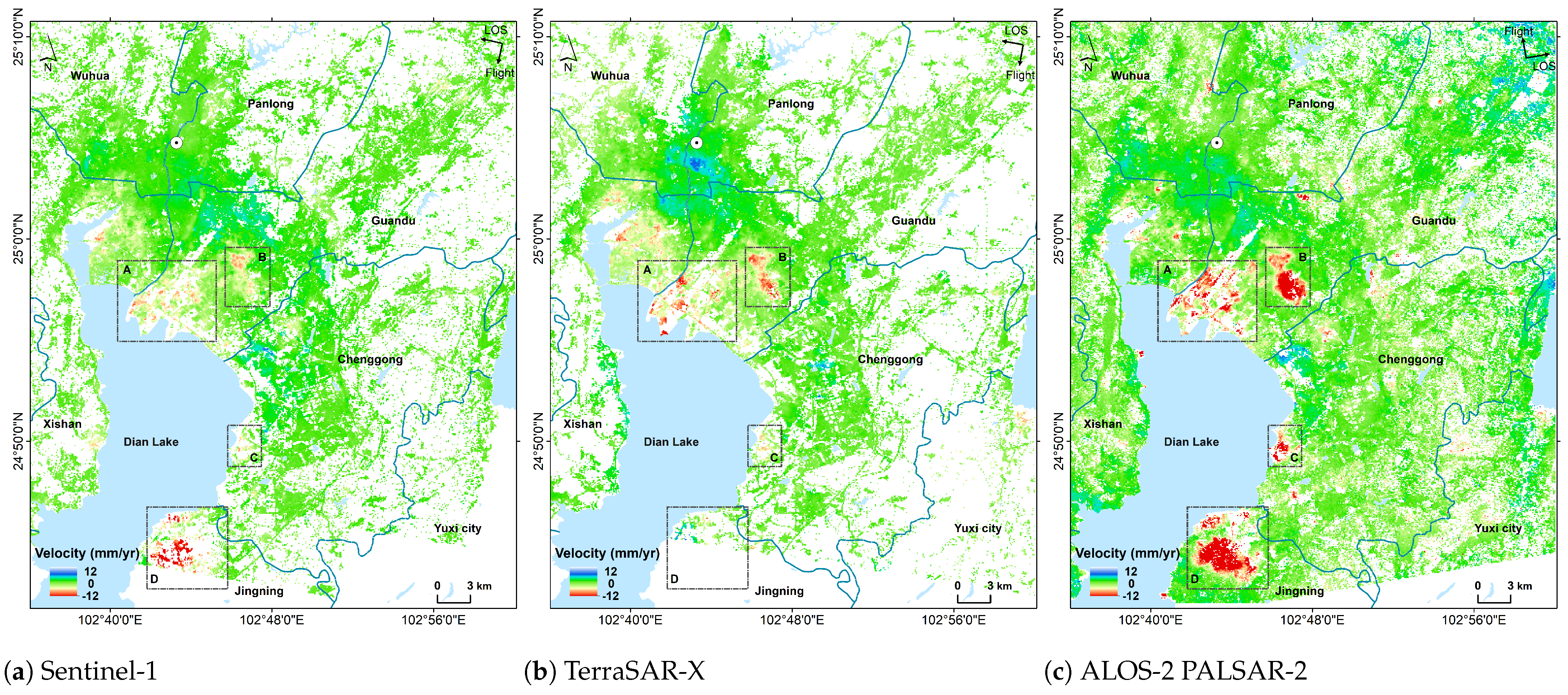
The PSI processing was performed using Sentinel-1, TerraSAR-X, and PALSAR-2 images, as detailed in
Section 3.1. The estimated line-of-sight (LOS) deformation linear velocity maps over the KMC area are depicted in
Figure 3. Negative values indicate displacement moving away from the satellite sensor, whereas positive values suggest deformation moving towards it. The estimated velocities ranging from −12 to 12 mm/yr are color-coded. It is important to note that a color bar spanning from −12 to 12 is utilized to emphasize the relatively smaller velocity values. Consequently, velocity values exceeding 12 are also color-coded, appearing as red or blue. The reference point, selected based on historical deformation data [
43,
44,
45] from the study area, is represented by a white circle in the resulting figures.
Upon examining
Figure 3, it is clear that all three data stacks detect similar deformation patterns. Generally, most downtown areas in KMC are stable, ranging from −3 to 3 mm/yr. Considering the potential errors in velocity estimation, velocity values within the range of −3 to 3 are considered as stable. However,
Figure 3 also shows four localized areas of abnormal deformation. Zones A, C, and D are located along Dianchi Lake. Zones A and B are within the Guandu district, C is in the Chenggong district, and D is in the Jingning district. Both Sentinel-1 and PALSAR-2 detected these deformation zones. Note that the TerraSAR-X data do not cover Zone D. A slight upward deformation was detected where Wuhua District and Panlong District intersect; this is the earliest urbanized area in Kunming, although the magnitude of upward deformation is minimal.
In this study, the total number and mean density (unit: PSs/km2) of PS points detected in the KMC area are 2,610,310 and 949 for Sentinel-1, 5,022,728 and 2283 for TerraSAR-X, and 3,592,430 and 1306 for PALSAR-2.The density of points mainly depends on the resolution of the image, so the point density of TerraSAR-X is the highest, followed by PALSAR-2, and Sentinel-1 is the lowest. The long wavelength of PALSAR-2 data helps maintain coherence, increasing the point density. It is obvious that, in regions with more significant deformations, ALOS data can extract the deformation results of the entire abnormal deformation area more completely.
The datasets were gathered beginning in 2017. Sentinel-1 observations extended until December 2022, PALSAR-2 until January 2022, whereas TerraSAR-X observations reached August 2019. If the deformation was primarily within a specific timeframe, a longer duration could smooth the estimation of the linear rate, resulting in a smaller overall rate as calculated by Sentinel-1. The variation in incidence angles results in identical vertical deformations appearing differently in the LOS direction. In these cases, the average incidence angle for TerraSAR-X is 31 degrees, for PALSAR-2 is 35 degrees, and for Sentinel-1 is 40 degrees. This suggests that S1 has the smallest sensitivity to vertical deformation. Additionally, with its longer wavelength, PALSAR-2 data tend to detect a more noticeable deformation gradients. The three datasets differ in ascending and descending orbits, incident angle differences, wavelength, and observation periods. However, the deformation distribution among them is comparable. This similarity suggests that vertical deformation primarily drives the entire area, and the evolution of deformation generally aligns with linear deformation.
This study involves working with three SAR datasets, each offering varying temporal and spatial resolutions. These allow us to generate three-dimensional deformations from the datasets, based on a uniform sampling grid and assuming linear velocity. Despite the significant research conducted on this topic [
46,
47], this study does not include three-dimensional deformation processing. This is due to two main reasons: First, deformation results based on a sampling grid are not suitable for heterogeneous urban scenes. The focus is on the temporal deformation characteristics of point targets. Second, LOS deformation analysis suffices for exploring the spatial distribution characteristics of deformations. Therefore, LOS deformations were analyzed in this study.
5. Discussion
This section provides the discussion on the noticeable deformation and possible causes. After examining the spatial pattern of deformation velocities and their associated factors, the focus will next be on the time series features of deformation. The proposed unsupervised learning analysis method was applied to classify the deformation series. This method emphasizes the kinematic characteristics of the PS and interprets the spatiotemporal deformation distribution in the study area. The logic behind the classification and their effectiveness in interpreting InSAR deformation signals are also discussed in this section. Finally, three indicators are introduced to explore the feasibility of the proposed unsupervised approach for classifying the InSAR deformation series.
5.1. Urban Construction and Abnormal Deformation Zone
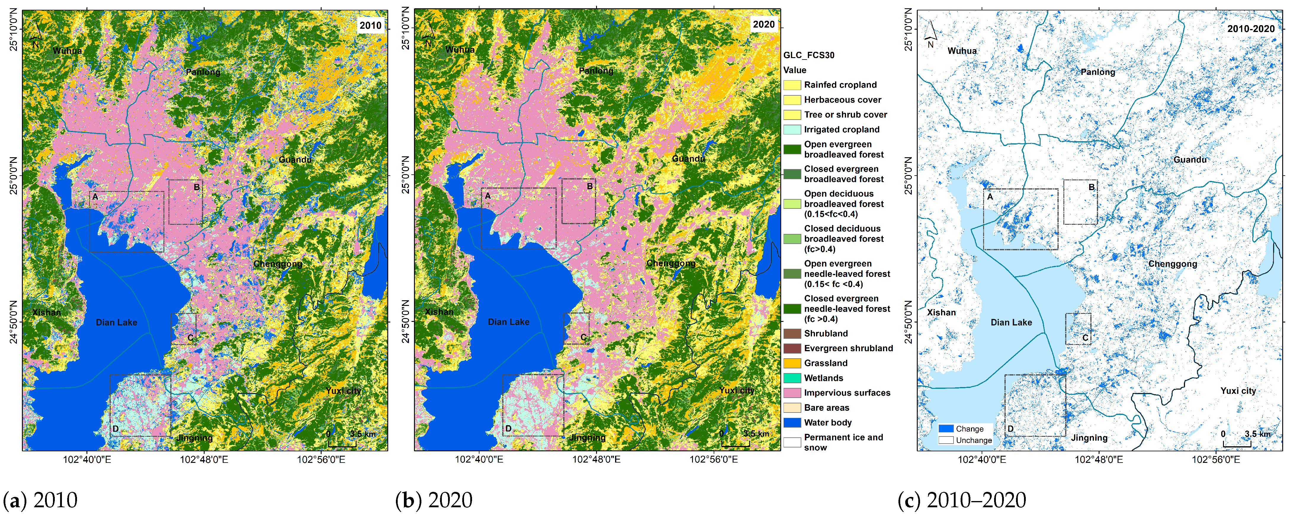
For interpreting the areas with abnormal deformation, the fine landcover classification product GLC_FCS30 [
48] of the research area was collected from 2010 and 2020. This product uses Landsat satellite data (Landsat TM, ETM+, and OLI) and the Google Earth Engine cloud computing platform to deliver a global 30 m landcover classification product with 29 categories.
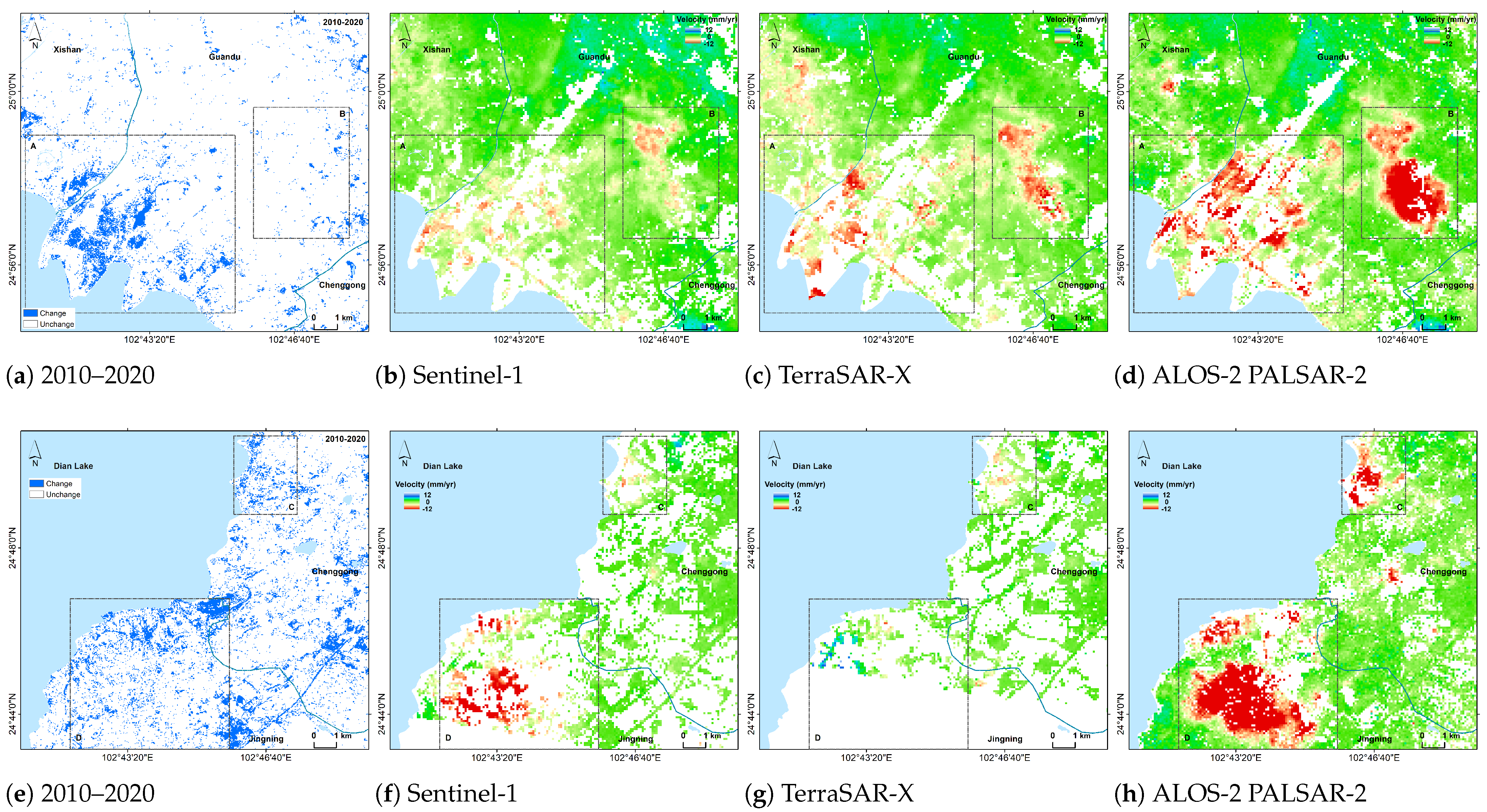
Figure 4 displays the fine classification maps of GLC_FCS30 in the KMC area for 2010 and 2020. The binary change map in
Figure 4c is generated by comparing whether the surface cover category in the same pixel has changed between different years. Here, a value of 1 indicates no change, whereas a value of 0 indicates a change.
To better understand the deformations identified on the velocity map in
Figure 3 for regions A, C, and D, detailed maps are provided in
Figure 5. These regions showed an increase in buildings, which corresponded to a decrease in water bodies. Located along the shores of Dianchi Lake, these changes could be linked to land reclamation projects that often involve dredging sediment from the lake bed or importing fill materials to create land. This process can cause ground settlement in areas with a soft soil foundation [
49]. Additionally, buildings constructed on such foundations may be prone to subsidence. In contrast, area B showed no correlation with changes in surface cover. Ground survey results suggest that the deformation in this area may be due to building instability, as evidenced by visible cracks and tilting. This area, comprising urban villages with numerous self-built houses, often lacks stringent building standards and effective management, which can result in tilting from additional floor construction [
44,
45]. In addition to construction-induced deformations, tectonic movements can also contribute to surface uplift and subsidence.
5.2. Unsupervised Learning InSAR Deformation Kinematic Characteristics
Five types of deformation kinematic characteristics were identified from Sentinel-1, TerraSAR-X, and PALSAR-2 in the InSAR deformation series. This was done using the method described in
Section 3.2, which involves PCA decomposition and unsupervised clustering. The spatial distribution of the clustering results are displayed in
Figure 6,
Figure 7 and
Figure 8. The number of clusters can be determined by analyzing clustering metrics. Here, the number of clusters was set to 5.
Figure 6a,
Figure 7a and
Figure 8a are color-coded by the classified group number, where each color signifies a different cluster type.
Figure 6b,
Figure 7b and
Figure 8b are the shadow line graphs plotted with the average and standard deviation of all InSAR deformation series in each cluster.
Figure 6c,
Figure 7c and
Figure 8c are the violin plots of the velocity distribution for corresponding clusters of PS points.
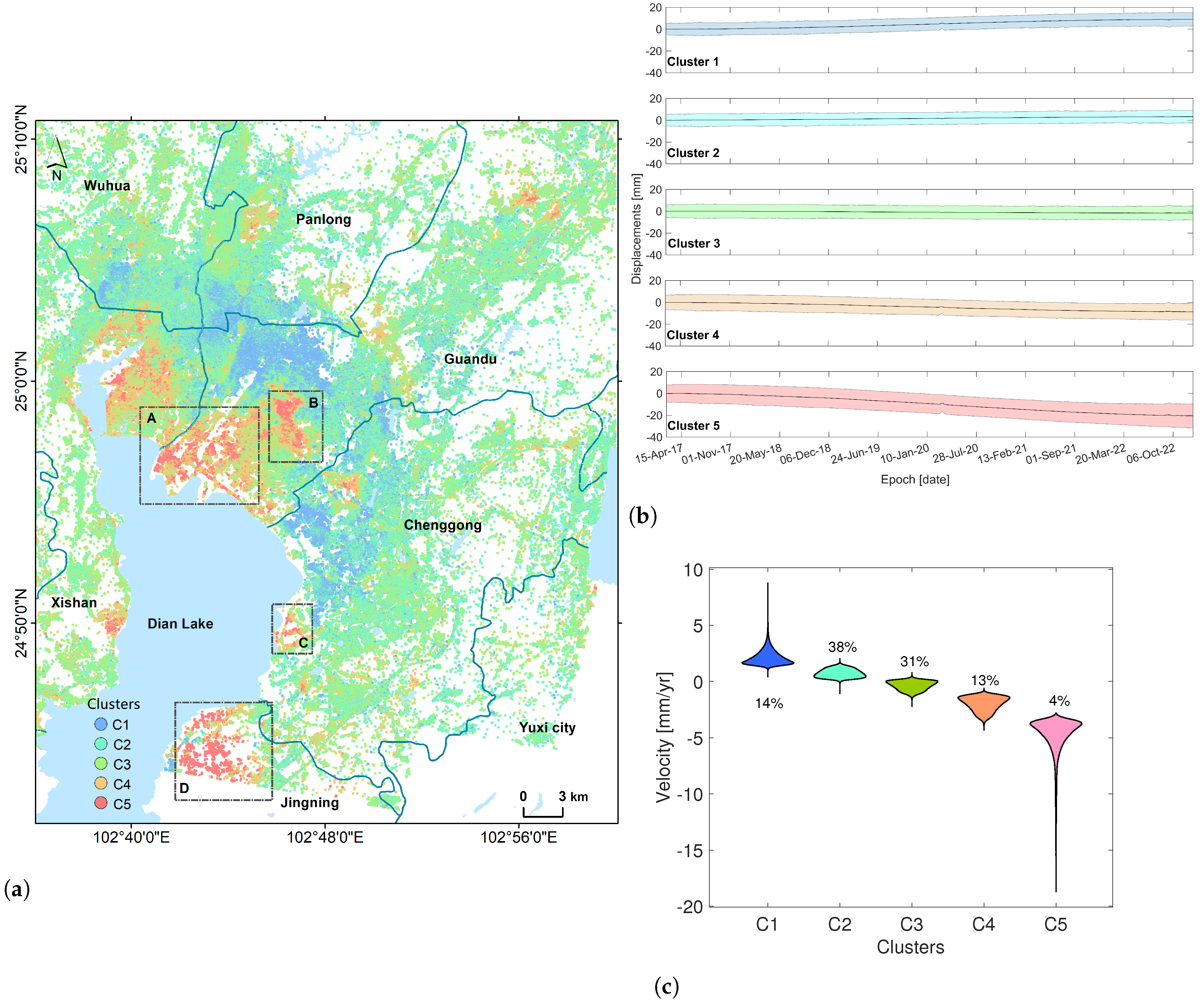
In
Figure 6, the unsupervised learning method has divided the time series deformation from Sentinel-1 data into five types: upward, slight upward, stable, slight downward, and obvious downward. The results in
Figure 6 closely resemble the velocity map in
Figure 3. However,
Figure 6 also explains the evolutionary characteristics of the low-velocity PS points. In clusters 2, 3, and 4, the velocity values are minor and similar, making it difficult to differentiate them. These three types comprise 82% of the total. In the analysis of deformation velocities, these points are often overlooked due to their relatively small rate values. Because these values are very close, they tend to be considered as the same type of deformation. However, in reality, these points exhibit different temporal evolution characteristics. In fact, 51% of the points actually show a slight upward or downward trend. While the value of deformation velocity might be small, it can gradually accumulate over time, potentially resulting in significant changes. Although cluster 5, marked in red, is noticeable, it only comprises 4% of the data. Cluster 5 frequently appears at the center of the deformation area, surrounded by cluster 4. Similarly, the regions marked as cluster 1 are surrounded by the slight upward labeled cluster 2. Such a distribution is also very reasonable.
Differences in velocities across the five categories are demonstrated upon observing and comparing
Figure 6b and
Figure 1c. The velocities of clusters 2 and 3 approximate 0, while the mean velocity of cluster 1 is slightly above 0 but less than 5, with some points exceeding 5. The average velocity of cluster 4 falls between −5 and 0, and the mean velocity of cluster 5 is above −5, but numerous points fall below −5.
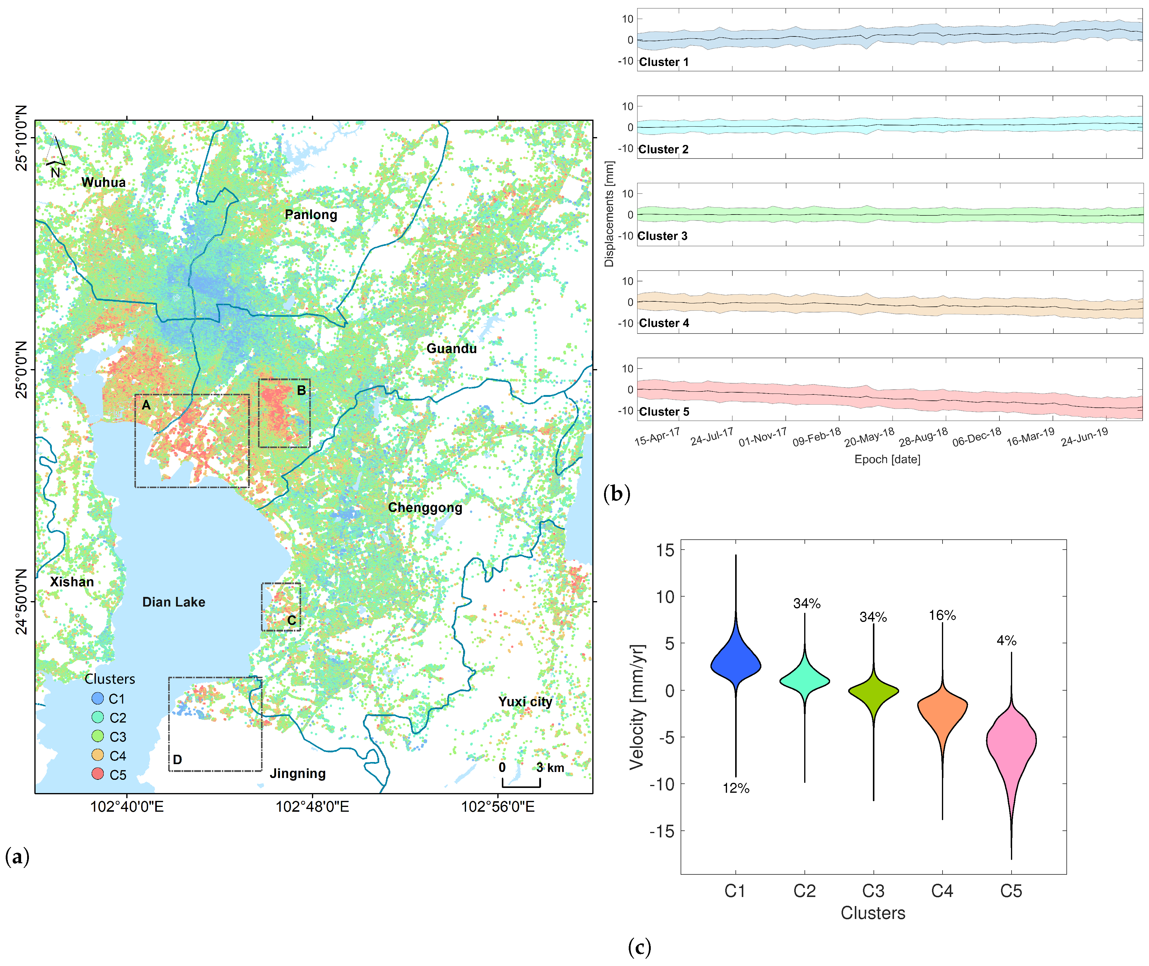
Figure 7 and
Figure 8 show the time series classification results of unsupervised learning for TerraSAR-X and PALSAR-2. Despite both utilizing unsupervised learning, a method without a sample set where classification relies on the inherent features of the datasets, the five categories provided by the three datasets are closely aligned. These categories denote upward, slight upward, stability, slight downward, and significant downward.
Table 2 outlines the proportions of these five categories derived from the three data types, demonstrating that the proportions are also closely matched.
When comparing
Figure 6 and
Figure 7, it is clear that the spatial distribution similarity of the TerraSAR-X and Sentinel-1 clustering results is high. However, the TerraSAR-X shows a smaller deformation magnitude ranging between −10 and 10 mm. In contrast, Sentinel-1 ranges between −40 and 20 mm. This likely concerns the differing detection capabilities of various band SAR data and observation geometry. Moreover, minimal mean velocity differences are observed among the TerraSAR-X clustering results. This suggests that, for results like TerraSAR-X, which detect smaller deformation magnitudes, it is challenging to differentiate between various types of deformation based solely on the velocities. In other words, the kinematic features are significant.
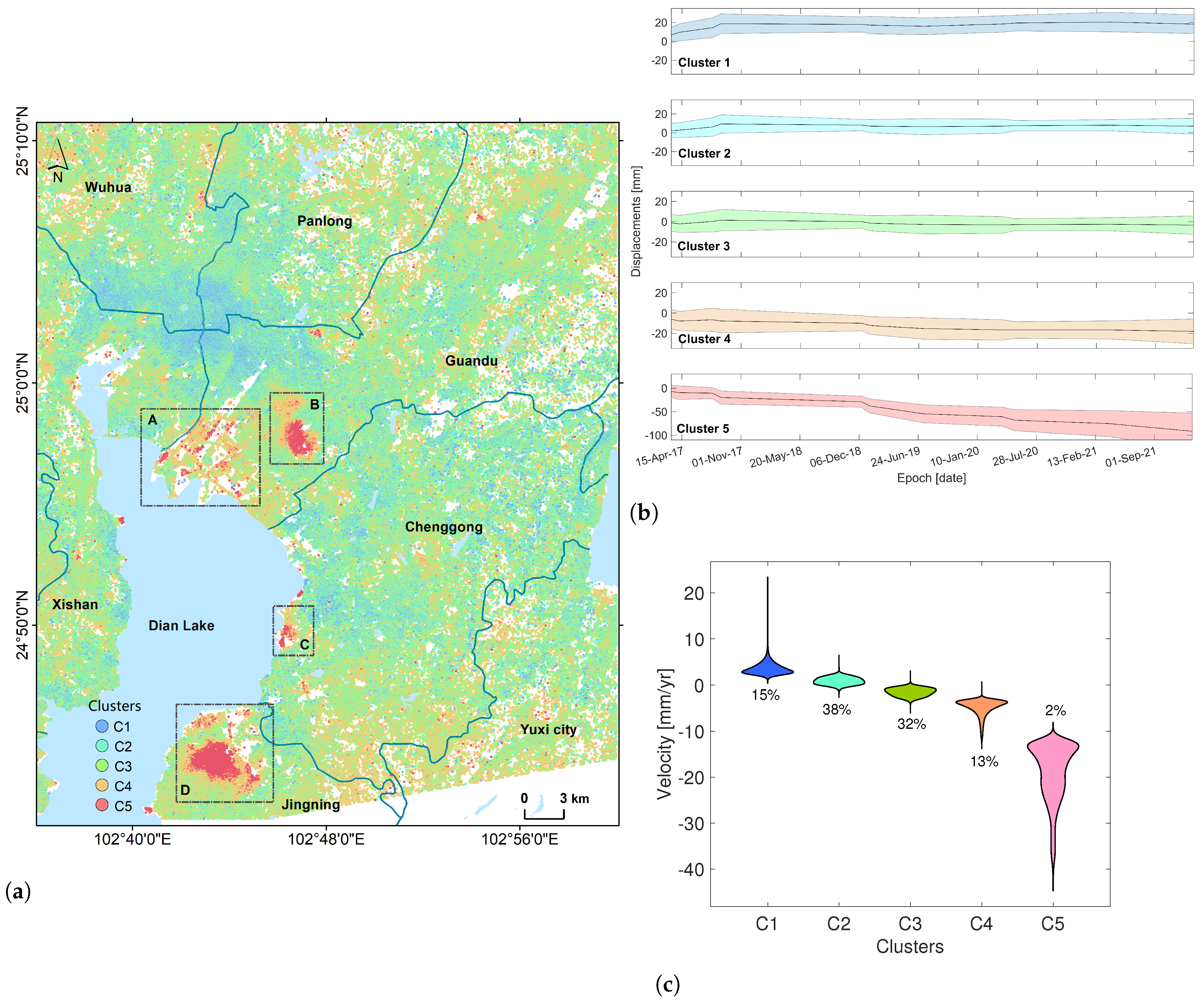
A high similarity in clustering results can be observed when comparing
Figure 8 with
Figure 6 and
Figure 7. It is interesting that, in areas where no PS points are detected in TerraSAR-X and Sentinel-1 data, they are prominently clustered in clusters 4 and 5 of the PALSAR-2 results. This suggests that PALSAR-2, with its long wavelength, can maintain coherence more effectively, or it might be due to the magnitude of deformation. Examining
Figure 8b, it is clear that the dispersion within the PALSAR-2 cluster is greater than that of TerraSAR-X and Sentinel-1. This may be due to fewer observation epochs in the PALSAR data. Furthermore, the deformation magnitude of cluster 5 in the PALSAR-2 results, ranging from −100 to 0 mm, is the largest, whereas cluster 4 aligns more closely with cluster 5 of Sentinel-1.
In conclusion, even though there are differences in wavelength, resolution, and observation time among the three datasets used (Sentinel-1, TerraSAR-X, and PALSAR-2), they deliver approximate results of unsupervised clustering based on time-series features within the study area. This approach can uncover more about the distinctions between PS points with minor velocities. As the InSAR deformation estimation result is a relative measure, delving into its time-series evolution rules could be a more appropriate strategy.
5.3. The Feasibility of PCA of InSAR Deformation Interpretation
This study presents an unsupervised learning method that combines PCA decomposition with k-means clustering for kinematic feature detection. This approach raises a question—is PCA decomposition essential? Can the original InSAR deformation series be used for clustering directly? This is explored from two perspectives: the role of PCA in time series deformation decomposition and the evaluation of the final clustering results.
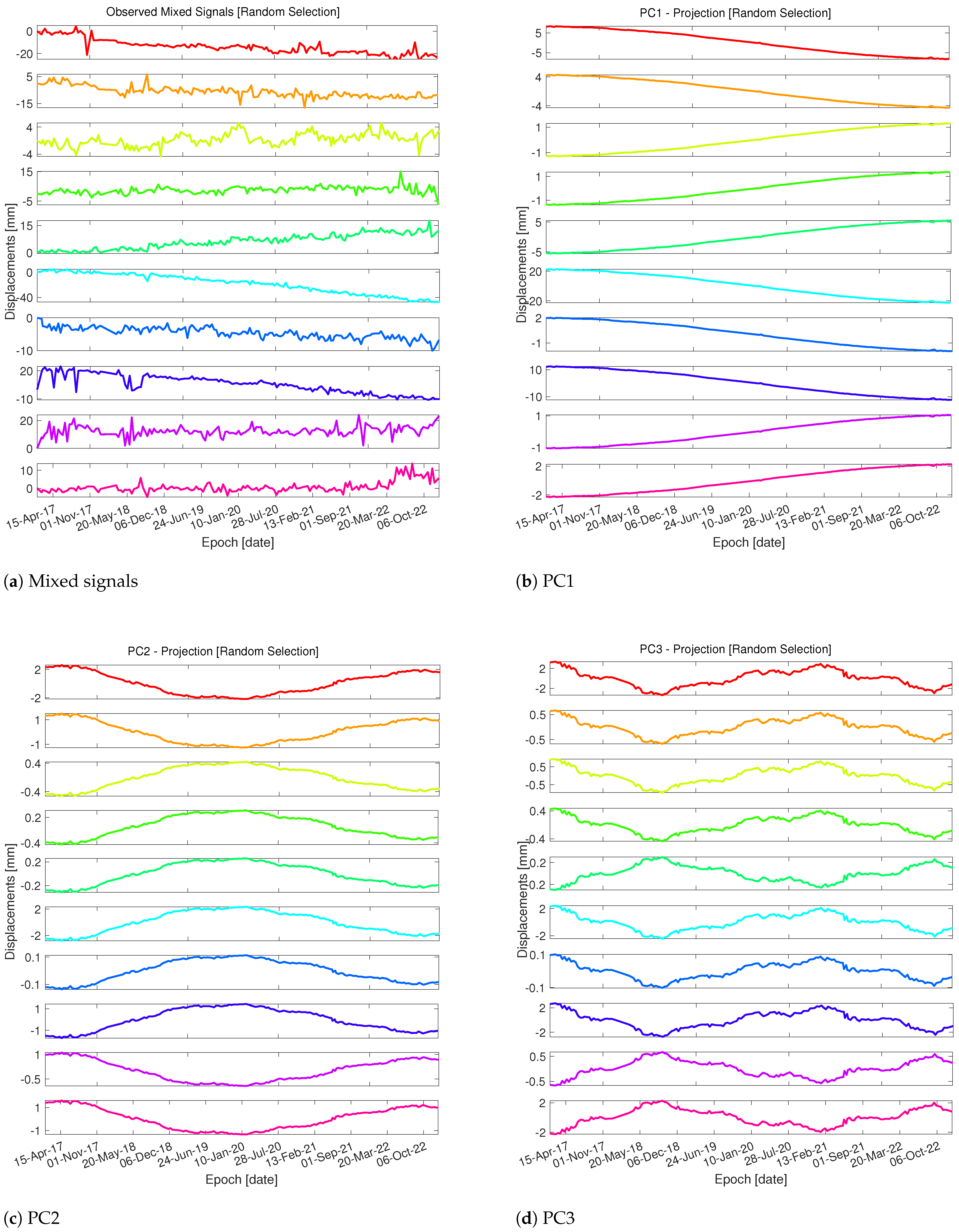
Ten time series deformations were randomly selected from the S1 data, and the results of their PCA decomposition are displayed in
Figure 9. First, in the decomposition of S1 data, PC1 is the trend term of the polynomial, PC2 is the sinusoidal contribution of the long time period, and PC3 is the sinusoidal contribution of the short time period. When observing the mixed deformation signals in
Figure 8a, due to the presence of noise, it is difficult to distinguish many points by relying on manual interpretation. However, by utilizing the PC1 component of the PCA decomposition, the trend of each PS point can be quickly assessed.
The 10 sequences in
Figure 9 are labeled from top to bottom as 1 through 10. Sequences 1, 2, 5, 6, 7, and 8 have clear trends that are easily identifiable as categories of upward and downward. For sequence 3, the range of its deformation value is small, making it difficult to categorize, even for experts. When using a sample-based deep learning recognition method, such deformation sequences are often classified as stable deformation points. This manual bias under noise conditions can lead to errors in supervised learning. However, after applying PCA decomposition, its subtle trends can be identified, making it more suitable for manual or machine learning. Sequences 4 and 9 also pose difficulties for manual identification, as they resemble random fluctuation signals. Thus, PCA has established a projection space that makes these sequences more comparable on a projection vector. This aids both manual and machine learning in better recognizing the sequence features.
Table 3 presents the results of three evaluation indicators as outlined in
Section 3.2. It also calculates the indicators based on the original InSAR deformation sequence and PC1. According to
Section 3.2, smaller indicators denote less discrepancy within the cluster and greater divergence among clusters, indicating a better overall clustering result. Generally, TerraSAR-X demonstrates the best clustering result, followed by Sentinel-1 and then PALSAR-2. This ranking could be attributed to the smaller magnitude of TerraSAR-X deformation data and the longer time series of Sentinel-1. Additionally, clustering based on PC1 is significantly better than that based on the original sequence, suggesting that PCA decomposition improves the distinction between sequences. The WB indicator based on SSW and SSB shows a particularly noticeable improvement.
The clustering indicators improve notably by using PCA decomposition. PCA decomposition improves the ability to identify distinct types within the time series. However, it is vital to realize the limitations associated with this method. The utilization of PCA decomposition specifically involved selecting PC1, which captures the maximum variation present in the data. Although this choice effectively summarizes the overall characteristics of the data, it may overlook certain deviations in sequence features. For example, in the experimental area, PC1 predominantly reflects a trend-oriented pattern resembling a linear polynomial. As a result, it fails to detect certain dynamic features such as step changes, acceleration, or seasonal variations during the clustering process. Despite these limitations, the proposed approach provides a valuable method for conducting large-scale time series deformation characteristics inspection.
6. Conclusions
Time series InSAR analysis is a powerful technique for monitoring surface deformation. With abundant SAR data and well-developed data processing techniques, deformation signals can be derived in areas of interest. However, interpreting these signals obtained through InSAR technology poses a challenge. Using the time series InSAR technique, velocities are calculated and time series deformation sequences are generated for millions of PS points. Deformation velocities offer a rapid overview of the severity of deformation, whereas time series deformation provides insights into its evolution. However, examining the deformation sequences for each point can be labor-intensive. As a result, only a few PS points in regions exhibiting significant deformation velocities are often concentrated on. Consequently, the InSAR deformation information may not be fully exploited, overlooking the time series deformation characteristics of the entire study area.
This study presents an unsupervised learning method for exploring time series deformation characteristics. It uses the signal decomposition principle of PCA to extract the main components from the InSAR deformation signal, emphasizing the dominant motion trend of the deformation sequence. Furthermore, unsupervised clustering is performed on the decomposed signals to group points with similar kinematic characteristics. Through this process, a spatio–temporal representation of deformation has been achieved in the study area.
The downtown area of Kunming City, Yunnan, was selected as the study area and datasets were gathered in C-, X-, and L-bands from Sentinel-1, TerraSAR-X, and ALOS-2 PALSAR-2 acquired from 2017 to 2022. This area was chosen due to the extensive knowledge and data from long-term research, and the proposed method has universal applicability across regions. Time-series InSAR technology was used to create deformation velocity maps of the area. The three datasets exhibited high similarity in their generated InSAR deformation velocity maps. Differences in deformation estimates were further analyzed from the viewpoints of point density, wavelength, imaging geometry, and data acquisition period.
When implementing the unsupervised learning approach, the three datasets showed consistency in the spatial pattern of clustering results. Five types of deformation characteristics were identified in the study area: upward, slight upward, stability, slight downward, and downward. The proportions of these five deformation types are also very close across the three datasets, ranging from 12% to 14%, 34% to 38%, 31% to 34%, 13% to 16%, and 2% to 4%, respectively. The proportion of PS points with relatively small deformation velocities is about 80%. However, in reality, only around 30% are relatively stable, whereas the remaining 50% of PS points, although exhibiting small values of velocities, still demonstrate a trend of movement.
Notably, compared to the analysis solely relying on InSAR deformation velocities, the suggested method can better highlight the kinematic characteristics of each PS point, particularly those with relatively small values of deformation velocities, which accounted for more than 50% of the total PS points. These deformation characteristics are often overlooked in conventional InSAR result analysis. Additionally, the efficiency of PCA in decomposing InSAR time series deformations was assessed using cluster evaluation metrics. PCA decomposition can simplify the differentiation of InSAR deformation sequences, thereby improving the efficiency of clustering. However, as pointed out in the discussion, focusing solely on the analysis of the dominant component may overlook some time-series abrupt signals. This limitation could serve as a promising topic for future research and exploration.


