Crop Canopy Nitrogen Estimation from Mixed Pixels in Agricultural Lands Using Imaging Spectroscopy

Abstract

Accurate retrieval of canopy nutrient content has been made possible using visible-to-shortwave infrared (VSWIR) imaging spectroscopy. While this strategy has often been tested on closed green plant canopies, little is known about how nutrient content estimates perform when applied to pixels not dominated by photosynthetic vegetation (PV). In such cases, contributions of bare soil (BS) and non-photosynthetic vegetation (NPV), may significantly and nonlinearly reduce the spectral features relied upon for nutrient content retrieval. We attempted to define the loss of prediction accuracy under reduced PV fractional cover levels. To do so, we utilized VSWIR imaging spectroscopy data from the Global Airborne Observatory (GAO) and a large collection of lab-calibrated field samples of nitrogen (N) content collected across numerous crop species grown in several farming regions of the United States. Fractional cover values of PV, NPV, and BS were estimated from the GAO data using the Automated Monte Carlo Unmixing algorithm (AutoMCU). Errors in prediction from a partial least squares N model applied to the spectral data were examined in relation to the fractional cover of the unmixed components. We found that the most important factor in the accuracy of the partial least squares regression (PLSR) model is the fraction of photosynthetic vegetation (PV) cover, with pixels greater than 60% cover performing at the optimal level, where the coefficient of determination ($R^2$) peaks to 0.66 for PV fractions of more than 60% and bare soil (BS) fractions of less than 20%. Our findings guide future spaceborne imaging spectroscopy missions as applied to agricultural cropland N monitoring.

1. Introduction

Imaging spectroscopy has emerged as a powerful tool to monitor and characterize Earth’s surface, providing unprecedented spectral information about the properties of land cover components. Among the many applications of imaging spectroscopy, the quantification of photosynthetic vegetation (PV); non-photosynthetic vegetation (NPV), i.e., the vegetation that cannot perform photosynthetic function, e.g., dead biomass; and bare soil (BS) fractions are of particular importance [1,2,3], particularly for studies on carbon storage [4] and tillage management [5], hydrology (through controlling mass and energy balance), uptake of nutrients, and soil wind erosion in croplands [6,7]. However, quantifying these fractions from imaging spectroscopy is a challenging task, as it requires separating the mixed spectral signatures of different land cover components [8,9,10]. In previous studies, various unmixing methods have been developed to address this challenge, providing promising solutions for quantifying the fractions of PV, NPV, and BS from imaging spectroscopy [11], ranging from linear unmixing [3] to machine learning algorithms [12,13] to separate the mixed spectral signatures of different land cover components [14]. These methods have been applied to a wide range of applications, including vegetation monitoring [15], land cover change detection [16], and agricultural productivity mapping [17].

Precision agriculture aims to optimize crop production by tailoring management practices to the specific needs of individual plants or field areas. One key aspect of precision agriculture is the accurate estimation of nitrogen (N) content in crops, as it directly impacts crop growth and productivity [18]. Imaging spectroscopy has emerged as a valuable tool for the nondestructive and large-scale estimation of N content in crops [19,20]. However, the accuracy of these estimates is influenced by the presence of other components in the field of view, and consideration of the cover fractions of different land cover components, such as PV, NPV, and BS [21,22], is necessary. The PV, NPV, and BS fractions play a role in estimating the N crop canopy from imaging spectroscopy through their direct connection to plant tissue storage of N. PV is a primary source of chlorophyll, which correlates highly with the total stored nitrogen in a plant [23]. Several studies have been conducted to estimate nitrogen content in crops using imaging spectroscopy, for instance in our previous study [24], the reflectance data are used to train and develop a partial least squares regression (PLSR) model over the homogeneous green pixels, i.e., spectral filters are applied to exclude pixels with significant contributions of NPV and BS. Asner et al. [25] employed GAO visible-to-shortwave (VSWIR) infrared imaging spectroscopy and LiDAR to map the foliar traits (including N) of tropical forests in the Amazon. PLSR is employed in the mentioned study to quantitatively associate airborne VSWIR spectroscopy data with foliar traits assessed in the laboratory from field-collected samples. In another research, the PLSR model is used to investigate the capacity of field spectroscopy to predict seasonal changes in leaf functional traits across eight deciduous tree species in the UK [26]. It finds that while leaf spectroscopy can accurately estimate the seasonal variation in most traits, the accuracy of a single PLSR model varies among traits and species through the growing season. However, studies quantifying the effect of changes in fractional cover on this relationship are lacking in the literature to the best knowledge of the authors. This paper aims to investigate the impact of cover fractions on estimating N from imaging spectroscopy using a statistical model.

In this study, we sought to understand the impact of fractional cover on the retrieval of N content in agricultural landscapes using imaging spectroscopy. This was conducted as part of the research program for the Carbon Mapper Land and Ocean mission (https://carbonmapper.org/ (accessed on 24 May 2021)), which was designed to study and assess current methodologies in imaging spectroscopy for delivering comprehensive insights into land and ocean resources [27]. For this study, airborne imagery was collected concurrently with a series of field campaigns using the Global Airborne Observatory (GAO), which is equipped with advanced visible-to-shortwave infrared (VSWIR) technology. We used AutoMCU, an automated Monte Carlo Unmixing approach, to unmix the fractional cover of three target endmembers (here PV, NPV, and BS) within each pixel [3]. We used these estimated fractional cover values to assess the impact of these fractional cover estimates on the performance of models of plant N content derived from a model directly linking N content to the spectral reflectance of the pixel. In the current study, the obtained reflectance data are fed into the PLSR and AutoMCU models to retrieve N content and cover fraction, respectively. Then, the relation between the fractional cover over agricultural lands and estimated N content is investigated. While the methods of the lab measurement and PLSR model of plant N content are briefly discussed in this paper, more comprehensive details can be found in a companion paper [24]. Using these tools, we examined the impact of cover fraction variations on the accuracy of N estimation from the PLSR model. Our results contribute to a better understanding of the factors affecting the accuracy of N estimation in mixed pixels and provide insights into the development of more accurate models using imaging spectroscopy.

2. Methods

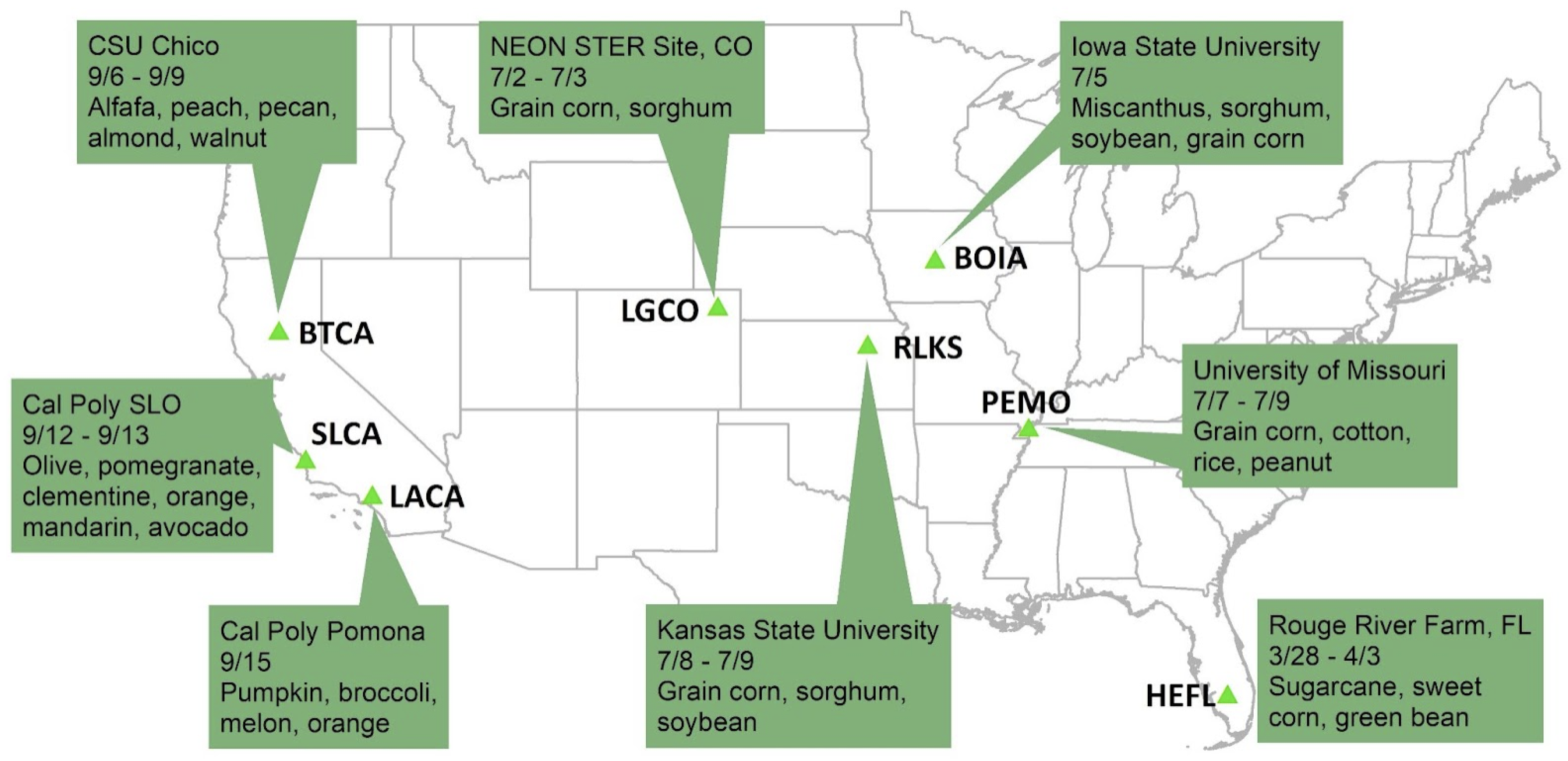
2.1. Field Campaigns to Collect Leaf Samples

To obtain leaf samples from various crops, we visited farms in six states within the USA: Florida (FL), California (CA), Colorado (CO), Iowa (IA), Kansas (KS), and Missouri (MO). Sampled species represented commodity crops such as corn, soybean, sorghum, miscanthus, green bean, alfalfa, cotton, vegetables, and orchard fruits. A complete list of the species collected at each site and their relative sample sizes can be found in

Table 1. List of sampled crops with the number of samplings from six states in the USA: California (CA), Florida (FL), Missouri (MO), Iowa (IA), Kansas (KS), Colorado (CO).

Crop	# Samples	State
Alfalfa	15	CA
Cotton	20	MO
Green Bean	16	FL
Grain corn	103	IA, KS, CO, FL, MO
Sweet corn	15	FL
Soybean	38	IA, KS
Sorghum	59	IA, KS, CO
Miscanthus	18	IA
Peanut	15	MO
Tree nuts:	45	CA
Walnut, Almond, Pecan	(3×15)
Fruit tree:	110	CA
Peach, Orange, Mandarin, Avocado, Olive, Pomegranate, Orange, Clementine	(15 sampling points for the first 7 crops and 5 sampling points for the last crop)
Vegetables:	15	CA
Pumpkin, Broccoli, Melon	(3×5)
Total	469	6

. Sampling efforts were concentrated in areas where crop conditions appeared uniform, with samples collected within a one-meter radius at each recorded point. Depending on the leaf size, we harvested up to twenty mature leaves from the sunlit upper canopy of each plant for each sampling location. Then, clipped foliage was immediately sealed in polyethylene bags and stored on ice in coolers to preserve moisture. For each species at every location, our protocol was to collect 15 samples from a single field, or a total of 20 samples across multiple fields when feasible. GPS readings were recorded at the sample locations using Arrow Gold RTK Global Navigation Satellite Systems receiver with an estimated horizontal positioning precision of ≤1 cm. The complete dataset comprised 469 individual foliage samples, representing 23 species collected from eight sites in six states. Foliage samples were processed within two hours of collection. The processing steps are explained comprehensively in [24]. The N concentration of each processed leaf sample was determined in the lab by flash combustion in a conventional elemental analyzer (PE 2400; PerkinElmer Inc., Waltham, MA, USA).

The location of the sampling points with the farm names and the dates when the leaves were collected is shown in Figure 1.

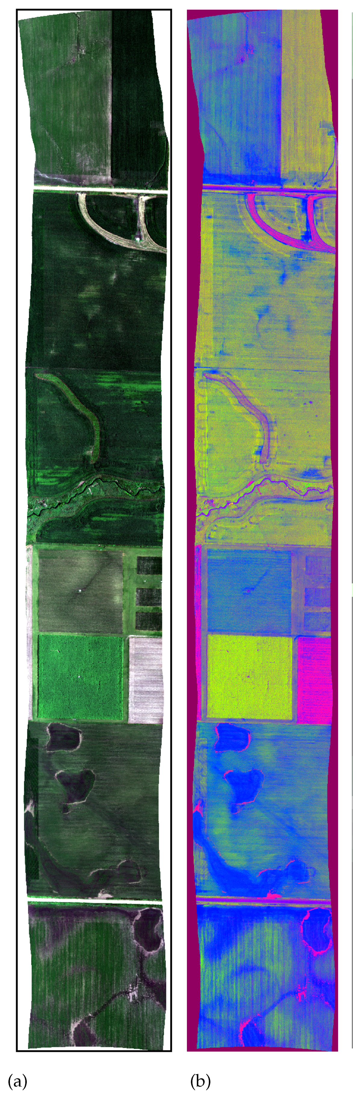
2.2. Airborne Imaging Spectroscopy

Within fewer than six days of the collection of field samples, the GAO collected imaging spectroscopy data in the VSWIR region of the spectrum. The dataset collected for this study contained 428 spectral channels with a sampling spectral resolution of 5 nm, covering the wavelength range between 350 nm and 2490 nm. The flights were conducted at a height of 600 m above the ground, which led to an average ground sampling distance of 0.6 m. In addition, LiDAR data were collected concurrently with the imaging spectroscopy data to assist in the ortho-georeferencing of the images, generating digital terrain and surface models. To obtain surface reflectance, the VSWIR data were first preprocessed into orthorectified radiance and then corrected for atmospheric interference using ACORN v6.0 (Atmospheric CORrection Now; AIG LLC; Boulder, CO [28]). The wavelength range with significant atmospheric interference was removed, resulting in three spectral regions spanning wavelengths from 420 to 1330, 1500 to 1775, and 2030 to 2445 nm [24].

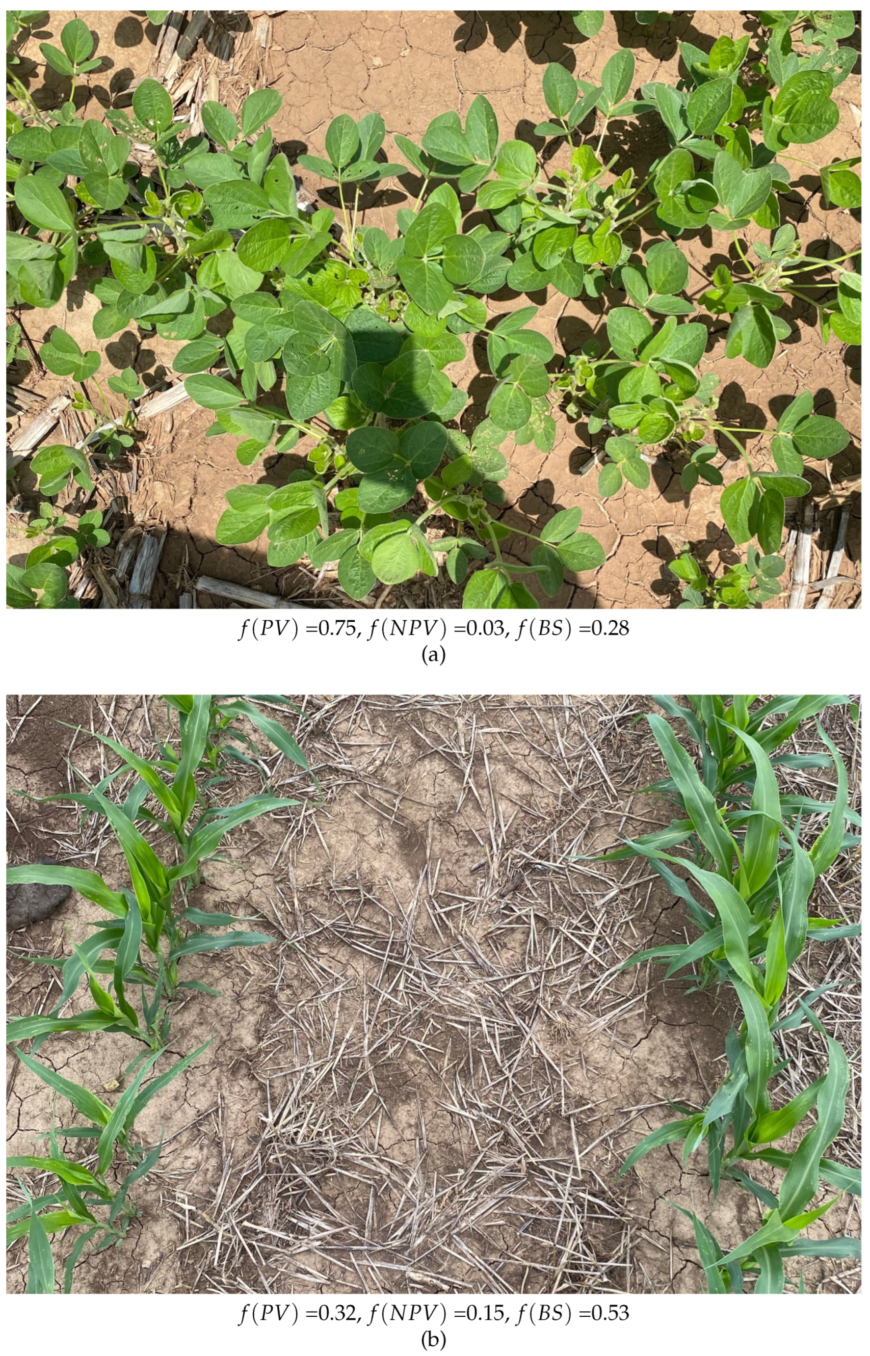
2.3. Quantifying Cover Fraction Using AutoMCU

Spectral Mixture Analysis (SMA) is a widely used unmixing method that decomposes a mixed pixel spectrum into a linear combination of multiple endmember spectra, representing pure materials such as vegetation or soil. SMA assumes that the spectrum of a mixed pixel can be modeled as a linear mixture of the spectra of its constituent materials, with the mixing coefficients representing the cover fractions of each endmember in the pixel [29]. This can be represented as in Equation (1), where $f_x$ is the fraction coefficient that should sum to nearly 1.0, $\rho {\left(\lambda \right)}_x$ are the input class example constituent spectra along wavelength $\lambda$, and $ϵ$ is an error term. SMA can be applied to both multispectral and hyperspectral data and has been used to quantify the cover fractions of PV, NPV, and BS [30,31].

$$\rho {\left(\lambda \right)}_{pixel}=f_{PV}\rho {\left(\lambda \right)}_{PV}+f_{NPV}\rho {\left(\lambda \right)}_{NPV}+f_{BS}\rho {\left(\lambda \right)}_{BS}+ϵ$$

(1)

Typically, photosynthetic vegetation (PV) effectively absorbs photons in the visible wavelengths, whereas non-photosynthetic vegetation (NPV) and bare soil have lower absorption rates. The red-edge slope, which is indicative of chlorophyll and structural differences, can differentiate between PV and NPV and bare soil [1,2]. Moreover, in the SWIR-2 wavelength range (2100–2400 nm), water effectively absorbs photons, leading to lower PV reflectance compared with NPV and bare soil [3]. Unlike PV, which efficiently absorbs SWIR wavelengths, dead, dry, or senescent vegetation (NPV) scatters photons throughout the SWIR range. The SWIR region (1300–2500 nm) is primarily dominated by water absorption and an increase in leaf water content results in decreased reflectance. Thus, the reflectance of PV in the SWIR region is lower than that of NPV [3]. Additionally, the unique absorption features of lignin and cellulose within this range allow for the identification of NPV and soil in the SWIR wavelength region. Understanding these absorption features is crucial for applying the AutoMCU algorithm in finding fractional coverage.

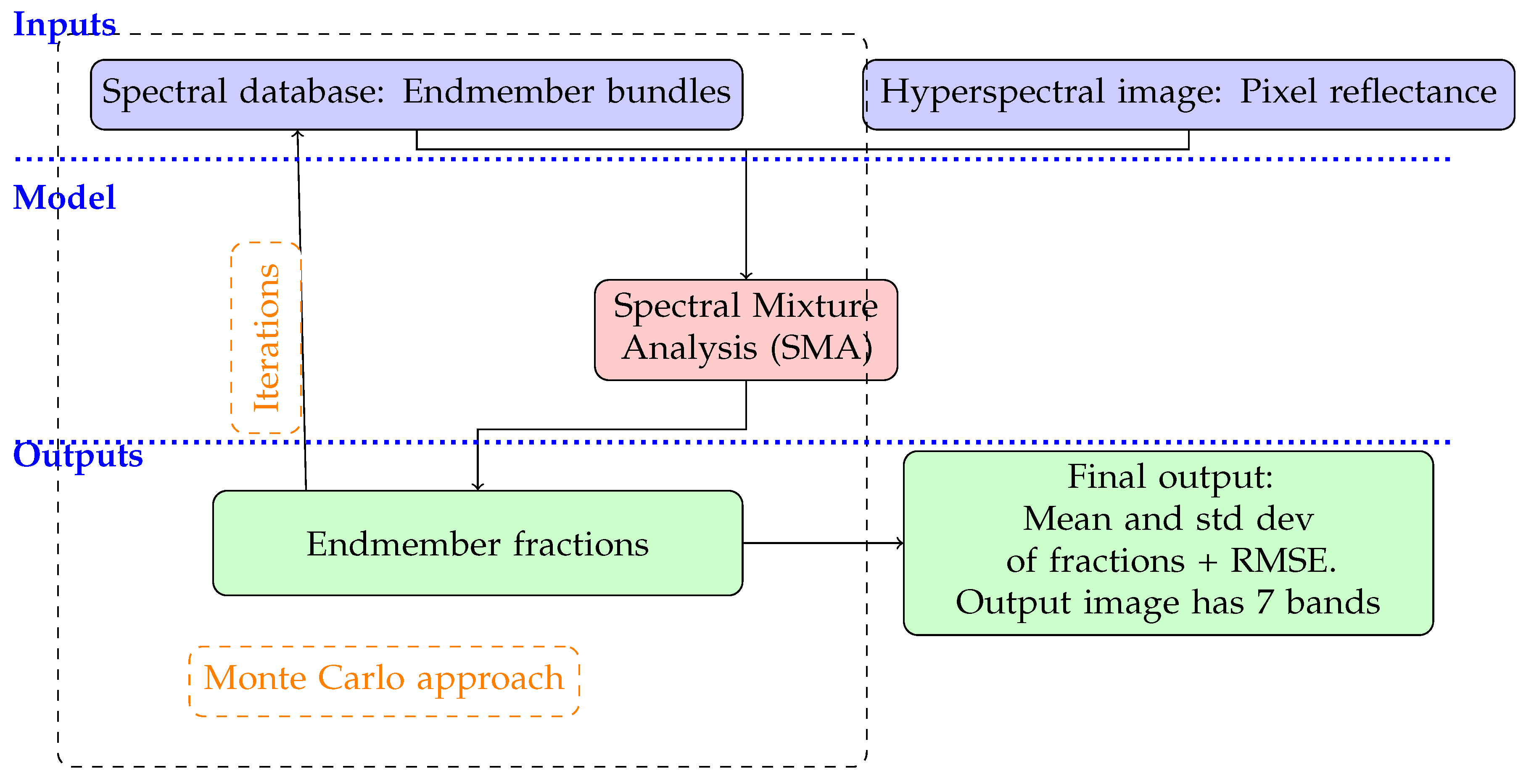
2.3.1. AutoMCU Description

The Automatic Monte Carlo spectral Unmixing model (AutoMCU) is based on SMA that was proposed by Asner and Heidebrecht [3], in which a large number of endmember combinations for each pixel is calculated by randomly selecting spectral data from a spectral library. Based on prior research conducted to develop AutoMCU by [2,3], it has been observed that when a sufficient number of endmember combinations are accessible, the fractional cover of different endmembers each exhibits a normal distribution. Thus, to obtain the final fractional cover for each pixel, the average value of each cover fraction across a large number of example endmember spectra can provide a reasonable estimate of the desired cover constituent. To achieve this, AutoMCU uses an iterative Monte Carlo resampling approach to quantify the fractional coverage of specified target constituents. For each of m user-specified iterations, the algorithm selects a new random combination of one endmember spectra from each of the endmember library bundles to unmix the image spectrum. Subsequently, endmember fraction means and standard deviations are computed across the m sets of fractions estimated from all iterations. The algorithm generates subpixel cover fraction values along with uncertainty estimates, which account for the variability in the endmember bundles. A schematic workflow of the AutoMCU algorithm is shown in Figure 2. The AutoMCU code used in this manuscript is accessible upon request to the corresponding author ([email protected]).

The AutoMCU capitalizes on two spectrum regions proved in previous studies [2,3] to strongly differentiate the spectral characteristics of PV, NPV, and BS, illustrated in Figure 3, which depicts the distinctions among the spectral characteristics of PV, NPV, and BS. The shaded region corresponds to the range of wavelengths employed by the AutoMCU algorithm in the present study for quantifying the fractions of each cover type within mixed pixels.

As explained above, the SWIR-2 (2100–2400 nm) region is dominated by foliar water absorption in PV spectra, whereas drier NPV vegetation allows the absorption features of organic compounds like cellulose and lignin to stand out at 2100 and 2300 nm. In contrast, BS spectra typically have a hydroxyl absorption feature at 2200 nm. The visible-to-NIR range (600–800 nm) contains the red edge feature of green vegetation. In general, reflectance decreases with increasing organic matter and/or water content in vegetation or soil. Due to the unique spectral shape of green vegetation in the red edge, this region provides good separation between PV from both NPV and BS [2].

To reduce the effects of brightness changes across an input image, some form of regularization is needed to ensure that the example spectra for each class can properly fit the observed spectra. Traditional brightness normalization methods, where spectra are divided by some measure of total brightness such as the vector norm, would destroy the linearity assumption of SMA. Instead, in AutoMCU, all spectra are “tied” to maintain this linearity. To tie the spectra, the reflectance value of the first entry in each fitting window (red edge, SWIR2) is subtracted from all reflectance values within that window (Figure 4). This zeroes out the first value of each window but standardizes the remaining spectra to stabilize PV retrievals across variations in biomass, canopy architecture, and biochemistry. After all the iterations are complete, the estimated fractions for each input image pixel are determined by computing the trimmed mean endmember fractions for this pixel across all iterations.

The cover fraction values obtained from AutoMCU are typically expected to fall within the range of [0, 1], representing the absence or presence of specific endmember fractions within a pixel. Because only a weak constraint is used to coerce the coefficients to sum to 1, an extra column of 1 values is added at the end of both fitting windows in both the endmember and observed spectra, and sums differing from 1 and negative cover coefficients occur. This is due to various factors including shading or discrepancies between observed spectra and the library dataset. These factors also introduce uncertainties that should be taken into account when interpreting the results and evaluating the accuracy of cover fraction estimation [32]. In this study, cover fraction values were truncated into the range [0, 1] and rescaled to sum to 1. Two measures of uncertainty were also saved: (1) the standard deviation (std dev) of the fractions across iterations, and (2) the $RMSE$ derived by comparing the model-estimated mixture spectra using the averaged coefficients against the observed spectrum for each input image pixel.

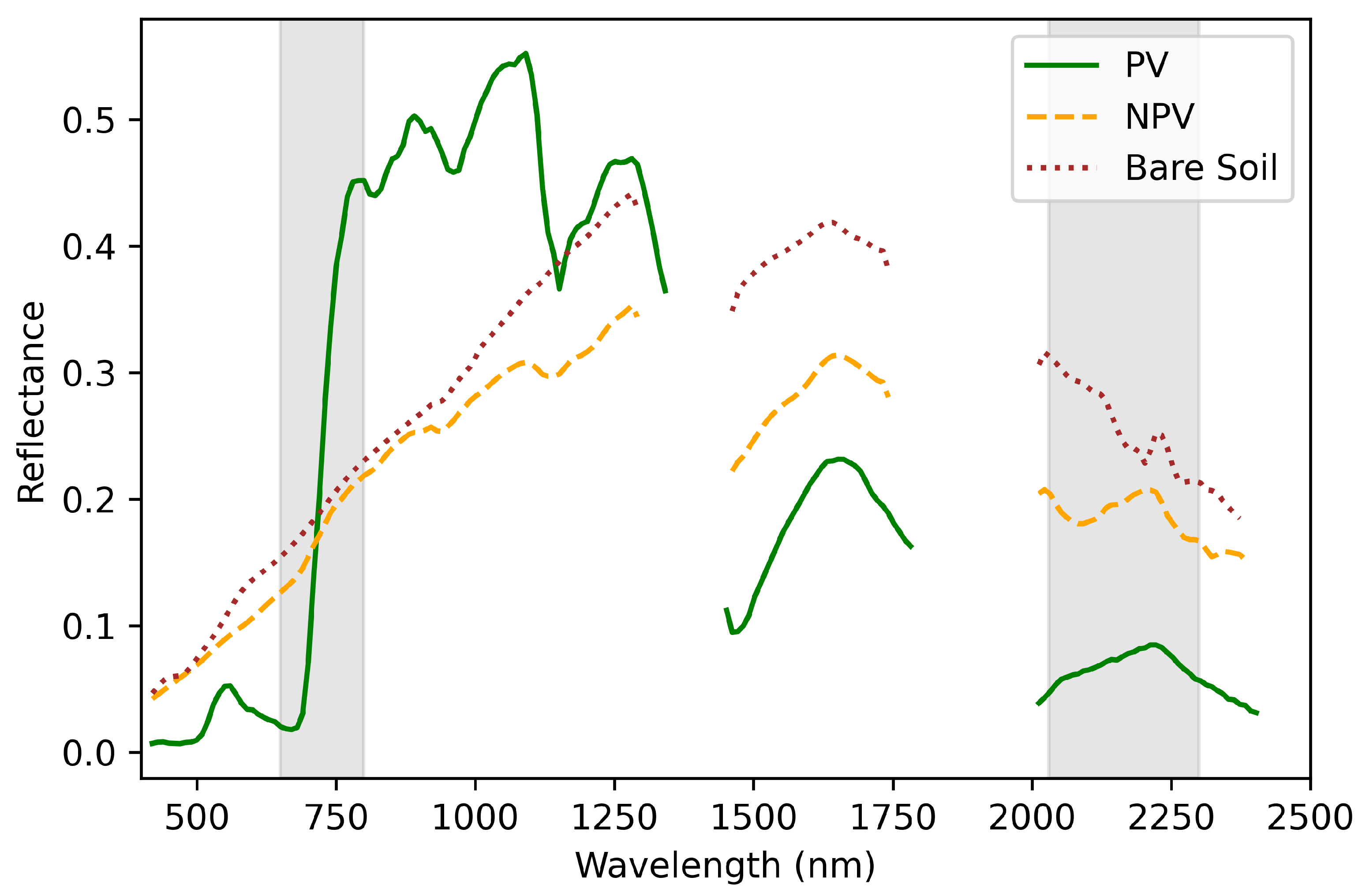
2.3.2. Spectral Library

Spectral libraries are an essential component of remote sensing analysis. A spectral library is a collection of spectra representing different materials, such as green vegetation, dead vegetation, soils, water bodies, and human-made objects. These libraries provide a reference for the comparison and identification of unknown spectra. In the context of cover fraction mapping and the scope of this research, spectral libraries for PV, NPV, and BS are particularly useful. These spectral libraries are typically derived from field or laboratory measurements of reflectance spectra.

There are several publicly available sources of spectral libraries that can be used for remote sensing analysis. One such source is the United States Geological Survey (USGS) Spectral Library [33], which contains spectra of minerals, rocks, soils, vegetation, and man-made materials. Another source is the ASTER Spectral Library [34], which contains reflectance spectra of minerals, rocks, soils, and vegetation. Additionally, the NASA Jet Propulsion Laboratory (JPL) Spectral Library contains laboratory measurements of a wide range of materials, including minerals, rocks, soils, vegetation, and man-made materials. These publicly available spectral libraries can be used to train and validate remote sensing algorithms and models, and to aid in the interpretation of remote sensing data. In this study, the spectral library from ECOSLib (https://speclib.jpl.nasa.gov (accessed on 2 February 2018)) [35] was used as the input for AutoMCU. ECOSpecLib includes data from three other libraries (John Hopkins University, JPL, and USGS; it is an update of the ASTER SLI 2.0 [34]).

2.4. Crop Nitrogen (N) Estimation

Partial least squares regression (PLSR) was used to link wet assay estimates of leaf N to imaging spectroscopy data collected by GAO [36]. PLSR is a linear regression technique for imaging spectroscopy that easily incorporates hundreds of bands of spectral information using a built-in data reduction akin to principal components analysis to eliminate the correlation between input variables [24,37]. This method has been widely employed in remote sensing applications to quantify plant functional traits [38,39,40]. Model reliability was addressed by utilizing two levels of iteration in the calibration–validation step. During each iteration, PLSR outcomes were evaluated using testing data and two performance statistics, the coefficient of determination ($R^2$) and Root Mean Square Error ($RMSE$), generated for both training and testing datasets. The final PLSR model was created by averaging the outcomes from all iterations. For a detailed description of the implementation of PLSR to these data, refer to our recent study [24]. In the current study, the spectral coefficients to fit on the dataset were retrieved for green pixels, based on NDVI filter $\ge 0.7$ [24]. The coefficients were then implemented through the PLSR model, which was fit to the spectral dataset over all sampled locations that include 469 pixels from aerial images. Additional details regarding the algorithm employed for N retrieval and the corresponding Python code can be found in the NitrogenRetrieval repository on our GitHub page, accessible at the following URL: https://github.com/CMLandOcean/NitrogenRetrieval [41] (accessed on 24 May 2021).

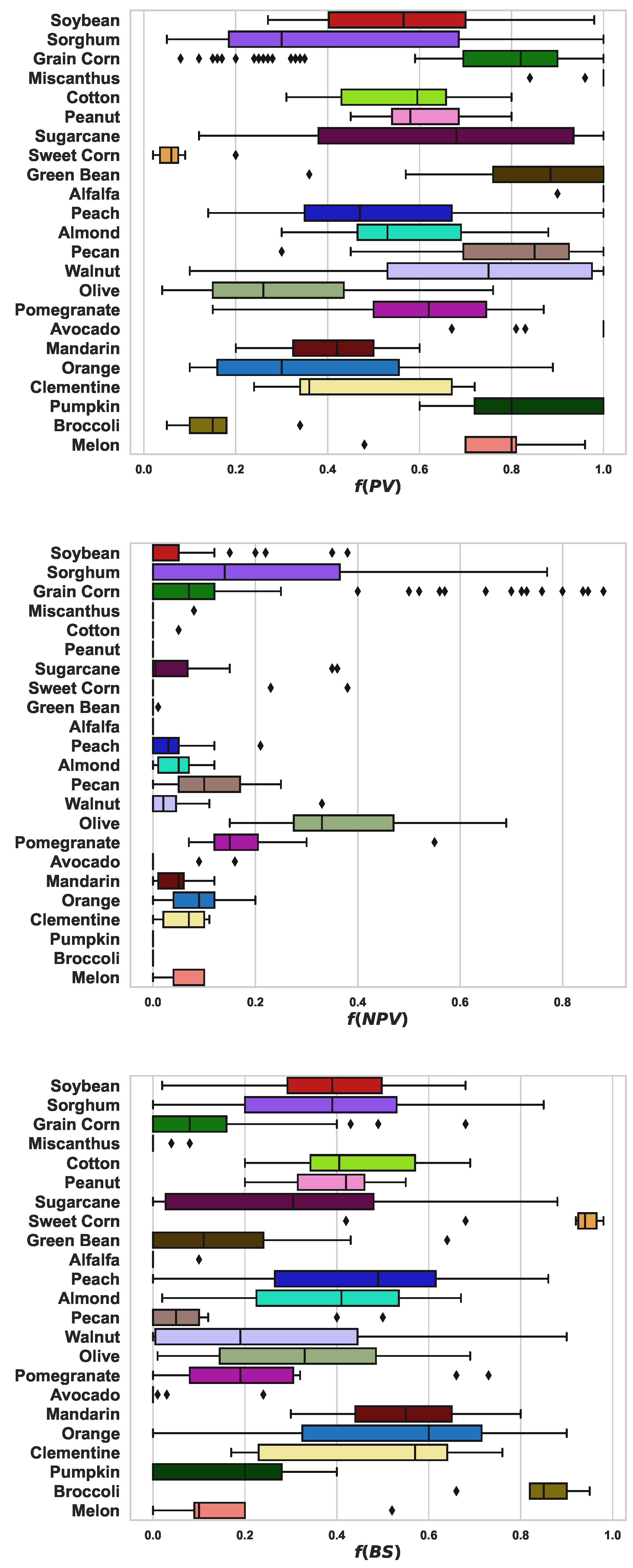
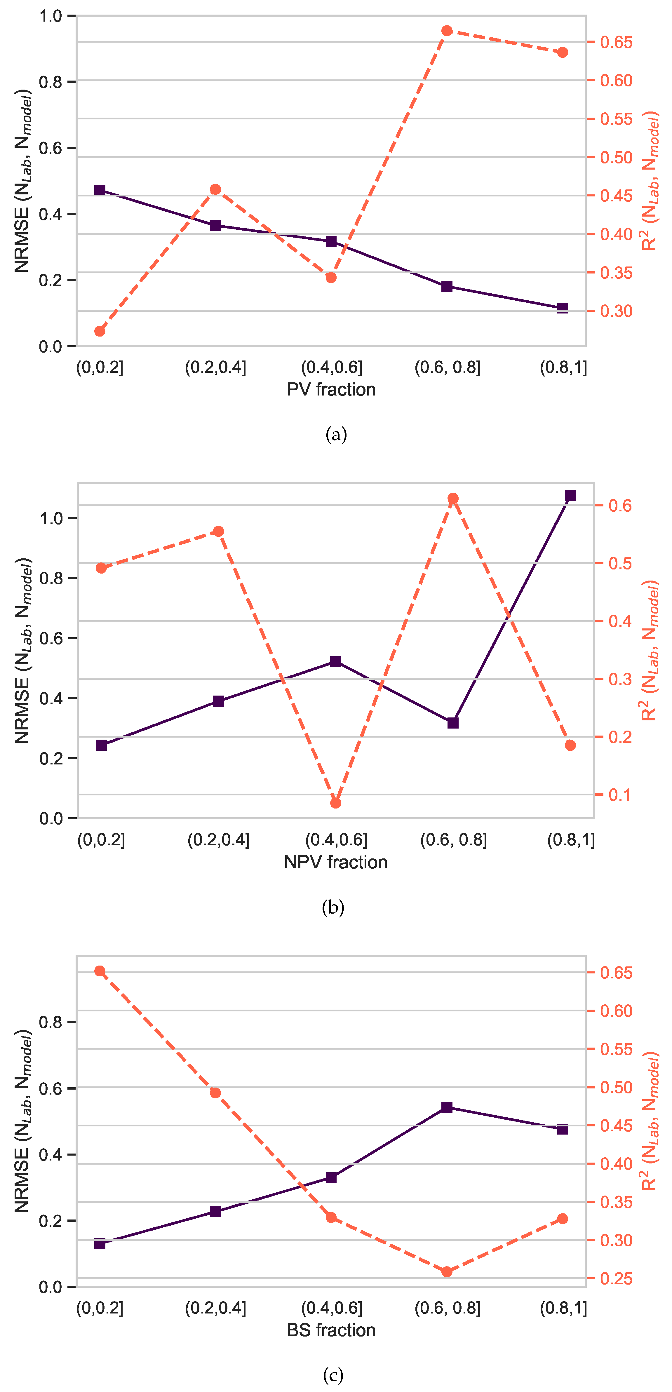
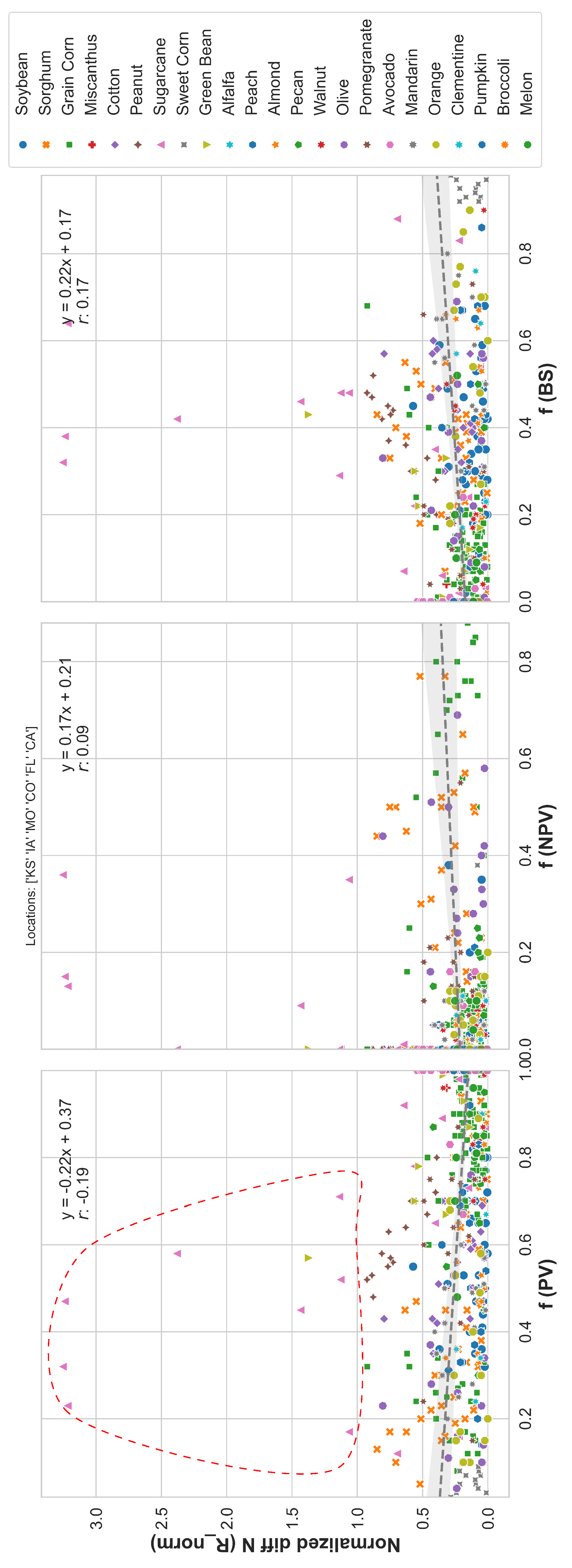
2.5. Cover Fraction Effect on the Estimated Nitrogen

N concentrations in the leaf samples as measured in the laboratory, $N_{lab}$, [24] were compared with N concentrations returned from the fitted PLSR model, $N_{model}$. To assess how the model performance changed as proportional cover of each of the three AutoMCU endmembers, PV, NPV, and BS, we binned the samples falling within 5 bins ((0, 0.2], (0.2, 0.4], (0.4, 0.6], (0.6, 0.8], and (0.8, 1.0]) of each of the three endmembers PV, NPV, and BS. Model performance for each of the bins was assessed using two metrics, normalized $RMSE$ ($NRMSE$), i.e., $RMSE$ divided by the range of observation, and $R^2$, applied to all samples within a bin.

We also investigated the relative effect of changes in cover fractions of each of the three endmembers to better understand the causes of model performance losses. To do so, we modeled changes in residual error as a function of these fractional cover values. Residuals were first transformed by computing a normalized difference between $N_{lab}$ and $N_{model}$ for each sample relative to $N_{lab}$ using Equation (2):

$$R_{norm}=\frac{abs(N_{model}-N_{lab})}{N_{lab}}$$

(2)

To determine the relative influence of each cover fraction on $R_{norm}$, a random forest (RF) regressor algorithm was employed, using the scikit-learn Python package. The input features used for prediction were the estimated PV, NPV, and BS cover fractions and the output was $R_{norm}$. We used a train/test split of 80%/20%. The random forest model consists of several hyperparameters that need to be fine-tuned. We used a grid optimization approach where the model was fit using 10-fold cross-validation for each combination of candidate values for four hyperparameters (

Table 2. List of candidate values for hyperparameters for the RF model.

RF Parameters	Tested Values
n-estimator	[10, 50, 100, 200, 300, 500, 700, 1000, 1500, 2000]
max-tree-depth	[10, 30, 50, 70, 100, 150, 200]
min-samples-split	[2, 3, 4, 5, 8, 10]
min-samples-leaf	[1, 2, 3, 4, 5]

). These hyperparameters included the number of trees in the forest (n-estimator), (b) the maximum depth of the trees, (c) the minimum number of samples required for node splitting (min-samples-split), and (d) the minimum number of samples required at a leaf node (min-samples-leaf). The hyperparameter combination resulting in the best cross-validation performance was kept, and the RF model was trained to the full dataset using these optimized parameters. After building the RF model, the feature importance for the prediction of $R_{norm}$ was computed for each of the three main endmembers, $f\left(PV\right)$, $f\left(NPV\right)$, and $f\left(BS\right)$.

3. Results and Discussion

While validation of the AutoMCU algorithm is outside of the scope of this study because of a sufficient amount of prior research and publication, we found that the AutoMCU algorithm produced values of endmember cover fraction that were highly consistent with field observations (Figure 5). Maps produced by the algorithm matched well with the expected spatial arrangement of the different cover types (Figure 6), and we found no reason to doubt that the AutoMCU algorithm successfully identified and distinguished between PV, NPV, and BS in the spectrometer imagery for the purposes of evaluating their effects on nitrogen content estimation.

We found that cover fractions of each of the three endmembers varied by crop species and location (Figure 7). The highest median values for $f\left(PV\right)$ were found in fields planted with green bean, pecan, and grain corn crops. Similarly, olive had the highest median value for $f\left(NPV\right)$, and sweet corn and melon shared the highest median values of $f\left(BS\right)$. Among the crops, grain corn showed the largest diversity of cover values, largely due to crop age as a result of it being planted across all three field campaigns. Approximately 21% of the pixels exhibited $f\left(PV\right)$ exceeding 0.9, while 62% of the pixels showed $f\left(PV\right)$ surpassing 0.5. Conversely, the analysis revealed that $f\left(NPV\right)$ values exceeding 0.5 were observed in only 5% of the pixels, primarily concentrated in grain corn farms. Moreover, approximately 20% of the pixels displayed $f\left(BS\right)$ values surpassing 0.5, with sweet corn and sorghum crops being the primary contributors to this category.

Impact of Cover Fractions on the Estimated Nitrogen

The performance of the PLSR N content model was strongly affected by variations in the proportional cover of the three endmembers, PV, NPV, and BS. As PV cover decreased from >80% to <20%, $R^2$ values declined from 0.64 to 0.03 and $NRMSE$ decreased from 0.46 to 0.11 (Figure 8a). This was the expected result since PV corresponds to the photosynthetically active plant material that is more likely to accumulate nitrogen. However, no relationship was found between NPV fraction variations and PLSR model performance (Figure 8b). In parallel, a decrease in BS fraction was associated with an increase in model performance (Figure 8c), with the sharpest reduction in $R^2$, occurring with BS between 0.6 and 0.8. Generally, as $f\left(BS\right)$ increased, $NRMSE$ values also increased except for the $f\left(BS\right)$ values within the last range (0.8, 1]. The obtained results in this study support the findings of the previous research conducted in [24], which focused on investigating the influence of the Normalized Difference Vegetation Index (NDVI), a vegetation metric loosely correlated with PV fraction, on the accuracy of nitrogen estimation using the PLSR method.

Looking at the normalized residuals (Equation (2)), a similar pattern unfolded. Regression lines fit to $R_{norm}$ values against the fractional cover values had a negative slope for PV fraction (smaller $R_{norm}$ equates to a lower variation in the residuals) and positive slopes for both NPV and BS (Figure 9). This suggests that the estimated N in image pixels with a higher $f\left(PV\right)$ was closer to the lab-measured concentration from leaf samples. In comparison, a positive correlation was observed between both $f\left(BS\right)$ and $f\left(NPV\right)$ values and the $R_{norm}$. Thus, as the $f\left(BS\right)$ values increased in mixed pixels, the performance of the PLSR model weakened in estimating crop canopy N. However, correlation coefficients were relatively small in all cases, likely due to a moderate number of extreme outliers. The outlier data points exhibiting $R_{norm}$ values greater than 1 (shown in the red closed curve in Figure 9) occurred mainly when $f\left(PV\right)$ was less than 0.6 and $f\left(BS\right)$ was greater than 0.4. Notably, the relationship between $f\left(NPV\right)$ and $R_{norm}$ was the weakest of the three, likely a result of the fact that NPV can also contain smaller (but detectable) amounts of N compared with PV [42,43]. In contrast, BS is composed of soil and other nonvegetated materials that typically have lower nitrogen content.

We were unable to identify a pattern between crop species and $R_{norm}$ (colors/shapes in Figure 9). The same general trend was dominated by cover fractions rather than any species-specific differences in N allocation, indicating that the fitted model found spectral features showing N response independent of species. The impact of the cover fraction on Rnorm highlights the importance of accounting for vegetation cover when estimating crop nutrient content from spectral reflectance, $f\left(PV\right)$ can significantly impact the spectral response of pixels over agricultural lands, while significant values of $f\left(BS\right)$ lead to errors in the estimation of crop nutrient content from spectral data.

To find the relative feature importance of $f\left(PV\right)$, $f\left(NPV\right)$, and $f\left(BS\right)$ on estimating $R_{norm}$, an RF model was trained and tested over the dataset. After the cross-validation analysis, we found that the best candidates for n-estimator, max-tree-depth, min-sample-split, and min-sample-leaf were 300, 70, 10, and 5, respectively. The factor importance values revealed that the PV value had the strongest effect on $R_{norm}$ predictions with a score of 0.43 (Figure 10). The next important feature was BS, with a score of 0.30. Finally, NPV was the least important factor, with a score of 0.27, supporting the earlier result that NPV had the lowest correlation with $R_{norm}$ (Figure 9). The elevated feature importance scores of PV and BS suggest that these factors exert a more substantial influence on nitrogen content estimation from a mixed pixel than NPV. Increasing BS had a stronger effect on model performance than increasing NPV in multiple tests, suggesting the problem might have less to do with the addition of confusing spectral features than a simple reduction in features important to N retrieval.

4. Conclusions

We quantified the effect of mixed pixel fraction on partial least squares regression (PLSR) model estimates of canopy N content. We found that the pixel area covered with photosynthetic vegetation, $f\left(PV\right)$, had the strongest effect on PLSR model prediction errors, with increasing cover values associated with lower variation in residuals. Moreover, we found model performance losses were not indifferent to the material that replaced the lost PV cover. The model residuals were more sensitive to increases in bare soil (BS) cover than to increases in non-photosynthetic vegetation (NPV) cover. Importantly, these results appeared to be independent across the four regions of the United States and across 24 species mapped with airborne imaging spectroscopy data.

While our results contribute valuable insights for precision agriculture and demonstrate the potential of remote sensing in the estimation of N in crops, we recognize certain limitations and opportunities for refinement. A primary concern is the accuracy of the PLSR model when applied to mixed pixels, achieving a maximum $R^2$ value of approximately 0.64. This accuracy is contingent upon the proportion of PV and BS within the mixed pixels. Results suggest that while the model can provide useful general insights into nitrogen content across varied cover fractions, its precision may not meet the threshold for all practical applications in precision agriculture.

These findings enhance our understanding of the relationship between cover fractions and crop canopy N estimation, providing new insights for precision agriculture applications. They also demonstrate the potential of remote sensing techniques in providing an estimate of nutrient content across the highly variable cover fractions resulting from coarser resolution spectroscopy data increasingly available from spaceborne instruments. Future research could explore the integration of AutoMCU and PLSR to incorporate the influence of cover fractions into models for estimating N content. In such a way, the accuracy of nitrogen estimation could potentially be further improved, leading to more precise and reliable results.

References

1. Asner, G.P. Biophysical and Biochemical Sources of Variability in Canopy Reflectance. Remote Sens. Environ. 1998, 64, 234–253. [Google Scholar] [CrossRef]
2. Asner, G.P.; Lobell, D.B. A Biogeophysical Approach for Automated SWIR Unmixing of Soils and Vegetation. Remote Sens. Environ. 2000, 74, 99–112. [Google Scholar] [CrossRef]
3. Asner, G.P.; Heidebrecht, K.B. Spectral unmixing of vegetation, soil and dry carbon cover in arid regions: Comparing multispectral and hyperspectral observations. Int. J. Remote Sens. 2002, 23, 3939–3958. [Google Scholar] [CrossRef]
4. Nagler, P.L.; Inoue, Y.; Glenn, E.P.; Russ, A.L.; Daughtry, C.S.T. Cellulose absorption index (CAI) to quantify mixed soil-plant litter scenes. Remote Sens. Environ. 2003, 87, 310–325. [Google Scholar] [CrossRef]
5. Dai, Z.; Ding, Y.; Xu, C.; Chen, Y.; Liu, L. Evaluation of the impact of crop residue on fractional vegetation cover estimation by vegetation indices over conservation tillage cropland: A simulation study. Int. J. Remote Sens. 2022, 43, 6463–6482. [Google Scholar] [CrossRef]
6. Zhao, F.; Xu, B.; Yang, X.; Jin, Y.; Li, J.; Xia, L.; Chen, S.; Ma, H. Remote Sensing Estimates of Grassland Aboveground Biomass Based on MODIS Net Primary Productivity (NPP): A Case Study in the Xilingol Grassland of Northern China. Remote Sens. 2014, 6, 5368–5386. [Google Scholar] [CrossRef]
7. Wang, G.; Wang, J.; Zou, X.; Chai, G.; Wu, M.; Wang, Z. Estimating the fractional cover of photosynthetic vegetation, non-photosynthetic vegetation and bare soil from MODIS data: Assessing the applicability of the NDVI-DFI model in the typical Xilingol grasslands. Int. J. Appl. Earth Obs. Geoinf. 2019, 76, 154–166. [Google Scholar] [CrossRef]
8. Guerschman, J.P.; Hill, M.J.; Renzullo, L.J.; Barrett, D.J.; Marks, A.S.; Botha, E.J. Estimating fractional cover of photosynthetic vegetation, non-photosynthetic vegetation and bare soil in the Australian tropical savanna region upscaling the EO-1 Hyperion and MODIS sensors. Remote Sens. Environ. 2009, 113, 928–945. [Google Scholar] [CrossRef]
9. Guerschman, J.P.; Hill, M.J.; Leys, J.; Heidenreich, S. Vegetation cover dependence on accumulated antecedent precipitation in Australia: Relationships with photosynthetic and non-photosynthetic vegetation fractions. Remote Sens. Environ. 2020, 240, 111670. [Google Scholar] [CrossRef]
10. Bai, X.; Zhao, W.; Ji, S.; Qiao, R.; Dong, C.; Chang, X. Estimating fractional cover of non-photosynthetic vegetation for various grasslands based on CAI and DFI. Ecol. Indic. 2021, 131, 108252. [Google Scholar] [CrossRef]
11. Heylen, R.; Parente, M.; Gader, P. A Review of Nonlinear Hyperspectral Unmixing Methods. IEEE J. Sel. Top. Appl. Earth Obs. Remote Sens. 2014, 7, 1844–1868. [Google Scholar] [CrossRef]
12. Bhatt, J.S.; Joshi, M.V.; Raval, M.S. A data-driven stochastic approach for unmixing hyperspectral imagery. IEEE J. Sel. Top. Appl. Earth Obs. Remote Sens. 2014, 7, 1936–1946. [Google Scholar] [CrossRef]
13. Scheunders, P.; Tuia, D.; Moser, G. Contributions of Machine Learning to Remote Sensing Data Analysis. In Comprehensive Remote Sensing; Liang, S., Ed.; Elsevier: Oxford, UK, 2018; pp. 199–243. [Google Scholar] [CrossRef]
14. Mitraka, Z.; Del Frate, F.; Carbone, F. Nonlinear Spectral Unmixing of Landsat Imagery for Urban Surface Cover Mapping. IEEE J. Sel. Top. Appl. Earth Obs. Remote Sens. 2016, 9, 3340–3350. [Google Scholar] [CrossRef]
15. Tits, L.; De Keersmaecker, W.; Somers, B.; Asner, G.P.; Farifteh, J.; Coppin, P. Hyperspectral shape-based unmixing to improve intra- and interclass variability for forest and agro-ecosystem monitoring. Isprs J. Photogramm. Remote Sens. 2012, 74, 163–174. [Google Scholar] [CrossRef]
16. Ertürk, A.; Plaza, A. Informative Change Detection by Unmixing for Hyperspectral Images. IEEE Geosci. Remote Sens. Lett. 2015, 12, 1252–1256. [Google Scholar] [CrossRef]
17. Iordache, M.D.; Tits, L.; Bioucas-Dias, J.M.; Plaza, A.; Somers, B. A Dynamic Unmixing Framework for Plant Production System Monitoring. IEEE J. Sel. Top. Appl. Earth Obs. Remote Sens. 2014, 7, 2016–2034. [Google Scholar] [CrossRef]
18. Aulakh, M.S.; Malhi, S.S. Interactions of Nitrogen with Other Nutrients and Water: Effect on Crop Yield and Quality, Nutrient Use Efficiency, Carbon Sequestration, and Environmental Pollution; Academic Press: Cambridge, MA, USA, 2005; Volume 86, pp. 341–409. [Google Scholar] [CrossRef]
19. Yao, X.; Zhu, Y.; Tian, Y.; Feng, W.; Cao, W. Exploring hyperspectral bands and estimation indices for leaf nitrogen accumulation in wheat. Int. J. Appl. Earth Obs. Geoinf. 2010, 12, 89–100. [Google Scholar] [CrossRef]
20. Feng, W.; Zhang, H.Y.; Zhang, Y.S.; Qi, S.L.; Heng, Y.R.; Guo, B.B.; Ma, D.Y.; Guo, T.C. Remote detection of canopy leaf nitrogen concentration in winter wheat by using water resistance vegetation indices from in-situ hyperspectral data. Field Crop. Res. 2016, 198, 238–246. [Google Scholar] [CrossRef]
21. Dashti, H.; Glenn, N.; Ustin, S.; Mitchell, J.; Qi, Y.; Ilangakoon, N.; Flores, A.; Silván-Cárdenas, J.; Zhao, K.; Spaete, L.P.; et al. Empirical methods for remote sensing of nitrogen in drylands may lead to unreliable interpretation of ecosystem function. IEEE Trans. Geosci. Remote Sens. 2019, 57, 3993–4004. [Google Scholar] [CrossRef]
22. Fu, Y.; Yang, G.; Pu, R.; Li, Z.; Li, H.; Xu, X.; Song, X.; Yang, X.; Zhao, C. An overview of crop nitrogen status assessment using hyperspectral remote sensing: Current status and perspectives. Eur. J. Agron. 2021, 124, 126241. [Google Scholar] [CrossRef]
23. Clevers, J.G.; Kooistra, L. Using hyperspectral remote sensing data for retrieving canopy chlorophyll and nitrogen content. IEEE J. Sel. Top. Appl. Earth Obs. Remote Sens. 2012, 5, 574–583. [Google Scholar] [CrossRef]
24. Dai, J.; Jamalinia, E.; Vaughn, N.R.; Martin, R.E.; König, M.; Hondula, K.L.; Calhoun, J.; Heckler, J.; Asner, G.P. A general methodology for the quantification of crop canopy nitrogen across diverse species using airborne imaging spectroscopy. Remote Sens. Environ. 2023, 298, 113836. [Google Scholar] [CrossRef]
25. Asner, G.P.; Martin, R.E.; Anderson, C.B.; Knapp, D.E. Quantifying forest canopy traits: Imaging spectroscopy versus field survey. Remote Sens. Environ. 2015, 158, 15–27. [Google Scholar] [CrossRef]
26. Chen, L.; Zhang, Y.; Nunes, M.H.; Stoddart, J.; Khoury, S.; Chan, A.H.; Coomes, D.A. Predicting leaf traits of temperate broadleaf deciduous trees from hyperspectral reflectance: Can a general model be applied across a growing season? Remote Sens. Environ. 2022, 269, 112767. [Google Scholar] [CrossRef]
27. Asner, G.; Dai, J.; Hondula, K.; Jamalinia, E.; Konig, M.; Martin, P.; Vaughn, N.; Guido, J.; Shivers, S.; Duren, R.; et al. Land and Ocean Applications and Approaches for the Carbon Mapper Satellite Mission. In Proceedings of the American Geophysical Union Fall Meeting, AGU, Chicago, IL, USA, 12–16 December 2022. [Google Scholar]
28. Imaging, A.; Geophysics, L. ACORN user’s guide, stand alone version. Anal. Imaging Geophys. LLC 2001, 64. [Google Scholar]
29. Roberts, D.; Smith, M.; Adams, J. Green vegetation, nonphotosynthetic vegetation, and soils in AVIRIS data. Remote Sens. Environ. 1993, 44, 255–269. [Google Scholar] [CrossRef]
30. Lobell, D.B.; Asner, G.P. Cropland distributions from temporal unmixing of MODIS data. Remote Sens. Environ. 2004, 93, 412–422. [Google Scholar] [CrossRef]
31. Lobell, D.B.; Asner, G.P.; Law, B.E.; Treuhaft, R.N. Subpixel canopy cover estimation of coniferous forests in Oregon using SWIR imaging spectrometry. J. Geophys. Res. Atmos. 2001, 106, 5151–5160. [Google Scholar] [CrossRef]
32. Jamalinia, E.; Dai, J.; Vaughn, N.; Hondula, K.; König, M.; Heckler, J.; Asner, G. Application of Imaging Spectroscopy to Quantify Fractional Cover Over Agricultural Lands. In Proceedings of the IGARSS 2023—2023 IEEE International Geoscience and Remote Sensing Symposium, Pasadena, CA, USA, 16–21 July 2023; pp. 681–684. [Google Scholar] [CrossRef]
33. Survey, U.S.G.; Kokaly, R.F.; Clark, R.N.; Swayze, G.A.; Livo, K.E.; Hoefen, T.M.; Pearson, N.C.; Wise, R.A.; Benzel, W.; Lowers, H.A.; et al. Usgs Spectral Library Version 7 Data: Us Geological Survey Data Release; Technical Report; United States Geological Survey (USGS): Reston, VA, USA, 2017. [CrossRef]
34. Baldridge, A.; Hook, S.; Grove, C.; Rivera, G. The ASTER spectral library version 2.0. Remote Sens. Environ. 2009, 113, 711–715. [Google Scholar] [CrossRef]
35. Meerdink, S.K.; Hook, S.J.; Roberts, D.A.; Abbott, E.A. The ECOSTRESS spectral library version 1.0. Remote Sens. Environ. 2019, 230, 111196. [Google Scholar] [CrossRef]
36. Martin, R.E.; Chadwick, K.D.; Brodrick, P.G.; Carranza-Jimenez, L.; Vaughn, N.R.; Asner, G.P. An approach for foliar trait retrieval from airborne imaging spectroscopy of tropical forests. Remote Sens. 2018, 10, 199. [Google Scholar] [CrossRef]
37. Burnett, A.C.; Anderson, J.; Davidson, K.J.; Ely, K.S.; Lamour, J.; Li, Q.; Morrison, B.D.; Yang, D.; Rogers, A.; Serbin, S.P. A best-practice guide to predicting plant traits from leaf-level hyperspectral data using partial least squares regression. J. Exp. Bot. 2021, 72, 6175–6189. [Google Scholar] [CrossRef] [PubMed]
38. Wang, Z.; Chlus, A.; Geygan, R.; Ye, Z.; Zheng, T.; Singh, A.; Couture, J.J.; Cavender-Bares, J.; Kruger, E.L.; Townsend, P.A. Foliar functional traits from imaging spectroscopy across biomes in eastern North America. New Phytol. 2020, 228, 494–511. [Google Scholar] [CrossRef] [PubMed]
39. Wu, J.; Chavana-Bryant, C.; Prohaska, N.; Serbin, S.P.; Guan, K.; Albert, L.P.; Yang, X.; van Leeuwen, W.J.D.; Garnello, A.J.; Martins, G.; et al. Convergence in relationships between leaf traits, spectra and age across diverse canopy environments and two contrasting tropical forests. New Phytol. 2017, 214, 1033–1048. [Google Scholar] [CrossRef] [PubMed]
40. Serbin, S.P.; Wu, J.; Ely, K.S.; Kruger, E.L.; Townsend, P.A.; Meng, R.; Wolfe, B.T.; Chlus, A.; Wang, Z.; Rogers, A. From the Arctic to the tropics: Multibiome prediction of leaf mass per area using leaf reflectance. New Phytol. 2019, 224, 1557–1568. [Google Scholar] [CrossRef]
41. Vaughn, N.; Asner, G. PLSR. 2023. Available online: https://zenodo.org/records/7967292 (accessed on 24 May 2023).
42. Evans, J.R. Photosynthesis and nitrogen relationships in leaves of C3 plants. Oecologia 1989, 78, 9–19. [Google Scholar] [CrossRef]
43. Mu, X.; Chen, Y. The physiological response of photosynthesis to nitrogen deficiency. Plant Physiol. Biochem. 2021, 158, 76–82. [Google Scholar] [CrossRef]
Figure 1. Geographical locations of study sites in the contiguous United States, with relative field sampling dates (month/day) and crop species labeled. All fieldwork was conducted in the year 2022 (modified from [24]).
Remotesensing 16 01382 g001
Figure 2. Flow chart of AutoMCU algorithm from [3].
Remotesensing 16 01382 g002
Figure 3. Example spectra for the three classes separated by the AutoMCU algorithm. Band windows used in unmixing are shown in gray.
Remotesensing 16 01382 g003
Figure 4. Example of tied spectra within the VIS and SWIR band window used by the AutoMCU algorithm for the 3 selected endmembers: PV, NPV, and BS. For each endmember, 10 samples of spectra are shown.
Remotesensing 16 01382 g004
Figure 5. AutoMCU estimates of the endmember cover fractions for two example sample points in the studied field locations: (a) soybean in Iowa; (b) sorghum in Kansas.
Remotesensing 16 01382 g005
Figure 6. An example of the flight line images from the Iowa farm used in the study: Maps are (a) the GAO VSWIR reflectance image showing bands for red (650 nm) and green (550 nm), and blue (460 nm) and (b) the resulting fractional cover map from the AutoMCU algorithm as a false-color representation using red = non-photosynthetic vegetation, green = photosynthetic vegetation, and blue = bare soil.
Remotesensing 16 01382 g006
Figure 7. Boxplot showing the cover fractions for the pixels that contain the leaf samples, for photosynthetic vegetation fraction, f ( P V ) ; non-photosynthetic vegetation fraction, f ( N P V ) ; and bare soil fraction, f ( B S ) . Each crop type is presented in different colors.
Remotesensing 16 01382 g007
Figure 8. PLSR model performance to estimate N for various (a) PV fractions, (b) NPV fractions, and (c) BS fractions. The solid dark line and the dashed red line represent N R M S E and R 2 , respectively.
Remotesensing 16 01382 g008
Figure 9. Relation between nitrogen (N) concentration from PLSR model and lab measurements from the samples gathered from agricultural lands.
Remotesensing 16 01382 g009
Figure 10. Feature importance plot, presenting the impact of each cover fraction on the R n o r m .
Remotesensing 16 01382 g010