
Assessing Groundwater Sustainability in the Arabian Peninsula and Its Impact on Gravity Fields through Gravity Recovery and Climate Experiment Measurements


Abstract
:1. Introduction
2. Materials and Methods
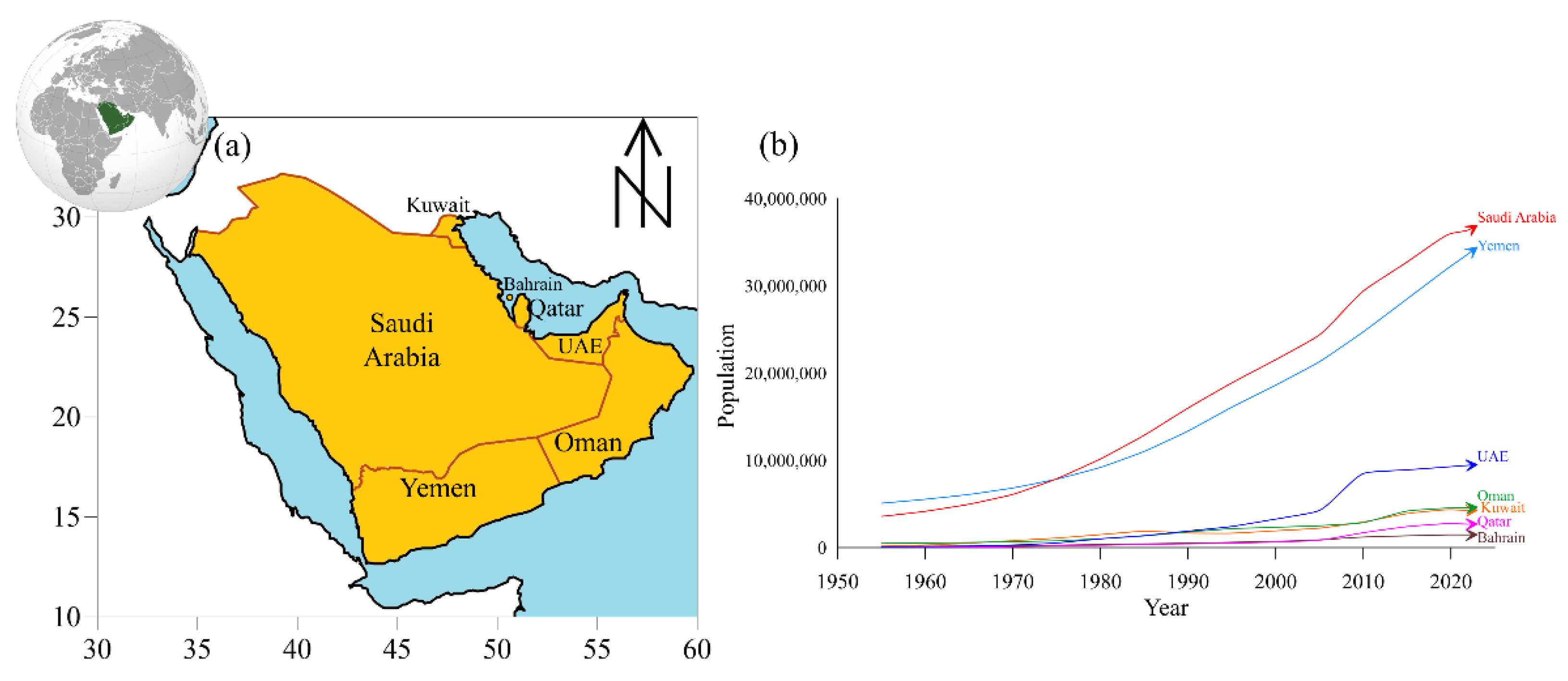
2.1. Study Area
2.2. Data Used
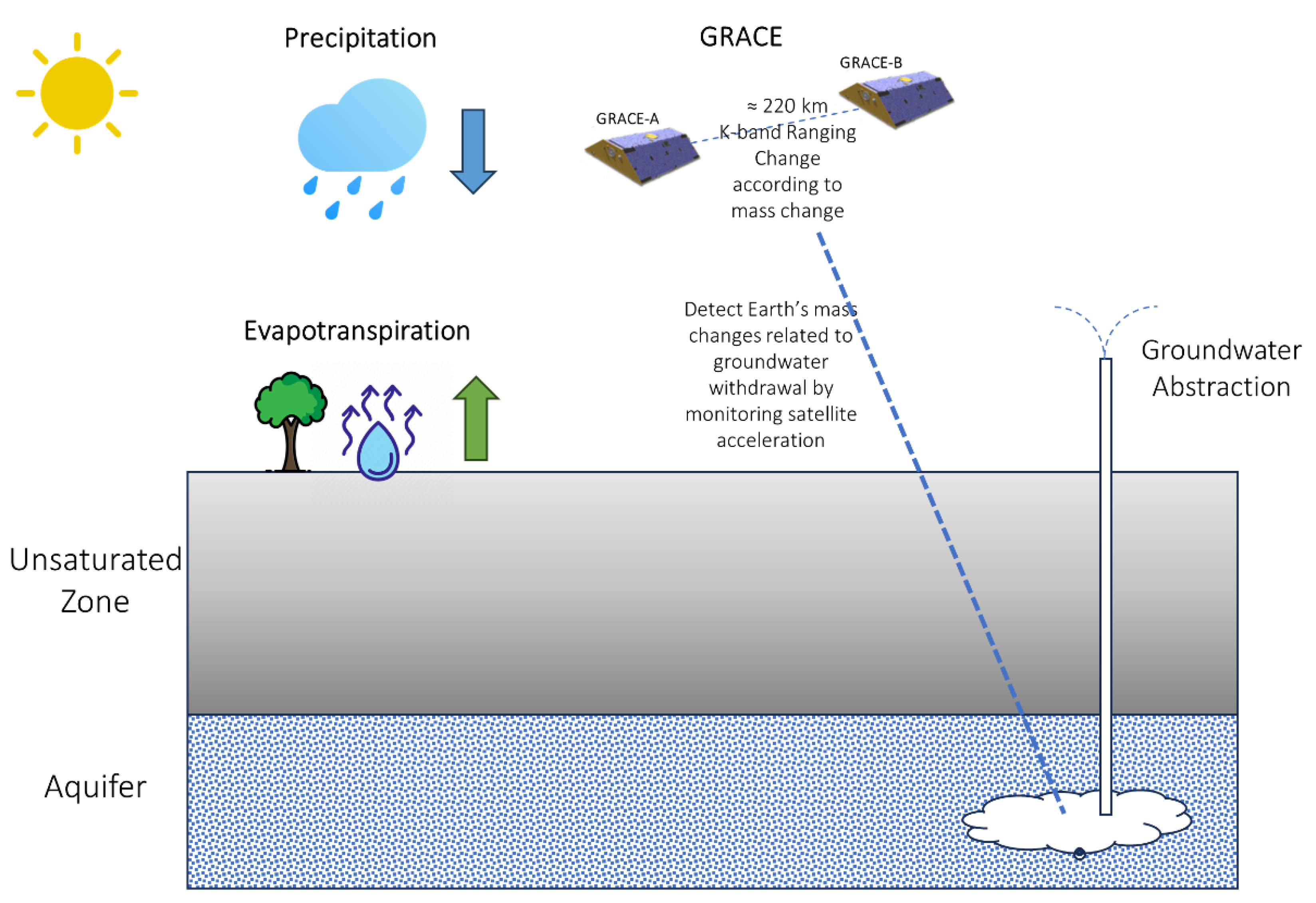
2.2.1. GRACE Data
2.2.2. Hydrological Models
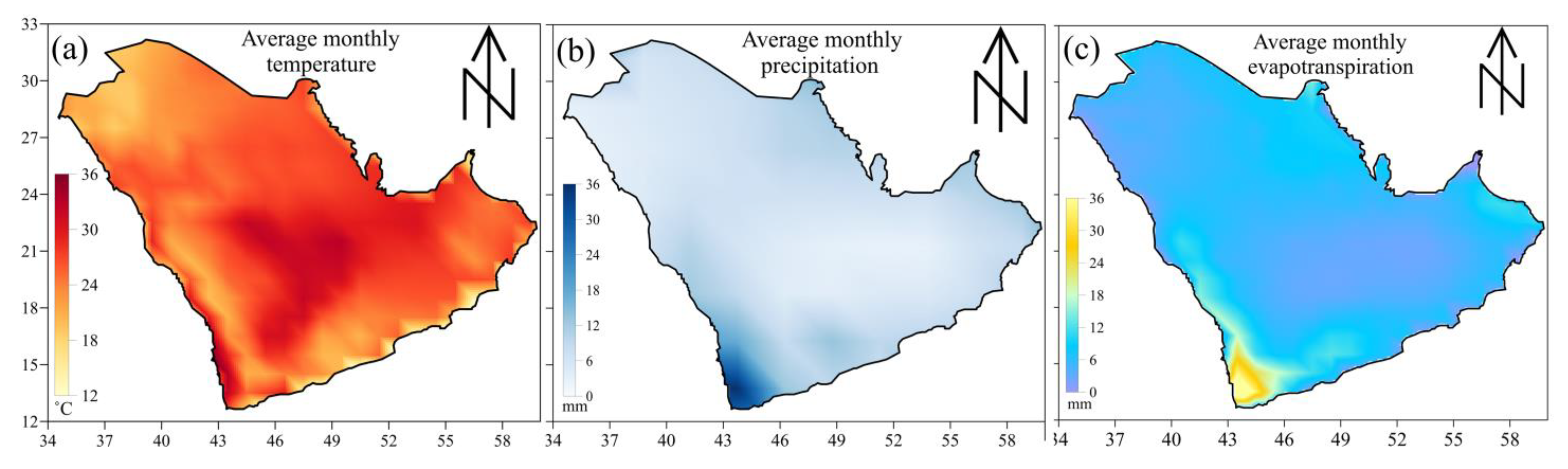
2.2.3. Meteorological Data
3. Methodology
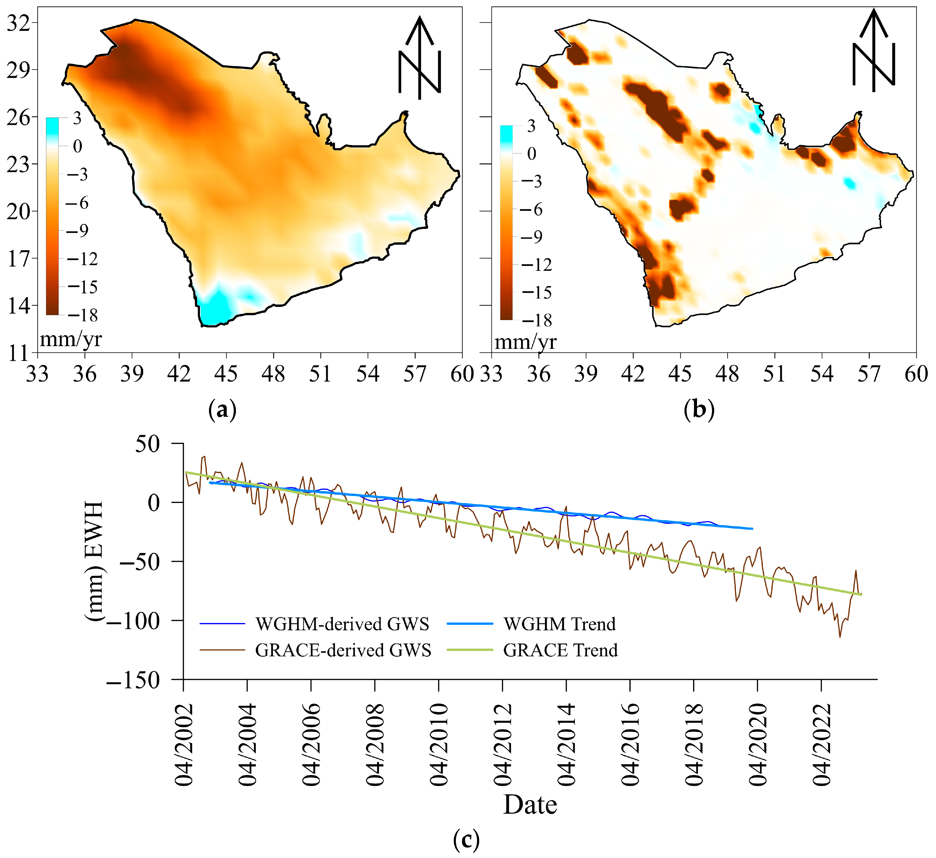
3.1. GWS Estimation
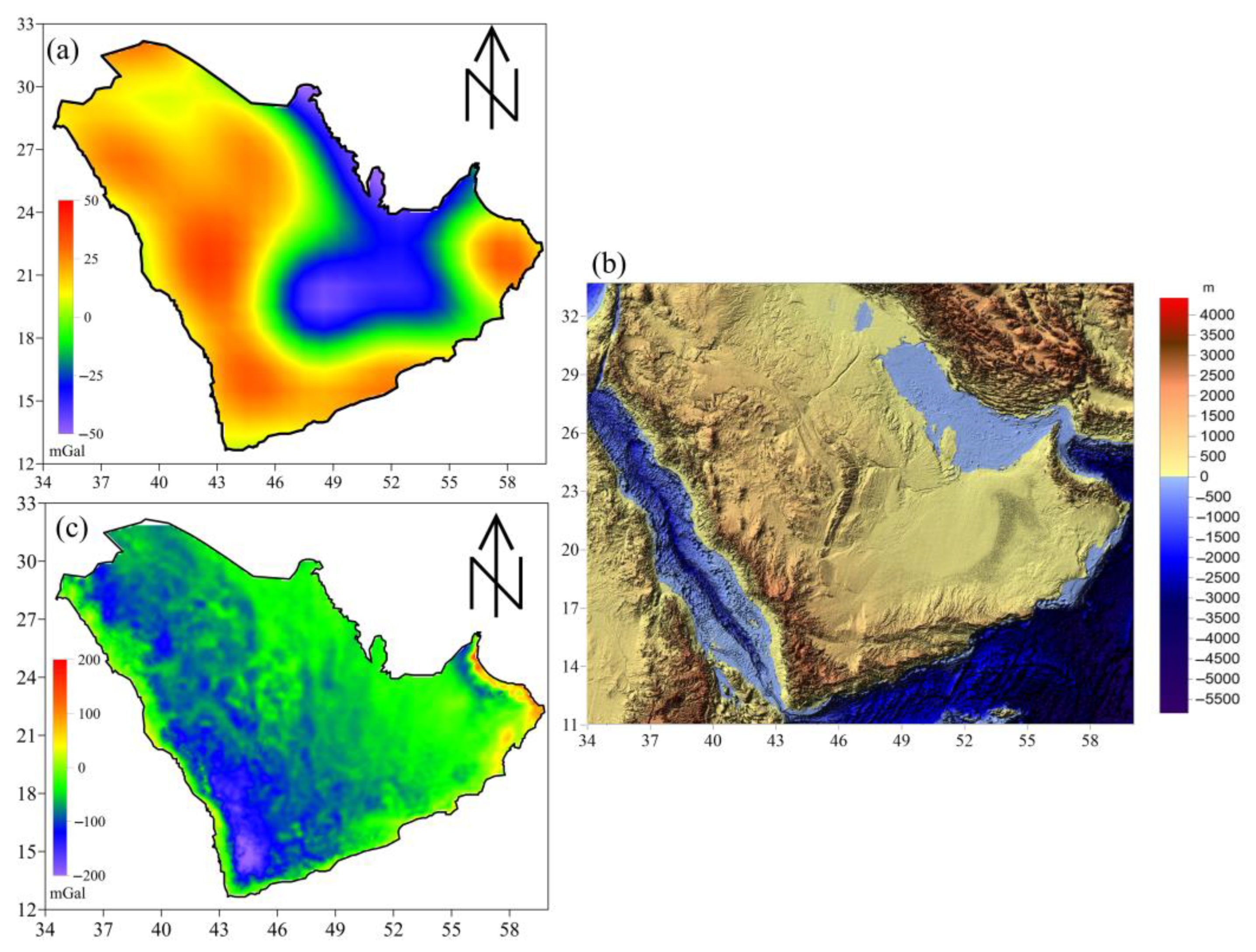
3.2. Gravity Anomaly (GA)
3.3. Seasonal AutoRegressive Integrated Moving Average Model (SARIMA)
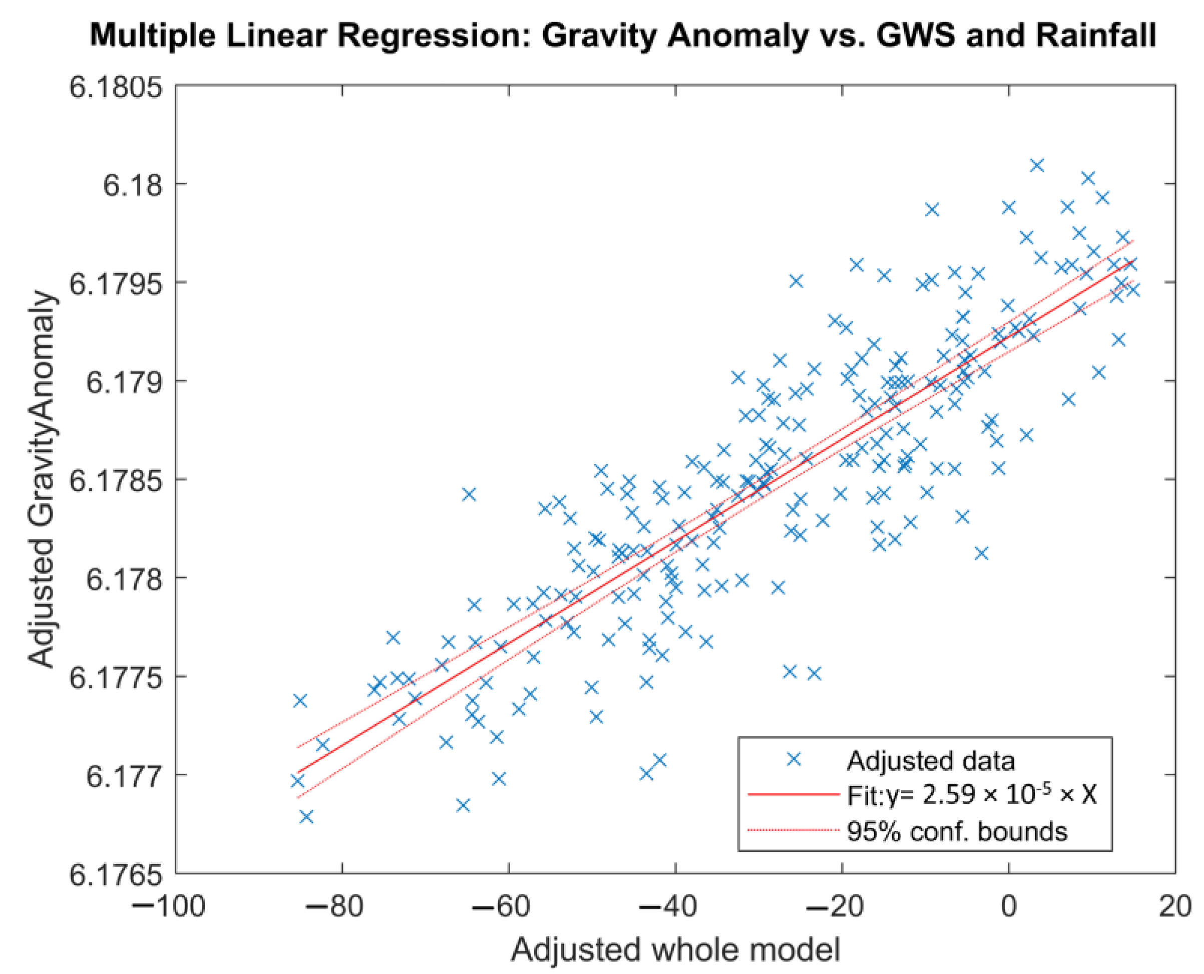
3.4. Multi-Linear Regression Analysis
4. Results and Discussion
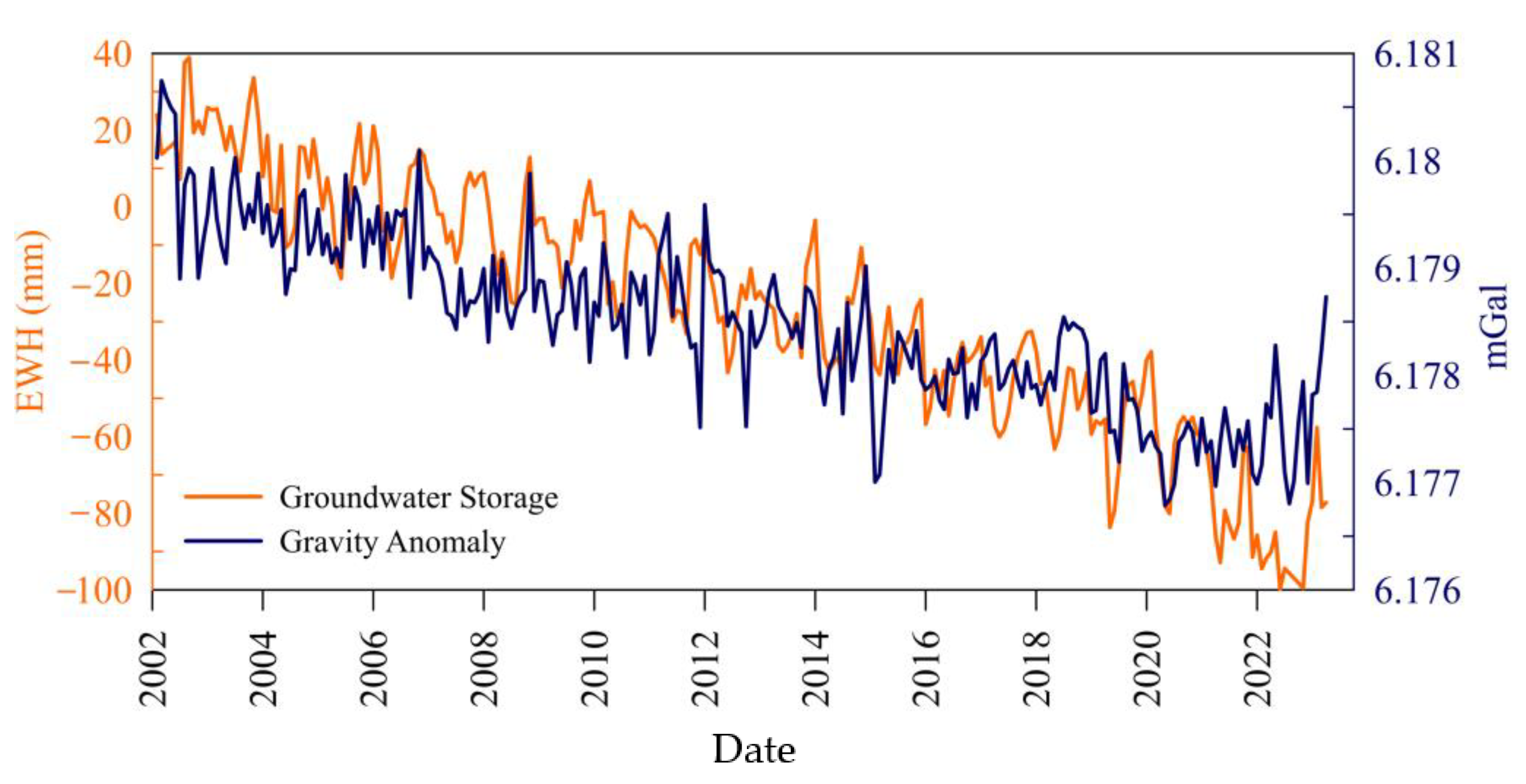
4.1. The GWS Effects on Gravity Anomaly
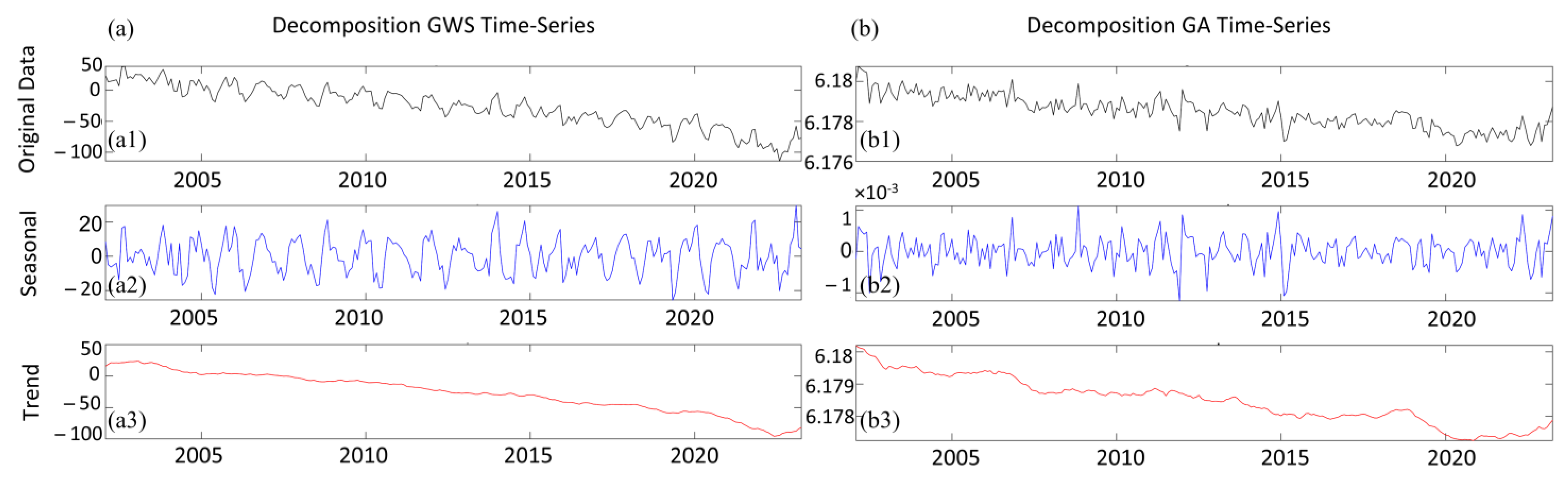
4.2. GWS Seasonal Analysis
4.3. Climate Factors Effect on GWS and GA
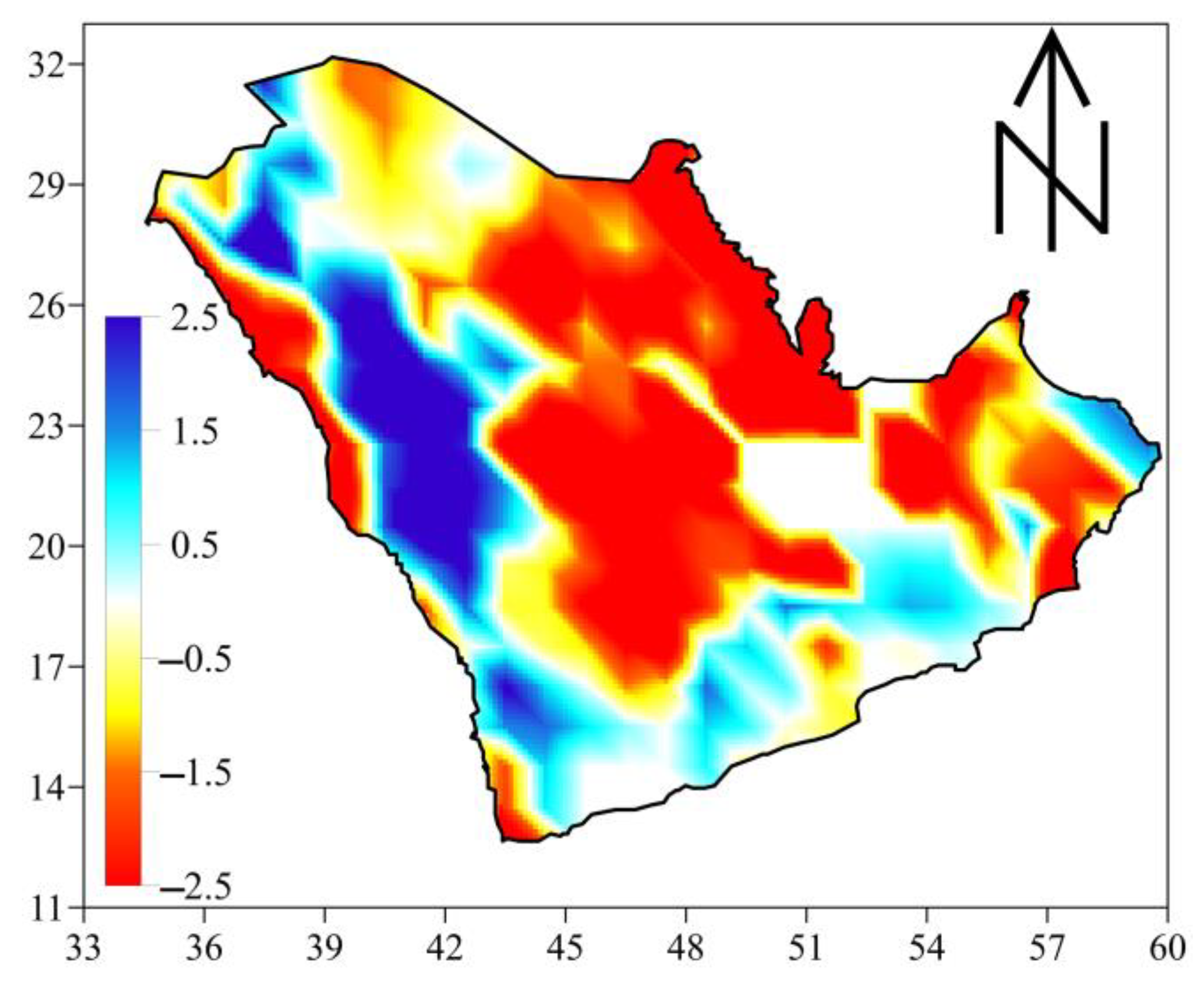
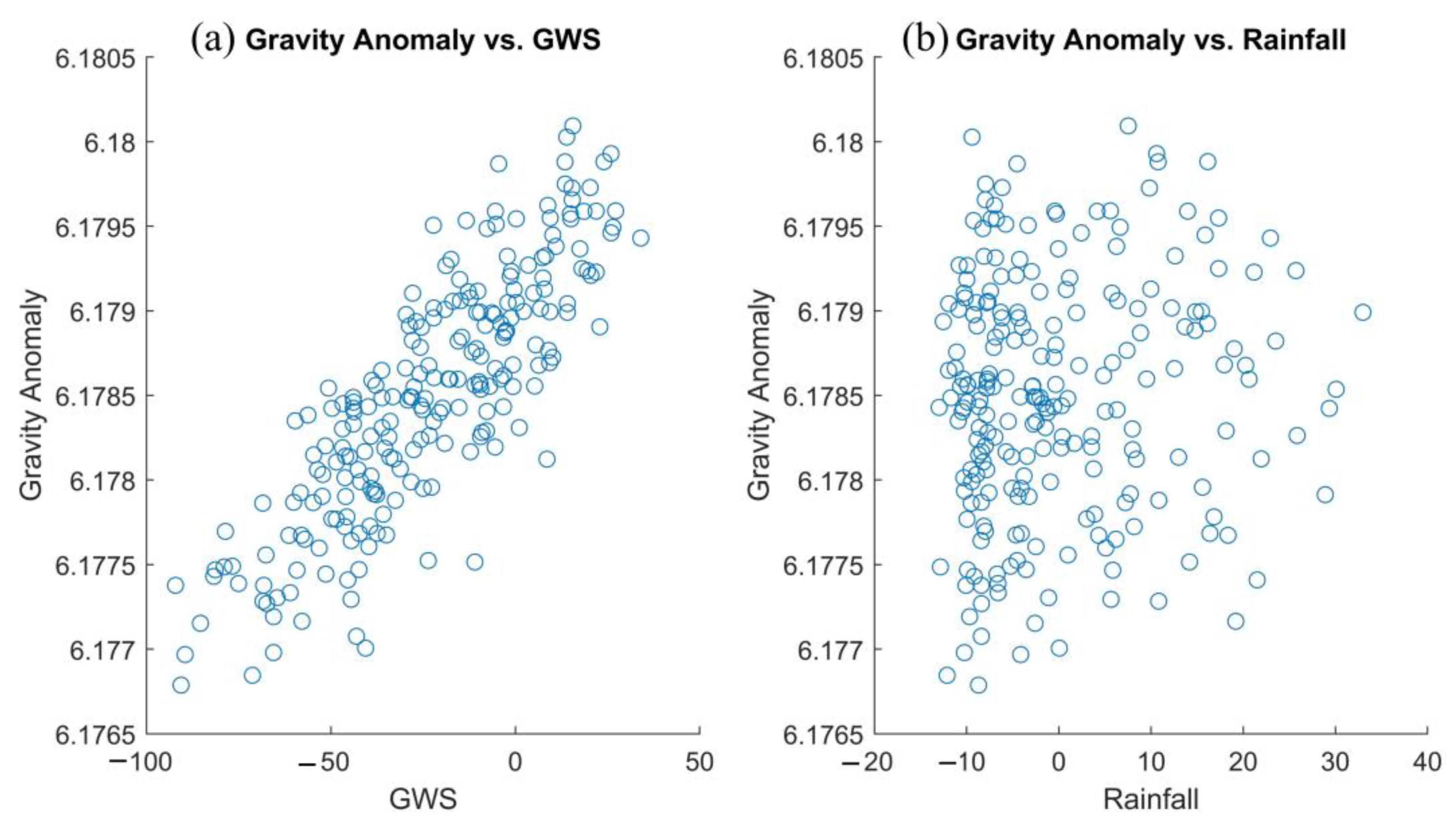
Correlation Analysis
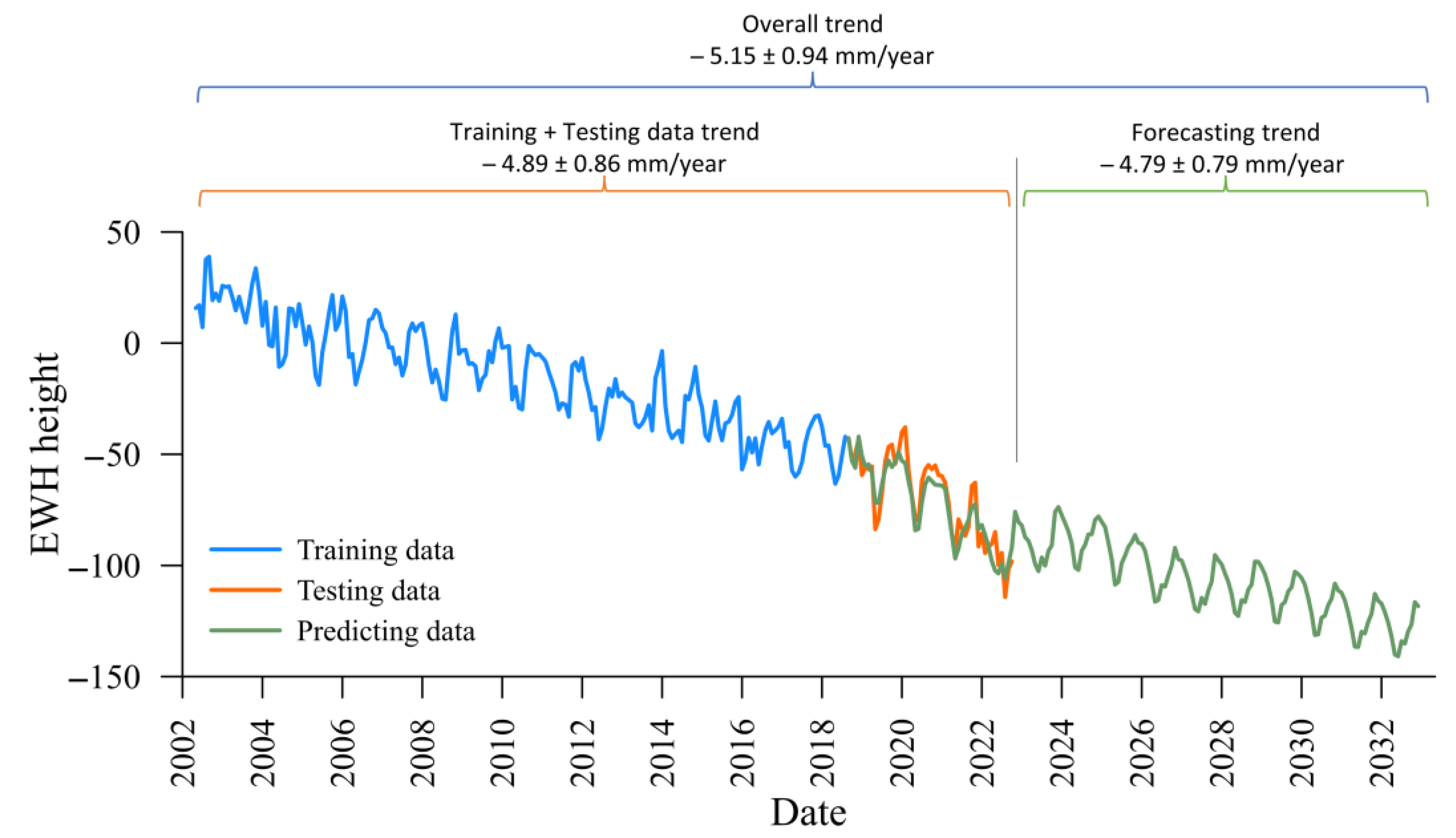
4.4. GWS Prediction
5. Conclusions
Author Contributions
Funding
Data Availability Statement
Acknowledgments
Conflicts of Interest
References
- Hunt, C.E. Thirsty Planet: Strategies for Sustainable Water Management; Academic Foundation: Ahmedabad, India, 2007. [Google Scholar]
- Eyvaz, M.; Wan, Z.; Ahmad, S.; Wan, R. Sustainable Development on Water Resources Management, Policy and Governance in a Changing World; Frontiers Media SA: Lausanne, Switzerland, 2023. [Google Scholar] [CrossRef]
- Shahin, M. Water Resources and Hydrometeorology of the Arab Region; Springer Science & Business Media: New York, NY, USA, 2007; Volume 59. [Google Scholar]
- Tian, Y.; Zheng, Y.; Wu, B.; Wu, X.; Liu, J.; Zheng, C. Modeling surface water-groundwater interaction in arid and semi-arid regions with intensive agriculture. Environ. Model. Softw. 2015, 63, 170–184. [Google Scholar] [CrossRef]
- Sherif, M.; Sefelnasr, A.; Al Rashed, M.; Alshamsi, D.; Zaidi, F.K.; Alghafli, K.; Baig, F.; Al-Turbak, A.; Alfaifi, H.; Loni, O.A. A review of managed aquifer recharge potential in the Middle East and North Africa Region with examples from the Kingdom of Saudi Arabia and the United Arab Emirates. Water 2023, 15, 742. [Google Scholar] [CrossRef]
- Bahri, A. Water reuse in Middle Eastern and North African countries. In Water Reuse: An International Survey of Current PRACTICE, Issues and Needs; IWA Publishing: London, UK, 2008; pp. 27–47. [Google Scholar]
- Khouri, J.; AUDrouby, A.; Gedeon, R.; Salih, A. Groundwater Protection in the Arab Region; IHP: Paris, France, 1995. [Google Scholar]
- Sherif, M.; Liaqat, M.U.; Baig, F.; Al-Rashed, M. Water resources availability, sustainability and challenges in the GCC countries: An overview. Heliyon 2023, 9, e20543. [Google Scholar] [CrossRef]
- Dawoud, M.A. Water Scarcity in the GCC Countries: Challenges and Opportunities. In GRC Research Papers, in GRC Research Papers; Gulf Research Center: Geneva, Switzerland, 2007. [Google Scholar]
- Dolatyar, M.; Gray, T.S.; Dolatyar, M.; Gray, T.S. Water Politics in the Arabian Peninsula. In Water Politics in the Middle East: A Context for Conflict or Co-Operation? Springer: Berlin/Heidelberg, Germany, 2000; pp. 164–205. [Google Scholar] [CrossRef]
- World Bank. A Water Sector Assessment Report on the Countries of the Cooperation Council of the Arab States of the Gulf; World Bank: Washington, DC, USA, 2005. [Google Scholar]
- Wouters, B.; Bonin, J.A.; Chambers, D.P.; Riva, R.E.; Sasgen, I.; Wahr, J. GRACE, time-varying gravity, Earth system dynamics and climate change. Rep. Prog. Phys. 2014, 77, 116801. [Google Scholar] [CrossRef]
- Chen, J. Satellite gravimetry and mass transport in the earth system. Geod. Geodyn. 2019, 10, 402–415. [Google Scholar] [CrossRef]
- Gehman, C.L.; Harry, D.L.; Sanford, W.E.; Stednick, J.D.; Beckman, N.A. Estimating specific yield and storage change in an unconfined aquifer using temporal gravity surveys. Water Resour. Res. 2009, 45, W00D21. [Google Scholar] [CrossRef]
- Al-Rashed, M.F.; Sherif, M.M. Water resources in the GCC countries: An overview. Water Resour. Manag. 2000, 14, 59–75. [Google Scholar] [CrossRef]
- Siebert, S.; Burke, J.; Faures, J.-M.; Frenken, K.; Hoogeveen, J.; Döll, P.; Portmann, F.T. Groundwater use for irrigation–a global inventory. Hydrol. Earth Syst. Sci. 2010, 14, 1863–1880. [Google Scholar] [CrossRef]
- Droogers, P.; Immerzeel, W.; Terink, W.; Hoogeveen, J.; Bierkens, M.; Van Beek, L.; Debele, B. Water resources trends in Middle East and North Africa towards 2050. Hydrol. Earth Syst. Sci. 2012, 16, 3101–3114. [Google Scholar] [CrossRef]
- Odhiambo, G.O. Water scarcity in the Arabian Peninsula and socio-economic implications. Appl. Water Sci. 2017, 7, 2479–2492. [Google Scholar] [CrossRef]
- Tashtush, F.M.; Al-Zubari, W.K.; Al-Haddad, A.S. The Use of Non-Conventional Water Resources in Agriculture in the Gulf Cooperation Council Countries: Key Challenges and Opportunities for the Use of Treated Wastewater. In Biosaline Agriculture as a Climate Change Adaptation for Food Security; Springer: Berlin/Heidelberg, Germany, 2023; pp. 285–322. [Google Scholar] [CrossRef]
- FAO. Review of World Water Resources by Country; Water Reports No. 23; Food & Agriculture Organization of the UN (FAO): Rome, Italy, 2003. [Google Scholar]
- UN-Water (Ed.) Global Annual Assessment of Sanitation and Drinking-Water (GlAAS) 2012 Report: The Challenge of Extending and Sustaining Services; UN: New York, NY, USA, 2012. [Google Scholar]
- Ojha, R.; Ramadas, M.; Govindaraju, R.S. Current and future challenges in groundwater. I: Modeling and management of resources. J. Hydrol. Eng. 2015, 20, A4014007. [Google Scholar] [CrossRef]
- Green, T.R.; Taniguchi, M.; Kooi, H.; Gurdak, J.J.; Allen, D.M.; Hiscock, K.M.; Treidel, H.; Aureli, A. Beneath the surface of global change: Impacts of climate change on groundwater. J. Hydrol. 2011, 405, 532–560. [Google Scholar] [CrossRef]
- Tapley, B.D.; Bettadpur, S.; Ries, J.C.; Thompson, P.F.; Watkins, M.M. GRACE measurements of mass variability in the Earth system. Science 2004, 305, 503–505. [Google Scholar] [CrossRef]
- Kirschner, M.; Massmann, F.-H.; Steinhoff, M. GRACE. In Distributed Space Missions for Earth System Monitoring; Springer: Berlin/Heidelberg, Germany, 2012; pp. 547–574. [Google Scholar] [CrossRef]
- Frappart, F.; Ramillien, G. Monitoring groundwater storage changes using the Gravity Recovery and Climate Experiment (GRACE) satellite mission: A review. Remote Sens. 2018, 10, 829. [Google Scholar] [CrossRef]
- Rodell, M. 11 Satellite Gravimetry. Remote Sensing of Drought: Innovative Monitoring Approaches; CRC Press: Boca Raton, FL, USA, 2012; p. 261. [Google Scholar]
- Seeber, G. Satellite Geodesy; Walter de gruyter: Berlin, Germany, 2003. [Google Scholar] [CrossRef]
- Chen, J.; Famigliett, J.S.; Scanlon, B.R.; Rodell, M. Groundwater storage changes: Present status from GRACE observations. In Remote Sensing and Water Resources; Springer: Berlin/Heidelberg, Germany, 2016; pp. 207–227. [Google Scholar] [CrossRef]
- Mohasseb, H.A.; Shen, W.; Jiao, J.; Wu, Q. Groundwater Storage Variations in the Main Karoo Aquifer Estimated Using GRACE and GPS. Water 2023, 15, 3675. [Google Scholar] [CrossRef]
- Abd-Elmotaal, H.A.; Makhloof, A.; Hassan, A.A.; Mohasseb, H. Preliminary results on the estimation of ground water in Africa using GRACE and hydrological models. In Proceedings of the International Symposium on Gravity, Geoid and Height Systems 2016: Proceedings Organized by IAG Commission 2 and the International Gravity Field Service, Thessaloniki, Greece, 19–23 September 2016; pp. 217–226. [Google Scholar]
- Richey, A.S.; Thomas, B.F.; Lo, M.H.; Reager, J.T.; Famiglietti, J.S.; Voss, K.; Swenson, S.; Rodell, M. Quantifying renewable groundwater stress with GRACE. Water Resour. Res. 2015, 51, 5217–5238. [Google Scholar] [CrossRef]
- Bhanja, S.N.; Mukherjee, A.; Saha, D.; Velicogna, I.; Famiglietti, J.S. Validation of GRACE based groundwater storage anomaly using in-situ groundwater level measurements in India. J. Hydrol. 2016, 543, 729–738. [Google Scholar] [CrossRef]
- Van der Gun, J. Large Aquifer Systems Around the World; The Groundwater Project; University of Guelph: Guelph, ON, Canada, 2022. [Google Scholar] [CrossRef]
- Mohamed, A.; Alarifi, S.S.; Mohammed, M.A. Geophysical monitoring of the groundwater resources in the Southern Arabian Peninsula using satellite gravity data. Alex. Eng. J. 2024, 86, 311–326. [Google Scholar] [CrossRef]
- Wehbe, Y.; Temimi, M. A remote sensing-based assessment of water resources in the Arabian Peninsula. Remote Sens. 2021, 13, 247. [Google Scholar] [CrossRef]
- Alghafli, K.; Shi, X.; Sloan, W.; Shamsudduha, M.; Tang, Q.; Sefelnasr, A.; Ebraheem, A.A. Groundwater recharge estimation using in-situ and GRACE observations in the eastern region of the United Arab Emirates. Sci. Total Environ. 2023, 867, 161489. [Google Scholar] [CrossRef]
- Fallatah, O.A.; Ahmed, M.; Save, H.; Akanda, A.S. Quantifying temporal variations in water resources of a vulnerable middle eastern transboundary aquifer system. Hydrol. Process. 2017, 31, 4081–4091. [Google Scholar] [CrossRef]
- Döll, P.; Müller Schmied, H.; Schuh, C.; Portmann, F.T.; Eicker, A. Global-scale assessment of groundwater depletion and related groundwater abstractions: Combining hydrological modeling with information from well observations and GRACE satellites. Water Resour. Res. 2014, 50, 5698–5720. [Google Scholar] [CrossRef]
- Mohamed, A.; Abdelrahman, K.; Abdelrady, A. Application of time-variable gravity to groundwater storage fluctuations in Saudi Arabia. Front. Earth Sci. 2022, 10, 873352. [Google Scholar] [CrossRef]
- Fallatah, O.A. Groundwater quality patterns and spatiotemporal change in depletion in the regions of the Arabian Shield and Arabian Shelf. Arab. J. Sci. Eng. 2020, 45, 341–350. [Google Scholar] [CrossRef]
- Agarwal, V.; Kumar, A.; Gomes, R.L.; Marsh, S. Monitoring of Ground Movement and Groundwater Changes in London Using InSAR and GRACE. Appl. Sci. 2020, 10, 8599. [Google Scholar] [CrossRef]
- Khanna, P.; Petrovic, A.; Ramdani, A.I.; Homewood, P.; Mettraux, M.; Vahrenkamp, V. Mid-Holocene to present circum-Arabian sea level database: Investigating future coastal ocean inundation risk along the Arabian plate shorelines. Quat. Sci. Rev. 2021, 261, 106959. [Google Scholar] [CrossRef]
- FAO. FAO’s Information System on Water and Agriculture (AQUASTAT); FAO: Rome, Italy, 2007. [Google Scholar]
- UNESCO. Water in a Changing World; UNESCO: Paris, France, 2009. [Google Scholar]
- Al-Eshlah, A.; Al-Rubaidi, H.; Al-Sabri, A. Agriculture’s contribution to solving the water crisis. In Proceedings of the National Conference for the Management and Development of Water Resources in Yemen organized by the Ministry of Agriculture and Irrigation in January, Sana’a, Yemen, 15–17 January 2011. [Google Scholar]
- AlSarmi, S.; Washington, R. Recent observed climate change over the Arabian Peninsula. J. Geophys. Res. Atmos. 2011, 116, D11109. [Google Scholar] [CrossRef]
- Kornfeld, R.P.; Arnold, B.W.; Gross, M.A.; Dahya, N.T.; Klipstein, W.M.; Gath, P.F.; Bettadpur, S. GRACE-FO: The gravity recovery and climate experiment follow-on mission. J. Spacecr. Rocket. 2019, 56, 931–951. [Google Scholar] [CrossRef]
- Li, Z.; Zhang, Z.; Wang, H. On Tide Aliasing in GRACE Time-Variable Gravity Observations. Remote Sens. 2022, 14, 5403. [Google Scholar] [CrossRef]
- Sun, Z.; Long, D.; Yang, W.; Li, X.; Pan, Y. Reconstruction of GRACE data on changes in total water storage over the global land surface and 60 basins. Water Resour. Res. 2020, 56, e2019WR026250. [Google Scholar] [CrossRef]
- Chen, J.; Tapley, B.; Tamisiea, M.E.; Save, H.; Wilson, C.; Bettadpur, S.; Seo, K.W. Error Assessment of GRACE and GRACE Follow-On Mass Change. J. Geophys. Res. Solid Earth 2021, 126, e2021JB022124. [Google Scholar] [CrossRef]
- Swenson, S.; Chambers, D.; Wahr, J. Estimating geocenter variations from a combination of GRACE and ocean model output. J. Geophys. Res. Solid Earth 2008, 113, B08410. [Google Scholar] [CrossRef]
- Swenson, S.; Wahr, J. Post-processing removal of correlated errors in GRACE data. Geophys. Res. Lett. 2006, 33, L08402. [Google Scholar] [CrossRef]
- Rodell, M.; Houser, P.R.; Jambor, U.; Gottschalck, J.; Mitchell, K.; Meng, C.-J.; Arsenault, K.; Cosgrove, B.; Radakovich, J.; Bosilovich, M.; et al. The Global Land Data Assimilation System. Bull. Am. Meteorol. Soc. 2004, 85, 381–394. [Google Scholar] [CrossRef]
- Rui, H.; Beaudoing, H.; Loeser, C. README Document for NASA GLDAS Version 2 Data Products; Goddart Earth Sciences Data and Information Services Center (GES DISC): Greenbelt, MD, USA, 2018. [Google Scholar]
- Beaudoing, H.; Rodell, M. NASA/Gsfc/Hsl. GLDAS Noah Land Surface Model L; Goddard Earth Sciences Data and Information Services Center (GES DISC): Greenbelt, MD, USA, 2020; Volume 4, p. 3. [Google Scholar] [CrossRef]
- Döll, P.; Fiedler, K. Global-scale modeling of groundwater recharge. Hydrol. Earth Syst. Sci. 2008, 12, 863–885. [Google Scholar] [CrossRef]
- Döll, P.; Kaspar, F.; Lehner, B. A global hydrological model for deriving water availability indicators: Model tuning and validation. J. Hydrol. 2003, 270, 105–134. [Google Scholar] [CrossRef]
- Müller Schmied, H.; Cáceres, D.; Eisner, S.; Flörke, M.; Herbert, C.; Niemann, C.; Peiris, T.A.; Popat, E.; Portmann, F.T.; Reinecke, R. The global water resources and use model WaterGAP v2. 2d: Model description and evaluation. Geosci. Model Dev. 2021, 14, 1037–1079. [Google Scholar] [CrossRef]
- Gu, G.; Adler, R.F. Observed variability and trends in global precipitation during 1979–2020. Clim. Dyn. 2022, 61, 131–150. [Google Scholar] [CrossRef]
- Efon, E.; Ngongang, R.D.; Meukaleuni, C.; Wandjie, B.; Zebaze, S.; Lenouo, A.; Valipour, M. Monthly, Seasonal, and Annual Variations of Precipitation and Runoff Over West and Central Africa Using Remote Sensing and Climate Reanalysis. Earth Syst. Environ. 2022, 7, 67–82. [Google Scholar] [CrossRef]
- Seraphin, P.; Gonçalvès, J.; Hamelin, B.; Stieglitz, T.; Deschamps, P. Influence of intensive agriculture and geological heterogeneity on the recharge of an arid aquifer system (Saq–Ram, Arabian Peninsula) inferred from GRACE data. Hydrol. Earth Syst. Sci. 2022, 26, 5757–5771. [Google Scholar] [CrossRef]
- Heiskanen, W.A.; Moritz, H. Physical Geodesy; Book on physical geodesy covering potential theory, gravity fields, gravimetric and astrogeodetic methods, statistical analysis, etc.; Springer: New York, NY, USA, 1967. [Google Scholar] [CrossRef]
- Vanicek, P.; Krakiwsky, E.J. Geodesy: The Concepts; Elsevier: Amsterdam, The Netherlands, 2015. [Google Scholar] [CrossRef]
- Tscherning, C. Determination of sea surface topography from satellite radar altimetry [ocean geoid, ocean circulation, altimeter]. In Proceedings of the Conference on Satellite Based Navigation and Remote Sensing of the Sea, Copenhagen, Denmark, 4 March 1980. [Google Scholar]
- Prista, N.; Diawara, N.; Costa, M.J.; Jones, C.M. Use of SARIMA models to assess data-poor fisheries: A case study with a sciaenid fishery off Portugal. Fish. Bull. 2011, 109, 170–185. [Google Scholar]
- Karim, A.A.; Pardede, E.; Mann, S. A Model Selection Approach for Time Series Forecasting: Incorporating Google Trends Data in Australian Macro Indicators. Entropy 2023, 25, 1144. [Google Scholar] [CrossRef]
- Khashei, M.; Bijari, M.; Hejazi, S.R. Combining seasonal ARIMA models with computational intelligence techniques for time series forecasting. Soft Comput. 2012, 16, 1091–1105. [Google Scholar] [CrossRef]
- Sirisha, U.M.; Belavagi, M.C.; Attigeri, G. Profit prediction using Arima, Sarima and LSTM models in time series forecasting: A Comparison. IEEE Access 2022, 10, 124715–124727. [Google Scholar] [CrossRef]
- Samal, K.K.R.; Babu, K.S.; Das, S.K.; Acharaya, A. Time series based air pollution forecasting using SARIMA and prophet model. In Proceedings of the 2019 International Conference on Information Technology and Computer Communications, Singapore, 16–18 August 2019; pp. 80–85. [Google Scholar]
- Sun, A.Y.; Scanlon, B.R.; Save, H.; Rateb, A. Reconstruction of GRACE total water storage through automated machine learning. Water Resour. Res. 2021, 57, e2020WR028666. [Google Scholar] [CrossRef]
- Dhulipala, S.; Patil, G.R. Freight production of agricultural commodities in India using multiple linear regression and generalized additive modelling. Transp. Policy 2020, 97, 245–258. [Google Scholar] [CrossRef]
- Konasani, V.R.; Kadre, S.; Konasani, V.R.; Kadre, S. Multiple regression analysis. In Practical Business Analytics Using SAS: A Hands-on Guide; Springer: Berlin/Heidelberg, Germany, 2015; pp. 351–399. [Google Scholar] [CrossRef]
- Schumacher, M.; Forootan, E.; van Dijk, A.I.; Schmied, H.M.; Crosbie, R.S.; Kusche, J.; Döll, P. Improving drought simulations within the Murray-Darling Basin by combined calibration/assimilation of GRACE data into the WaterGAP Global Hydrology Model. Remote Sens. Environ. 2018, 204, 212–228. [Google Scholar] [CrossRef]
- Ziese, M.; Schneider, U.; Meyer-Christoffer, A.; Schamm, K.; Vido, J.; Finger, P.; Bissolli, P.; Pietzsch, S.; Becker, A. The GPCC Drought Index–a new, combined and gridded global drought index. Earth Syst. Sci. Data 2014, 6, 285–295. [Google Scholar] [CrossRef]
- Lloyd-Hughes, B.; Saunders, M.A. A drought climatology for Europe. Int. J. Climatol. A J. R. Meteorol. Soc. 2002, 22, 1571–1592. [Google Scholar] [CrossRef]


| Country | Area (km2) | Population 2023 (Million) |
|---|---|---|
| Bahrain | 652 | 1.491 |
| Kuwait | 17,818 | 4.328 |
| Oman | 212,460 | 4.676 |
| Qatar | 11,610 | 2.726 |
| Saudi Arabia | 2,149,690 | 37.189 |
| UAE | 83,600 | 9511 |
| Yemen | 555,001 | 34,800 |
| Total | 3,030,831 | 94.721 |
| GWS | GWS Trend (mm/Year) | GWS Depletion (km3/Year) 2002–2023 | Average Prec. (mm/Year) 2002–2023 | Average ET (mm/Year) 2002–2023 | |
|---|---|---|---|---|---|
| 2002–2019 | 2002–2023 | ||||
| GRACE-derived GWS | −4.41 ± 0.81 | −4.89 ± 0.86 | −14.82 ± 2.61 | 95.88 ± 0.50 | 80.88 ± 0.61 |
| WGHM-derived GWS | −3.30 ± 0.67 | ___ | |||
Disclaimer/Publisher’s Note: The statements, opinions and data contained in all publications are solely those of the individual author(s) and contributor(s) and not of MDPI and/or the editor(s). MDPI and/or the editor(s) disclaim responsibility for any injury to people or property resulting from any ideas, methods, instructions or products referred to in the content. |
© 2024 by the authors. Licensee MDPI, Basel, Switzerland. This article is an open access article distributed under the terms and conditions of the Creative Commons Attribution (CC BY) license (https://creativecommons.org/licenses/by/4.0/).
Share and Cite
Mohasseb, H.A.; Shen, W.; Abd-Elmotaal, H.A.; Jiao, J. Assessing Groundwater Sustainability in the Arabian Peninsula and Its Impact on Gravity Fields through Gravity Recovery and Climate Experiment Measurements. Remote Sens. 2024, 16, 1381. https://doi.org/10.3390/rs16081381
Mohasseb HA, Shen W, Abd-Elmotaal HA, Jiao J. Assessing Groundwater Sustainability in the Arabian Peninsula and Its Impact on Gravity Fields through Gravity Recovery and Climate Experiment Measurements. Remote Sensing. 2024; 16(8):1381. https://doi.org/10.3390/rs16081381
Chicago/Turabian StyleMohasseb, Hussein A., Wenbin Shen, Hussein A. Abd-Elmotaal, and Jiashuang Jiao. 2024. "Assessing Groundwater Sustainability in the Arabian Peninsula and Its Impact on Gravity Fields through Gravity Recovery and Climate Experiment Measurements" Remote Sensing 16, no. 8: 1381. https://doi.org/10.3390/rs16081381