
A Fast IAA–Based SR–STAP Method for Airborne Radar
Abstract
1. Introduction
- (1)
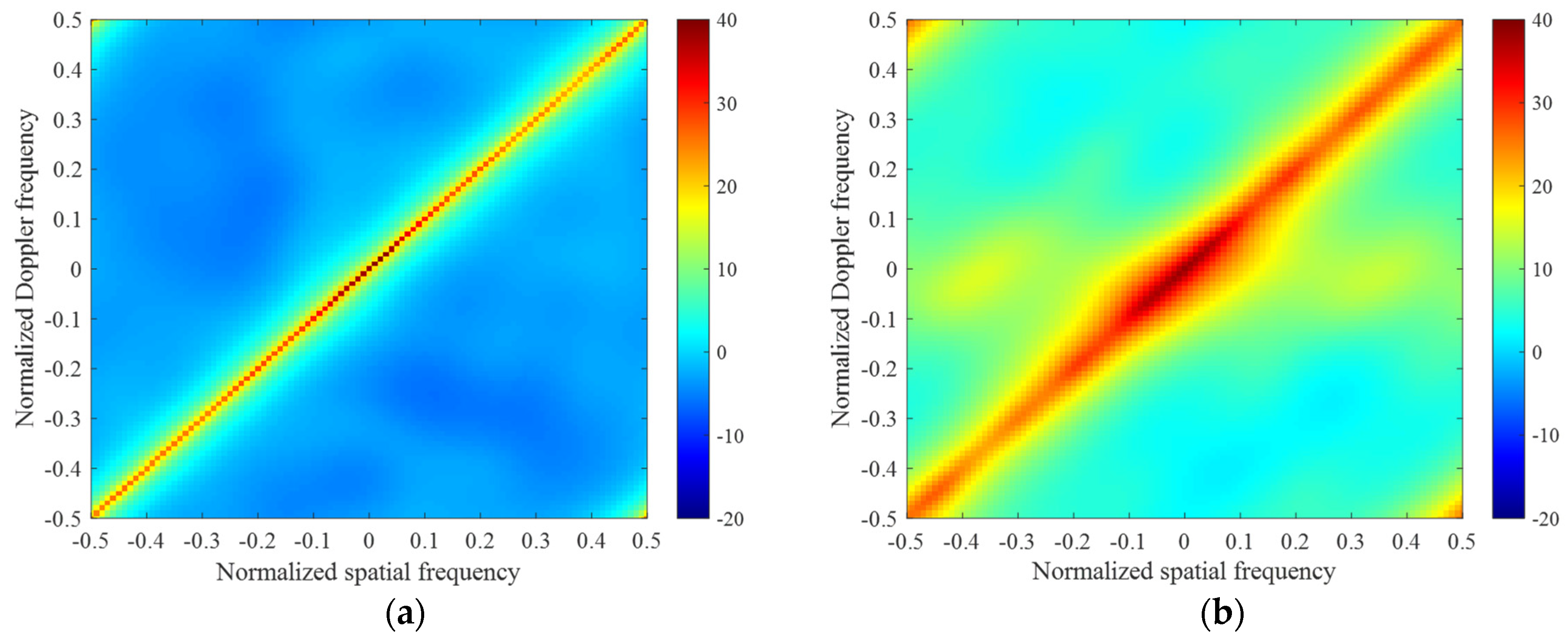
- We combine the IAA spectrum method with the weighted norm method, and a fast IAA–based SR–STAP method is proposed. Compared with the STAP method, which directly uses the IAA method, the proposed method can estimate the CNCM more accurately. Compared with the weighted norm method, the proposed method has an analytical solution.
- (2)
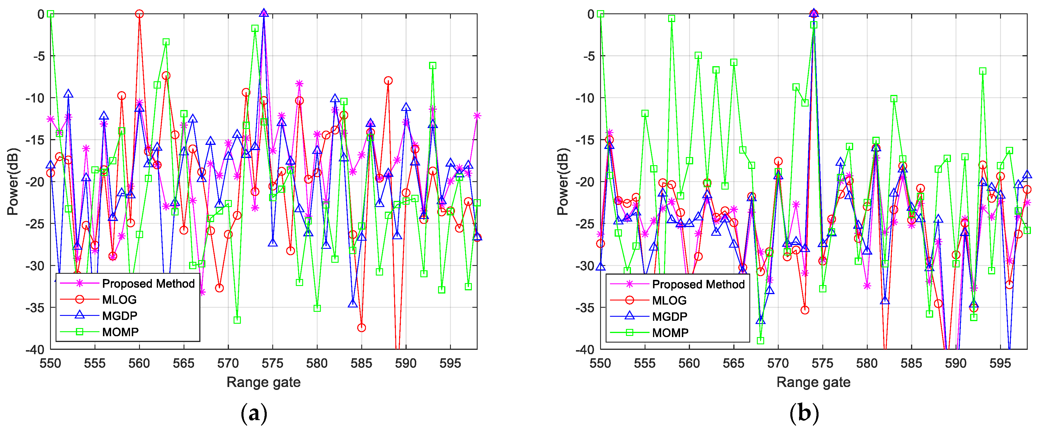
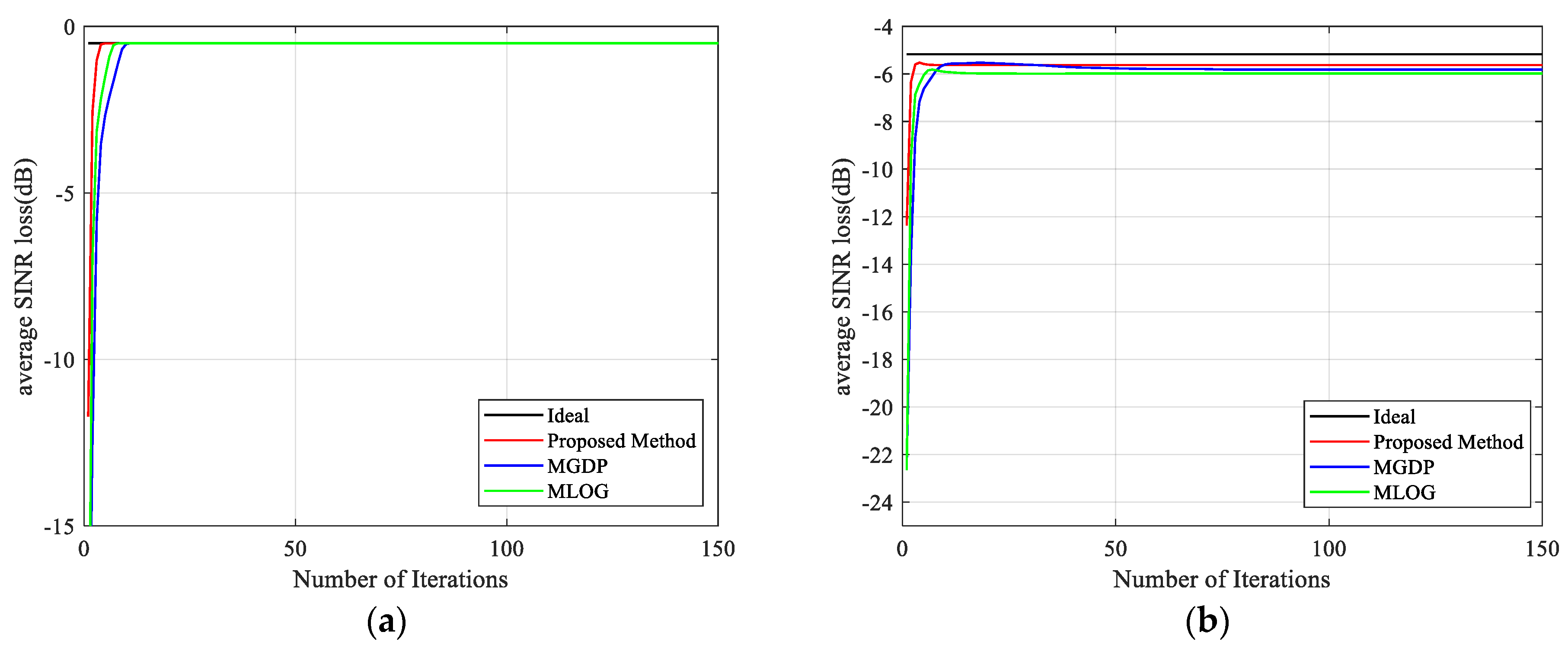
- The proposed method has fast convergence performance, a shorter running time, and good clutter suppression performance.
- (3)
- Through a comparison with other STAP methods, simulation results and a performance analysis are given to demonstrate the effectiveness of the proposed method.
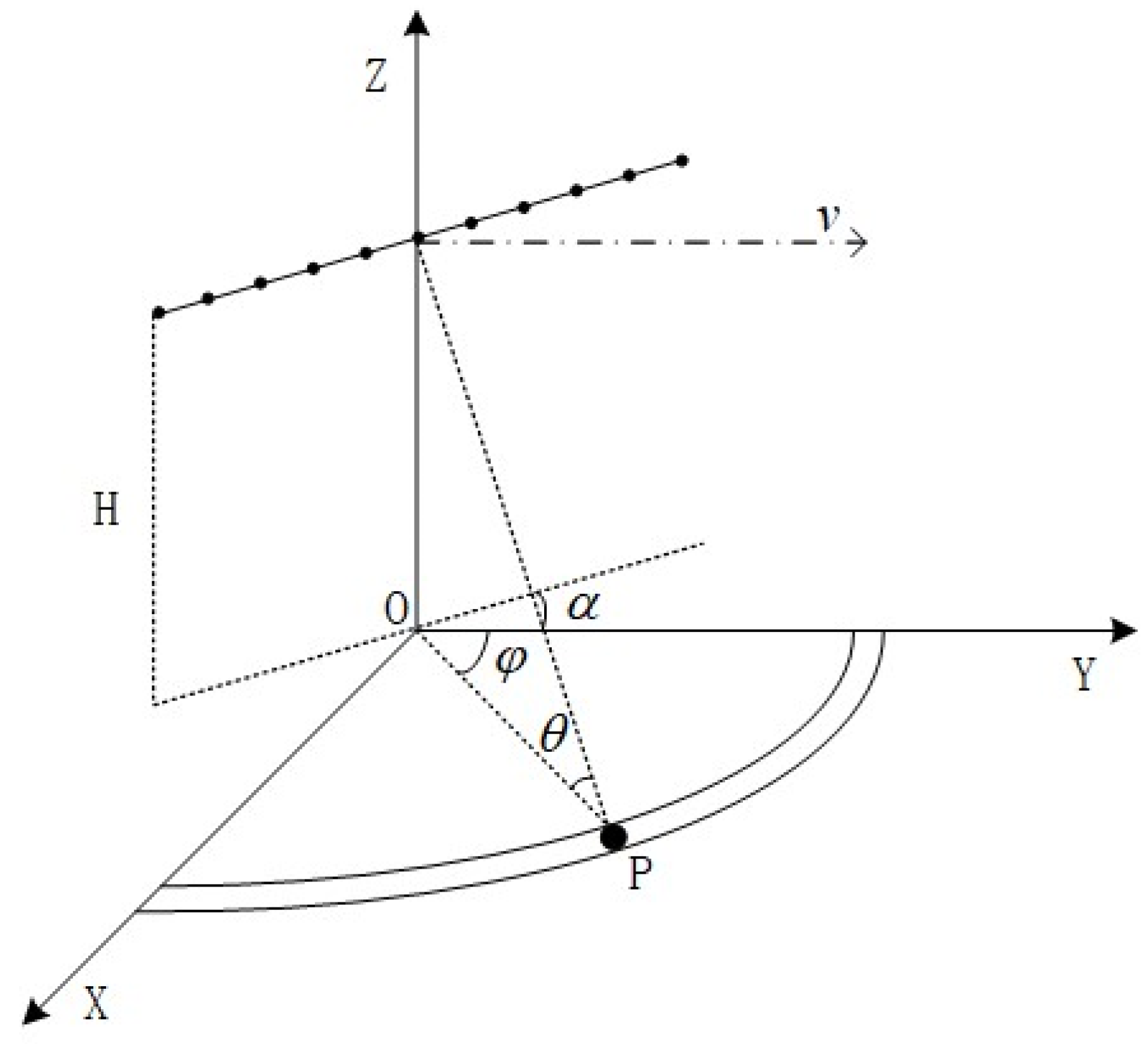
2. Signal Model and Problem Formulation
2.1. Signal Model
2.2. Review of IAA
2.3. Proposed Method
3. Performance Assessment
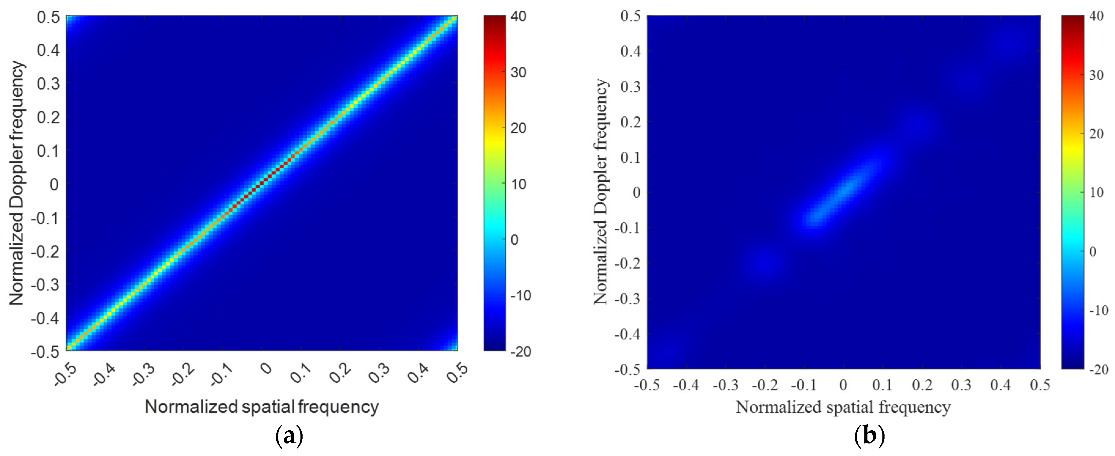
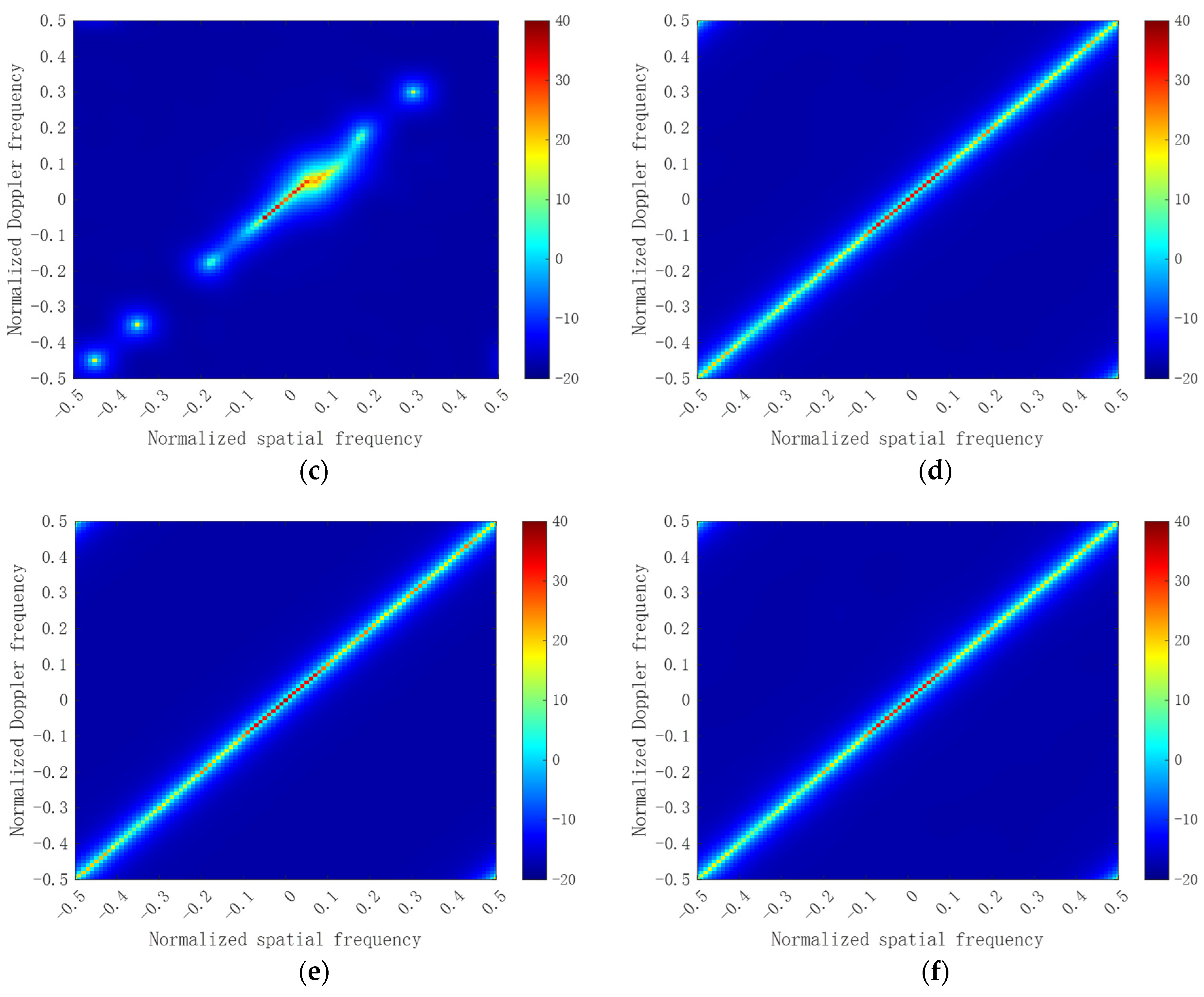
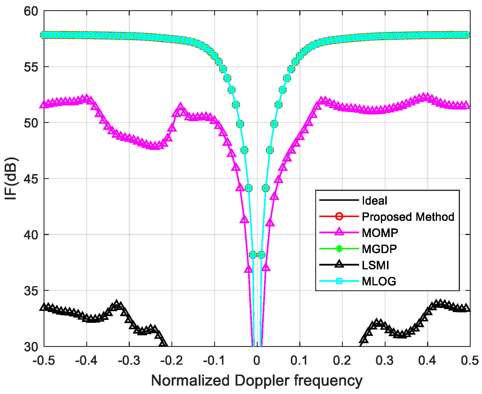
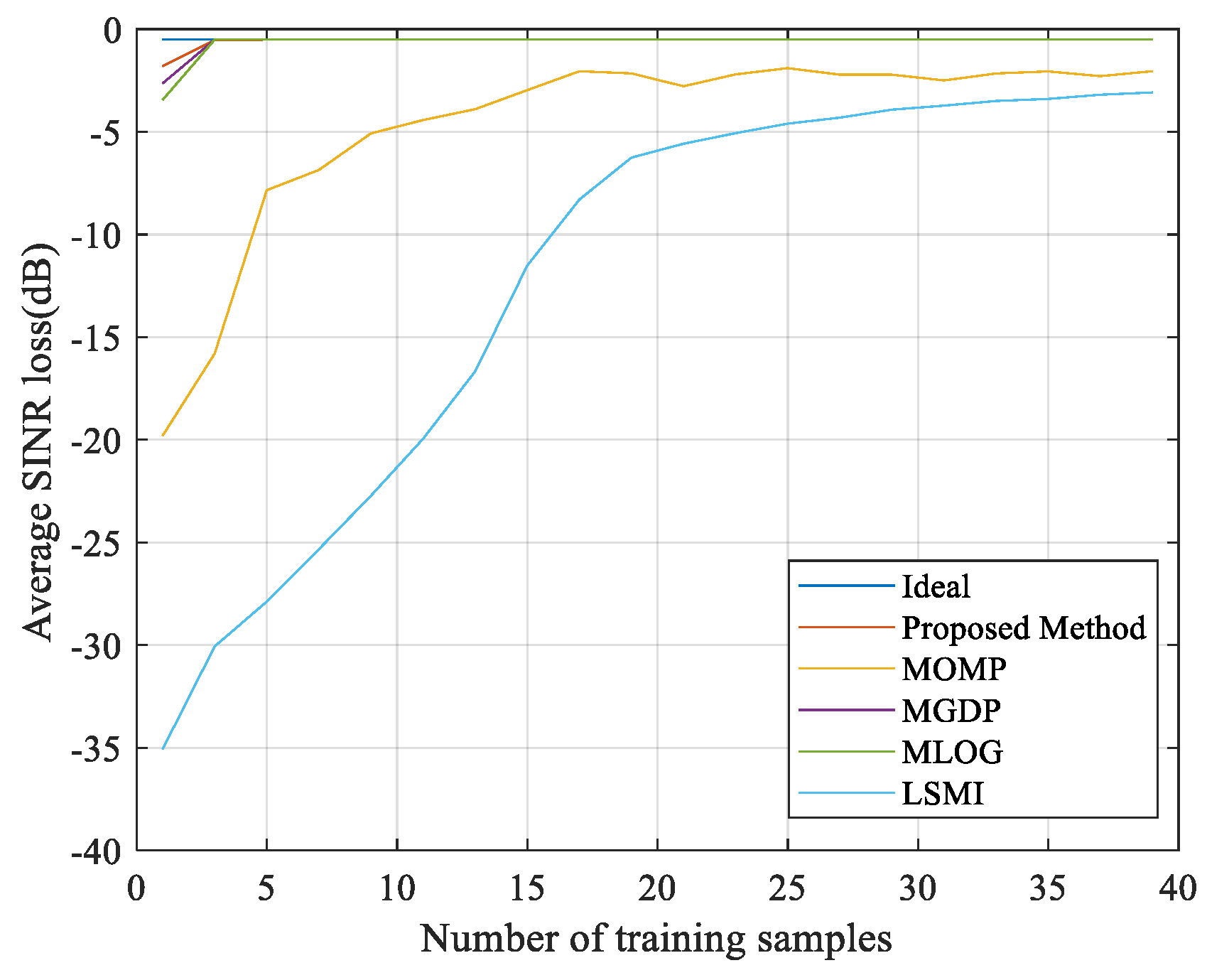
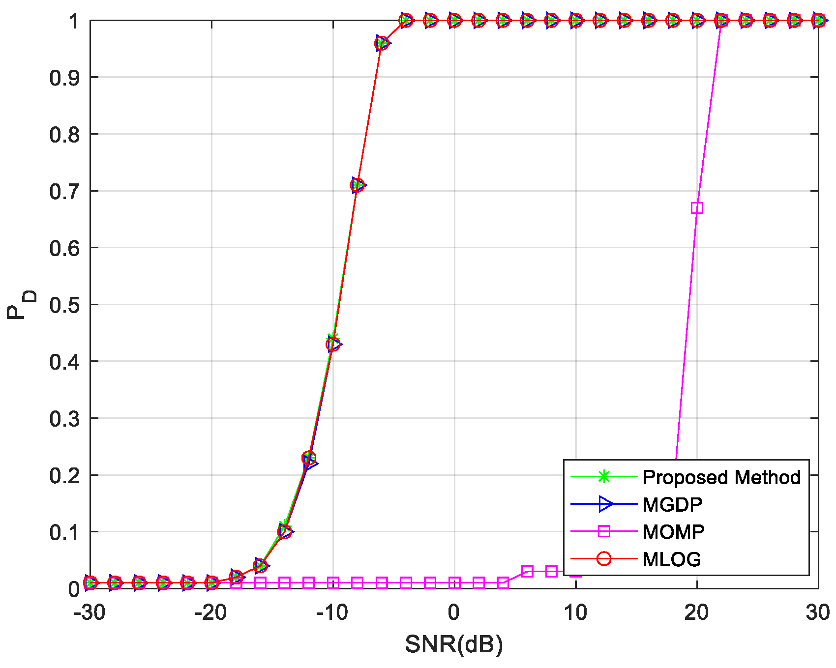
3.1. Ideal Case
3.2. Non–Ideal Case
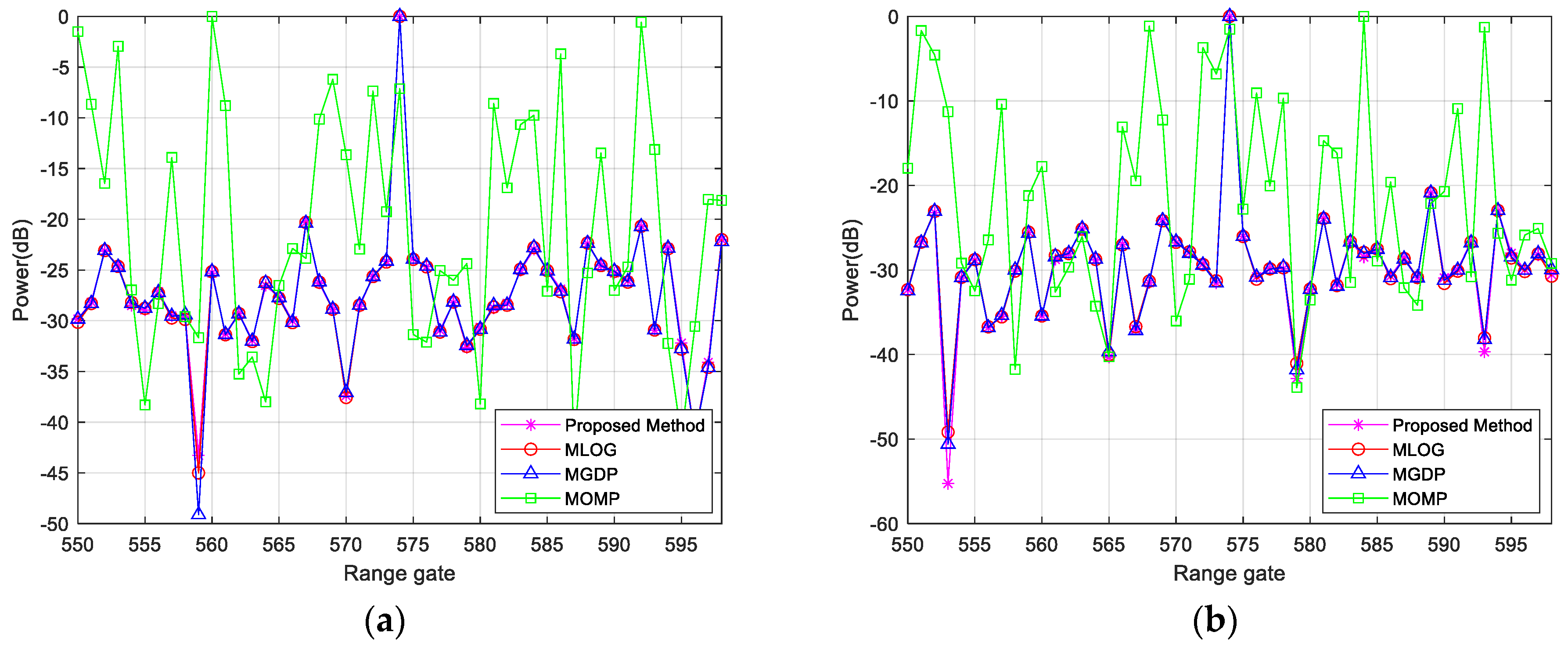
3.3. Measured Data
4. Discussion
5. Conclusions
Author Contributions
Funding
Data Availability Statement
Conflicts of Interest
References
- Ward, J. Space–Time Adaptive Processing for Airborne Radar; Lincoln Laboratory: Lexington, MA, USA, 1998. [Google Scholar]
- Brennan, L.E.; Reed, I.S. Theory of adaptive radar. IEEE Trans. Aerosp. Electron. Syst. 1973, 9, 237–252. [Google Scholar] [CrossRef]
- Sedwick, R.J.; Hacker, T.L.; Marais, K. Performance analysis for an interferometric space–based GMTI system. In Proceedings of the Record of the IEEE 2000 International Radar Conference [Cat. No. 00CH37037], Alexandria, VA, USA, 12 May 2000; pp. 689–694. [Google Scholar]
- Maher, J.; Callahan, M.; Lynch, D. Effects of clutter modeling in evaluating STAP processing for space–based radars. In Proceedings of the Record of the IEEE 2000 International Radar Conference [Cat. No. 00CH37037], Alexandria, VA, USA, 12 May 2000; pp. 565–570. [Google Scholar]
- Devaney, A.J. Time reversal imaging of obscured targets from multistatic data. IEEE Trans. Antennas Propag. 2005, 53, 1600–1610. [Google Scholar] [CrossRef]
- Ciuonzo, D. On time–reversal imaging by statistical testing. IEEE Signal Process. Lett. 2017, 24, 1024–1028. [Google Scholar] [CrossRef]
- Goldstern, J.S.; Reed, I.S.; Zulch, P.A. Multistage partially adaptive STAP CFAR detection algorithm. IEEE Trans. Aerosp. Electron. Syst. 1999, 35, 645–661. [Google Scholar] [CrossRef]
- Tong, Y.L.; Wang, T.; Wu, J.X. Improving EFA–STAP performance using persymmetric covariance matrix estimation. IEEE Trans. Aerosp. Electron. Syst. 2015, 51, 924–936. [Google Scholar] [CrossRef]
- Goldstein, J.S.; Reed, I.S. Reduced rank adaptive filtering. IEEE Trans. Signal Process. 1997, 45, 493–496. [Google Scholar] [CrossRef]
- Zhang, W.; He, Z.S.; Li, H.Y.; Li, J.; Duan, X. Beam–space reduced–dimension space–time adaptive processing for airborne radar in sample starved heterogeneous environments. IET Radar Sonar Navig. 2016, 10, 1627–1634. [Google Scholar]
- Sarkar, T.K.; Wang, H.; Park, S.; Adve, R.; Koh, J.; Kim, K.; Zhang, Y.; Wicks, M.C.; Brown, R.D. A deterministic least squares approach to space time adaptive processing (STAP). IEEE Trans. Aerosp. Electron. Syst. 2001, 49, 91–103. [Google Scholar]
- Cristallini, D.; Burger, W. A Robust Direct Data Domain Approach for STAP. IEEE Trans. Signal Process. 2012, 60, 1283–1294. [Google Scholar] [CrossRef]
- Melvin, W.L.; Showman, G.A. An approach to knowledge–aided covariance estimation. IEEE Trans. Aerosp. Electron. Syst. 2006, 42, 1021–1042. [Google Scholar] [CrossRef]
- Stoica, P.; Li, J.; Zhu, X. On Using a priori Knowledge in Space–Time Adaptive Processing. IEEE Trans. Signal. Process. 2008, 56, 2598–2602. [Google Scholar] [CrossRef]
- Mallet, S.; Zhang, Z. Matching pursuits with time frequency dictionaries. IEEE Trans. Signal Process. 1993, 41, 3397–3415. [Google Scholar] [CrossRef]
- Pati, Y.C.; Rezaiifar, R.; Krishnaprasad, P.S. Orthogonal matching pursuit: Recursive function approximation with applications to wavelet decomposition. In Proceedings of the 27th Asilomar Conference on Signal, Systems and Computers, Pacific Grove, CA, USA, 1–3 November 1993; pp. 40–44. [Google Scholar]
- Candes, E.; Wakin, M.; Boyd, S. Enhancing sparsity by reweighted minimization. J. Fourier Anal. Appl. 2008, 14, 877–905. [Google Scholar] [CrossRef]
- Chartrand, R.; Yin, W. Iteratively reweighted algorithms for compressive sensing. In Proceedings of the 2008 IEEE International Conference on Acoustics, Speech and Signal Processing, Las Vegas, NV, USA, 31 March–4 April 2008; pp. 3869–3872. [Google Scholar]
- Xu, X.; Wei, X.H.; Ye, Z.F. DOA estimation based on sparse signal recovery utilizing weighted penalty. IEEE Signal Process. Lett. 2012, 19, 155–158. [Google Scholar] [CrossRef]
- Tipping, M.E. Spars Bayesian learning and the relevance vector machine. J. Math. Learn. 2001, 1, 211–244. [Google Scholar]
- Wipf, D.P.; Rao, B.D. An empirical Bayesian strategy for solving the simultaneous sparse approximation problem. IEEE Trans. Signal Process. 2007, 55, 3704–3716. [Google Scholar] [CrossRef]
- Duan, K.Q.; Wang, Z.T.; Xie, W.C.; Chen, H.; Wang, Y.L. Sparsity–based STAP algorithm with multiple measurement vectors via sparse Bayesian learning strategy for airborne radar. IET Signal Process. 2017, 11, 544–553. [Google Scholar] [CrossRef]
- Wang, Q.; Yu, H.; Li, J. Sparse Bayesian Learning Using Generalized Double Pareto Prior for DOA Estimation. IEEE Signal Process. Lett. 2021, 28, 1744–1748. [Google Scholar] [CrossRef]
- Zhang, S.; Wang, T.; Liu, C.; Wang, D. A Space–Time Adaptive Processing Method Based on Sparse Bayesian Learning for Maneuvering Airborne Radar. Sensors 2022, 22, 5479. [Google Scholar] [CrossRef] [PubMed]
- Yang, Z.C.; Li, X.; Wang, H.; Jiang, W. Adaptive clutter suppression based on iterative adaptive approach for airborne radar. Signal Process. 2013, 93, 3567–3577. [Google Scholar] [CrossRef]
- Fang, J.; Wang, F.Y.; Shen, Y.N.; Li, H.B.; Rick, S.B. Super–resolution compressed sensing for line spectral estimation: An iterative reweighted approach. IEEE Trans. Signal Process. 2016, 64, 4649–4662. [Google Scholar] [CrossRef]
- Bandiera, F.; Miao, A.D.; Riccie, G. Adaptive CFAR radar detection with conic rejection. IEEE Trans. Signal Process. 2007, 55, 2533–2541. [Google Scholar] [CrossRef]
- Liu, W.J.; Liu, J.; Hao, C.P.; Gao, Y.C.; Wang, Y.L. Multichannel adaptive signal detection: Basic theory and literature review. Sci. China Inf. Sci. 2022, 65, 121301. [Google Scholar] [CrossRef]


| Acronyms | Full Name |
|---|---|
| AEW | Airborne early warning |
| CNCM | Clutter plus noise covariance matrix |
| CUT | Cell under test |
| DDD | Direct data domain |
| IAA | Iterative adaptive approach |
| IID | Independent and identically distributed |
| KA | Knowledge–aided |
| SBL | Sparse Bayesian learning |
| STAP | Space–time adaptive processing |
| Step 1 | Input data and dictionary matrix |
| Step 2 | Initialize and |
| Step 3 | Calculate using (29) |
| Step 4 | Calculate using (34) |
| Step 5 | Calculate using (33) |
| Step 6 | Calculate using (35) |
| Step7 | Repeat step 3, step 4, step 5, and step 6 until a stopping criterion is satisfied |
| Step 8 | Calculate CNCM |
| Step 9 | Compute STAP weight |
| Parameter | Value |
|---|---|
| Number of elements in array | 8 |
| Number of pulses per CPI | 8 |
| Pulse repetition frequency | 2000 Hz |
| Receiver bandwidth | 2.5 MHz |
| Platform height | 9000 m |
| Wavelength | 0.3 m |
| Platform velocity | 150 m/s |
| Clutter–to noise ratio | 40 dB |
| Operation frequency | 1 Ghz |
| Algorithm | Average Running Time (s) |
|---|---|
| M–OMP | 0.03 |
| M–GDP | 7.26 |
| M–LOG | 0.45 |
| Proposed Method | 0.22 |
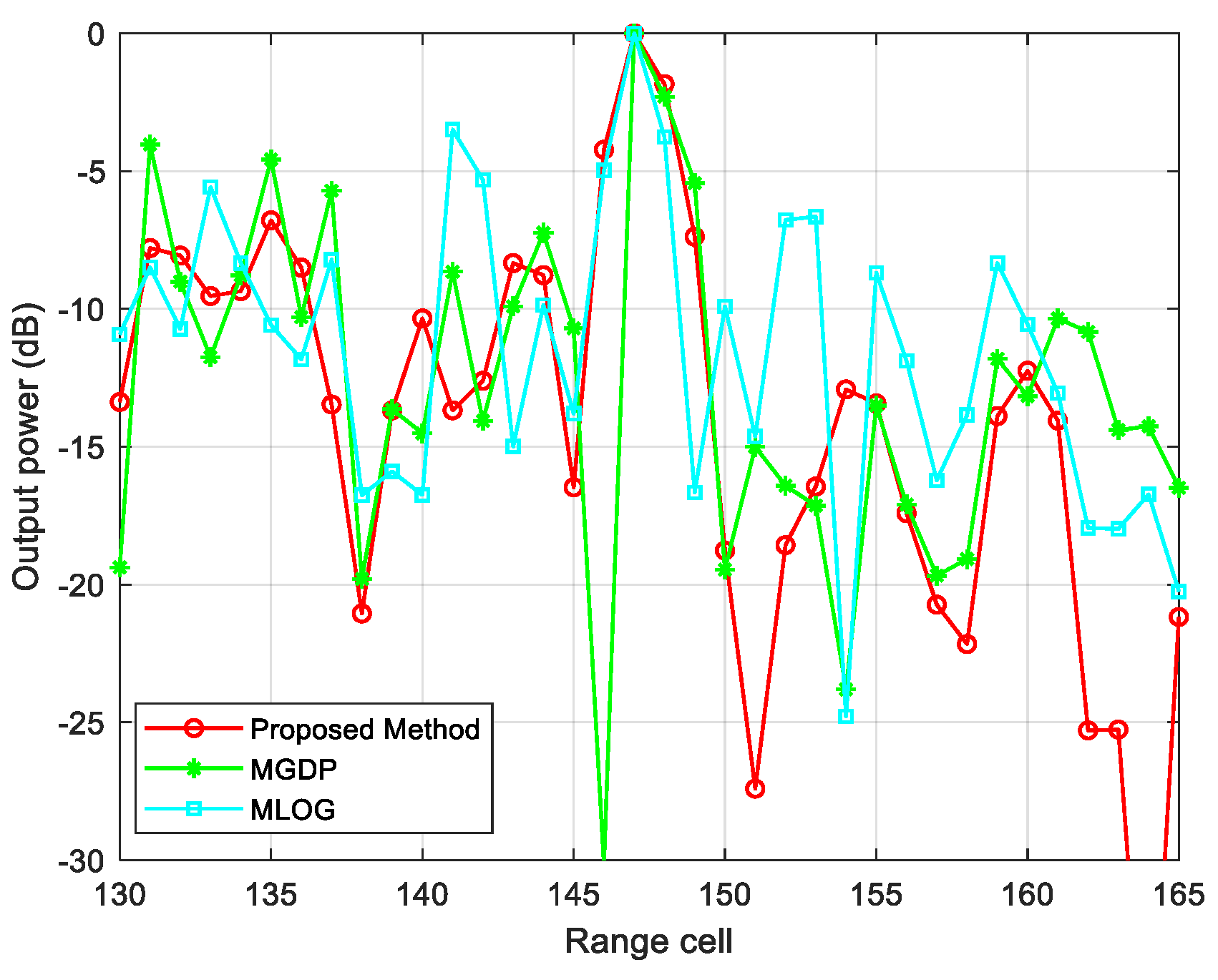
| Algorithm | Power (dB) |
|---|---|
| Proposed Method | −12.0662 |
| M–GDP | −10.5169 |
| M–LOG | −10.1075 |
Disclaimer/Publisher’s Note: The statements, opinions and data contained in all publications are solely those of the individual author(s) and contributor(s) and not of MDPI and/or the editor(s). MDPI and/or the editor(s) disclaim responsibility for any injury to people or property resulting from any ideas, methods, instructions or products referred to in the content. |
© 2024 by the authors. Licensee MDPI, Basel, Switzerland. This article is an open access article distributed under the terms and conditions of the Creative Commons Attribution (CC BY) license (https://creativecommons.org/licenses/by/4.0/).
Share and Cite
Zhang, S.; Wang, T.; Liu, C.; Ren, B. A Fast IAA–Based SR–STAP Method for Airborne Radar. Remote Sens. 2024, 16, 1388. https://doi.org/10.3390/rs16081388
Zhang S, Wang T, Liu C, Ren B. A Fast IAA–Based SR–STAP Method for Airborne Radar. Remote Sensing. 2024; 16(8):1388. https://doi.org/10.3390/rs16081388
Chicago/Turabian StyleZhang, Shuguang, Tong Wang, Cheng Liu, and Bing Ren. 2024. "A Fast IAA–Based SR–STAP Method for Airborne Radar" Remote Sensing 16, no. 8: 1388. https://doi.org/10.3390/rs16081388
APA StyleZhang, S., Wang, T., Liu, C., & Ren, B. (2024). A Fast IAA–Based SR–STAP Method for Airborne Radar. Remote Sensing, 16(8), 1388. https://doi.org/10.3390/rs16081388