Spatial Downscaling of ESA CCI Soil Moisture Data Based on Deep Learning with an Attention Mechanism

Abstract

Soil moisture (SM) is a critical variable affecting ecosystem carbon and water cycles and their feedback to climate change. In this study, we proposed a convolutional neural network (CNN) model embedded with a residual block and attention module, named SMNet, to spatially downscale the European Space Agency (ESA) Climate Change Initiative (CCI) SM product. In the SMNet model, a lightweight Convolutional Block Attention Module (CBAM) dual-attention mechanism was integrated to comprehensively extract the spatial and channel information from the high-resolution input remote sensing products, the reanalysis meteorological dataset, and the topographic data. The model was employed to downscale the ESA CCI SM from its original spatial resolution of 25 km to 1 km in California, USA, in the annual growing season (1 May to 30 September) from 2003 to 2021. The original ESA CCI SM data and in situ SM measurements (0–5 cm depth) from the International Soil Moisture Network were used to validate the model’s performance. The results show that compared with the original ESA CCI SM data, the downscaled SM data have comparable accuracy with a mean correlation (R) and root mean square error (RMSE) of 0.82 and 0.052 m³/m³, respectively. Moreover, the model generates reasonable spatiotemporal SM patterns with higher accuracy in the western region and relatively lower accuracy in the eastern Nevada mountainous area. In situ site validation results in the SCAN, the SNOTEL network, and the USCRN reveal that the R and RMSE are 0.62, 0.63, and 0.77, and 0.077 m³/m³, 0.093 m³/m³, and 0.078 m³/m³, respectively. The results are slightly lower than the validation results from the original ESA CCI SM data. Overall, the validation results suggest that the SMNet downscaling model proposed in this study has satisfactory performance in handling the task of soil moisture downscaling. The downscaled SM model not only preserves a high level of spatial consistency with the original ESA CCI SM model but also offers more intricate spatial variations in SM depending on the spatial resolution of model input data.

1. Introduction

Soil moisture (SM) is crucial for controlling global water and carbon cycles, affecting ecosystem feedback to extreme climate events, and providing information about water resource management [1], because most water that is not lost by evapotranspiration or runoff is stored in the soil. Moreover, SM controls the land surface energy balance and influences surface albedo [2]. High-spatial resolution SM data have been increasingly in demand for regional applications [3], particularly for the surveillance of extreme climatic events such as droughts and floods [4,5,6], agricultural irrigation [7,8], weather forecasting [9], and wildfire prediction. Therefore, it is necessary to produce and provide accurate SM data with high spatial resolution to meet those requirements.

Traditional SM data are collected by in situ measurements. Although in situ observation stations can monitor SM changes at different soil layers with high accuracy, they are limited in both time and space [10]. With the advancement of land surface models and remote sensing (RS) technology, continuous SM data in spatial and temporal dimensions have been obtained from RS and model simulations [11]. In comparison with land surface models which have large differences in the accuracy of simulated SM data because of the model structures and parameterizations [12], RS is able to directly estimate the spatial and temporal variations of SM at the regional and global scales according to the relationship between the electromagnetic spectrum and the top centimeters of soil water content. At present, RS SM data have been mainly derived from optimal RS, microwave RS, and thermal infrared sensors [13]. Among them, microwave (active and passive) RS has exceptional potential in SM retrieval, owing to its advantages of all-day and all-weather multi-polarization, and high penetrability and sensitivity to SM [14]. Since the 1970s, an array of active and passive RS satellites and sensors, e.g., the Advanced Microwave Scanning Radiometer (AMSR) and the SM and Ocean Salinity (SMOS) and Soil Moisture Active Passive (SMAP) satellites, have been deployed for the observation of SM variations [15,16,17,18,19], providing greater convenience in obtaining dynamic SM information at various spatiotemporal resolutions over large regions [20]. However, the majority of SM products from microwave RS are usually provided with relatively coarse spatial resolution (10~50 km), which cannot meet the practical needs of regional, hydrological, and agricultural applications.

In order to acquire SM data with high or super-high spatial resolution, numerous spatial downscaling approaches have been developed in recent years [21,22,23], including RS data fusion, statistical regression models, data assimilation, and machine learning (ML) methods. Considering the advantage of high-spatial resolution in active microwave RS and high sensitivity to SM in passive microwave RS, merging active and passive microwave SM products is a common method for SM downscaling [24,25]. However, some drawbacks of this method cannot be ignored, such as the asynchronous observations of active and passive microwave RS [26]. In comparison, optical and thermal RS provide higher spatial and temporal observations on surface variables, and how to combine optical (or thermal) and microwave RS to enhance the spatial resolution of RS SM data has received more attention [27,28]. Zhu et al. [29] applied apparent thermal inertia data from MODIS products to downscale the European Space Agency (ESA) Climate Change Initiative (CCI) SM data at 1 km resolution and demonstrated the accuracy of downscaled ESA CCI SM data, which reached 0.552. Zhao et al. [30] proposed a seamless downscaling method for ESA CCI SM data based on MODIS daily land surface temperature (LST) and normalized difference vegetation index (NDVI) products and reported that this method could generate high-resolution SM data without spatiotemporal gaps. In addition, statistical regression models and data assimilation methods are often used to downscale SM data. For example, Song et al. [31] utilized geographically weighted regressions to establish the relationship between AMSR-2 SM data and MODIS LST and NDVI data and implement the downscaling process. Kolassa et al. [32] used an ensemble Kalman filter to assimilate the daily SM data retrieved from microwave RS (i.e., AMSR-E brightness temperature and ASCAT backscatter) into the NASA catchment land surface model and revealed that a data assimilation system could yield a higher-quality SM product. Nonetheless, the lack of universality of statistical models and the complexity of parameterization of land surface models make them difficult to apply more generally.

ML has been widely adopted to generate high-resolution SM data, owing to its good performance in handling non-linear problems [26]. Hu et al. [33] utilized random forest (RF) to establish the relationship between the SMAP SM and input surface variables and demonstrated that the downscaled SMAP SM data could capture the spatial heterogeneity and dynamic changes in SM. Wei et al. [34] proposed an SMAP SM downscaling method based on a gradient boosting decision tree (GBDT) algorithm over the entire Tibetan Plateau and reported that the method could preserve SMAP SM accuracy. Additionally, numerous investigations have compared the performance of different ML methods in RS SM downscaling. Liu et al. [35] evaluated the performance of artificial neural network (ANN), K nearest neighbor (KNN), Bayesian (BAYE), random forest (RF), classification and regression tree (CART), and support vector machine (SVM) methods in ESA CCI SM downscaling and showed that the RF algorithm could significantly improve the spatial resolution of ESA CCI SM data compared to ANN, BAYE, CART, KNN, and SVM methods.

Unlike the abovementioned ML methods, deep learning (DL) can automatically study higher-level and deeper features from input data, which is more suitable for dealing with complex non-linear relationships. Zhao et al. [36] compared the performances of backpropagation neural network, RF, and three DL methods in downscaling SMAP SM data of the Tibetan Plateau and revealed that the DL methods had a more superior ability to provide more spatial patterns and texture details in complex surfaces. Jiang et al. [37] introduced a novel deep residual cycle GAN-based fusion method, treating HR data as spectral features, to effectively downscale SMAP SM data from 36 km to 9 km. And the results demonstrated that this method achieved commendable performance on two distinct scales of test datasets. In recent years, attention mechanisms have gained remarkable prominence within the realm of DL models, concurrently catalyzing advancements in research and applications within the domain of RS. For instance, Sit et al. [38] employed a graph convolutional network with spatiotemporal attention mechanisms to spatially downscale streamflow data, significantly enhancing DL’s role in flood forecasting. Additionally, researchers like G. Liu et al. [39] introduced a DL model incorporating a terrain-guided attention mechanism, establishing non-linear mapping for downscaling the temperature distribution in the southwestern region of China. Nevertheless, the exploration of attention mechanism-based DL methods for SM downscaling remains an unexplored frontier.

In this study, we developed a downscaling model of ESA CCI SM data based on a DL method with a dual-attention mechanism (named SMNet model) by employing the RS, meteorological, topographic, and in situ measurements. And this study was conducted in the state of California in the USA, which has large spatial heterogeneity in SM owing to its diverse terrains and complex hydroclimate. The specific objectives were (1) to establish an SM downscaling model by considering a convolutional neural network (CNN) and a dual-attention mechanism, (2) to conduct a thorough performance evaluation of the SMNet model using both original ESA CCI SM data and in situ SM measurements, and (3) to explore the potential ability of the SMNet model for spatial and temporal extrapolation in ESA CCI SM data.

2. Materials and Methods

2.1. Study Area and Data

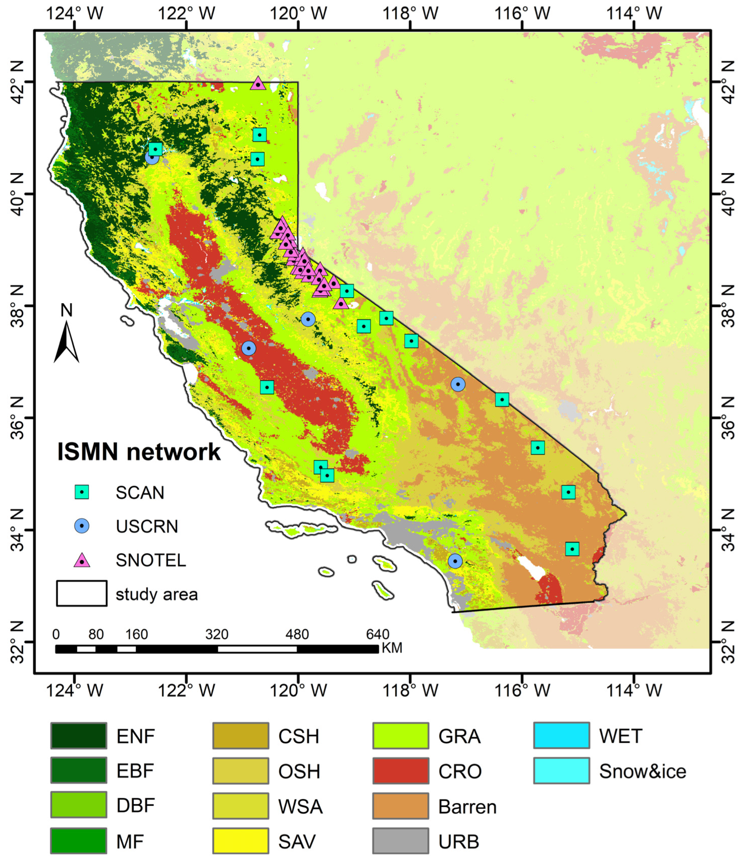
2.1.1. Study Area

The study area covers the entire state of California, which is located in the southwestern part of the continental United States, with a total area of approximately 423,970 km² (Figure 1). California has varied topography and diverse ecosystems, leading to high spatial heterogeneity in SM. Its central part is the Central Valley, which is the most productive agricultural region in the United States. In the west coast, northern, and eastern areas of California, there are some mountains with large areas of forests. In addition, shrubland and deserts with sparse vegetation occupy most portions of southeastern California. The prevailing climate of California is the Mediterranean climate, with a dry summer and a wet winter. Inland, the climate is more continental, and the southeastern regions of California are dominated by the desert climate. Influenced by different climates, the precipitation of California ranges from more than 2500 mm per year in the northwest forest to traces in the southeastern desert. Warmer and drier summers and climate changes make California prone to drought and wildfires. In recent decades, California has experienced more severe and frequent droughts and wildfires (e.g., the 2012–2016 California drought and the 2020 wildfires), which significantly influence local human activities and agricultural production. Given the complexity of hydroclimate patterns and the escalating climate variability in the region, generating high-resolution SM data holds significant importance for effective water resource management and wildfire prevention in California.

2.1.2. ESA CCI SM Dataset

ESA CCI SM data are produced by the European Space Agency’s (ESA) program on Global Monitoring of Essential Climate Variables (ECV) (known as the Climate Change Initiative, CCI), which is aimed to create a complete and consistent global SM dataset [40]. These SM data merge various SM products from multiple active and passive microwave RS sensors into harmonized data records by synergistically combing the strengths of the individual products [41]. ESA CCI SM data provide three products, i.e., (1) the active-microwave-based-only product (ACTIVE), (2) the passive-microwave-based-only product (PASSIVE), and (3) the combined active–passive product (COMBINED) [17]. In this study, the COMBINED product from ESA CCI SM version 07.1 (https://data.ceda.ac.uk/neodc/esacci/soil_moisture/data/daily_files/COMBINED/v07.1, accessed on 10 May 2022) [41] was used for spatial downscaling. The SM data estimate the water volume in the surface soil layer (approximately top 5 cm), and are available at a temporal resolution of one day and a spatial resolution of 25 km on the World Geodetic System 1984 (WGS-84) reference system, covering the period from 2003 to 2021.

2.1.3. MODIS Products

The high-resolution surface reflectance data from MODIS (MCD43A4) were used for ESA CCI SM downscaling. The MCD43A4 data (https://www.earthdata.nasa.gov/eosdis, accessed on 10 May 2022) provide bidirectional reflectance distribution function (BRDF)-adjusted reflectance with a resolution of 500 m/daily. Based on the surface reflectance data, several vegetation indices (e.g., NDVI, enhanced vegetation index (EVI), near-infrared vegetation index (NIRv), and kernel NDVI (kNDVI)) were additionally calculated by combining the different surface reflectance bands.

$$\mathrm{N}\mathrm{D}\mathrm{V}\mathrm{I}=\frac{{\mathsf{\rho }}_{\mathrm{N}\mathrm{I}\mathrm{R}}-{\mathsf{\rho }}_{\mathrm{R}\mathrm{E}\mathrm{D}}}{{\mathsf{\rho }}_{\mathrm{N}\mathrm{I}\mathrm{R}}+{\mathsf{\rho }}_{\mathrm{R}\mathrm{E}\mathrm{D}}}$$

(1)

$$\mathrm{E}\mathrm{V}\mathrm{I}=\mathrm{G}·\frac{{\mathsf{\rho }}_{\mathrm{N}\mathrm{I}\mathrm{R}}-{\mathsf{\rho }}_{\mathrm{R}\mathrm{E}\mathrm{D}}}{{\mathsf{\rho }}_{\mathrm{N}\mathrm{I}\mathrm{R}}+{\mathrm{C}}_1·{\mathsf{\rho }}_{\mathrm{R}\mathrm{E}\mathrm{D}}-{\mathrm{C}}_2·{\mathsf{\rho }}_{\mathrm{B}\mathrm{L}\mathrm{U}\mathrm{E}}+\mathrm{L}}$$

(2)

$$\mathrm{N}\mathrm{I}{\mathrm{R}}_{\mathrm{v}}={\mathsf{\rho }}_{\mathrm{N}\mathrm{I}\mathrm{R}}·\mathrm{N}\mathrm{D}\mathrm{V}\mathrm{I}$$

(3)

$$\mathrm{k}\mathrm{N}\mathrm{D}\mathrm{V}\mathrm{I}=\tanh \left({\mathrm{N}\mathrm{V}\mathrm{D}\mathrm{I}}^2\right)$$

(4)

where ${\mathsf{\rho }}_{\mathrm{N}\mathrm{I}\mathrm{R}}$ is the near-infrared band, ${\mathsf{\rho }}_{\mathrm{R}\mathrm{E}\mathrm{D}}$ is the red band, and ${\mathsf{\rho }}_{\mathrm{B}\mathrm{L}\mathrm{U}\mathrm{E}}$ is the blue band [42]. $\mathrm{L}$, ${\mathrm{C}}_1$, ${\mathrm{C}}_2$, and $\mathrm{G}$ in EVI are 1, 5, 7.5, and 2.5 [43].

The land cover types from MCD12Q1 in California were reclassified into fourteen categories. MOD44W products (version 6) were also selected for land and sea masks [44]. MCD12Q1 has a resolution of 500 m/yearly, and MOD44W has a spatial and temporal resolution of 250 m/yearly. All of them were used as auxiliary input data for the SM downscaling model.

2.1.4. Other Auxiliary Datasets

Precipitation directly drives the spatiotemporal variation of SM [45]. Here, precipitation data were downloaded from Climate Hazards Group InfraRed Precipitation with Station data (CHIRPS). CHIRPS is a quasi-global (50°S–50°N) precipitation product that incorporates in situ observations, satellite-based estimates, and global precipitation climatology. The precipitation data provided by the CHIRPS dataset have a high resolution of 0.05°/daily from 1981 to present [46]. The accuracy of the CHIRPS dataset has been validated in many regions, including Colombia, southwestern North America, and China, and the validation results demonstrate that the CHIRPS dataset is consistent with land surface models and in situ observations in terms of both space and time [46,47,48,49,50]. Here, CHIRPS version 2.0 daily precipitation dataset (Pre) for the period from 2003 to 2021 was used in our study (https://data.chc.ucsb.edu/products/CHIRPS-2.0/, accessed on 22 January 2023).Moreover, considering the legacy effect of precipitation infiltration, we also calculated the precipitation data delayed by one day (Pre.delay) as an input variable impacting SM changes.

Meanwhile, air temperature and soil temperature are considered important factors impacting SM variability, and they were obtained from the ERA5-Land dataset (https://www.ecmwf.int/en/era5-land, accessed on 10 May 2022). The ERA5-Land dataset is developed by the European Centre for Medium-Range Weather Forecasts (ECMWF). This dataset provides hourly information on air temperature, soil temperature, and various land surface variables, boasting a spatial resolution of 0.1°. Here, we calculated the daily mean air temperature and daily mean soil temperature (Tair; Tsoil) based on the hourly data from 2003 to 2021. Similar to precipitation, the air temperature and soil temperature delayed by one day (Tair.delay; Tsoil.delay) were also considered in the downscaled SM model.

Topographic variables play a crucial role in influencing the spatial distribution of SM across various scales [51] and have been incorporated into numerous downscale studies [52,53]. Here, we used the digital elevation model (DEM) data to characterize the topographic conditions in the downscaling model. The DEM data in California was derived from the Shuttle Radar Topography Mission (SRTM) (http://earthexplorer.usgs.gov/, accessed on 10 May 2022) with a spatial resolution of 90 m [54].

2.1.5. In Situ Soil Moisture Measurements

The in situ SM measurements of the International Soil Moisture Measurement Network (ISMN) (https://ismn.earth/en/, accessed on 15 March 2023) were selected as the basis of the model’s accuracy evaluation. We used the in situ data from three networks (SCAN, USCRN, and SNOTEL) during the period of 2019–2021 (1 May to 30 September each year). The positions of the in situ SM stations are depicted in Figure 1.

Table 1. Three networks’ soil moisture in situ information.

Network	SCAN	USCRN	SNOTEL
Latitude	33.65°N–41.05°N	33.44°N–40.65°N	38.07°N–41.98°N
Longitude	122.55°W–115.10°W	123.07°W–117.14°W	120.71°W–119.23°W
Sampling Interval	1 h	1 h	1 h
Depth(cm) Used	0–5	0–5	0–5
Site Used	14	5	28
Time Used	2019–2021	2019–2021	2019–2021

lists the basic information of these three networks, which provide SM measurements at various depths. Considering that the satellite SM products from microwave RS mainly represent SM in the top two to five centimeters of soil [41], and that retrieved SM products based on optical/thermal RS capture only the few millimeters of measurements below the soil surface [55], the in situ SM measurements at a depth of five centimeters were retained for analysis in order to match the measurement depth of remotely sensed SM data by ESA CCI. The temporal resolution of the in situ SM measurements is 1 h, and we averaged these hourly measurements to estimate daily in situ SM measurements (hereafter, “in situ SM” refers to daily in situ SM) to temporally match them with those of the ESA CCI SM. We made the assumption that these sites exhibit spatial homogeneity, and the values assigned to individual sites represent the average values of 1 km pixels.

2.2. Method

Figure 2 shows the procedure and methodology used in this study to downscale ESA CCI SM data. We firstly resampled the high-resolution auxiliary variables during the 2003–2021 period to 25 km and 1 km spatial resolution, with a 1 day timescale. And then, we established the relationship between SM and auxiliary variables at 25 km resolution through model training. Third, the model’s performance was evaluated based on the ESA CCI SM data at 25 km. Finally, after parameter tuning and model evaluation, the model was applied to the 1 km auxiliary data to produce 1 km SM data, and the downscaled SM data were further compared with the original ESA CCI SM data and in situ SM data.

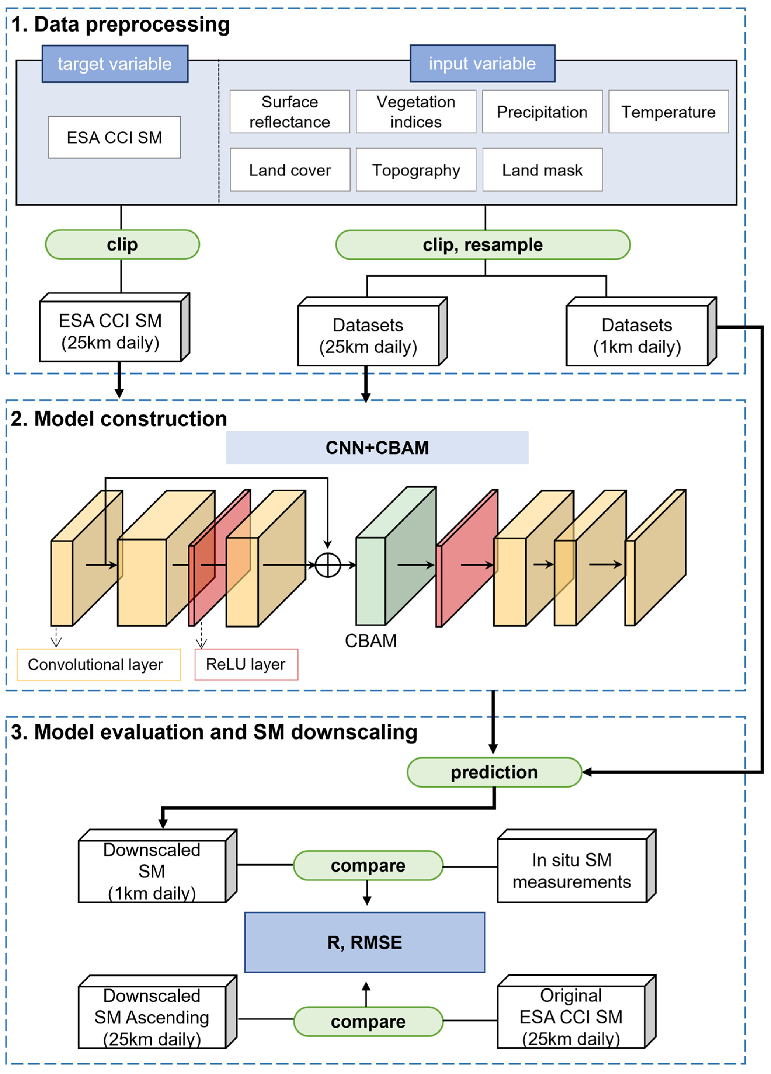
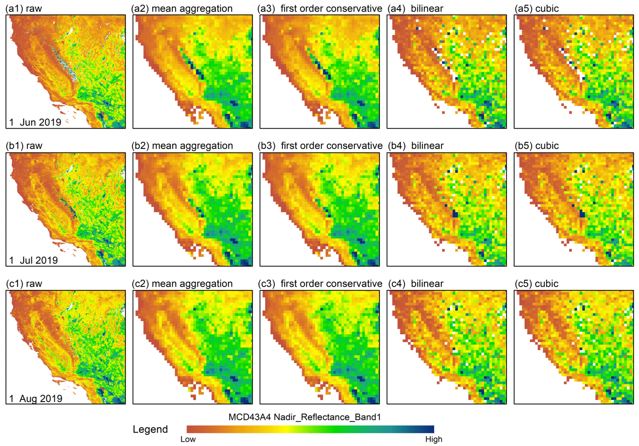
2.2.1. Data Preprocessing

The input data and variables used in the SM downscaled model are listed in

Table 2. The datasets used in this study.

Type of Data	Variable (Notation)		Dataset	Spatial Resolution
Target variable	SM		ESA CCI	25 km
Input variable	Surface reflectance	BLUE, GREEN, RED, NIR, SWIR1, SWIR2, and SWIR3	MCD43A4	500 m
	Vegetation indices	NDVI, EVI, kNDVI, and NIRv	MCD43A4	500 m
	Temperature	Mean air temperature (Tair) and mean air temperature delayed by one day (Tair.delay)	ERA5-Land	0.1°
	Soil temperature	Mean soil temperature (Tsoil) and mean soil temperature delayed by one day (Tsoil.delay)	ERA5-Land	0.1°
	Precipitation	Precipitation (Pre), and precipitation delayed by one day (Pre.delay)	CHIRPS	0.05°
	Land cover	ENF, EBF, DBF, MF, CSH, OSH, WSA, SAV, GRA, CRO, URB, Barren, WET, and Snow&ice	MCD12Q1	500 m
	Topography	DEM	SRTM	90 m
	Land mask		MOD44W	250 m
Validation data	In situ SM	SCAN, USCRN, and SNOTEL	ISMN

, which divides the data into target variable, input variables, and validation data. The diverse input data products are expected to encompass a wide spectrum of SM influencers.

The ESA CCI SM data underwent a quality control procedure prior to constructing the SM downscaling model. SM values with flag values ranging from 1 to 63 or 127 (NAN) were masked to eliminate low-quality SM data. For MCD43A4, we applied the quality index value 0 (best quality only). To ensure high coverage, we interpolated in time for MCD43A4. ERA5-Land data and CHIRPS precipitation data have full spatial and temporal coverage, and therefore, we did not apply any quality filtering on them. All static variables (including land cover, DEM, and land mask) have full coverage on land. All datasets chosen for the SMNet model were reprojected to the WGS-84 coordinate system and clipped to the designated research region.

To match the coarse resolution of the original ESA CCI SM data, all of the auxiliary datasets (MODIS surface reflectance, vegetation indices, temperature, soil temperature, precipitation, DEM, and land mask) were resampled to a 25 km resolution by using a bilinear interpolation method, except for the land cover data, which was resampled by using the majority method. Input variables with different units may affect the accuracy of SM predictions. Thus, data standardization was performed by subtracting the mean and normalizing by the standard deviation, ensuring stability and expediting the training process. If there was a missing value in the SM training sample, all feature values for that pixel were set to zero to prevent the model from learning inaccurate relationships between predictors and the target variable.

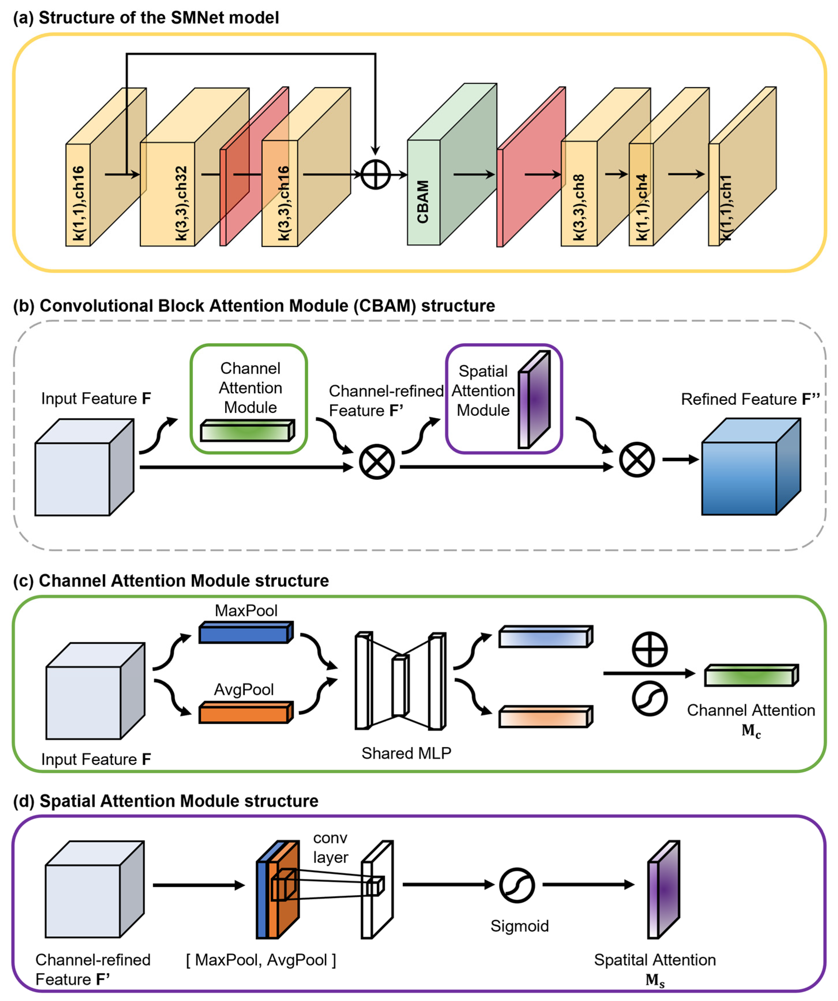
2.2.2. The SMNet Model with a CNN and Attention Mechanism

The framework used in this study is a DL-based downscaling method, called SMNet (Figure 3). The model consists of sequentially arranged convolutional and rectified linear unit (ReLU) layers and a Convolutional Block Attention Module (CBAM). After the first convolutional block, there exists a residual connection skipping one ReLU and two convolutional layers. The CBAM module is embedded in the SMNet model after the first residual block. The convolutional kernels are defined with sizes of either (3,3) or (1,1). This configuration is referenced from the research findings of Gensheimer et al. [42].

We set up the residual block in SMNet to avoid the problems of computing resource consumption and gradient disappearance caused by too many network layers. The Convolutional Block Attention Module (CBAM) was proposed by Woo et al. [56], which is an attention module for the feedforward convolutional neural network, aiming to make up for the problem of the CNN’s locality being too strong and its globality being insufficient. The conceptual diagram and structure of the CBAM include channel and spatial attention. The channel attention module recognizes key image features, while the spatial attention module recognizes key regions [57]. In addition, one of the main advantages of the CBAM is that it is a lightweight module and is able to be inserted on any layer in the neural network to achieve plug-and-play with negligible overhead [58]. The CBAM initially produces the feature map ${\mathrm{F}}^{\prime }$ through the channel attention module, followed by the feature map ${\mathrm{F}}^{″}$ through the spatial attention module, using a middle layer feature map $\mathrm{F}$ as input, as illustrated in Figure 3b. The computational procedure can be represented by Equation (5).

$$\left\{\begin{array}{c}{\mathrm{F}}^{\prime }={\mathrm{M}}_{\mathrm{c}}\left(\mathrm{F}\right)⨂\mathrm{F}\\ {\mathrm{F}}^{″}={\mathrm{M}}_{\mathrm{s}}\left({\mathrm{F}}^{\prime }\right)⨂{\mathrm{F}}^{\prime }\end{array}\right.$$

(5)

where $⨂$ denotes the multiplication operation between corresponding elements. F represents the input feature map. M_c represents the output weight of F′ through the channel attention. M_s represents the output weight of F″ through the spatial attention.

The Integration of the CBAM dual-attention mechanism within our proposed SMNet model is a pivotal advancement which addresses the nuanced challenges posed by diverse and dynamic data sources. The CBAM includes a channel attention module and spatial attention module, and their schematic diagrams are shown in Figure 3c,d.

For the channel attention module, the first step is using the average pooling and maximum pooling operations based on width and height to generate feature maps. Then, the feature maps are fed to the shared MLP layer for summation and activated by the sigmoid function to produce the final channel attention feature weights M_c. The channel attention calculation procedure can be expressed by Equation (6).

$${\mathrm{M}}_{\mathrm{c}}\left(\mathrm{F}\right)=\mathsf{\sigma }\left[\mathrm{M}\mathrm{L}\mathrm{P}\left(\mathrm{A}\mathrm{v}\mathrm{g}\mathrm{P}\mathrm{o}\mathrm{o}\mathrm{l}\left(\mathrm{F}\right)\right)+\mathrm{M}\mathrm{L}\mathrm{P}\left(\mathrm{M}\mathrm{a}\mathrm{x}\mathrm{P}\mathrm{o}\mathrm{o}\mathrm{l}\right(\mathrm{F}\left)\right)\right]$$

(6)

where σ represents the sigmoid function; MLP represents a multi-layer perceptron; AvgPool and MaxPool represent average pooling and maximum pooling.

For the spatial attention module, its input is the channel-refined feature map F′, which is yielded by the average pooling and maximum pooling operations in the channel attention, and is then subject to the concatenate operation. The dimension of the feature map is then reduced using a 7 × 7 convolution kernel, and the sigmoid function is used to generate the spatial attention weights M_s. The spatial attention calculation procedure can be expressed by Equation (7).

$${\mathrm{M}}_{\mathrm{s}}\left({\mathrm{F}}^{\prime }\right)=\mathsf{\sigma }\left\{{\mathrm{f}}^{7\times 7}\left[\mathrm{A}\mathrm{v}\mathrm{g}\mathrm{P}\mathrm{o}\mathrm{o}\mathrm{l}\left({\mathrm{F}}^{\prime }\right);\mathrm{M}\mathrm{a}\mathrm{x}\mathrm{P}\mathrm{o}\mathrm{o}\mathrm{l}\left({\mathrm{F}}^{\prime }\right)\right]\right\}$$

(7)

where f^7×7 is the convolution operation with a convolution kernel size of 7 × 7, which is used to extract the spatial features of the target.

The CBAM makes the SMNet model dynamically adjust its attention based on the input data, accommodating variations in the spatial distribution and pattern of SM data. This adaptability contributes to the model’s robustness and effectiveness across different regions or environmental conditions. This learning approach, integrating both channel and spatial information, has the ability to accentuate specific localized features, suppress irrelevant ones, and enhance the network’s feature expression capacity. In essence, the CBAM dual-attention mechanism encapsulates a heightened level of model sensitivity, enabling our SMNet model to discern and prioritize features crucial for accurate soil moisture downscaling. This discernment is particularly crucial in regions with complex topography, where conventional models may struggle to capture nuances accurately. The CBAM dual-attention mechanism thus acts as a sophisticated filter, dynamically adjusting the model’s focus based on the intrinsic characteristics of the input data. It encourages the model to focus on crucial local features, filter out less important local features, and enhance the network’s capability to acquire features. This nuanced attention not only enhances predictive accuracy but also fortifies the model against the challenges posed by the inherent complexity of environmental data, thereby elevating the reliability and robustness of our proposed methodology.

2.2.3. Hyperparameter Tuning

The loss function can quantify the gap between the target and the predicted value. Our individual loss function consists of two components: the mean squared error (MSE) loss and the structural dissimilarity index (DSSIM) (Equation (8)). The DSSIM serves as the complement to the structural similarity index (SSIM), i.e., DSSIM = 1 − SSIM [59]. The SSIM evaluates the likeness of two images by considering luminance, contrast, and structure. Its value spans from −1 to 1, reaching 1 when the two images are identical. In contrast to the MSE, the SSIM considers the local features within the window, and the inclusion of a Gaussian kernel is akin to introducing a prior smoothing step, aligning with human visual perception [60]. When using the MSE as a loss, the SSIM can be additionally added for better results [61]. In this study, we have not only optimized the overall deviation of the SM estimates from the SM measurements, but also the structural patterns.

$$\begin{gathered} \mathcal{L}=\mathrm{a}·\mathrm{M}\mathrm{S}\mathrm{E}+\mathrm{b}\mathrm{D}\mathrm{S}\mathrm{S}\mathrm{I}\mathrm{M} \\ =\mathrm{a}·\frac{1}{\mathrm{n}}\sum _{\mathrm{i}=1}^{\mathrm{n}}{\left({\mathrm{y}}_{\mathrm{i}}-{\tilde{\mathrm{y}}}_{\mathrm{i}}\right)}^2+\mathrm{b}·\left(1-\frac{2·{\mathsf{\mu }}_{\mathrm{Y}}·{\mathsf{\mu }}_{\tilde{\mathrm{Y}}}·\left(2·{\mathsf{\sigma }}_{\mathrm{Y}\tilde{\mathrm{Y}}}+{\mathrm{c}}_2\right)}{\left({\mathsf{\mu }}_{\mathrm{Y}}^2+{\mathsf{\mu }}_{\tilde{\mathrm{Y}}}^2+{\mathrm{c}}_1\right)·\left({\mathsf{\sigma }}_{\mathrm{Y}}^2·{\mathsf{\sigma }}_{\tilde{\mathrm{Y}}}^2+{\mathrm{c}}_2\right)}\right) \end{gathered}$$

(8)

Here, $\mathrm{n}$ represents the number of data points, $\mathrm{I}$ denotes data point $\mathrm{i}$ of the measured (target variable) SM, ${\tilde{\mathrm{I}}}_{\mathrm{i}}$ represents the data point $\mathrm{i}$ of the estimated SM, and $\mathrm{Y}$ values correspond to all data points of the target variable. $\tilde{\mathrm{Y}}$ values encompass all data points of the estimated SM, ${\mathsf{\mu }}_{\mathrm{Y}}$ is the mean of $\mathrm{Y}$, ${\mathsf{\mu }}_{\tilde{\mathrm{Y}}}$ is the mean of $\tilde{\mathrm{Y}}$, ${\mathsf{\sigma }}_{\mathrm{Y}}$ is the variance of $\mathrm{Y}$, ${\mathsf{\sigma }}_{\tilde{\mathrm{Y}}}$ is the variance of $\tilde{\mathrm{Y}}$, ${\mathsf{\sigma }}_{\mathrm{Y}\tilde{\mathrm{Y}}}$ represents the covariance between $\mathrm{Y}$ and $\tilde{\mathrm{Y}}$, and ${\mathrm{c}}_1={\left({\mathrm{k}}_1\mathrm{L}\right)}^2$ and ${\mathrm{c}}_2={\left({\mathrm{k}}_2\mathrm{L}\right)}^2$ are variables for stabilization with $\mathrm{L}$ = 2 bit − x⁻¹ − 1, ${\mathrm{k}}_1$ = 0.01, and ${\mathrm{k}}_2$ = 0.03. The parameters $\mathrm{a}$ and $\mathrm{b}$ determine the weights assigned to the overall loss, balancing the contributions of the two individual losses. We set $\mathrm{a}$ = 1 and $\mathrm{b}$ = 0.3.

To optimize hyperparameters, we employed the Python library Optuna, specifically focusing on tuning the learning rate, weight decay, and epoch parameters of the SMNet model. In this context, the parameters for the next trial are suggested using a TPE sampler based on a Gaussian mixture model.

Table 3. Model parameters.

Parameter	Optimized Value
Batch size	64
Optimizer	Adam
Learning rate	0.0073
Weight decay	2.0056 × 10−6
Epoch	464

summarizes the optimized model parameters.

2.2.4. Model Training and Evaluation

The study period of this study was from 2003 to 2021, and data from the growing season (1 May to 30 September for each year) were chosen for SM downscaling. We used the first 13 years of data from 2003 to 2015 for training, data from 2016 to 2018 for validation, and data from 2019 to 2021 data for model evaluation.

Statistical metrics were employed for quantitative analysis comparing the estimated and observed SM values. This study utilized two metrics, encompassing the correlation coefficIt (R) and root mean square error (RMSE). The statistical metrics are detailed as follows:

$$\mathrm{R}=\frac{{\sum }_{\mathrm{i}=1}^{\mathrm{n}}\left({\mathrm{X}}_{\mathrm{i}}-\overline{\mathrm{X}}\right)\left({\mathrm{Y}}_{\mathrm{i}}-\overline{\mathrm{Y}}\right)}{\sqrt{{\sum }_{\mathrm{i}=1}^{\mathrm{n}}{\left({\mathrm{X}}_{\mathrm{i}}-\overline{\mathrm{X}}\right)}^2{\sum }_{\mathrm{i}=1}^{\mathrm{n}}{\left({\mathrm{Y}}_{\mathrm{i}}-\overline{\mathrm{Y}}\right)}^2}}$$

(9)

$$\mathrm{R}\mathrm{M}\mathrm{S}\mathrm{E}=\sqrt{\frac{1}{\mathrm{n}}{\sum }_{\mathrm{i}=1}^{\mathrm{n}}{\left({\mathrm{X}}_{\mathrm{i}}-{\mathrm{Y}}_{\mathrm{i}}\right)}^2}$$

(10)

Here, n is the number of observations, and X_i and Y_i are the original and estimated SM values, respectively.

3. Results

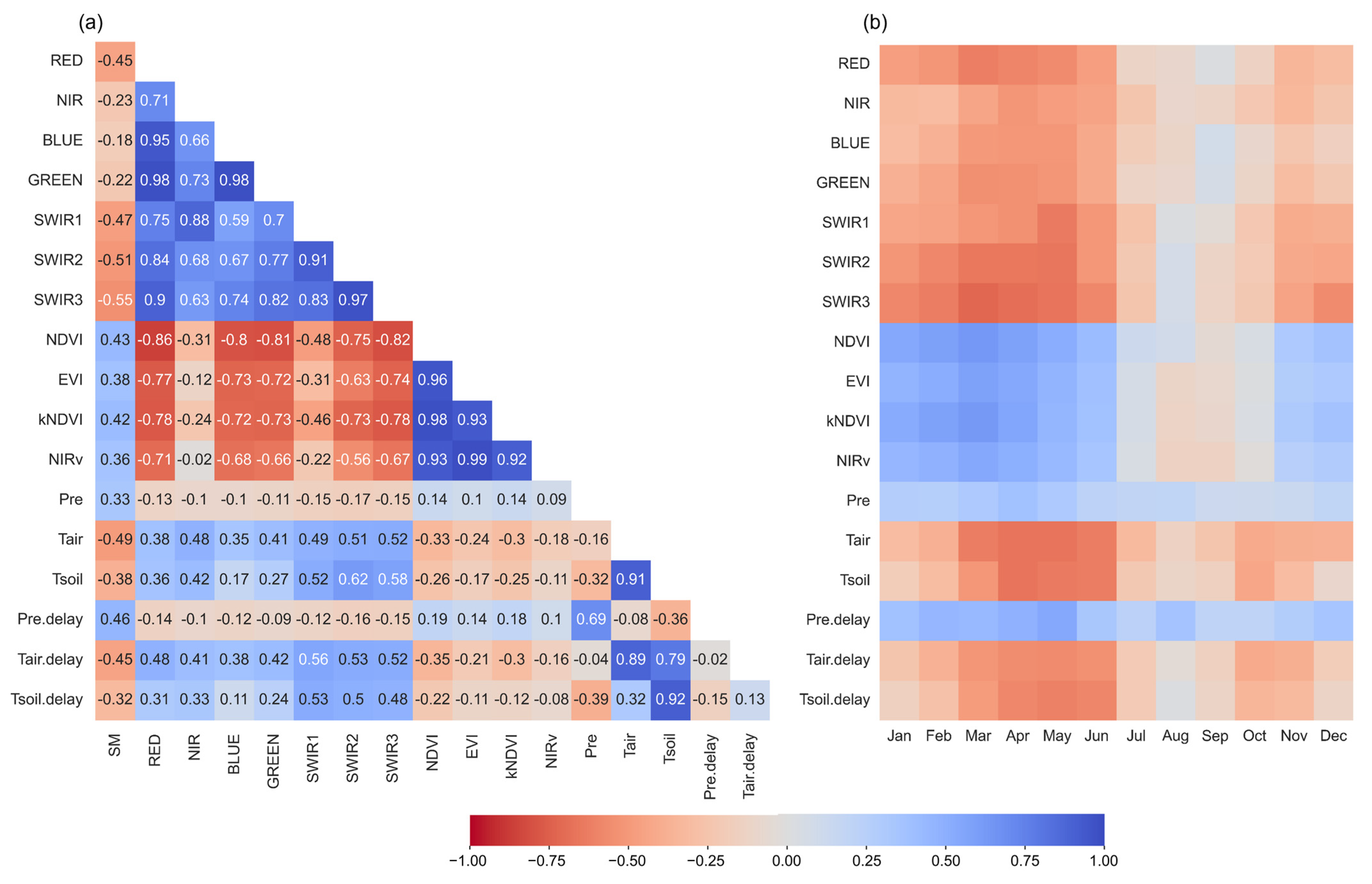
3.1. Feature Selection

Figure 4a displays the overall correlation between the input variables. In this study, the R values between the input variables and SM greater than 0.25 in absolute value are considered appropriate feature variables for SM downscaling. We observe a positive correlation between all vegetation indices and SM. Conversely, the surface reflectance across seven spectral bands is negatively correlated with SM, and there is also a negative correlation between temperature, soil temperature, and SM. Precipitation is slightly positively correlated with SM, and notably, the correlation between SM and precipitation data delayed by one day is stronger than that of contemporaneous precipitation.

It is important to emphasize that our primary focus lies in the generalization capability and accuracy of the SMNet downscaling model. Since DL is highly dependent on massive data and uses non-linear activation functions, the collinearities among variables usually does not affect the predictive ability of the model. Meanwhile, DL is robust to a certain extent, and its powerful non-linear fitting ability can automatically learn the correlation and weight redistribution between input features, so the collinearities among variables have less impact on DL. And the inclusion of additional covariates results in an augmented number of samples contributing to the downscaling model, potentially improving the overall accuracy. Therefore, input variables with high correlations have not been excluded.

We also examine the temporal variations of R between the input variables and SM (Figure 4b). The results indicate that the correlations between the input variables and SM vary over time, particularly during the months of July–October in which the correlation changes from negative to positive for the surface reflectance variable, or from positive to negative for vegetation indices. Furthermore, the correlations between some variables (e.g., air temperature and precipitation) and SM tend to be weakened. In the feature-selection phase, we retain features with a correlation exceeding 0.25 with ESA CCI SM. In addition, soil temperature was used to train the model, but it did not improve the accuracy of SMNet predictions. Therefore, soil temperature is ultimately not used in this study. Overall, 15 features, including NDVI, EVI, kNDVI, NIRv, RED, SWIR1, SWIR2, SWIR3, Tair, Pre, Tair.delay, Pre.delay, and time-invariant data (land cover, DEM, and land mask), are selected to train the SMNet model.

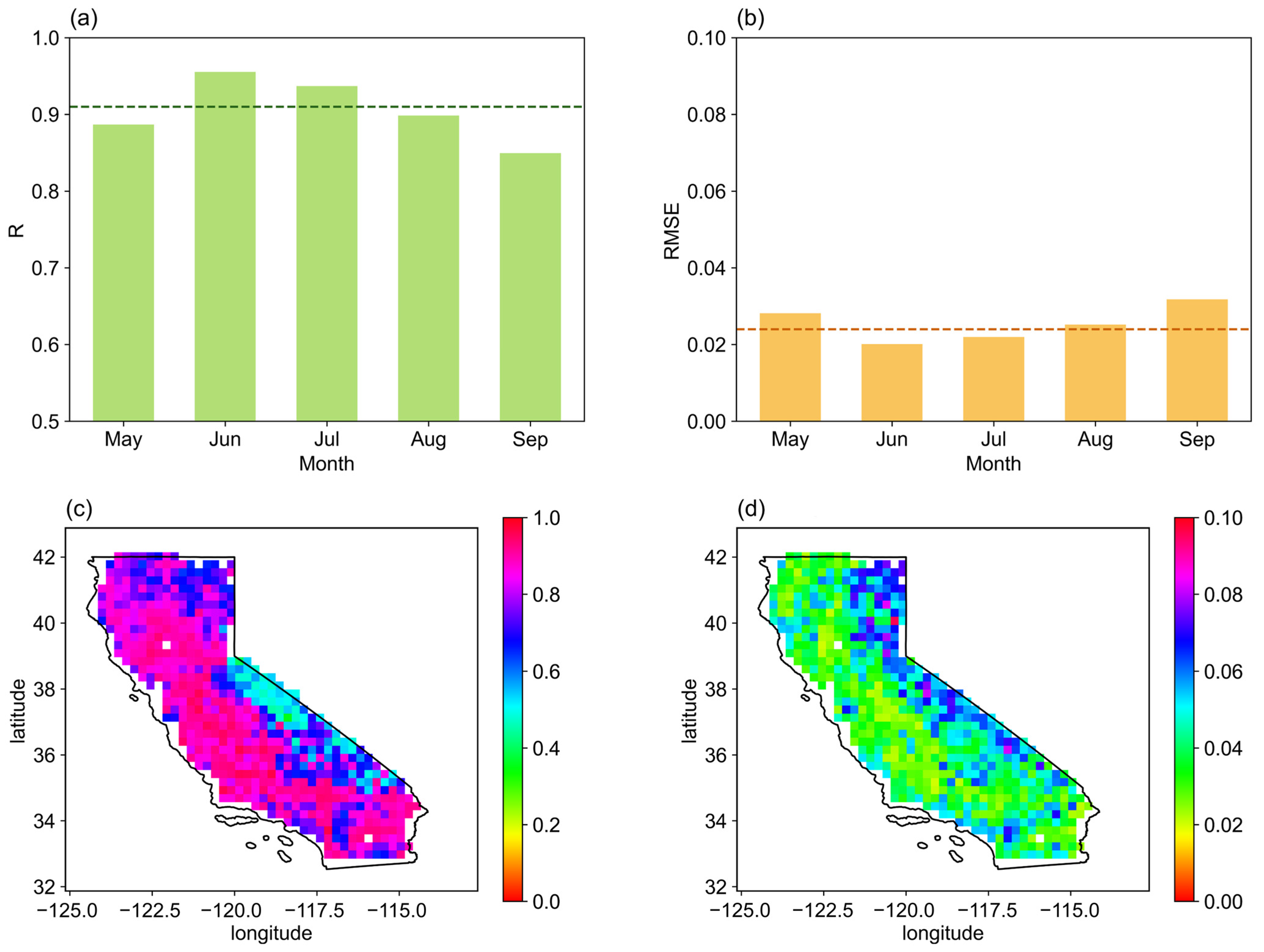
3.2. SMNet Model Performance Compared with the Original ESA CCI SM Data

Before applying the SMNet model to downscale SM at 1 km, the performance should be evaluated with the original ESA CCI SM data at a spatial resolution of 25 km. From Figure 5, we can observe an overall R of 0.91 and an overall RMSE of 0.024 m³/m³ between the estimated SM from the SMNet model and the ESA CCI SM data, indicating that the optimal SMNet model shows no signs of overfitting and demonstrates effective generalization to data beyond the training dataset. It is crucial to emphasize that the model’s performance fluctuates over time. The model achieves its highest accuracy in June and the lowest in September, as indicated by the R value of 0.96 and the RMSE value of 0.02 m³/m³ in June, and 0.85 and 0.031 m³/m³ in September. This may be closely related to vegetation growth in California. In the Californian region, June is a season of rapid vegetation growth, with an increased demand for SM by plants, leading to more pronounced changes in SM. In contrast, in September, vegetation growth may slow down, resulting in a relatively lower demand for SM. The model’s sensitivity to vegetation may contribute to differences in prediction accuracy across different months.

Figure 5c,d illustrate the spatial distributions of R and RMSE. The spatial mean R value is generally around 0.5 in the eastern part of California, particularly around the Sierra Nevada mountains. In the western and southwestern regions of California, the correlation can reach up to 0.8. The northern forested areas and southern desert regions exhibit correlations between 0.6 and 0.8. The spatial pattern of RMSE closely resembles that of R. In summary, the SMNet downscaling model is able to and has a good ability to learn the relationships between the features and the target ESA CCI SM well at a coarse resolution.

We further evaluate the downscaled 1 km SM data with the original ESA CCI SM data by resampling the downscaled SM data to 25 km. Figure 6 demonstrates a strong agreement between the downscaled SM data and the ESA CCI SM data. This is supported by the R values ranging from 0.79 (May) to 0.84 (July), with a mean value of 0.82, and an RMSE between 0.045 m³/m³ and 0.061 m³/m³, with a mean value of 0.052 m³/m³. The accuracy of the downscaling model has slightly decreased at the 1 km resolution, which may be attributed to the inherent uncertainty from the resampled input variables during the training procedure. But overall, the model’s performance is robust, and its predictive accuracy remains acceptable. This result is also supported by the spatial patterns of R and RMSE, which show that the SMNet model has good performance in the northern California coastal region and the western coastal and central regions, but a high uncertainty in the Sierra Nevada region of eastern California. The high uncertainty in eastern California is mainly caused by many pronounced missing values of SM in the mountainous areas, exacerbated by the variable topography of the mountains.

3.3. Evaluation of the Downscaled SM Data with In Situ Measurements

The downscaled SM data at 1 km resolution are additionally validated using in situ SM data collected from the ISMN network from 1 May to 30 September 2019–2021. Figure 7 displays the spatial distributions of the R and RMSE values for all in situ SM sites. The results reveal that over 64% of the sites observe R values higher than 0.60, and more than 53% obtain RMSE values below 0.08 m³/m³. Meanwhile, high R values are mainly found in most regions of California, except for a few sites near the Sierra Nevada region.

We compare the performance of the original ESA CCI SM data and the downscaled SM estimates at three SM observation networks, and the evaluation results are listed in

Table 4. Evaluation metrics of ESA CCI and downscaled SM data against in situ measurements at network scale.

In Situ	ESA CCI SM		Downscaled SM
	R	RMSE m3/m3	R	RMSE m3/m3
SCAN	0.56	0.093	0.62	0.077
SNOTEL	0.60	0.104	0.63	0.093
USCRN	0.71	0.070	0.75	0.078

. The original ESA CCI SM data have the highest accuracy in the USCRN with a high R value of 0.71 and a low RMSE of 0.070 m³/m³, compared to its performance in the SNOTEL (R = 0.60 and RMSE = 0.104 m³/m³) and the SCAN (R = 0.56 and RMSE = 0.093 m³/m³). Similarly, the downscaled SM data from the SMNet model have better performance in the USCRN than in the SCAN and the SNOTEL according to the R and RMSE values. We present the detailed results for each site in

Table A1. Evaluation metrics of ESA CCI and downscaled SM data against in situ measurements in SCAN.

SCAN	ESA CCI SM		Downscaled SM
	R	RMSE m3/m3	R	RMSE m3/m3
Ash Valley	0.79	0.138	0.83	0.085
Bodie Hills	0.73	0.076	0.73	0.064
Cochora Ranch	0.89	0.083	0.90	0.044
Death Valley Jct	0.72	0.085	0.75	0.062
Deep Springs	0.62	0.054	0.70	0.047
Doe Ridge	0.29	0.080	0.36	0.050
Eagle Lake	0.12	0.124	0.26	0.079
Essex	0.09	0.087	0.23	0.073
Ford Dry Lake	0.55	0.093	0.57	0.085
French Gulch	0.23	0.117	0.35	0.107
Marble Creek	0.57	0.100	0.67	0.110
Monocline Ridge	0.82	0.064	0.86	0.082
Shadow Mtns	0.68	0.080	0.65	0.124
Stubblefield	0.77	0.118	0.82	0.162

,

Table A2. Evaluation metrics of ESA CCI and downscaled SM data against in situ measurements in SNOTEL network.

SNOTEL	ESA CCI SM		Downscaled SM
	R	RMSE m3/m3	R	RMSE m3/m3
Blue Lakes	0.57	0.096	0.44	0.068
Burnside Lake	0.74	0.096	0.82	0.077
Carson Pass	0.68	0.179	0.72	0.153
Css Lab	0.80	0.093	0.88	0.083
Ebbetts Pass	0.46	0.070	0.56	0.083
Echo Peak	0.66	0.073	0.67	0.077
Fallen Leaf	0.47	0.126	0.44	0.129
Forestdale Creek	0.79	0.144	0.78	0.129
Hagans Meadow	0.54	0.048	0.58	0.068
Heavenly Valley	0.39	0.327	0.34	0.252
Horse Meadow	0.73	0.088	0.70	0.073
Independence Camp	0.78	0.123	0.80	0.083
Independence Creek	0.86	0.086	0.87	0.063
Independence Lake	0.45	0.100	0.53	0.068
Leavitt Lake	0.52	0.100	0.63	0.100
Leavitt Meadows	0.68	0.054	0.71	0.067
Lobdell Lake	0.76	0.069	0.78	0.069
Monitor Pass	0.55	0.061	0.48	0.102
Poison Flat	0.52	0.205	0.55	0.157
Rubicon #2	0.51	0.077	0.64	0.067
Sonora Pass	0.64	0.051	0.62	0.082
Spratt Creek	0.43	0.119	0.44	0.105
State Line	0.53	0.066	0.62	0.053
Summit Meadow	0.53	0.081	0.65	0.074
Tahoe City Cross	0.46	0.092	0.53	0.073
Truckee #2	0.73	0.096	0.69	0.078
VirginiaLakes Ridge	0.49	0.079	0.64	0.057
Ward Creek #3	0.45	0.112	0.48	0.109

and

Table A3. Evaluation metrics of ESA CCI and downscaled SM data against in situ measurements in USCRN.

USCRN	ESA CCI SM		Downscaled SM
	R	RMSE m3/m3	R	RMSE m3/m3
1	0.63	0.036	0.66	0.036
2	0.84	0.118	0.87	0.107
3	0.78	0.084	0.79	0.074
4	0.84	0.085	0.89	0.091
5	0.44	0.022	0.55	0.081

. Significantly, the validation results of the SMNet model surpass those of the original ESA CCI SM data in all three networks, which means that the downscaling model based on a DL method has a satisfactory ability to obtain a correlation between the ESA CCI SM data and the input variables, and it would not cause any degradation in the accuracy of the original data.

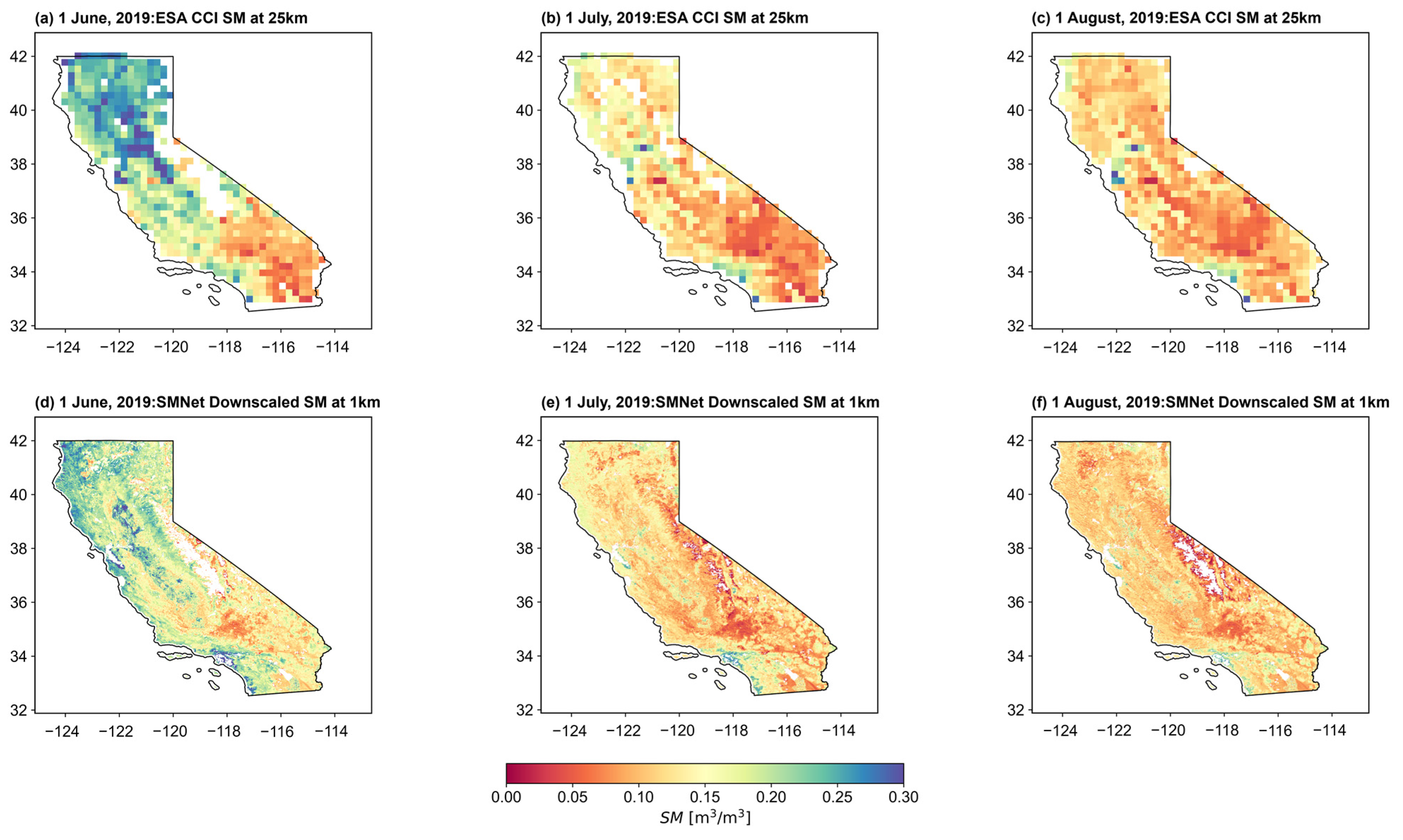
3.4. Spatial and Temporal Variation of the Downscaled ESA CCI SM Data

In this section, we investigate the spatial consistency between the original ESA CCI SM data and the downscaled SM data. The SM maps of the ESA CCI SM data and the downscaled SM data at 1 km resolution on 1 June 1, 1 July, and 1 August 2019 are selected for comparison. Compared to the coarse SM data (Figure 8a–c), the downscaled SM data (Figure 8d–f) show similar spatial patterns but more detailed variations. Examining the SM spatial distribution in Figure 8a,d, we observe relatively high SM values in the western and northern regions, but low SM values in the southeastern and southwestern regions. It is noteworthy that the downscaled SM maps present a more detailed pattern of variations, indicating a more accurate spatial variability of downscaled SM data compared to the original SM data with 25 km resolution. In July and August (Figure 8), SM values tend to be decreased across the study area, and the downscaled SM values demonstrate similar spatial patterns. These findings suggest that the downscaled SM data effectively reflect the characteristics of the original SM data. Overall, in the southeastern part of California, particularly in the Colorado Desert, perennial aridity and water scarcity are prevalent issues. The downscaled SM maps accurately highlight the textural qualities of SM across this region, providing robust support for our in-depth understanding of SM conditions in complex terrains.

In addition, the original ESA CCI SM maps are incomplete in their spatial coverage of the study area. While the downscaled SM maps provide relatively comprehensive coverage in the study area, they still contain some missing values. This may be due to the complex terrain near mountainous areas and snow accumulation at high altitudes. In summary, the downscaled SM maps are spatially coherent with those of the original ESA CCI SM data, and they capture more detailed spatial variation.

Considering the good performance of the SMNet model in terms of spatial coverage, we further validate the performance of the SMNet model in the temporal extrapolation. Here, we run the SMNet model during the non-growing season and compare the monthly average ESA CCI SM and downscaled SM data over the time period from January 2019 until December 2021. We aggregate the daily SM data at the monthly scale, and Figure 9 presents the monthly time series. As time changes, SM values display a pronounced seasonal dynamic, characterized by high SM values during the winter months and low SM values during the summer months. In comparison to the original ESA CCI SM data, the downscaled SM values exhibit systematic underestimation, especially during the winter season. The gap between the original ESA CCI SM and downscaled SM data is small during the growing season (i.e., June, July, and August), and SM reaches extremely low values in summer. Generally, the downscaled SM data illustrate a consistent seasonal variation with the original SM data, although there is relatively obvious underestimation in winter.

4. Discussion

4.1. Impact of the Input Datasets on Downscaling Efforts

In this study, we solely rely on a CNN and attentional mechanisms to explore the links between environmental factors and ESA CCI SM and to build our downscaling model (i.e., the SMNet model). The downscaling model is trained by using the high-spatial resolution input datasets. Therefore, the performance of the downscaling model is largely contingent on the precision of the input datasets.

Changes in the surface characteristics (e.g., surface reflectance) and atmospheric conditions influence the spatial and temporal variability of SM [62]. This is reasonable because SM retrieval represents the signals from the upper layer of the soil, strongly affected by the land atmosphere interactions [63]. In addition, the study period mainly focuses on the growing season (i.e., the warm and dry season), when abundant radiation and rapid vegetation growth have greater impacts on SM variability. Surface reflectance plays an important role in the SM downscaling model. Previous research has depicted a conventional exponential correlation between surface reflectance and SM [64]. In this study, we observe that precipitation has a legacy effect on SM, because it can be retained in the soil and thereby affect SM continuously over a time period, which emphasizes the important role of one-day delayed precipitation data in SM downscaling models. Surface reflectance, vegetation indices, climatic conditions, and topographic factors are the main factors affecting SM downscaling, although their influences vary across different regions or vegetation types, which is consistent with many previous studies [65,66,67].

Previous studies have revealed that soil temperature gives a better indication of the rate of heating and cooling of the soil, which maybe reflect related information about SM variation [68]. This implies that soil temperature can be used as a suitable factor for downscaling SM data. Based on the implied functional correlation between SM and soil temperature, some researchers preliminarily tested this potential relationship and found that the downscaling of SM data using soil temperature was promising [69]. We additionally add soil temperature as an input variable to drive the downscaling model, and evaluate the performance of the model by using the validation set. The values of R and RMSE are 0.82 and 0.056, respectively. Comparing the results with the SMNet model without soil temperature, adding soil temperature as an input variable for SM downscaling results in a degradation in model performance, which could be attributed to the strong correlation between soil temperature and air temperature, and the supplemental auxiliary information offered does not sufficiently offset the uncertainty that it generates.

In order to identify the impacts of the input variables on model performance, we conduct a series of ablation experiments. We utilize all variables input into the model as the baseline model and systematically eliminate each input variable. The elimination order comprises MODIS surface reflectance, vegetation index (VI), mean air temperature (Tair), precipitation (prep), digital elevation model (DEM), and land mask. According to the seven ablation experiments (

Table 5. Validation results for feature importance ablation studies.

Approach	R	RMSE m3/m3
SMNet	0.91	0.024
SMNet-surface reflectance	0.81	0.043
SMNet-VI	0.83	0.039
SMNet-Tair	0.84	0.038
SMNet-prep	0.79	0.048
SMNet-DEM	0.75	0.052
SMNet-LM	0.86	0.031

Note: SMNet: with all selected input variables, SMNet-surface reflectance: model without MODIS surface reflectance data, SMNet-VI: model without VI, SMNet-Tair: model without mean air temperature, SMNet-prep: model without precipitation, SMNet-DEM: model without DEM, and SMNet-LM: model without land mask.

), we find a significant performance decline upon excluding the DEM variable (i.e., SMNet-DEM in Table 5), suggesting its critical importance for SM downscaling in complex terrains. In addition, precipitation is the second most important driver for SM downscaling, which indicates the important role of precipitation in spatiotemporal variation of soil moisture. In contrast, surface reflectance, vegetation indices, and air temperature have relatively smaller impacts on SM downscaling.

To achieve high spatial coverage of downscaled SM maps, spatially and temporally continuous high-resolution auxiliary data are a prerequisite for the downscaled SM models. However, the optical RS data (particularly for vegetation indices) are vulnerable to cloud and rain coverage, so these auxiliary data cannot be available for all-region and all-weather conditions. Future work needs to consider microwave RS data and land surface model outputs as input data or reconstruct the optical RS data.

4.2. The Impact of Different Methods in Downscaling Models

4.2.1. Comparison with Other Published Methods for Downscaling ESA CCI SM Data

As shown in

Table 6. Application of different methods in ESA CCI SM downscaling studies.

Source	Approaches	Study Area	Spatial Resolution	RMSE of In Situ Site Validation (m3/m3)
Zhao et al. [30]	Statistical model data fusion (GWR + ATPK)	Iberian Peninsula	1 km	0.091
Song et al. [72]	Statistical model data fusion (TVDI + SVCT)	Nagqu, and Qinghai–Tibet Plateau	1 km	0.057
Liu et al. [75]	CART, KNN, BAYE, and RF	Three northeastern provinces of China	1 km	0.076 0.074 0.075 0.073
Peng et al. [73]	Statistical model (VTCI)	Yunnan Province, China,	1 km	0.078
Shangguan et al. [76]	DL (CNN + Attention)	Qinghai–Tibet Plateau	1 km	0.099
Kovačević et al. [74]	RF	California, USA	1 km	0.052 (PBO_H2O); 0.085 (SCAN); 0.090 (USCRN).
Our study	DL (CNN + Attention)	California, USA	1 km	0.077 (SCAN); 0.093 (SNOTEL); 0.078 (USCRN).

, traditional SM downscaling methods typically rely on physical hydrological models [70], statistical models [71], or data fusion approaches [30,72,73]. Machine learning methods employ algorithms such as the random forest and the support vector machine to establish complex relationships between SM and surface variables [74,75]. These methods predict SM by learning from extensive training data without relying on physical hydrological models or statistical assumptions. DL methods have the potential to automatically extract features and learn complex spatial and temporal patterns in the presence of large-scale data and intricate relationships [76].

However, the application of DL methods incorporating attention mechanisms in SM downscaling research remains underexplored. Shangguan et al. [76] attempted to use attention mechanisms to downscale ESA CCI SM data, achieving results similar to our proposed method. Nevertheless, our study introduces a more concise model capable of achieving comparable downscaling performance to that of Shangguan et al. [76].

In the investigation into downscaling ESA CCI SM data for the Californian region, we utilized a deep learning method with an attention mechanism, which has superior performance compared with the random forest method used by Kovačević et al. [74]. This suggests that the attention-based DL methods may have a relative advantage in SM downscaling tasks compared to conventional machine learning methods. Meanwhile, despite differences between the study areas that we selected and those covered in other studies, our research demonstrates comparable accuracy levels.

4.2.2. The IMPACT of the Attention Mechanism in the Downscaling Model

Recently, DL methods have been considered to have better performance than traditional shallow network architectures in revealing deeper non-linear relationships among immense datasets and numerous features [36,77]. Therefore, the use of DL methods in SM downscaling has gradually become widespread. Nevertheless, the current studies of DL methods containing attention mechanisms in SM downscaling are few. Unlike the DL frameworks used in previous SM downscaling studies, we established a DL downscaling model that incorporates an attention mechanism, which is the first attempt to downscale ESA CCI SM data based on the CBAM attention mechanism in a DL model. Here, we conducted five experiments, namely, (1) no attention module; (2) the Convolution Block Attention Module (CBAM); (3) Polarized Self-Attention (PSA); (4) the Dual-Attention Network (DAN); (5) the Squeeze-and-Excitation Network (SENet), to examine the necessity of the attention mechanism module in the downscaling of SM models.

Table 7. Results of other schemes after optimization for test set of California.

Experiments	Statistical Metrics
	R	RMSE m3/m3
(1) no attention module	0.63	0.051
(2) CBAM	0.91	0.024
(3) PSA	0.88	0.029
(4) DAN	0.86	0.032
(5) SENet	0.84	0.034

shows the experimental results. Experiment (1), no attention module, served as a baseline, and its R and RMSE values are 0.63 and 0.051 m³/m³, respectively, which are lower than those of the other experiments. The addition of the attention mechanism module allowed us to focus on areas of potential interest and improves the overall precision of the model. Moreover, we examined the performances of different attention mechanisms added into the DL model and their effectiveness in SM downscaling. The results demonstrated that the accuracy of the model with the addition of the CBAM is better than that of the other schemes, as evidenced by an R of 0.91 and an RMSE of 0.024. The CBAM combines the spatial and channel attention mechanisms, and thus, it can adequately extract auxiliary features. The channel attention module (CAM) separates the input tensor into two subsequent vectors of dimensionality, including global max pooling and global average pooling. Average pooling is primarily employed to consolidate spatial information, while max pooling retains more intricate contextual information, capturing the finer details of the object’s edges within the image. The spatial attention module (SAM) signifies the attention mask applied to the feature map, which will enhance the features of the defined study area. By refining the feature maps, we enhanced the input datasets to the subsequent convolutional layers, thereby improving the model’s performance.

Overall, including the CBAM gives the best results in SM downscaling, revealing the advantages of our proposed SMNet model. Therefore, the attention mechanism module is necessary to improve the model’s performance in soil moisture downscaling.

4.3. Temporal Extrapolation of the Model

In this study, we selected data from the growing season for model training, because the non-growing season in California is a wet period with numerous rainy days, which leads to seriously numerous missing values in the ESA CCI SM data. The commonly used DL models generally need abundant training samples. Unfortunately, it is often not possible to obtain suitable training samples due to the severe amount of data missing during the non-growing season in California. The SMNet model used in this study adopted a DL framework and employed convolutional and attention mechanisms to establish the relationships between input variables and SM, thereby downscaling SM. It is usually considered that the relationship between input variables and SM is constant in time, so the ability of the model trained by the growing season data can make predictions for the non-growing season data (similar to transfer learning). To our knowledge, no studies have investigated transfer learning for SM downscaling that distinguishes between growing season and non-growing season data. Therefore, here, we discussed the temporal extrapolation capability of the SMNet model.

For this purpose, we used data from the non-growing season to make predictions. As illustrated in Figure 10, R is predominantly above 0.6 (the mean R is 0.67), and RMSE is always below 0.07 (the mean RMSE is 0.063), which implies that the SMNet model has an acceptable performance in temporal extrapolation. It should be noted that the model’s performance is relatively lower from December to March compared to the other seasons, which may be due to changes in climatic conditions that further altered the correlation between SM and input data, or vegetation dormancy/frozen soil caused by rain and snow which caused the inputs failing to reflect these characteristics.

4.4. Uncertainty of the Downscaling Results

DL-based downscaling methods demonstrate a compelling capability to capture non-linear relationships. Additionally, the effectiveness of DL methods in predicting SM has been extensively validated in numerous studies [76,78]. In this study, the accuracy and efficiency of the SMNet model are highly dependent on those optical RS data utilized and on data preprocessing [79,80]. In the data preprocessing stage, the input variables at different spatial resolutions were resampled to a 25 km spatial resolution by using a bilinear interpolation method. However, this method has its potential limitations when resampling high-resolution RS data to relatively coarse resolution data. We compared three resampling methods, including bilinear, cubic, and first order conservative resampling (in Figure A1), and we found that although the three resampling methods all kept the spatial characteristics of the raw data, bilinear and cubic resampling methods were not able to perfectly capture the fine spatial pattern. By contrast, the first order conservative resampling method yielded the best spatial consistency with the raw high-resolution RS data. Therefore, we recommend using the first order conservative method for RS data resampling.

The validation results (Figure 8) demonstrate that the spatial arrangement of the downscaled SM data from the SMNet model is concordant with that of the original ESA CCI SM data. Moreover, the specific spatial details of the downscaled SM maps are enhanced by the SMNet model. Nevertheless, we noticed abnormally low downscaled SM values in the eastern study area. In the eastern part of the study area, which is the Sierra Nevada mountains, the region is covered by limited alpine grassland, exposed bedrock, and snow at high altitudes. This leads to a large number of missing values in both the ESA CCI SM data and MODIS data for this region, which affects the training of the SMNet model, decreases the accuracy of SM downscaling, and leads to extremely low downscaled SM values.

Derived from the in situ SM measurement data, the site validation results (Figure 7) indicate that the R values obtained from downscaled SM and in situ SM data are greater than 0.6, with some sites even exceeding 0.8. However, there are some sites with correlations below 0.5. The reason for this phenomenon may be that the correlation between the original ESA CCI SM data and the in situ SM data is inherently low, and the training data for the downscaling model is based on the original ESA CCI SM data. On the other hand, this limitation arises primarily from the utilization of conventional point-scale SM monitoring methods in the networks, and so these methods are unable to reflect downscaled SM data accurately at the 1 km resolution scale [81]. Therefore, the variabilities in SM values from point-scale measurements within the given networks are found to be larger than those from the downscaled SM values. This is obvious particularly for sites with severe spatial heterogeneity, such as differing topographies, climate conditions, soil properties, vegetation, or land cover types. Although the correlation varies from site to site, the correlation between the in situ data and the downscaled data is higher than that with the original ESACCI SM data. As can be seen in Figure 8, the correlation is lower in high mountainous and rugged terrain, partly because of the complex surface roughness of the in situ coverage. This leads to some bias in the instrument measurements [82,83].

We further assessed the temporal coherence between the original ESA CCI SM data and the downscaled SM data. Throughout the study period (2019–2021), high SM values are predominantly observed during January, February, March, and December, while low values are frequently found during July, August, and September (Figure 9). This is likely due to the high levels of evapotranspiration during the summer months, caused by high temperatures and vigorous plant growth. California’s Mediterranean climate brings an abundance of precipitation during the winter months, which is efficiently retained by lower temperatures and weak plant evapotranspiration, resulting in relatively high SM. On a monthly scale, the downscaled SM data are underestimated in winter, while the overall temporal trend of the downscaled SM data is consistent with the that of the original ESA CCI SM data. This indicates good robustness of the SMNet model.

The underestimation of SM is observed during the non-growing season (October-April), which may be related to the training method of our data. Alternatively, this could be due to the fact that the initial low-resolution ESA CCI SM images do not aid in describing probable regions with lower SM values. Conversely, the SMNet model can grasp more spatial intricacies, hence improving the accuracy of SM value prediction in these areas. Therefore, during some seasons with more missing data, the SMNet model serves the function of interpolating missing values.

5. Conclusions

Traditional coarse resolution SM data collected via satellites, although providing broad spatial coverage, fail to adequately meet local requirements for regional-scale hydrological analysis, crop irrigation monitoring, and land surface evapotranspiration estimation. Recently, DL downscaling algorithms have been widely applied in hydrology-related fields of RS data. In this study, we developed a DL model with the integration of a dual-attention mechanism (i.e., the SMNet model) for SM downscaling. The evaluation results demonstrate the effectiveness and feasibility of the SMNet model in SM downscaling in California with a complex terrain. The integration of attention mechanisms in the DL model enhances the performance of SM downscaling in terms of spatial coverage and temporal extrapolation.

In comparison with the original ESA CCI SM data, the downscaled SM data exhibit a mean R of 0.82 and a mean RMSE of 0.052 m³/m³. The R and RMSE (m³/m³), values in three in situ observation networks (i.e., SCAN, SNOTEL, and USCRN) are 0.62, 0.63, and 0.77, and 0.077 m³/m³, 0.093 m³/m³, and 0.078 m³/m³, respectively. Meanwhile, the validation results during the non-growing season indicate that R consistently exceeds 0.6 and RMSE remains below 0.07 m³/m³, confirming the good performance of the SMNet model in terms of spatial coverage and temporal extrapolation.

Overall, our research introduces a relatively simple but effective approach for SM downscaling with seamless spatiotemporal coverage. However, some limitations of the SMNet model exist. The SMNet model’s performance is still affected by the accuracy of input data and hyperparameter tuning, and the stability of the prediction results requires further enhancement. Future studies are required to optimize model structures, integrating additional types of high-precision auxiliary data and environmental factors and enhancing the interpretability and robustness of the model. This study contributes to the valuable exploration of DL techniques in SM downscaling and related domains, laying a foundation for future research and applications in this area.

References

1. Sun, H.; Cai, C.; Liu, H.; Yang, B. Microwave and Meteorological Fusion: A Method of Spatial Downscaling of Remotely Sensed Soil Moisture. IEEE J. Sel. Top. Appl. Earth Obs. Remote Sens. 2019, 12, 1107–1119. [Google Scholar] [CrossRef]
2. Idso, S.B.; Jackson, R.D.; Reginato, R.J.; Kimball, B.A.; Nakayama, F.S. The Dependence of Bare Soil Albedo on Soil Water Content. J. Appl. Meteorol. Climatol. 1975, 14, 109–113. [Google Scholar] [CrossRef]
3. Merlin, O.; Walker, J.P.; Chehbouni, A.; Kerr, Y. Towards Deterministic Downscaling of SMOS Soil Moisture Using MODIS Derived Soil Evaporative Efficiency. Remote Sens. Environ. 2008, 112, 3935–3946. [Google Scholar] [CrossRef]
4. Sánchez, N.; González-Zamora, Á.; Piles, M.; Martínez-Fernández, J. A New Soil Moisture Agricultural Drought Index (SMADI) Integrating MODIS and SMOS Products: A Case of Study over the Iberian Peninsula. Remote Sens. 2016, 8, 287. [Google Scholar] [CrossRef]
5. Feng, S.; Huang, X.; Zhao, S.; Qin, Z.; Fan, J.; Zhao, S. Evaluation of Several Satellite-Based Soil Moisture Products in the Continental US. Sensors 2022, 22, 9977. [Google Scholar] [CrossRef] [PubMed]
6. Kim, S.; Zhang, R.; Pham, H.; Sharma, A. A Review of Satellite-Derived Soil Moisture and Its Usage for Flood Estimation. Remote Sens. Earth Syst. Sci. 2019, 2, 225–246. [Google Scholar] [CrossRef]
7. Borodychev, V.V.; Lytov, M.N. Irrigation Management Model Based on Soil Moisture Distribution Profile. IOP Conf. Ser. Earth Environ. Sci. 2020, 577, 012022. [Google Scholar] [CrossRef]
8. Doraiswamy, P.C.; Hatfield, J.L.; Jackson, T.J.; Akhmedov, B.; Prueger, J.; Stern, A. Crop Condition and Yield Simulations Using Landsat and MODIS. Remote Sens. Environ. 2004, 92, 548–559. [Google Scholar] [CrossRef]
9. Koster, R.D.; Mahanama, S.P.P.; Yamada, T.J.; Balsamo, G.; Berg, A.A.; Boisserie, M.; Dirmeyer, P.A.; Doblas-Reyes, F.J.; Drewitt, G.; Gordon, C.T.; et al. Contribution of Land Surface Initialization to Subseasonal Forecast Skill: First Results from a Multi-Model Experiment. Geophys. Res. Lett. 2010, 37, L02402. [Google Scholar] [CrossRef]
10. Gruber, A.; Dorigo, W.A.; Zwieback, S.; Xaver, A.; Wagner, W. Characterizing Coarse-Scale Representativeness of in Situ Soil Moisture Measurements from the International Soil Moisture Network. Vadose Zone J. 2013, 12, 1–16. [Google Scholar] [CrossRef]
11. Ochsner, T.E.; Cosh, M.H.; Cuenca, R.H.; Dorigo, W.A.; Draper, C.S.; Hagimoto, Y.; Kerr, Y.H.; Larson, K.M.; Njoku, E.G.; Small, E.E.; et al. State of the Art in Large-Scale Soil Moisture Monitoring. Soil. Sci. Soc. Am. J. 2013, 77, 1888–1919. [Google Scholar] [CrossRef]
12. Tavakol, A.; McDonough, K.R.; Rahmani, V.; Hutchinson, S.L.; Hutchinson, J.M.S. The Soil Moisture Data Bank: The Ground-Based, Model-Based, and Satellite-Based Soil Moisture Data. Remote Sens. Appl. Soc. Environ. 2021, 24, 100649. [Google Scholar] [CrossRef]
13. Yuan, Q.; Shen, H.; Li, T.; Li, Z.; Li, S.; Jiang, Y.; Xu, H.; Tan, W.; Yang, Q.; Wang, J.; et al. Deep Learning in Environmental Remote Sensing: Achievements and Challenges. Remote Sens. Environ. 2020, 241, 111716. [Google Scholar] [CrossRef]
14. Babaeian, E.; Sadeghi, M.; Jones, S.B.; Montzka, C.; Vereecken, H.; Tuller, M. Ground, Proximal, and Satellite Remote Sensing of Soil Moisture. Rev. Geophys. 2019, 57, 530–616. [Google Scholar] [CrossRef]
15. Bartalis, Z.; Wagner, W.; Naeimi, V.; Hasenauer, S.; Scipal, K.; Bonekamp, H.; Figa, J.; Anderson, C. Initial Soil Moisture Retrievals from the METOP-A Advanced Scatterometer (ASCAT). Geophys. Res. Lett. 2007, 34, L20401. [Google Scholar] [CrossRef]
16. Yao, P.; Lu, H.; Shi, J.; Zhao, T.; Yang, K.; Cosh, M.H.; Gianotti, D.J.S.; Entekhabi, D. A Long Term Global Daily Soil Moisture Dataset Derived from AMSR-E and AMSR2 (2002–2019). Sci. Data 2021, 8, 143. [Google Scholar] [CrossRef]
17. Gruber, A.; Scanlon, T.; van der Schalie, R.; Wagner, W.; Dorigo, W. Evolution of the ESA CCI Soil Moisture Climate Data Records and Their Underlying Merging Methodology. Earth Syst. Sci. Data 2019, 11, 717–739. [Google Scholar] [CrossRef]
18. Kerr, Y.H.; Waldteufel, P.; Wigneron, J.-P.; Delwart, S.; Cabot, F.; Boutin, J.; Escorihuela, M.-J.; Font, J.; Reul, N.; Gruhier, C. The SMOS Mission: New Tool for Monitoring Key Elements Ofthe Global Water Cycle. Proc. IEEE 2010, 98, 666–687. [Google Scholar] [CrossRef]
19. Entekhabi, D.; Njoku, E.G.; O’neill, P.E.; Kellogg, K.H.; Crow, W.T.; Edelstein, W.N.; Entin, J.K.; Goodman, S.D.; Jackson, T.J.; Johnson, J. The Soil Moisture Active Passive (SMAP) Mission. Proc. IEEE 2010, 98, 704–716. [Google Scholar] [CrossRef]
20. Kerr, Y.H.; Waldteufel, P.; Wigneron, J.-P.; Martinuzzi, J.; Font, J.; Berger, M. Soil Moisture Retrieval from Space: The Soil Moisture and Ocean Salinity (SMOS) Mission. IEEE Trans. Geosci. Remote Sens. 2001, 39, 1729–1735. [Google Scholar] [CrossRef]
21. Das, N.N.; Entekhabi, D.; Dunbar, R.S.; Colliander, A.; Chen, F.; Crow, W.; Jackson, T.J.; Berg, A.; Bosch, D.D.; Caldwell, T.; et al. The SMAP Mission Combined Active-Passive Soil Moisture Product at 9 km and 3 km Spatial Resolutions. Remote Sens. Environ. 2018, 211, 204–217. [Google Scholar] [CrossRef]
22. Piles, M.; Petropoulos, G.P.; Sánchez, N.; González-Zamora, Á.; Ireland, G. Towards Improved Spatio-Temporal Resolution Soil Moisture Retrievals from the Synergy of SMOS and MSG SEVIRI Spaceborne Observations. Remote Sens. Environ. 2016, 180, 403–417. [Google Scholar] [CrossRef]
23. Sun, H.; Zhou, B.; Zhang, C.; Liu, H.; Yang, B. DSCALE_mod16: A Model for Disaggregating Microwave Satellite Soil Moisture with Land Surface Evapotranspiration Products and Gridded Meteorological Data. Remote Sens. 2020, 12, 980. [Google Scholar] [CrossRef]
24. Leroux, D.J.; Das, N.N.; Entekhabi, D.; Colliander, A.; Njoku, E.; Jackson, T.J.; Yueh, S. Active–Passive Soil Moisture Retrievals during the SMAP Validation Experiment 2012. IEEE Geosci. Remote Sens. Lett. 2016, 13, 475–479. [Google Scholar] [CrossRef]
25. Wu, X.; Walker, J.P.; Rüdiger, C.; Panciera, R.; Gao, Y. Intercomparison of Alternate Soil Moisture Downscaling Algorithms Using Active–Passive Microwave Observations. IEEE Geosci. Remote Sens. Lett. 2016, 14, 179–183. [Google Scholar] [CrossRef]
26. Shangguan, Y.; Min, X.; Shi, Z. Inter-Comparison and Integration of Different Soil Moisture Downscaling Methods over the Qinghai-Tibet Plateau. J. Hydrol. 2023, 617, 129014. [Google Scholar] [CrossRef]
27. Peng, J.; Loew, A.; Merlin, O.; Verhoest, N.E.C. A Review of Spatial Downscaling of Satellite Remotely Sensed Soil Moisture. Rev. Geophys. 2017, 55, 341–366. [Google Scholar] [CrossRef]
28. Sabaghy, S.; Walker, J.P.; Renzullo, L.J.; Jackson, T.J. Spatially Enhanced Passive Microwave Derived Soil Moisture: Capabilities and Opportunities. Remote Sens. Environ. 2018, 209, 551–580. [Google Scholar] [CrossRef]
29. Zhu, Z.; Bo, Y.; Sun, T. Spatial Downscaling of Satellite Soil Moisture Products Based on Apparent Thermal Inertia: Considering the Effect of Vegetation Condition. J. Hydrol. 2023, 616, 128824. [Google Scholar] [CrossRef]
30. Zhao, W.; Wen, F.; Wang, Q.; Sanchez, N.; Piles, M. Seamless Downscaling of the ESA CCI Soil Moisture Data at the Daily Scale with MODIS Land Products. J. Hydrol. 2021, 603, 126930. [Google Scholar] [CrossRef]
31. Song, P.; Huang, J.; Mansaray, L.R. An Improved Surface Soil Moisture Downscaling Approach over Cloudy Areas Based on Geographically Weighted Regression. Agric. For. Meteorol. 2019, 275, 146–158. [Google Scholar] [CrossRef]
32. Kolassa, J.; Reichle, R.H.; Draper, C.S. Merging Active and Passive Microwave Observations in Soil Moisture Data Assimilation. Remote Sens. Environ. 2017, 191, 117–130. [Google Scholar] [CrossRef]
33. Hu, F.; Wei, Z.; Zhang, W.; Dorjee, D.; Meng, L. A Spatial Downscaling Method for SMAP Soil Moisture through Visible and Shortwave-Infrared Remote Sensing Data. J. Hydrol. 2020, 590, 125360. [Google Scholar] [CrossRef]
34. Wei, Z.; Meng, Y.; Zhang, W.; Peng, J.; Meng, L. Downscaling SMAP Soil Moisture Estimation with Gradient Boosting Decision Tree Regression over the Tibetan Plateau. Remote Sens. Environ. 2019, 225, 30–44. [Google Scholar] [CrossRef]
35. Liu, Y.; Jing, W.; Wang, Q.; Xia, X. Generating High-Resolution Daily Soil Moisture by Using Spatial Downscaling Techniques: A Comparison of Six Machine Learning Algorithms. Adv. Water Resour. 2020, 141, 103601. [Google Scholar] [CrossRef]
36. Zhao, H.; Li, J.; Yuan, Q.; Lin, L.; Yue, L.; Xu, H. Downscaling of Soil Moisture Products Using Deep Learning: Comparison and Analysis on Tibetan Plateau. J. Hydrol. 2022, 607, 127570. [Google Scholar] [CrossRef]
37. Jiang, M.; Shen, H.; Li, J. Cycle GAN Based Heterogeneous Spatial-Spectral Fusion for Soil Moisture Downscaling. In Proceedings of the IGARSS 2022—2022 IEEE International Geoscience and Remote Sensing Symposium, Kuala Lumpur, Malaysia, 17–22 July 2022; pp. 4819–4822. [Google Scholar]
38. Sit, M.; Demiray, B.Z.; Demir, I. Spatial Downscaling of Streamflow Data with Attention Based Spatio-Temporal Graph Convolutional Networks [Preprint], EarthArXiv. Available online: https://eartharxiv.org/repository/view/5227/ (accessed on 4 September 2023). [CrossRef]
39. Liu, G.; Zhang, R.; Hang, R.; Ge, L.; Shi, C.; Liu, Q. Statistical Downscaling of Temperature Distributions in Southwest China by Using Terrain-Guided Attention Network. IEEE J. Sel. Top. Appl. Earth Obs. Remote Sens. 2023, 16, 1678–1690. [Google Scholar] [CrossRef]
40. Zhang, L.; Liu, Y.; Ren, L.; Teuling, A.J.; Zhang, X.; Jiang, S.; Yang, X.; Wei, L.; Zhong, F.; Zheng, L. Reconstruction of ESA CCI Satellite-Derived Soil Moisture Using an Artificial Neural Network Technology. Sci. Total Environ. 2021, 782, 146602. [Google Scholar] [CrossRef]
41. Dorigo, W.; Wagner, W.; Albergel, C.; Albrecht, F.; Balsamo, G.; Brocca, L.; Chung, D.; Ertl, M.; Forkel, M.; Gruber, A.; et al. ESA CCI Soil Moisture for Improved Earth System Understanding: State-of-the Art and Future Directions. Remote Sens. Environ. 2017, 203, 185–215. [Google Scholar] [CrossRef]
42. Gensheimer, J.; Turner, A.J.; Köhler, P.; Frankenberg, C.; Chen, J. A Convolutional Neural Network for Spatial Downscaling of Satellite-Based Solar-Induced Chlorophyll Fluorescence (SIFnet). Biogeosciences 2022, 19, 1777–1793. [Google Scholar] [CrossRef]
43. Huete, A.; Didan, K.; Miura, T.; Rodriguez, E.P.; Gao, X.; Ferreira, L.G. Overview of the Radiometric and Biophysical Performance of the MODIS Vegetation Indices. Remote Sens. Environ. 2002, 83, 195–213. [Google Scholar] [CrossRef]
44. Du, J.; Kimball, J.; Chan, S.; Colliander, A.; Carroll, M. Evaluation of Surface Fractional Water Impacts on SMAP Soil Moisture Retrieval. AGU Fall Meet. Abstr. 2021, 2021, H15W–1312. [Google Scholar]
45. Koster, R.D.; Suarez, M.J.; Higgins, R.W.; Van den Dool, H.M. Observational Evidence That Soil Moisture Variations Affect Precipitation. Geophys. Res. Lett. 2003, 30, 1241. [Google Scholar] [CrossRef]
46. Funk, C.; Peterson, P.; Landsfeld, M.; Pedreros, D.; Verdin, J.; Shukla, S.; Husak, G.; Rowland, J.; Harrison, L.; Hoell, A.; et al. The Climate Hazards Infrared Precipitation with Stations—A New Environmental Record for Monitoring Extremes. Sci. Data 2015, 2, 150066. [Google Scholar] [CrossRef] [PubMed]
47. Arregocés, H.A.; Rojano, R.; Pérez, J. Validation of the CHIRPS Dataset in a Coastal Region with Extensive Plains and Complex Topography. Case Stud. Chem. Environ. Eng. 2023, 8, 100452. [Google Scholar] [CrossRef]
48. Bai, L.; Shi, C.; Li, L.; Yang, Y.; Wu, J. Accuracy of CHIRPS Satellite-Rainfall Products over Mainland China. Remote Sens. 2018, 10, 362. [Google Scholar] [CrossRef]
49. Nawaz, M.; Iqbal, M.F.; Mahmood, I. Validation of CHIRPS Satellite-Based Precipitation Dataset over Pakistan. Atmos. Res. 2021, 248, 105289. [Google Scholar] [CrossRef]
50. Ocampo-Marulanda, C.; Fernández-Álvarez, C.; Cerón, W.L.; Canchala, T.; Carvajal-Escobar, Y.; Alfonso-Morales, W. A Spatiotemporal Assessment of the High-Resolution CHIRPS Rainfall Dataset in Southwestern Colombia Using Combined Principal Component Analysis. Ain Shams Eng. J. 2022, 13, 101739. [Google Scholar] [CrossRef]
51. Crow, W.T.; Berg, A.A.; Cosh, M.H.; Loew, A.; Mohanty, B.P.; Panciera, R.; de Rosnay, P.; Ryu, D.; Walker, J.P. Upscaling Sparse Ground-Based Soil Moisture Observations for the Validation of Coarse-Resolution Satellite Soil Moisture Products. Rev. Geophys. 2012, 50, RG2002. [Google Scholar] [CrossRef]
52. Coleman, M.L.; Niemann, J.D. Controls on Topographic Dependence and Temporal Instability in Catchment-Scale Soil Moisture Patterns. Water Resour. Res. 2013, 49, 1625–1642. [Google Scholar] [CrossRef]
53. Ranney, K.J.; Niemann, J.D.; Lehman, B.M.; Green, T.R.; Jones, A.S. A Method to Downscale Soil Moisture to Fine Resolutions Using Topographic, Vegetation, and Soil Data. Adv. Water Resour. 2015, 76, 81–96. [Google Scholar] [CrossRef]
54. Farr, T.G.; Rosen, P.A.; Caro, E.; Crippen, R.; Duren, R.; Hensley, S.; Kobrick, M.; Paller, M.; Rodriguez, E.; Roth, L.; et al. The Shuttle Radar Topography Mission. Rev. Geophys. 2007, 45, RG2004. [Google Scholar] [CrossRef]
55. Van Doninck, J.; Peters, J.; De Baets, B.; De Clercq, E.M.; Ducheyne, E.; Verhoest, N.E.C. The Potential of Multitemporal Aqua and Terra MODIS Apparent Thermal Inertia as a Soil Moisture Indicator. Int. J. Appl. Earth Obs. Geoinf. 2011, 13, 934–941. [Google Scholar] [CrossRef]
56. Woo, S.; Park, J.; Lee, J.-Y.; Kweon, I.S. CBAM: Convolutional Block Attention Module. In Proceedings of the European Conference on Computer Vision (ECCV), Munich, Germany, 8–14 September 2018; pp. 3–19. [Google Scholar]
57. Liu, J.; Zhang, Y.; Liu, C.; Liu, X. Monitoring Impervious Surface Area Dynamics in Urban Areas Using Sentinel-2 Data and Improved Deeplabv3+ Model: A Case Study of Jinan City, China. Remote Sens. 2023, 15, 1976. [Google Scholar] [CrossRef]
58. Ma, R.; Wang, J.; Zhao, W.; Guo, H.; Dai, D.; Yun, Y.; Li, L.; Hao, F.; Bai, J.; Ma, D. Identification of Maize Seed Varieties Using MobileNetV2 with Improved Attention Mechanism CBAM. Agriculture 2023, 13, 11. [Google Scholar] [CrossRef]
59. Brunet, D.; Vrscay, E.R.; Wang, Z. On the Mathematical Properties of the Structural Similarity Index. IEEE Trans. Image Process. 2012, 21, 1488–1499. [Google Scholar] [CrossRef] [PubMed]
60. Wang, Z.; Bovik, A.C. Mean Squared Error: Love It or Leave It? A New Look at Signal Fidelity Measures. IEEE Signal Process. Mag. 2009, 26, 98–117. [Google Scholar] [CrossRef]
61. Kang, S.-J. SSIM Preservation-Based Backlight Dimming. J. Disp. Technol. 2014, 10, 247–250. [Google Scholar] [CrossRef]
62. Li, J.; Leng, G.; Peng, J. The Merit of Estimating High-Resolution Soil Moisture Using Combined Optical, Thermal, and Microwave Data. IEEE Geosci. Remote Sens. Lett. 2023, 20, 1–5. [Google Scholar] [CrossRef]
63. Liu, K.; Li, X.; Wang, S.; Zhang, H. A Robust Gap-Filling Approach for European Space Agency Climate Change Initiative (ESA CCI) Soil Moisture Integrating Satellite Observations, Model-Driven Knowledge, and Spatiotemporal Machine Learning. Hydrol. Earth Syst. Sci. 2023, 27, 577–598. [Google Scholar] [CrossRef]
64. Roxy, M.S.; Sumithranand, V.B.; Renuka, G. Variability of Soil Moisture and Its Relationship with Surface Albedo and Soil Thermal Diffusivity at Astronomical Observatory, Thiruvananthapuram, South Kerala. J. Earth Syst. Sci. 2010, 119, 507–517. [Google Scholar] [CrossRef]
65. Schnur, M.T.; Xie, H.; Wang, X. Estimating Root Zone Soil Moisture at Distant Sites Using MODIS NDVI and EVI in a Semi-Arid Region of Southwestern USA. Ecol. Inform. 2010, 5, 400–409. [Google Scholar] [CrossRef]
66. Sandholt, I.; Rasmussen, K.; Andersen, J. A Simple Interpretation of the Surface Temperature/Vegetation Index Space for Assessment of Surface Moisture Status. Remote Sens. Environ. 2002, 79, 213–224. [Google Scholar] [CrossRef]
67. Zhang, Y.; Chen, Y.; Chen, L.; Xu, S.; Sun, H. A Machine Learning-Based Approach for Generating High-Resolution Soil Moisture from SMAP Products. Geocarto Int. 2022, 37, 16086–16107. [Google Scholar] [CrossRef]
68. Dong, J.; Steele-Dunne, S.C.; Ochsner, T.E.; van de Giesen, N. Determining Soil Moisture and Soil Properties in Vegetated Areas by Assimilating Soil Temperatures. Water Resour. Res. 2016, 52, 4280–4300. [Google Scholar] [CrossRef]
69. Ghahremanloo, M.; Mobasheri, M.R.; Amani, M. Soil Moisture Estimation Using Land Surface Temperature and Soil Temperature at 5 Cm Depth. Int. J. Remote Sens. 2019, 40, 104–117. [Google Scholar] [CrossRef]
70. Merlin, O.; Rudiger, C.; Al Bitar, A.; Richaume, P.; Walker, J.P.; Kerr, Y.H. Disaggregation of SMOS Soil Moisture in Southeastern Australia. IEEE Trans. Geosci. Remote Sens. 2012, 50, 1556–1571. [Google Scholar] [CrossRef]
71. Zhan, X.; Houser, P.R.; Walker, J.P.; Crow, W.T. A Method for Retrieving High-Resolution Surface Soil Moisture from Hydros L-Band Radiometer and Radar Observations. IEEE Trans. Geosci. Remote Sens. 2006, 44, 1534–1544. [Google Scholar] [CrossRef]
72. Song, C.; Hu, G.; Wang, Y.; Qu, X. Downscaling ESA CCI Soil Moisture Based on Soil and Vegetation Component Temperatures Derived From MODIS Data. IEEE J. Sel. Top. Appl. Earth Obs. Remote Sens. 2022, 15, 2175–2184. [Google Scholar] [CrossRef]
73. Peng, J.; Loew, A.; Zhang, S.; Wang, J.; Niesel, J. Spatial Downscaling of Satellite Soil Moisture Data Using a Vegetation Temperature Condition Index. IEEE Trans. Geosci. Remote Sens. 2016, 54, 558–566. [Google Scholar] [CrossRef]
74. Kovačević, J.; Cvijetinović, Ž.; Stančić, N.; Brodić, N.; Mihajlović, D. New Downscaling Approach Using ESA CCI SM Products for Obtaining High Resolution Surface Soil Moisture. Remote Sens. 2020, 12, 1119. [Google Scholar] [CrossRef]
75. Liu, Y.; Yang, Y.; Jing, W.; Yue, X. Comparison of Different Machine Learning Approaches for Monthly Satellite-Based Soil Moisture Downscaling over Northeast China. Remote Sens. 2018, 10, 31. [Google Scholar] [CrossRef]
76. Shangguan, Y.; Min, X.; Shi, Z. Gap Filling of the ESA CCI Soil Moisture Data Using a Spatiotemporal Attention-Based Residual Deep Network. IEEE J. Sel. Top. Appl. Earth Obs. Remote Sens. 2023, 16, 5344–5354. [Google Scholar] [CrossRef]
77. Xu, M.; Yao, N.; Yang, H.; Xu, J.; Hu, A.; Gustavo Goncalves de Goncalves, L.; Liu, G. Downscaling SMAP Soil Moisture Using a Wide & Deep Learning Method over the Continental United States. J. Hydrol. 2022, 609, 127784. [Google Scholar] [CrossRef]
78. Kumar, B.; Atey, K.; Singh, B.B.; Chattopadhyay, R.; Acharya, N.; Singh, M.; Nanjundiah, R.S.; Rao, S.A. On the Modern Deep Learning Approaches for Precipitation Downscaling. Earth Sci. Inf. 2023, 16, 1459–1472. [Google Scholar] [CrossRef]
79. Zhao, W.; Sánchez, N.; Lu, H.; Li, A. A Spatial Downscaling Approach for the SMAP Passive Surface Soil Moisture Product Using Random Forest Regression. J. Hydrol. 2018, 563, 1009–1024. [Google Scholar] [CrossRef]
80. Long, D.; Bai, L.; Yan, L.; Zhang, C.; Yang, W.; Lei, H.; Quan, J.; Meng, X.; Shi, C. Generation of Spatially Complete and Daily Continuous Surface Soil Moisture of High Spatial Resolution. Remote Sens. Environ. 2019, 233, 111364. [Google Scholar] [CrossRef]
81. Colliander, A.; Cosh, M.H.; Misra, S.; Jackson, T.J.; Crow, W.T.; Chan, S.; Bindlish, R.; Chae, C.; Holifield Collins, C.; Yueh, S.H. Validation and Scaling of Soil Moisture in a Semi-Arid Environment: SMAP Validation Experiment 2015 (SMAPVEX15). Remote Sens. Environ. 2017, 196, 101–112. [Google Scholar] [CrossRef]
82. Ménard, C.B.; Essery, R.; Barr, A.; Bartlett, P.; Derry, J.; Dumont, M.; Fierz, C.; Kim, H.; Kontu, A.; Lejeune, Y.; et al. Meteorological and Evaluation Datasets for Snow Modelling at 10 Reference Sites: Description of in Situ and Bias-Corrected Reanalysis Data. Earth Syst. Sci. Data 2019, 11, 865–880. [Google Scholar] [CrossRef]
83. Schmugge, T.J.; Jackson, T.J.; McKim, H.L. Survey of Methods for Soil Moisture Determination. Water Resour. Res. 1980, 16, 961–979. [Google Scholar] [CrossRef]
Figure 1. The study area, land cover types, and locations in the three ISMNs (i.e., SCAN, SNOTEL, and USCRN) used for validation. The land cover classification is obtained from the MODIS IGBP (International Geosphere-Biosphere Programme). Evergreen needleleaf forest = ENF, evergreen broadleaf forest = EBF, deciduous broadleaf forest = DBF, mixed forest = MF, closed shrubland = CSH, open shrubland = OSH, woody savanna = WSA, Savanna = SAV, grassland = GRA, cropland = CRO, barren = Barren, urban and built-up = URB, permanent wetland =WET, and permanent snow and ice = Snow&ice.
Remotesensing 16 01394 g001
Figure 2. A flowchart of the ESA CCI SM spatial downscaling methodology.
Remotesensing 16 01394 g002
Figure 3. The CNN model structure. (a) The structure of the SMNet model. The yellow and red blocks represent convolutional layers and ReLU layers, respectively, while the green block signifies the Convolutional Block Attention Module (CBAM). Convolutional layer notation: k (X1, X2) de-notes kernel sizes of X1 and X2, while chY represents the number of channels as Y. (b) The CBAM structure, (c) channel attention module structure, and (d) spatial attention module structure.
Remotesensing 16 01394 g003
Figure 4. The correlations between the input variables and SM. (a) A heatmap of the annual correlation between the variables and ESA CCI SM, (b) a time series of the monthly correlation between the input variables and SM. Precipitation = Pre, precipitation delayed by one day = Pre.delay, mean air temperature = Tair, mean air temperature delayed by one day = Tair.delay, mean soil temperature = Tsoil, and mean soil temperature delayed by one day = Tsoil.delay.
Remotesensing 16 01394 g004
Figure 5. Evaluation results of the SMNet model’s estimated SM against the target ESA CCI SM. (a) Monthly aggregation of R, (b) monthly aggregation of RMSE, (c) spatial distribution of R, and (d) spatial distribution of RMSE. The green line in (a) and the red line in (b) are the mean values of R and RMSE, respectively.
Remotesensing 16 01394 g005
Figure 6. The results of the evaluation between the downscaled SM data and the original ESA CCI SM data. (a) Monthly aggregation of R, (b) monthly aggregation of RMSE, (c) spatial distribution of R, and (d) spatial distribution of RMSE. The green line in (a) and the red line in (b) are the mean values of R and RMSE, respectively.
Remotesensing 16 01394 g006
Figure 7. The R and RMSE values calculated between the in situ SM observations and the downscaled SM values obtained from 47 ISMN sites during the period from 1 May to 30 September 2019–2021.
Remotesensing 16 01394 g007
Figure 8. The original ESA CCI SM data (ac) and the downscaled SM data (df) for 1 June, 1 July, and 1 August 2019, respectively.
Remotesensing 16 01394 g008
Figure 9. Time series of the downscaled SM and ESA CCI SM data from January 2019 to December 2021.
Remotesensing 16 01394 g009
Figure 10. The results of the evaluation in the non-growing season. (a) R between the downscaled SM and original ESA CCI SM data; (b) RMSE between the downscaled SM and original ESA CCI SM data. The greenline in (a) and the red line in (b) are the mean values of R and RMSE, respectively.
Remotesensing 16 01394 g010