Article

Characteristics Analysis of Influence of Multiple Parameters of Mixed Sea Waves on Delay–Doppler Map in Global Navigation Satellite System Reflectometry

School of Physics, Xidian University, Xi’an 710071, China
*
Author to whom correspondence should be addressed.
Remote Sens. 2024, 16(8), 1395; https://doi.org/10.3390/rs16081395
Submission received: 1 February 2024 / Revised: 11 April 2024 / Accepted: 12 April 2024 / Published: 15 April 2024
(This article belongs to the Special Issue SoOP-Reflectometry or GNSS-Reflectometry: Theory and Applications)

Abstract

:
Feature capture and recognition of sea wave components in radar systems especially in global navigation satellite system reflectometry (GNSS-R) using signal processing approaches or computer simulative methods has become a research hotspot in recent years. At the same time, parameter inversion of marine phenomena from the discovered characteristics plays a significant role in monitoring and forewarning the different components of sea waves. This paper aims to investigate the impact of multiple parameters, such as the wind speed, directionality variable, wave amplitude, wave length, and directions of sea wave components, on the delay waveform of the delay–Doppler map (DDM). Two types of wind waves and the 2-D sinusoidal sea surface are chosen to be analyzed. By comparing and analyzing the discrepancy of delay waveforms under different conditions, it can be concluded that the increased MSS which arises from the increase in the roughness of the sea surface can lead to the difference in the peak value or trial edges exhibited in delay waveforms. The values of delay waveforms at zero chip along the increasing direction of long-crest wind waves exhibit the periodic spikes shape, which is the opposite of the short-crest wind waves, and the fluctuation of the periodic profiles decreases with the increase in the amplitude of waves. The results and conclusions can provide a foundation for the parameter inversion, tracking, and early warning of anomalous formations of waves in bistatic radar configuration.

Graphical Abstract

1. Introduction

Global navigation satellite system reflectometry (GNSS-R), which can be used to remotely sense the ocean surface parameters and detect objects as well as sea surface anomalies, has gradually gained widespread popularity in different research aspects [1,2,3,4,5,6,7]. As an important index, the delay–Doppler map (DDM) plays an important role in GNSS-R-related applications. There are many phenomena occurring on the sea surface, which have captured characteristics in the DDM or its specific one-dimensional (1-D) delay waveform. Among them, different types of wind waves are the obvious and common phenomena that cannot be ignored. It is important to pay attention to wave components and monitor their existence as well as their spreading direction for shore-based facilities. As we all know, the DDM and its delay waveform at zero Doppler frequency shift play an important role in the inversion of wind speed, sea wave height, and direction of wind waves under different configurations of satellite positions and velocity vectors. It is necessary to study the influences of the wind waves and mixed-wave-related properties on the DDM and delay waveform in the GNSS-R bistatic radar configuration.
The GNSS-R theoretical scattering model was first prompted by Zavorotny and Voronovich (Z-V model), as well as the four measurements DDM, delay waveform, the slope of the leading edge, and the trial edge, which provide the basic foundation in the analysis of the bistatic scattering model and the inversion of wind speed in GNSS-R configurations [8]. For the development of GNSS-R, Gleason et al. researched the ocean-reflected signals from a low-Earth-orbiting satellite using the experiment onboard the United Kingdom’s Disaster Monitoring Constellation satellite [9]. Focusing on optimizing the procedure of simulating the DDM, Marchán et al. re-derived the mapping relationship between the delay–Doppler space and spatial space [10]. Clarizia et al. derived the sea surface scattering power or coefficient to simulate the DDM, which also acquired large-scale sea surface remote sensing with a fine structure [11,12]. Some works have been published [13,14,15,16] on the impact of the parameters of wind waves on the observation of GNSS-R. There have also been some investigations on the existence of an influence of the swell on the DDM: Ghavidel et al. calculated the scattering coefficient based on a large-scale sea surface with the existence of a swell component [17]; Li et al. simulated and modeled the theoretical GNSS-R with the effects of swell [18]; and Camps et al. studied the joint impact of rain and swell on the scattering coefficient, as well as the impact of the direction of wind waves on it [19]. Moreover, there are also some interesting works on the experimental data or parameter inversion of swell height, etc. [20,21,22,23]. As for the investigation of the impact of wave direction or directional variables on DDMs or delay waveforms, Clarizia investigated the swell direction’s impact on a DDM in 0° and 90°directions without consideration of the small-scale roughness [24]; Zhang et al. simulated the procedure of inversion of the wind wave direction via delay–Doppler map average (DDMA) in the non-specular configuration [25].
Although the above works have achieved some helpful results in the area of the inversion of different parameters, the joint influences of directionality variables and direction as well as other important parameters, such as wave amplitude and wave length, on delay waveforms have not been well explored in detail yet; some notable characteristics will be investigated carefully in this paper. The main contributions and novelty of this paper are as follows:
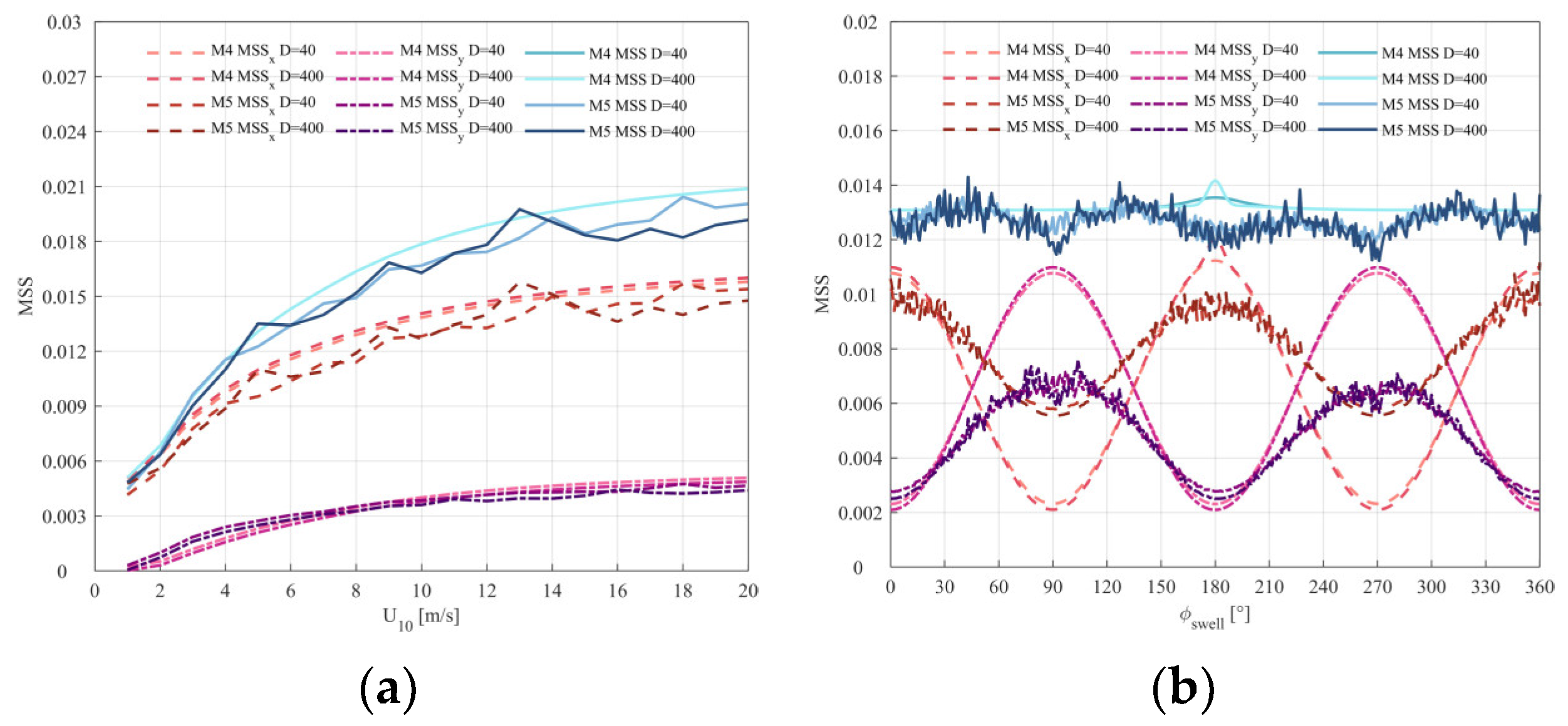
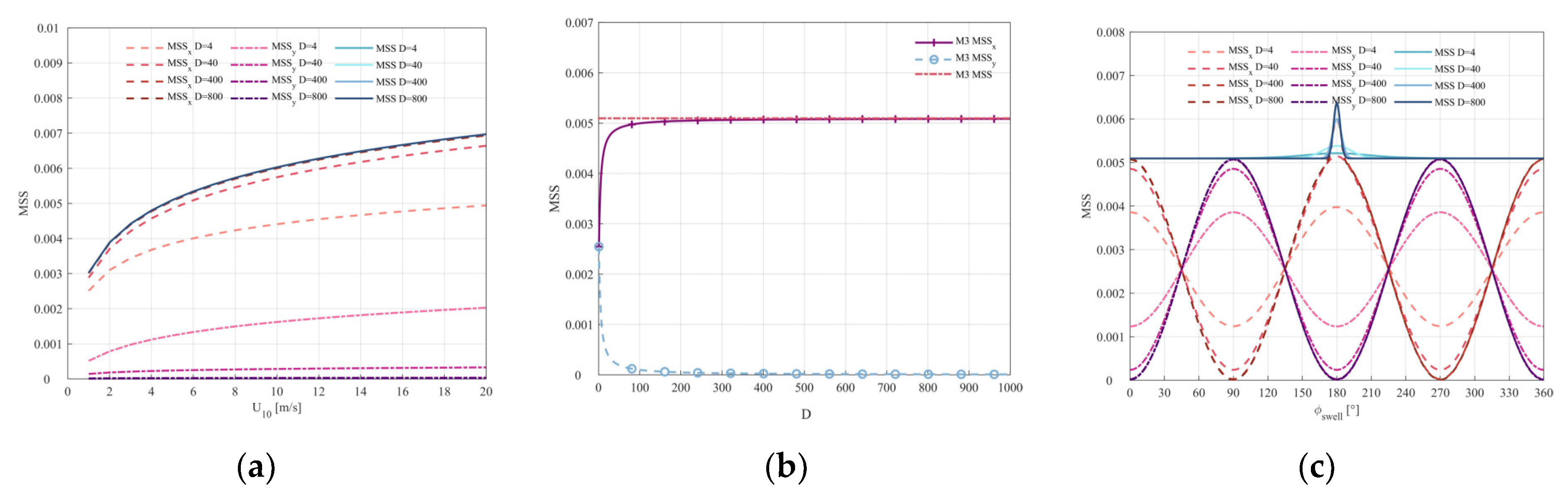
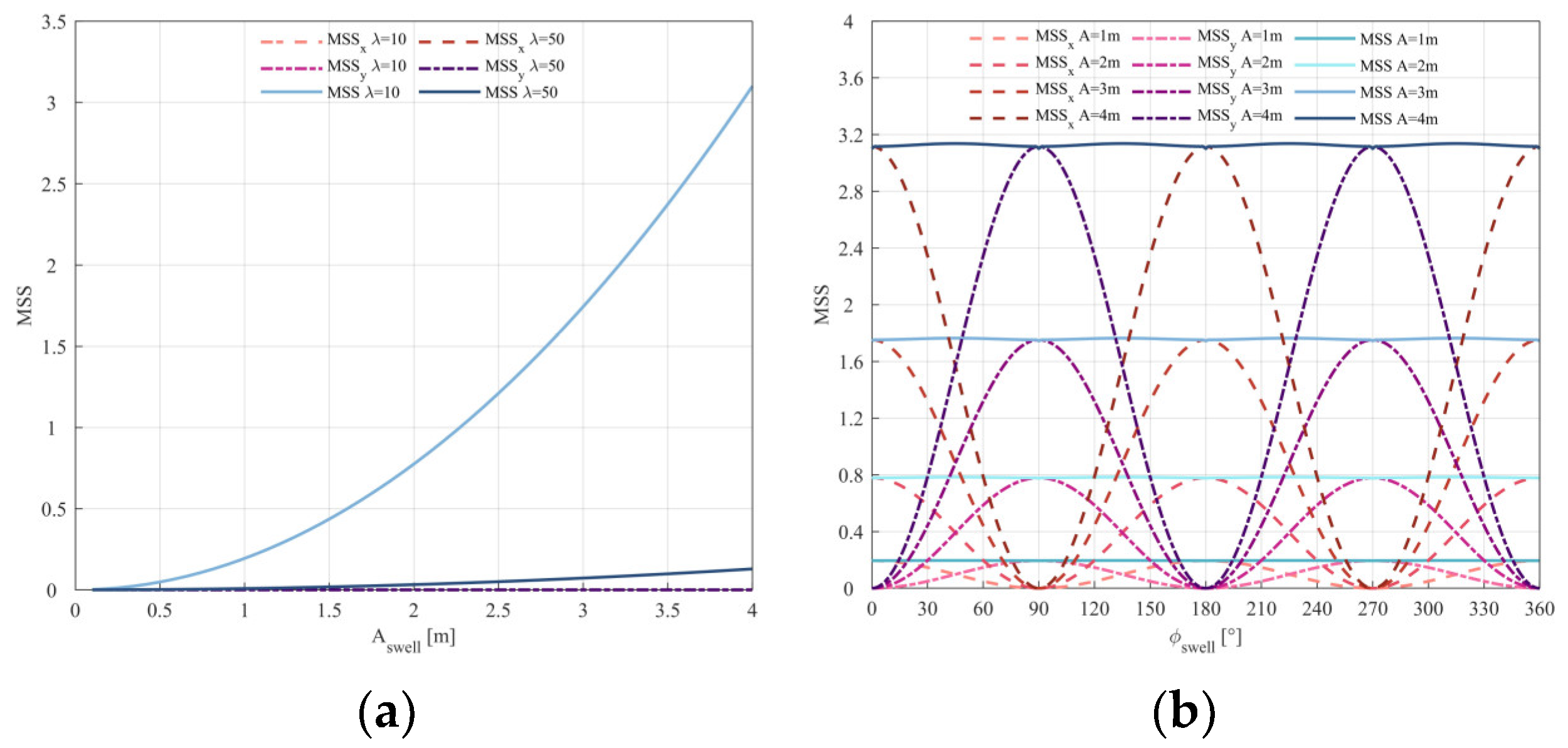
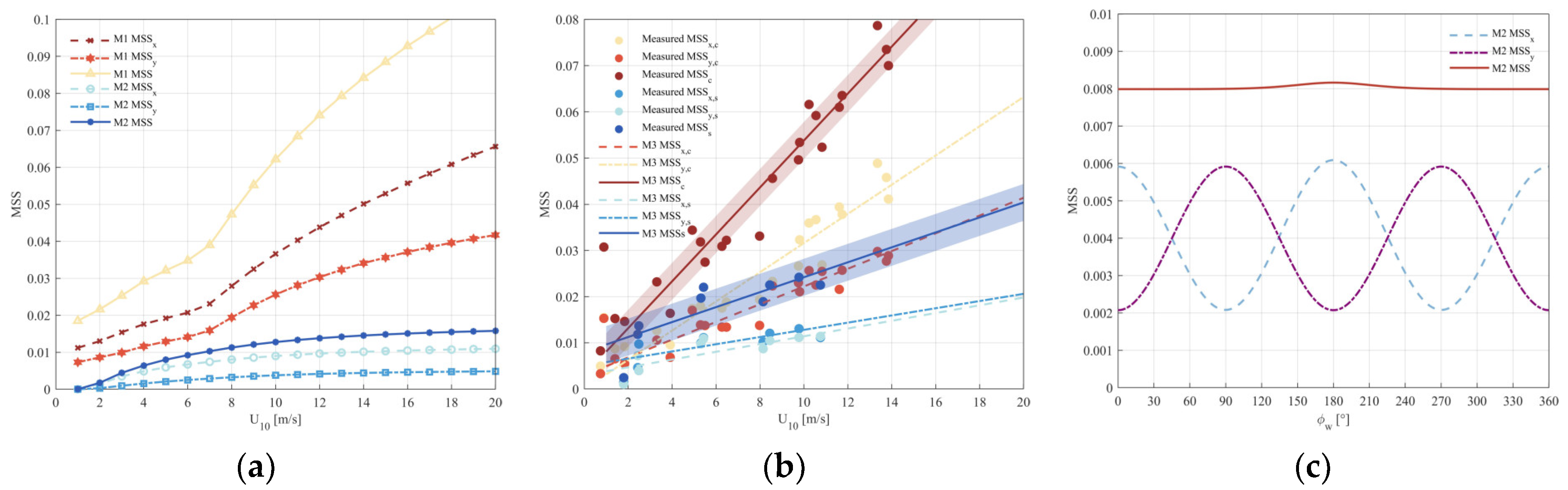
  • The results of various calculation methods of MSS on different kinds of sea surfaces have been analyzed, providing a solid foundation for the analysis of delay waveforms.
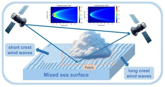
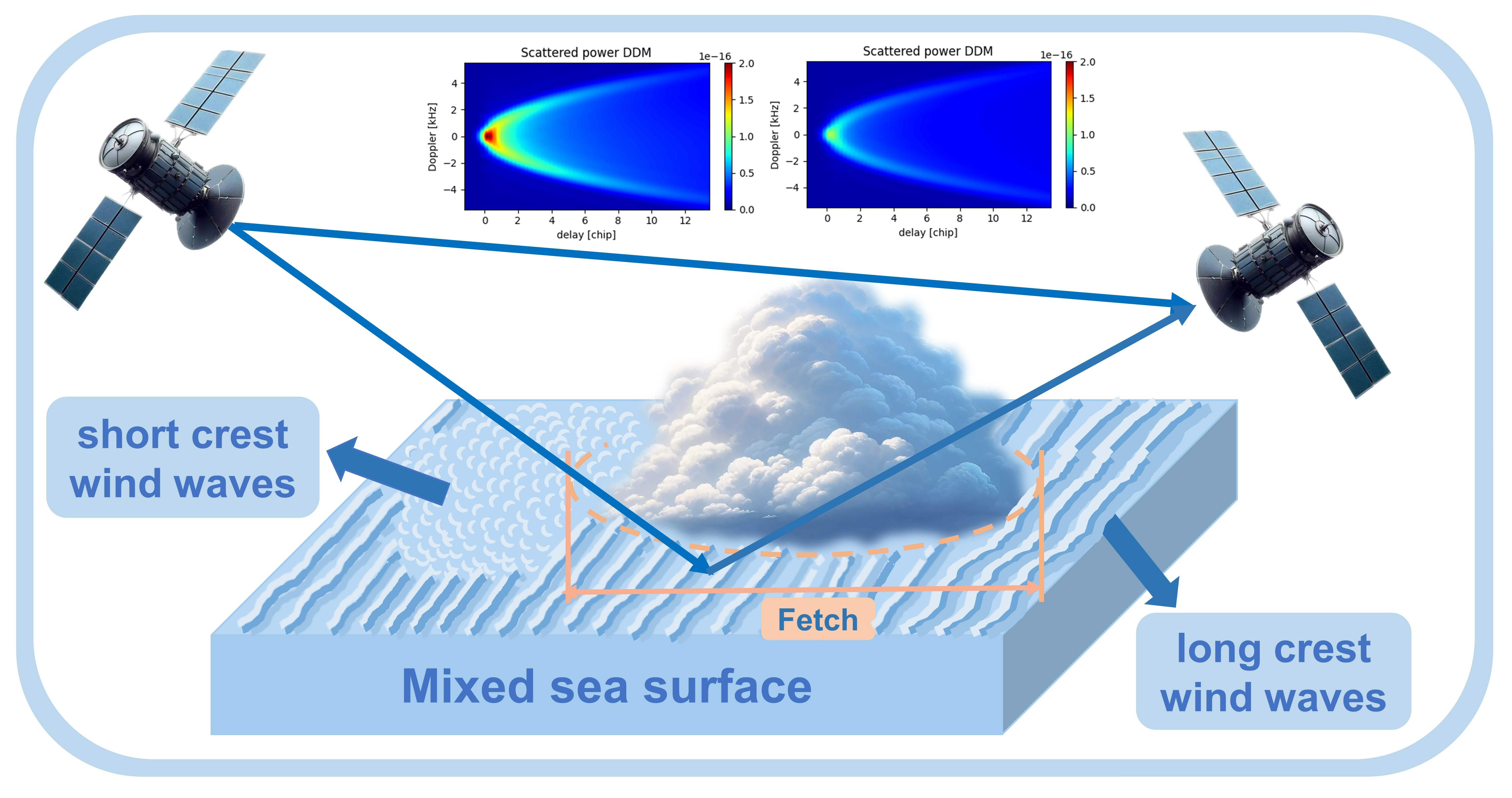
  • For the impact of multiple parameters on delay waveforms, some evident parameters such as directionality variables, direction of wave spreading, and others have been investigated comprehensively. As for different types of wind waves, the comparison and analysis of short-crest wind waves, long-crest wind waves, and mixed wind waves in the application of sea surface generation have been performed.
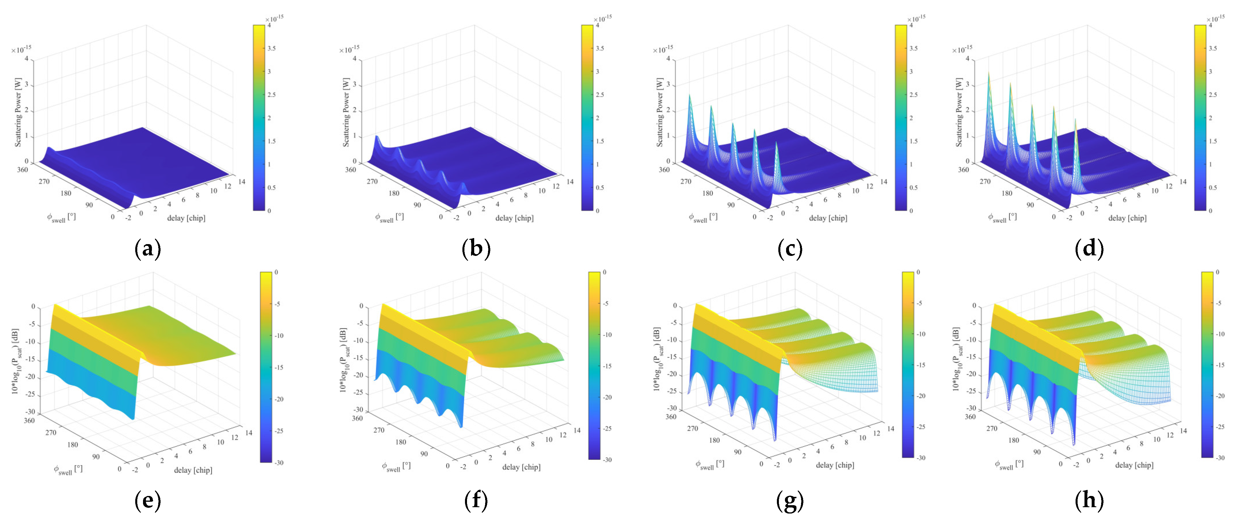
  • The impact of comprehensive parameters on the delay waveform on the basis of short-crest wind waves, long-crest wind waves, and mixed wind waves has been compared, predominantly illustrated to investigate the influence of short-crest wave components on the delay waveforms of a mixed sea surface.
Figure 1 is the flowchart of this paper, and the work presented in this paper mainly focuses on the univariate and joint influences of various parameters of monochromatic and mixed waves on delay waveforms. This paper is organized as follows: Section 2 briefly presents the theoretical background of GNSS-R, the realization of typical short-crest wind waves, and the influence of different wind speeds on delay waveforms. In Section 3, the detailed process for the impact of univariate and joint parameters on delay waveforms of long-crest wind waves is shown. Section 4 mainly presents the impact of multiple parameters on delay waveforms of a mixed sea surface combined with 2-D sinusoidal long-crest waves and short-crest components, predominantly studying the delay waveforms impacted by joint parameters such as wave amplitudes, wave length, and wave directions. Section 5 is devoted to the conclusions of this paper.

2. Impact of Multiple Parameters on Typical Wind Waves

Commencing with the derivation of the GNSS-R theoretical foundation and the comparison of real DDM and simulated DDM data, different parameters of wind sea surfaces and their characteristics represented as delay waveforms in the Z-V model have been researched in detail.

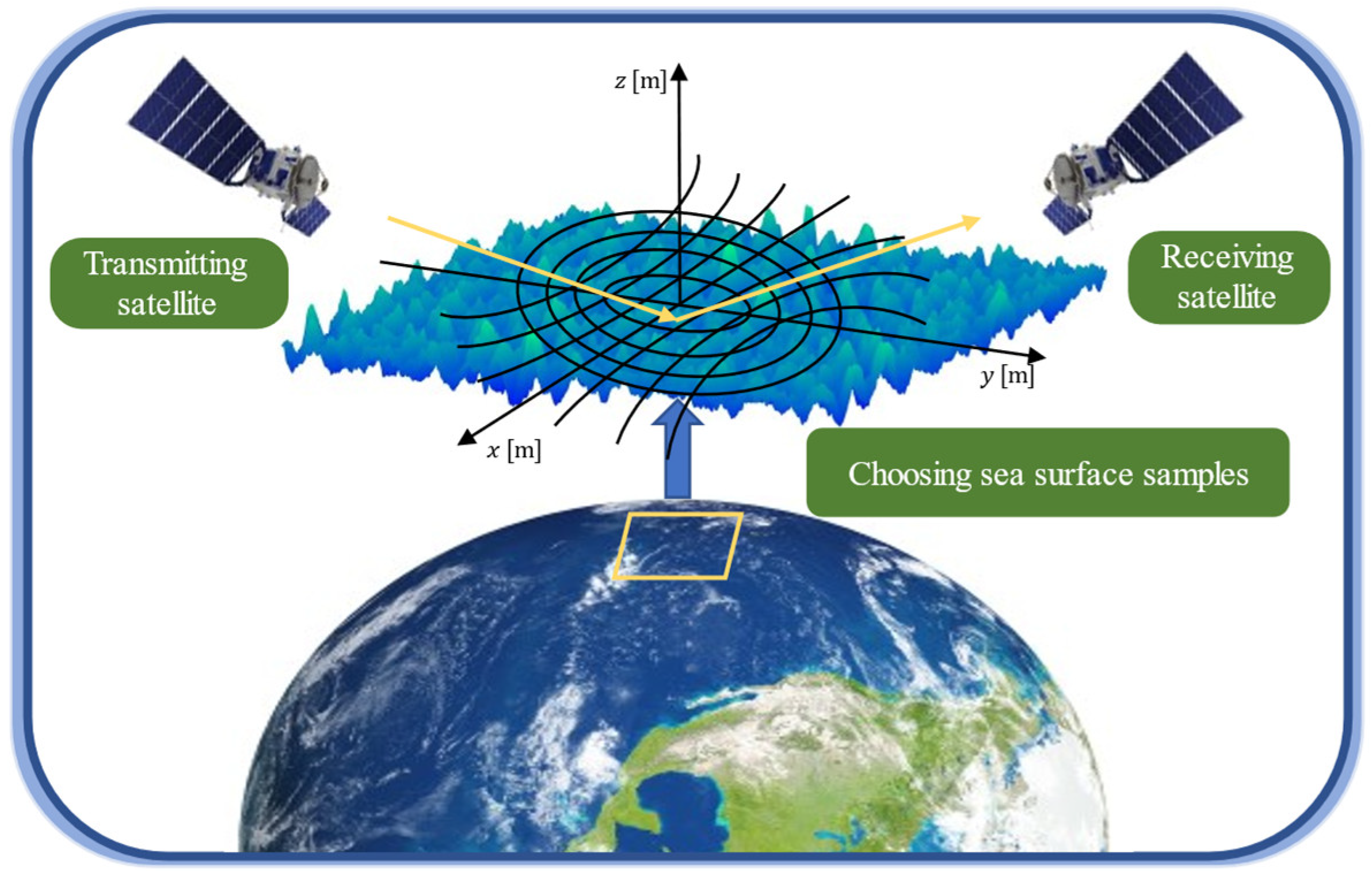
2.1. Theoretical Foundation of GNSS-R

The calculation of the MSS of the sea surface is the foundation and also an important procedure in the program of simulating the bistatic scattering model in the GNSS-R configuration; some MSS theories and results are set out in Appendix A. The famous Z-V model is widely applied in this area, and the derivations are exhibited as follows [26]:
< P s c a t τ , f c 2 > = χ 2 τ , f c P 0 τ , f c
The variable Pscat is the scattering power of the DDM, which is processed by taking P0 to convolve with the WAF (Woodward function). P0 is the scattering power which is not filtered by the WAF in two dimensions (delay range and Doppler range), much more specifically showing the contribution of each cell in the x-y area than Pscat. The expressions of the WAF function and P0 are provided in the following context:
χ 2 τ , f c = Λ 2 ( τ ) S f c 2
where Λ(τ) is the λ function that is decided by the C/A code:
Λ ( τ ) = 1 | τ | T c , τ T c 0 , τ > T c
Tc is the local pseudo-random code chip width. S(Δf) is the sinc function, defined as follows:
S ( Δ f ) = sin π × Δ f × T i π × Δ f × T i e j π × Δ f × T i
Ti is the coherent integration time. Additionally, the scattering power should be filtered by Λ(τ) and S(Δf) along the delay direction and Doppler direction, respectively:
P 0 τ , f c = P T λ 2 T i 2 ( 4 π ) 3 S G T ρ G R ρ σ mn 0 ρ R T 2 R R 2 δ τ τ ρ δ f c f d ρ d 2 ρ
In this equation, P0(τ, fc) is the incoherent scattering power because the following simulative examples are based on a sea surface with roughness, PT is the transmitted scattering power from a spaceborne transmitting satellite, and GT(ρ) and GR(ρ) refer to the transmitter’s antenna gain and receiver’s antenna gain, respectively, which are also chosen as a constant value of about 1.0. RT and RR are the distances from the transmitter and receiver to the scattering cell on the sea surface, respectively, σ mn 0 (ρ) is the scattering coefficient of each cell calculated by the KA-GO scattering model, and mn is the serial number of the sea-surface patch. The derivation of KA-GO is as follows:
σ 0 = π | R | 2 | q | q z 4 P q q z
where R is the Fresnel coefficient; q is the scattering vector of each cell; qz is the component along the z-direction of |q|; and P(−q/qz) is the probability distribution function (PDF), exhibited as follows [27]:
P q q z = e 1 2 ξ 2 + η 2 2 π σ u σ c × { 1 c 21 2 ( ξ 2 1 ) η c 03 6 ( η 2 3 ) + c 40 24 ( ξ 4 6 ξ 2 + 3 ) + c 22 4 ( ξ 2 1 ) ( η 2 1 ) + c 04 24 ( η 4 6 η 2 + 3 ) }  
where
ξ = q x / q z σ u ,   η = q y / q z σ c
c 21 = 0.01 0.0086 w s , c 03 = 0.04 0.0330 w s
c 40 = 0.40 ,   c 22 = 0.12 ,   c 04 = 0.23 .
σu refers to MSSx, and σc refers to MSSy.
Figure 2 is the configuration of GNSS bistatic scattering model, it describes the basic elements of the GNSS-R technique in spatial domain, introducing the relative location between the transmitting and receiving satellites. In the area composed of the black elliptical lines which represent the isochronous equal delay rings and the black hyperbola lines which represent the equal Doppler lines, it had been widely known that the majority of the scattering contributions come from this region, in which is named as “scintillation region”.
Figure 3 compares the real DDM with the simulated DDM of UK-DMC and CYGNSS in normalized form. The similar characteristics of the real and simulated DDM are the scattering power, with almost the same coverage near zero chip and zero Doppler shift, as well as the asymmetry of the axis at the zero Doppler position, which is parallel to the delay direction. The characteristics exhibited in Figure 3b,d with a wider bright coverage in the right area also apply to the real DDM in Figure 3a,c.

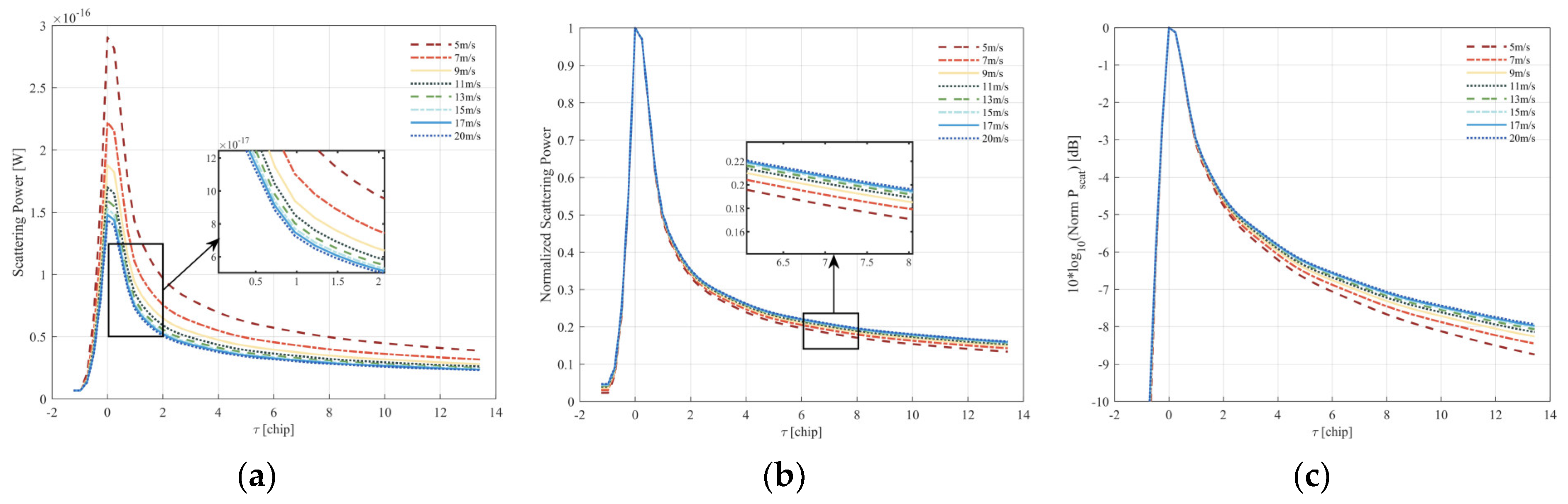
2.2. Impact of Wind Speed on Delay Waveform

Figure 4 displays the simulations of a typical short-crest wind sea surface under different wind speeds U10 and directions. Figure 4a,b show shorter extensions of the wave crests than in Figure 4c,d, which show larger extensions of the wave crests under the control of wind speed. The directions of wind waves exhibited isotropic characteristics within the justification of ϕw.
The results in Figure 5 are the simulated unnormalized and normalized scattering power in different wind speed conditions, and the curves are acquired by choosing the profile of the DDM at zero Doppler frequency shift, namely the delay waveform. The results reveal the reality that different wind speeds lead to a change in the peak power of delay waveforms; the higher the wind speed is, the lower the peak power will be. It is for this reason that the increase in MSS gives rise to the roughness of the sea surface so that the diffuse scattering of all contributed patches is enhanced, which causes a decrease in the total bistatic scattering power of the entire sea surface. Under the condition of low wind speeds, whether considering normalized scattering power or unnormalized scattering power, the discrepancy in the curves for different wind speeds is high enough so that the detection of wind speed will be efficient. However, the discrepancy in the higher wind speed comparatively decreases, which can be seen in Figure 5b,c, displaying that the curves of high wind speed cannot be distinguished clearly compared to a lower wind speed. The same conclusion was drawn by [29].
However, the trial edges of delay waveforms have not very obvious differences in various wind directions, which means that the detection of various wind directions on the basis of typical short wind waves by means of simply distinguishing trial edges is not feasible.

3. Impact of Multiple Parameters on Long-Crest Wind Waves

In the above section, the background of GNSS-R, a comparison of a real DDM and simulated DDM along with the impact of wind speed on delay waveforms was performed. In this section, we will predominantly focus on the aspect of the influence of multiple parameters on long-crest wind waves, calculate the MSS under various parameters, compare the delay waveforms of different wave directions, and finally find the conspicuous characteristics.

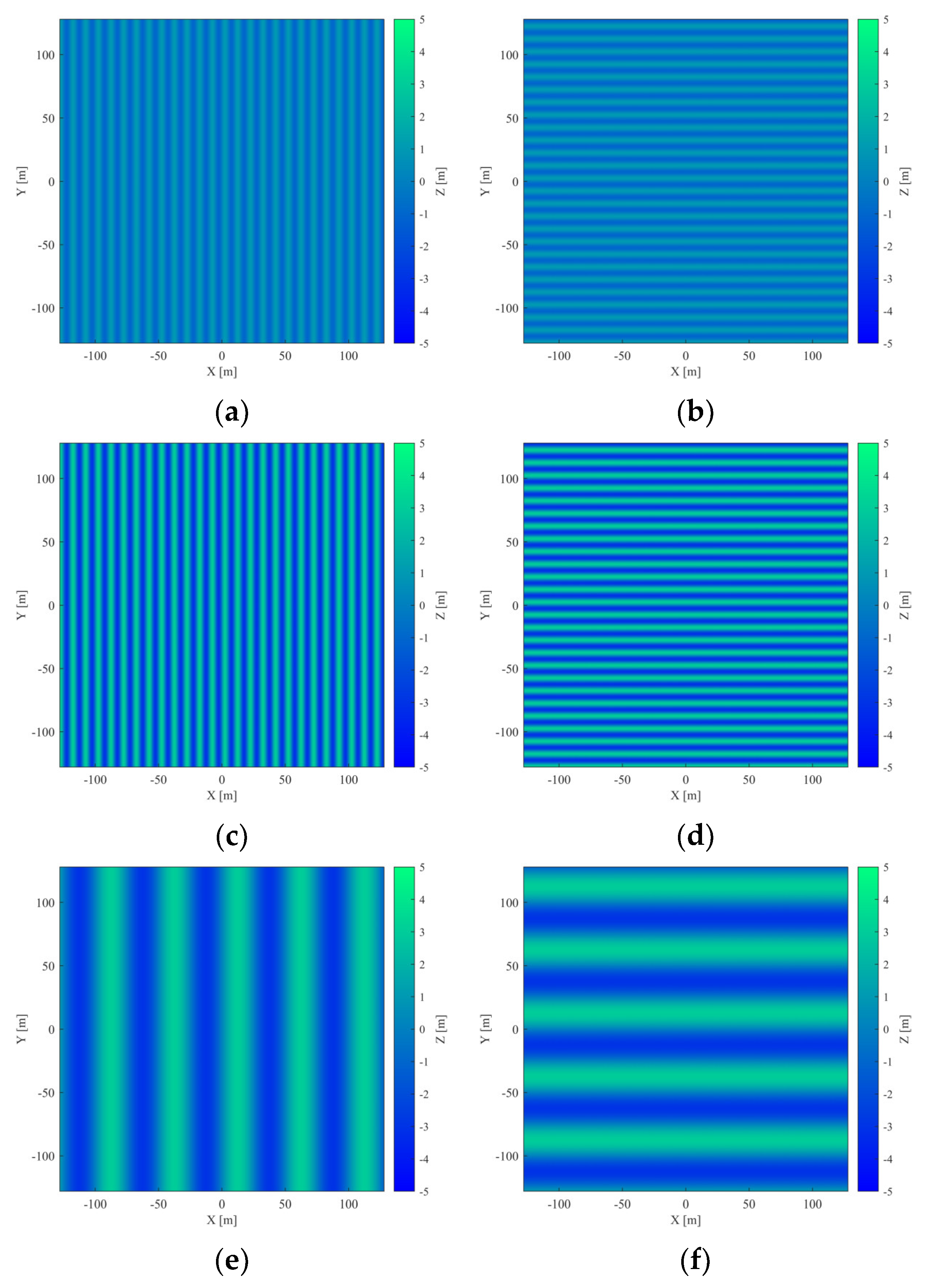
3.1. Long-Crest Wind Sea Surface

The typical sea surface also can be simulated by filtering the 2-D power spectrum, made up of the JONSWAP spectrum and spreading function, which are derived as follows:
S ( k ) = 1 k Ψ JONS ( k ) Φ ( k )
where the function ΨJONS(k) originates from ΨE(k), which is called the Elfouhaily spectrum, and the derivation of ΨJONS(k) is as follows:
Ψ JONS ( k ) = α p 2 k 3 L PM J P
The generalized equilibrium range parameter αp = 4 × 10⁻³, LPM = exp[−(1.25(k/kp)−2)]; Jp = γB, and the constant γ = 10. The specific values of αp and γ can make the sea surface exhibit characteristics of long-crest wind waves [30]. As for the spreading function Φ(k), the most popularly used function is the Longuet-Higgins angle distribution function:
Φ LH ( k , ϕ ) = G ( D ) cos ϕ ϕ w 2 2 D
G ( D ) = 1 / π π cos 2 D φ 2 d φ
In this equation, G(D) is a function of the directionality variable D which can be changed, and ϕw denotes the direction of wind waves.
Using a linear filtering method, the height of each location can be represented as follows:
Z ( r , t ) = F 1 [ A ( k , t ) ] = k A ( k , t ) exp ( j k r )
where F−1[…] refers to the symbolic expression for the inverse Fourier transform, and A(k, t) denotes the complex amplitude of the frequency domain:
A ( k , t ) = Y ( k ) * S ( k , π φ ) Δ k x Δ k y exp ( j ω t ) + Y ( k ) S ( k , φ ) Δ k x Δ k y exp ( j ω t )
Y(k) is a complex Gaussian random sequence, and Δkx and Δky denote the interval of frequency along the x direction and y direction, respectively. However, by choosing a specific αp and γ as well as altering the value of the directionality parameters D, the crest will transform from short scale to long scale. The different sea surface samples with various directional variables D and wind speed U10 are showed as follows in Figure 6.
Figure 6 depicts the sea surface filtered by parameters adjusted with the JONSWAP spectrum within the conditions of different U10, D, and ϕw. Table 1 shows the parameters of simulated waves in Figure 6 and the significant wave height he (SWH). This group of surfaces shows different kinds of wind waves, which also provide characteristics closer to an optical image.
After comparing Figure 4a with Figure 6a, we find that the waves in Figure 6a comparatively lack the finer details, which can be easily tracked in Figure 4a. This indicates that the wind waves (Figure 4a) contain more dense small-scale waves than those presented in Figure 6a. When the wave grows with more concentrated directionality, the characteristics of an increasing scale of wave crest developed, just as Figure 6b shows.
Focusing on Figure 6c,d, the concentration of wave spreading direction becomes stronger with the increase in directionality variables D, and the scale of the wave crest also increased with the increase in D. The comparison between each plot in Figure 6 clearly displays the distinct effect of wind speed, wave direction, and directionality on wind waves: wave direction dominates the spreading direction of wind waves, while directionality parameter D decides the concentration of the wave spreading direction and the crest scale of wind waves.
Figure 7 shows the results of MSS calculated by M2, which is specifically introduced in Appendix A. Figure 7a is the result of the MSSx, MSSy, and MSS of different directionality parameters D, revealing that MSSx and MSS persistently increase with U10, but the MSSy does not always increase; especially for the cases where D is greater than 4, the MSSy seems insensitive to an increasing D. This is because the MSSx, MSSy, and MSS results of Figure 7a are calculated under the condition of ϕw = 0°, in which case the wave fluctuation as well as the MSS along the y-axis direction will be weak.
It can be clearly seen from Figure 7b that in the region of D approximately below 250, the higher the D is, the smaller the MSSy will be. When the value of D is large enough, the spreading direction of wind waves will become concentrative enough. By contrast, the MSSy will tend to be zero, as shown by the curve of the dot–dash line with a blue color. The MSSx and MSSy exhibit the anti-phase changing regulation with wave directions.

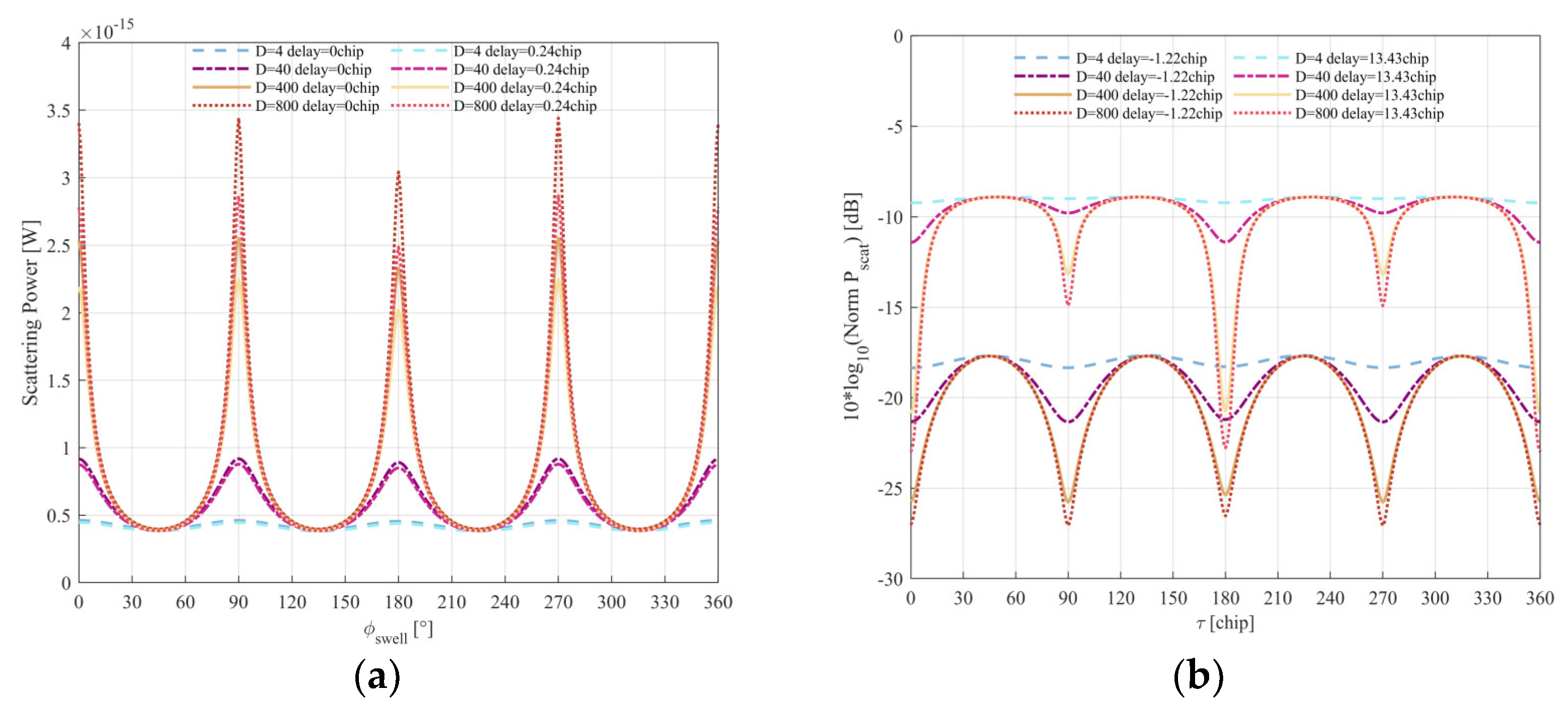
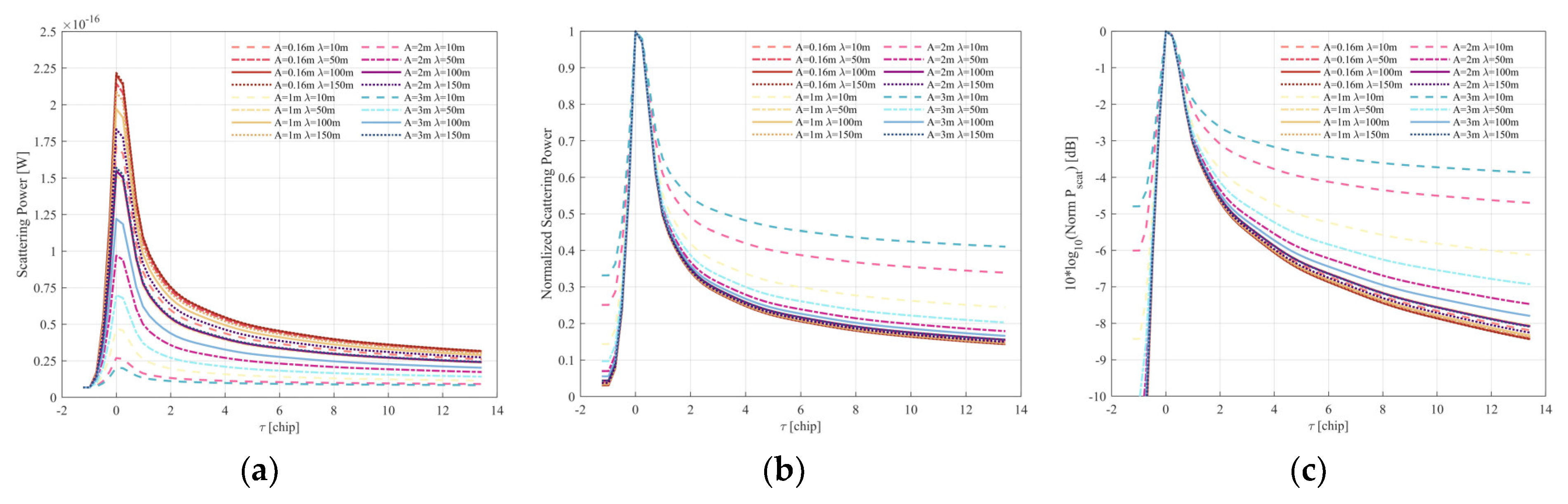
3.2. Joint Influence of Parameters on Delay Waveforms of Wind Waves

Figure 8 displays some results for delay waveforms, aiming to investigate the directionality variable D, how it impacts delay waveforms, and how it influences trial edges within different U10 for short- and long-crest wind waves. As for Figure 8c, it originates from the normalized scattering power shown in Figure 8b but has a more obvious margin between different curves. It is always used to obtain the inversion of wind speed from the trial edges of curves. But for cases of the same U10 with different D, Figure 8c unveils a previously undisclosed aspect that different curves have obvious differences. Then, we can draw the conclusion that the trial edges of normalized delay waveforms can be a potential tool for detecting the directionality of wind waves. Moreover, we can also notice that with the increase in the directionality parameter D, the margins between two lines corresponding to different U10 become smaller, so an increasing D will deteriorate the detectability of wind speed. The directionality parameter D not only has influence on the inversion of U10 but also impacts the detection of the directions of wind waves; some evident characteristics also emerge in the following Figure 9.
Figure 9 provides a relatively impressive perspective on the impact of directionality on detecting the direction of wind waves. For Figure 9a, D = 4 and U10 = 5 m/s, the delay waveform of each direction reveals that the peak power close to the zero chip almost does not fluctuate along the increasing wave direction. This was demonstrated in the above text, and the same conclusion can be drawn that the distinction of the spreading direction of short-crest wind waves (because D = 4 corresponds to short-crest wind waves) cannot be accomplished only by the trial edges or peak scattering power under the configuration of pure specular scattering, the KA-GO scattering model, or polarization, which was suggested by Camps et al. [19] and Zhang et al. [25].
From a macro point of view, each 3-D surface in Figure 9b–d has five peak values at 0°, 90°, 180°, 270°, and 360° and four valley values at 45°, 135°, 225°, and 315°. This characteristic can be included as a periodical fluctuation near zero chip. Figure 9e–h are processed by “dB”; the fluctuation along the direction of wind waves near −1.22 chip and 13.43 chip show the property of periodical fluctuation. For the purpose of comparing these two profiles, the results in Figure 10 will be carefully analyzed.
Figure 10 shows the profile from Figure 9 along the wind direction ϕw. Figure 10a displays that the increase in D leads to the peak values and sub-peak values becoming larger; however, the valley values almost do not change. Therefore, the largest margin between the peak values and valley values would be achieved for the case of D = 800, which can be named as long-crest wind waves, and also close to the 2-D sinusoidal long-crest wind waves in the following simulation in Section 3.3. Moreover, the “U”-type curves for 0 chip have greater peak values than the curves for 0.24 chip.
Figure 10b presents the profiles near −1.22 chip and 13.43 chip. With the increase in D, the fluctuation of the curves near −1.22 chip and 13.43 chip becomes drastic, leading to the conclusion that the increasing predominance of long-crest wind waves (increasing D) makes directional recognition easier. Comparing the curves near −1.22 chip and 13.43 chip, it can be noted that the curves near 13.43 chip have the lowest or sub-lowest value, different from the curves near −1.22 chip, which have almost the same lowest value. The above comparison indicated that the fluctuating curves near 13.43 are more appropriate for directional inversion rather than the curves near −1.22 chip.

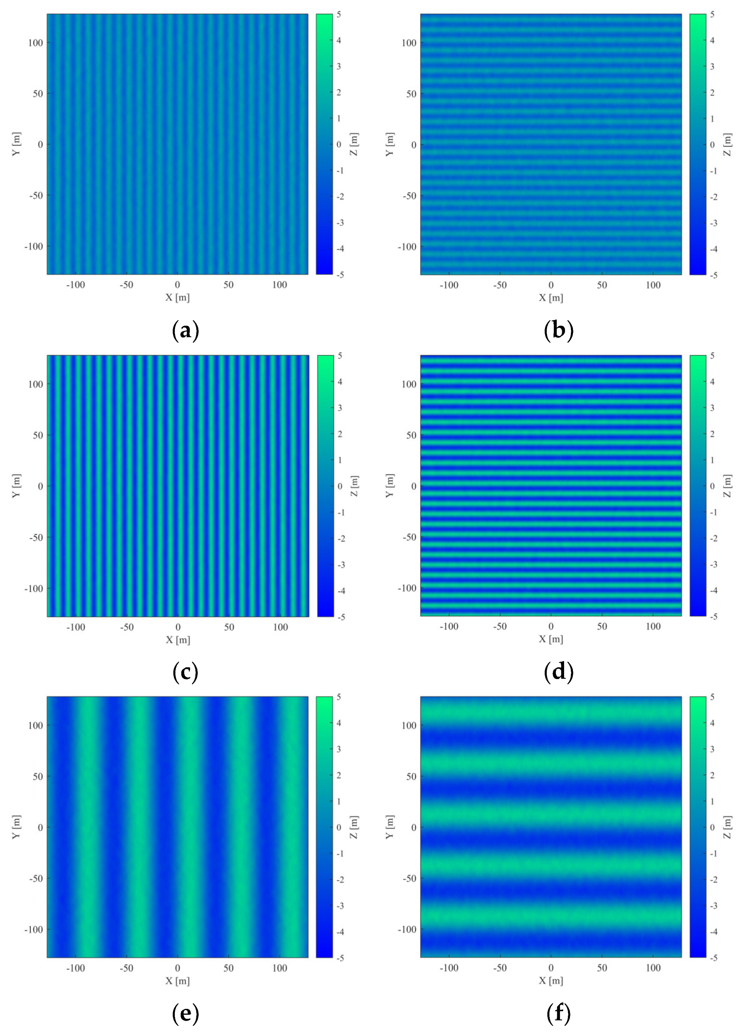
3.3. 2-D Sinusoidal Wind Sea Surface

Although the wind sea surfaces simulated above are realistic representations of the real sea surface, the wave height of wind waves is decided by the U10. However, once the U10 changed, not only did the wave height change but the wave length was also altered simultaneously. In consideration of this reason, using wind waves filtered by a traditional power spectrum is not appropriate for simulatively investigating the impact of multiple parameters on delay waveforms. To facilitate univariate manipulation, the 2-D sinusoidal function is substituted for the wind wave spectrum because of its flexibility in modulating parameters like the amplitude, wave vectors and wave length, or others. The following results show the absolutely long-crest wind waves and the impact of multiple parameters influencing the MSS and delay waveforms.
Figure 11 displays the 2-D sinusoidal long-crest wind sea surface under different amplitudes, directions, and wave length. The texture characteristics coincide with the parameter settings. Because artificially truncating the upper limit of the integral (M2) is not appropriate for the discontinuous-spectrum sea surface, the iterative method of facets (M5) is used to calculate the MSS in the following results.
Figure 12a shows that the MSS and its components rise with an increasing A. The curves of MSSx and MSSy in Figure 12b both exhibit periodicity and have a similar change trend to that in Figure 7c. The influence of the wave height on the delay waveforms with the increase in ϕw will be investigated in the following part.

3.4. Joint Influence of Parameters on Delay Waveforms of 2-D Sinusoidal Wind Waves

Comparing Figure 13a,b, we can see that the peak value decreases with the increase in the wave amplitude because the increasing amplitude gives rise to the increasing roughness of the wind sea surface. Comparing Figure 13a with Figure 9d, it should be noted that the amplitude of the 2-D sinusoidal wind wave is 0.4 m, and its significant wave height (SWH) is about 0.8 m, which is close to the SWH of Figure 6c. What is more, the sectional view of waveforms along the direction of ϕw is similar, but the peak values of the two figures are different. It is indicated that the curve value decreases faster around the peak value than that in Figure 9d, for the reason that the simulated absolutely long-crest wind waves of the 2-D sinusoidal spectrum contain much more concentrative spreading waves, while the spreading directions of the simulated wind waves are not concentrative enough for the large D case (D = 400). Figure 13c,d exhibit the detectable trail edges of waveforms with increasing ϕw. It can be noticed that the values along the direction of ϕw near 0 chip are always zero dB, but the sectional curves near −1.22 chip and 13.43 chip still exhibit an obvious property of periodical fluctuation. From this fact, the sectional curves near −1.22 chip and 13.43 chip can also provide a foundation for the detection of ϕw.
The above analysis demonstrated the validity of the substitution from wind waves filtered from a traditional spectrum to 2-D sinusoidal long-crest wind waves in three aspects: SWH, the MSS, and delay waveforms. It can be concluded that 2-D sinusoidal wind waves have many advantages in the application of univariate investigation. Next, the impact of multiple parameters on a mixed sea surface has been investigated in detail.

4. Impact of Multiple Parameters on Mixed Sea Surface

Considering the inflexibility of univariately controlling the parameters of wind waves filtered by a traditional spectrum, we find that simulation based on a comparatively real physical mechanism is especially important. The following context investigates the multiple parameters impacting delay waveforms under a mixed sea surface combining 2-D sinusoidal large-crest wind waves with short-crest wind waves.

4.1. Mixed Sea Surface

The above simulations of a mixed sea surface are simulated under different conditions of amplitude A and λ, which show obvious textured characteristics originating from a 2-D sinusoidal function. The difference between Figure 12 and Figure 14 is that the surfaces in Figure 14 present more short-crest waves. Because the real wave height of wind waves with superimposed short-crest waves is commonly about 3~4 m, the amplitude of a mixed sea surface in this figure is settled as 1 m, 2 m, and 3 m, which makes the results more informative.

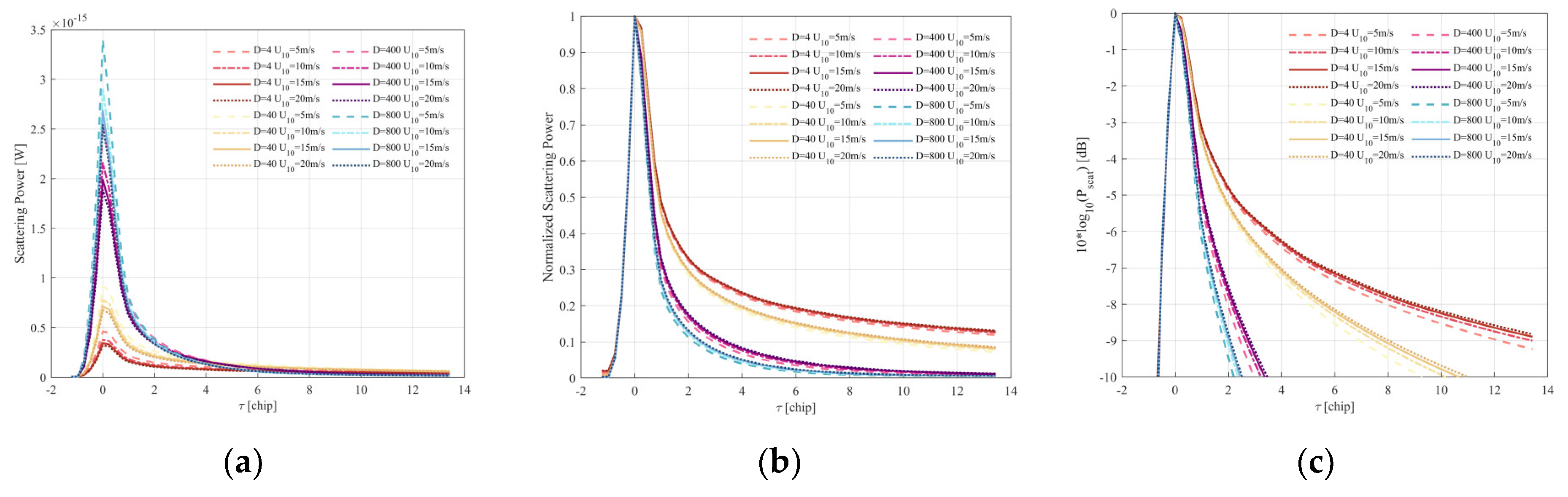
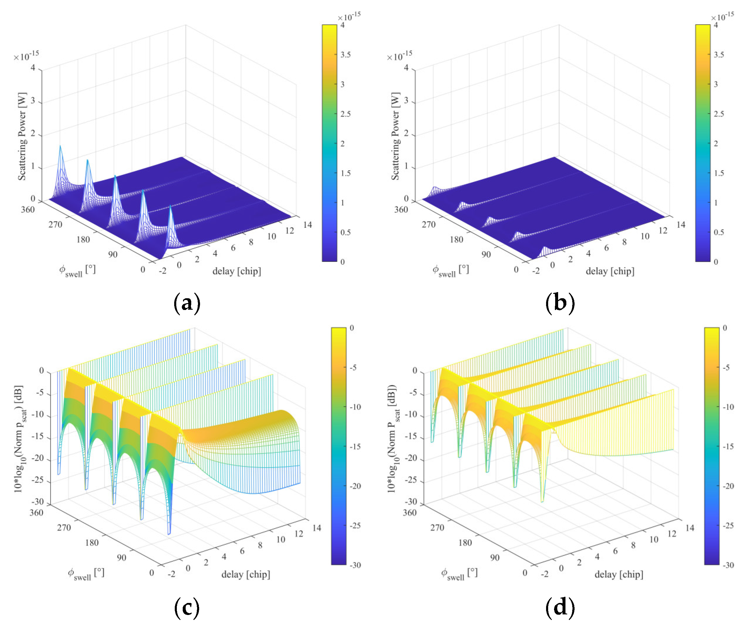
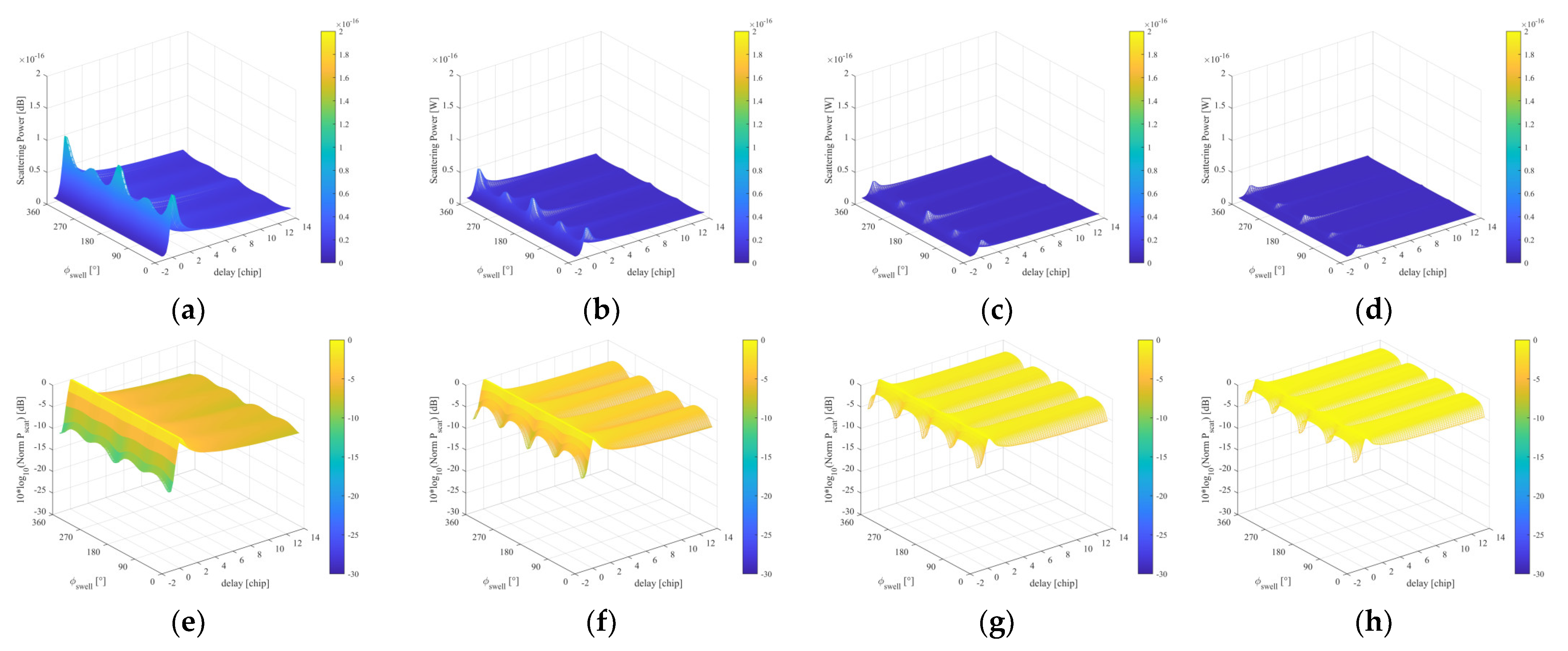
4.2. Joint Influence of Parameters on Delay Waveform of Mixed Sea Surface

Taking notice of the peak value near zero chip in Figure 15a, it can be observed that the lower value of λ results in an increase in the roughness and the MSS, which leads to a decrease in the scattering power. Moreover, comparing the curves with the same λ and different amplitude A, it can be observed that the scattering power decreases with the increase in the amplitude of wind waves. The larger the λ and A are, the faster the decrease rate of the trial edges will be, which is shown clearly in Figure 15c.
The results in Figure 16 originate from the calculation of the MSS on a mixed sea surface (2-D sinusoidal long-crest wind waves with Elfouhaily short-crest wind waves) by M5, which is slightly different from M4, and both of these two methods are introduced simply in Appendix A. Comparing Figure 13a and Figure 16a, we can find that the sectional curve near zero chip also shows the property of periodical fluctuation, and the rate of the decrease in the curve near the peak value of the former is smaller than that of the latter. The reason for this situation is that Figure 16 shows long-crest wind waves with short-crest wave components, while Figure 13 only shows pure long-crest wind wave components. The short-crest wind wave components give rise to the roughness of the sea surface, also impeding the decreasing rate of sectional curves around the peak value. As for Figure 16b–d, with the increase in wave amplitude, the total scattering power decreases, and the rate of the decrease near the peak value becomes larger. Last but not least, when the wave length increases but other parameters are fixed, the delay waveform does not show much of a difference at different angles of long-crest wave directions. In a word, the A and ϕw of long-crest waves play a comparatively more significant role in the joint influence of multiple parameters on the delay waveforms of the mixed sea waves.

5. Conclusions

This paper investigates the influence of multiple parameters of mixed sea waves on the delay–Doppler map (DDM) in GNSS-R from various aspects: wind speed parameters, typical wind wave parameters, and 2-D sinusoidal wind wave parameters, as well as their counterparts in mixed-wave conditions. The simulated DDMs are verified via comparison with measured data. Then, the characteristics analysis is performed based on the proposed methods. Some conclusions can be drawn as follows:
Firstly, the trial edges of delay waveforms presenting captured characteristics such as the trial edges of slope vary greatly at different wind speeds.
Secondly, a comparison between the results of wind sea surface and mixed wind sea surface was performed. The mixed wind sea surface contains long- and short-crest wave components, indicating that the short-crest wind wave components play a nonnegligible role in the sectional profiles of 3-D delay waveforms.
Finally, the delay waveforms along the direction of wind waves show the property of periodical fluctuation near 0 chip as well as −1.22 chip and 13.43 chip. Moreover, with an increase in wave height, the total scattering power decreases, and the rate of decrease near the peak value becomes higher.
The work presented in this paper provides a solid theoretical foundation for the inversion of wind speed and wind direction in the sea with complicated wind components.

Author Contributions

Conceptualization, D.N.; methodology, J.Y. and D.N.; software, D.N., J.Y. and K.Z.; validation, J.Y. and D.N.; formal analysis, J.Y.; investigation, J.Y. and K.Z.; resources, D.N. and J.Y.; data curation, J.Y.; writing—original draft preparation, J.Y.; writing—review and editing, D.N. and M.Z.; visualization, J.Y.; supervision, D.N.; project administration, D.N.; funding acquisition, D.N. All authors have read and agreed to the published version of the manuscript.

Funding

This research was funded by the 111 Project (Grant No. B17035), the Natural Science Basic Research Program of Shaanxi (Grant No. 2023-JC-YB-543), the Aeronautical Science Foundation of China (Grant No. 2022Z017081007), and the Fundamental Research Funds for the Central Universities.

Data Availability Statement

Data is contained within the article.

Acknowledgments

We would like to thank the anonymous reviewers for providing invaluable and constructive comments and suggestions.

Conflicts of Interest

The authors declare no conflicts of interest.

Appendix A

The Appendix introduces several methods of calculating the MSS, which are appropriate for different sea surface scenarios. Taking the advantages and disadvantages of these methods into consideration, the feasibility will be analyzed from two aspects: MSS theoretical and results analysis.
There are multiple methods of calculating the MSS of the sea surface (see Figure A1), such as using the equation derived from Elfouhaily and truncating the upper limit of the integral system (M2) or not (M1), as well as using the conclusions from Cox–Munk model, which is subsequently referred to as Method 3 (M3). The results of Method 1 and Method 2 for the calculation of the MSS changing with the increase in wind speed are as depicted in Figure 3a. Elfouhaily first proposed Method 2 and derived the equations as follows [31]:
M S S x = π π k 2 cos 2 ϕ Ψ ( k , φ ) d k x d k y
M S S y = π π k 2 sin 2 ϕ Ψ ( k , φ ) d k x d k y
M S S = M S S x + M S S y = 0 k 2 S ( k ) d k
Method 1 strictly obeys the above equations using an antiderivative, and the up-limit of the integral is over 2000 or more. Method 2 also uses the same equation, but the up-limit of integral is smaller by about 3.56 because of the known algorithm: kcut = 2πcosθicut, θi is the incidence, and λcut is a wavelength of about 0.6 m under the regime of a transmissive satellite of GNSS-R. Comparing Method 1 with Method 2, the results show that the values of MSSx and MSSy calculated with Method 1 are both higher than those calculated with Method 2 because of the different settings of Δk, kmin, and kmax. Moreover, the value of MSSx is always higher than that of MSSy in Figure A1, for the reason that the set direction of wind waves is parallel with the x-axis. Additionally, Figure A1b shows the results of MSS (M3) within the conditions of a clean sea surface and slice sea surface acquired with the Cox–Munk model [32]:
M S S clean = 5.12 × 10 5 U 10 + 0.003 ± 0.004
M S S slice = 1.56 × 10 5 U 10 + 0.008 ± 0.004
M S S x , c = 3.16 × 10 3 U 10
M S S y , c = 1.92 × 10 3 U 10 + 0.003
M S S x , s = 0.84 × 10 3 U 10 + 0.003
M S S y , s = 0.78 × 10 3 U 10 + 0.005
In Figure A1b, the scattering points in different colors are the measured data from Cox–Munk, and the different lines with error shadings are the fitting results corresponding to those scattering points. However, the MSS of the Cox–Munk model is not susceptible to wind direction, so the MSSx and MSSy cannot be acquired by using the Cox–Munk model.
Figure A1c describes the MSS of the wind sea surface under the condition of different wind directions, showing that the MSS of the wind sea surface fluctuates a little under the condition of various wind directions. Furthermore, the MSSx and MSSy exhibit anti-phase periodicity.
Figure A1. Three methods of calculating MSS: (a) Method 1 (M1) and Method 2 (M2) of calculating MSSx, MSSy, and total MSS; (b) Cox–Munk model of calculating MSSx, MSSy, and MSS; (c) MSSx, MSSy, and MSS changing with different ϕw under the condition of U10 = 5 m/s.
Remotesensing 16 01395 g0a1
Figure A2 displays a mixed sea surface combining long-crest wind waves with short-crest wind waves. Comparing Figure A2a with Figure A2b, we can observe that the directions of long-crest wind waves have changed. As for Figure A2a,c, with the increase in D, the spreading directions of long-crest wave components are more concentrative. The following M4 and M5 are applied to calculate the MSS results of these sea surface scenarios.
Figure A2. Simulations of mixed sea surface with long- and short-crest components under the condition of different D and ϕw. (a) D = 40, and ϕw = 0°; (b) D = 40, and ϕw = 90°; (c) D = 400, and ϕw = 0°; (d) D = 400, and ϕw = 90°.
Remotesensing 16 01395 g0a2
Figure A3 shows the comparison of MSS results calculated by M4 and M5. M4 is processed by superimposing the MSS results of short-crest waves on large-crest waves directly, which essentially originates from M2. M5 is a new method with great ease, the process of which can be derived as the following equations:
M S S x = i = 1 , j = 1 i = M , j = N ( Z 1 , 2 Z 1 , 1 x 2 x 1 ) 2 + ( Z 1 , 3 Z 1 , 2 x 3 x 2 ) 2 + + ( Z 2 , 2 Z 2 , 1 x 2 x 1 ) 2 + ( Z 2 , 3 Z 2 , 2 x 3 x 2 ) 2 + + ( M 1 ) × ( N 1 ) ( Z i , 2 Z i , 1 x 2 x 1 ) 2 + ( Z i , 3 Z i , 2 x 3 x 2 ) 2 + + ( Z M , N Z M , N 1 x N x N 1 ) 2 ( M 1 ) × ( N 1 )
M S S y = i = 1 , j = 1 i = M , j = N ( Z 2 , 1 Z 1 , 1 y 2 y 1 ) 2 + ( Z 3 , 1 Z 2 , 1 y 3 y 2 ) 2 + + ( Z 2 , 2 Z 1 , 2 y 2 y 1 ) 2 + ( Z 3 , 2 Z 2 , 2 y 3 y 2 ) 2 + + ( M 1 ) × ( N 1 ) ( Z 2 , j Z 1 , j y 2 y 1 ) 2 + ( Z 3 , j Z 2 , j y 3 y 2 ) 2 + + ( Z N , M Z N , M 1 y N y N - 1 ) 2 ( M 1 ) × ( N 1 )
M S S = M S S x + M S S y
Zij is the height data of grid location (i, j), xi is the abscissa data, and yj is the vertical axis data. M and N are the number of sampling points along the x axis and y axis, respectively. Focusing on Figure A3a, the MSS results increase with the intensification of U10, giving rise to the increasing roughness of the sea surface. It is also worthy to notice that the MSS calculated by M5 fluctuates in a limit range around the smooth curves calculated by M4. Consequently, the results of M4 can be seen as the fitting results of M5.
Figure A3b shows the changing trend of MSS with ϕw, which can be used to investigate the univariate and joint influence of ϕw and D on delay waveforms. MSSx and MSSy show anti-phase change with the increase in ϕw. Nevertheless, the MSSx and MSSy calculated by M5 do not overlap entirely; it can be explained that the long-crest wind waves are comparable to the short-crest wind waves. Additionally, the directionality variable D has a slight impact on the MSSx, MSSy, and MSS, so the two curves of different D are close, as shown in Figure A3b.
Figure A3. Comparison of MSS calculated by M4 and M5 for composite sea surface (superimposing short-crest waves on long-crest waves): (a) the MSS change with U10; (b) the MSS change with ϕw.
Remotesensing 16 01395 g0a3

References

  1. Jin, S.; Feng, G.; Gleason, S. Remote sensing using GNSS signals: Current status and future directions. Adv. Space Res. 2011, 47, 1645–1653. [Google Scholar] [CrossRef]
  2. Yu, K.; Rizos, C.; Burrage, D.; Dempster, A.G.; Zhang, K.; Markgraf, M. An overview of GNSS remote sensing. EURASIP J. Adv. Signal Process. 2014, 2014, 134. [Google Scholar] [CrossRef]
  3. Edokossi, K.; Calabia, A.; Jin, S.; Molina, I. GNSS-reflectometry and remote sensing of soil moisture: A review of measurement techniques, methods, and applications. Remote Sens. 2020, 12, 614. [Google Scholar] [CrossRef]
  4. Vaquero-Martínez, J.; Antón, M. Review on the role of GNSS meteorology in monitoring water vapor for atmospheric physics. Remote Sens. 2021, 13, 2287. [Google Scholar] [CrossRef]
  5. Yu, K. Theory and Practice of GNSS Reflectometry; Springer: Berlin/Heidelberg, Germany, 2021. [Google Scholar]
  6. Jin, S.; Wang, Q.; Dardanelli, G. A review on multi-GNSS for earth observation and emerging applications. Remote Sens. 2022, 14, 3930. [Google Scholar] [CrossRef]
  7. Rodriguez-Alvarez, N.; Munoz-Martin, J.F.; Morris, M. Latest Advances in the Global Navigation Satellite System—Reflectometry (GNSS-R) Field. Remote Sens. 2023, 15, 2157. [Google Scholar] [CrossRef]
  8. Zavorotny, V.U.; Voronovich, A.G. Scattering of GPS signals from the ocean with wind remote sensing application. IEEE Trans. Geosci. Remote Sens. 2000, 38, 951–964. [Google Scholar] [CrossRef]
  9. Gleason, S.; Hodgart, S.; Sun, Y.; Gommenginger, C.; Mackin, S.; Adjrad, M.; Unwin, M. Detection and processing of bistatically reflected GPS signals from low earth orbit for the purpose of ocean remote sensing. IEEE Trans. Geosci. Remote Sens. 2005, 43, 1229–1241. [Google Scholar] [CrossRef]
  10. Marchán-Hernández, J.F.; Camps, A.; Rodríguez-Álvarez, N.; Valencia, E.; Bosch-Lluis, X.; Ramos-Pérez, I. An efficient algorithm to the simulation of delay–Doppler maps of reflected global navigation satellite system signals. IEEE Trans. Geosci. Remote Sens. 2009, 47, 2733–2740. [Google Scholar] [CrossRef]
  11. Clarizia, M.; Gommenginger, C.; Gleason, S.; Srokosz, M.; Galdi, C.; Di Bisceglie, M. Analysis of GNSS-R delay-Doppler maps from the UK-DMC satellite over the ocean. Geophys. Res. Lett. 2009, 36. [Google Scholar] [CrossRef]
  12. Clarizia, M.P.; Gommenginger, C.; Di Bisceglie, M.; Galdi, C.; Srokosz, M.A. Simulation of L-band bistatic returns from the ocean surface: A facet approach with application to ocean GNSS reflectometry. IEEE Trans. Geosci. Remote Sens. 2011, 50, 960–971. [Google Scholar] [CrossRef]
  13. Guo, W.; Du, H.; Cheong, J.W.; Southwell, B.J.; Dempster, A.G. GNSS-R wind speed retrieval of sea surface based on particle swarm optimization algorithm. IEEE Trans. Geosci. Remote Sens. 2021, 60, 1–14. [Google Scholar] [CrossRef]
  14. Asgarimehr, M.; Arnold, C.; Weigel, T.; Ruf, C.; Wickert, J. GNSS reflectometry global ocean wind speed using deep learning: Development and assessment of CyGNSSnet. Remote Sens. Environ. 2022, 269, 112801. [Google Scholar] [CrossRef]
  15. Wang, X.; He, X.; Shi, J.; Chen, S.; Niu, Z. Estimating sea level, wind direction, significant wave height, and wave peak period using a geodetic GNSS receiver. Remote Sens. Environ. 2022, 279, 113135. [Google Scholar] [CrossRef]
  16. Xing, J.; Yu, B.; Yang, D.; Li, J.; Shi, Z.; Zhang, G.; Wang, F. A Real-Time GNSS-R System for Monitoring Sea Surface Wind Speed and Significant Wave Height. Sensors 2022, 22, 3795. [Google Scholar] [CrossRef] [PubMed]
  17. Ghavidel, A.; Camps, A. Impact of rain, swell, and surface currents on the electromagnetic bias in GNSS-reflectometry. IEEE J. Sel. Top. Appl. Earth Obs. Remote Sens. 2016, 9, 4643–4649. [Google Scholar] [CrossRef]
  18. Li, B.; Yang, L.; Zhang, B.; Yang, D.; Wu, D. Modeling and simulation of GNSS-R observables with effects of swell. IEEE J. Sel. Top. Appl. Earth Obs. Remote Sens. 2020, 13, 1833–1841. [Google Scholar] [CrossRef]
  19. Camps, A.; Park, H. Sensitivity of delay Doppler map in spaceborne GNSS-R to geophysical variables of the ocean. IEEE J. Sel. Top. Appl. Earth Obs. Remote Sens. 2022, 15, 8624–8631. [Google Scholar] [CrossRef]
  20. Bu, J.; Yu, K.; Park, H.; Huang, W.; Han, S.; Yan, Q.; Qian, N.; Lin, Y. Estimation of Swell Height Using Spaceborne GNSS-R Data from Eight CYGNSS Satellites. Remote Sens. 2022, 14, 4634. [Google Scholar] [CrossRef]
  21. Munoz-Martin, J.F.; Onrubia, R.; Pascual, D.; Park, H.; Camps, A.; Rüdiger, C.; Walker, J.; Monerris, A. First Experimental Evidence of Wind and Swell Signatures in L5 GPS and E5A Galileo GNSS-R Waveforms. In Proceedings of the IGARSS 2020-2020 IEEE International Geoscience and Remote Sensing Symposium, Waikoloa, HI, USA, 26 September–2 October 2020; 2020; pp. 3369–3372. [Google Scholar]
  22. Munoz-Martin, J.F.; Onrubia, R.; Pascual, D.; Park, H.; Camps, A.; Rüdiger, C.; Walker, J.; Monerris, A. Experimental evidence of swell signatures in airborne L5/E5a GNSS-reflectometry. Remote Sens. 2020, 12, 1759. [Google Scholar] [CrossRef]
  23. Bu, J.; Yu, K.; Ni, J.; Huang, W. Combining ERA5 data and CYGNSS observations for the joint retrieval of global significant wave height of ocean swell and wind wave: A deep convolutional neural network approach. J. Geod. 2023, 97, 81. [Google Scholar] [CrossRef]
  24. Clarizia, M.P. Investigating the Effect of Ocean Waves on GNSS-R Microwave Remote Sensing Measurements. Ph.D. Thesis, University of Southampton, Southampton, UK, 2012. [Google Scholar]
  25. Zhang, G.; Yang, D.; Yu, Y.; Wang, F. Wind direction retrieval using spaceborne GNSS-R in nonspecular geometry. IEEE J. Sel. Top. Appl. Earth Obs. Remote Sens. 2020, 13, 649–658. [Google Scholar] [CrossRef]
  26. Cardellach, E. Sea Surface Determination Using GNSS Reflected Signals. Ph.D. Thesis, Universitat Politècnica de Catalunya, Barcelona, Spain, 2001. [Google Scholar]
  27. Cox, C.; Munk, W. Slopes of the Sea Surface Deduced from Photographs of Sun Glitter; University of California Press: Berkeley, CA, USA; University of California Press: Los Angeles, CA, USA, 1956. [Google Scholar]
  28. Earthdata. Available online: https://podaac.jpl.nasa.gov/dataset/CYGNSS_L1_FULL_DDM_V3.0 (accessed on 11 April 2024).
  29. Jing, C.; Niu, X.; Duan, C.; Lu, F.; Di, G.; Yang, X. Sea surface wind speed retrieval from the first Chinese GNSS-R mission: Technique and preliminary results. Remote Sens. 2019, 11, 3013. [Google Scholar] [CrossRef]
  30. Brüning, C.; Alpers, W.; Hasselmann, K. Monte-Carlo simulation studies of the nonlinear imaging of a two dimensional surface wave field by a synthetic aperture radar. Int. J. Remote Sens. 1990, 11, 1695–1727. [Google Scholar] [CrossRef]
  31. Elfouhaily, T.; Chapron, B.; Katsaros, K.; Vandemark, D. A unified directional spectrum for long and short wind-driven waves. J. Geophys. Res. Ocean. 1997, 102, 15781–15796. [Google Scholar] [CrossRef]
  32. Cox, C.; Munk, W. Statistics of the sea surface derived from sun glitter. J. Mar. Res. 1954, 13, 198–227. [Google Scholar]
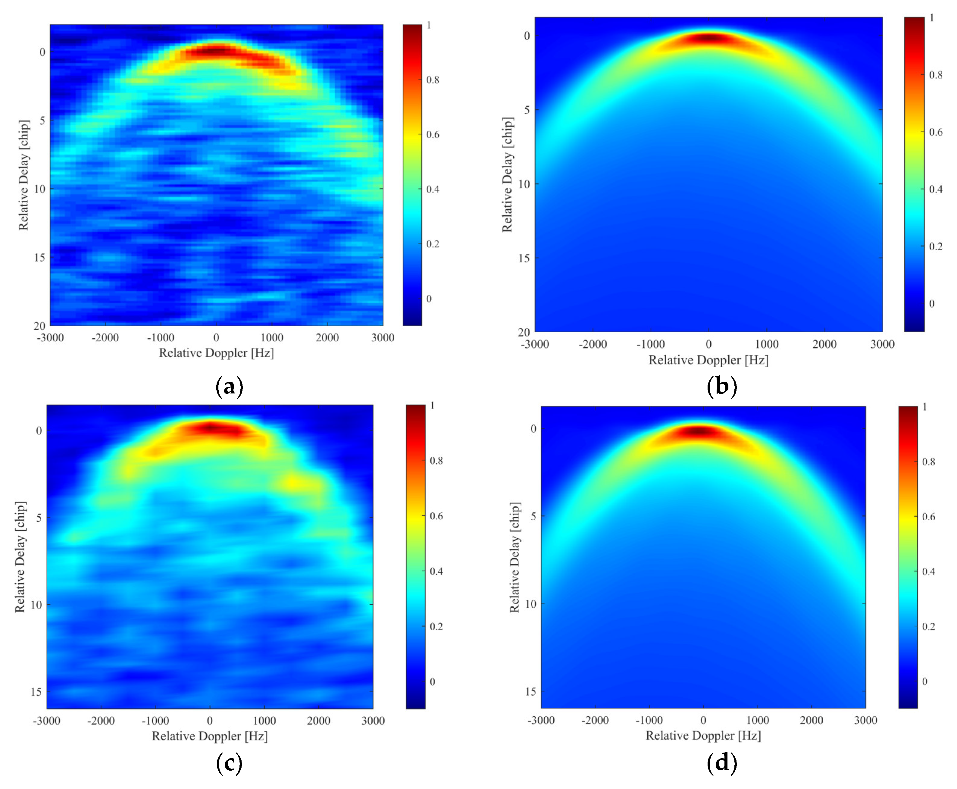
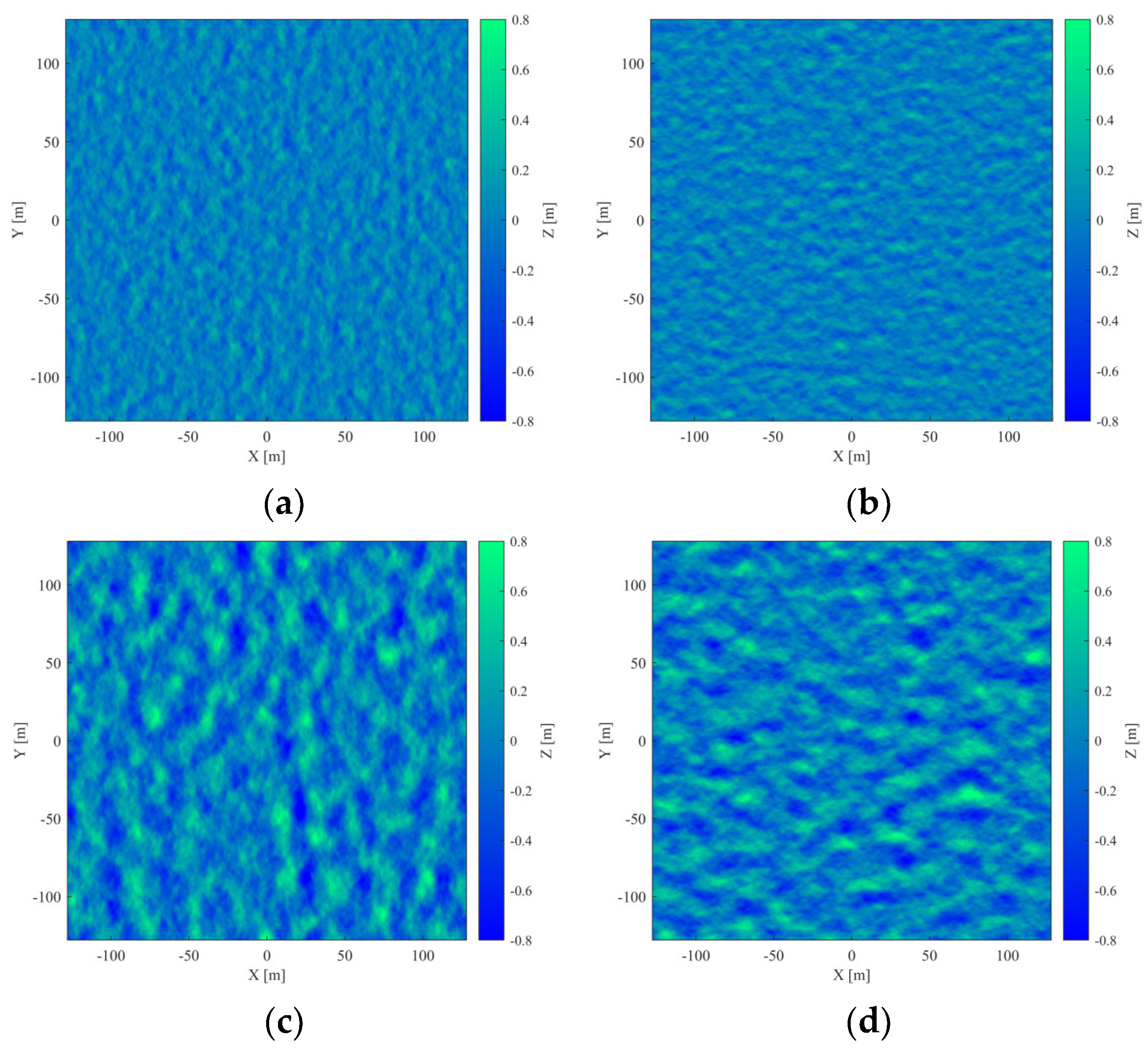
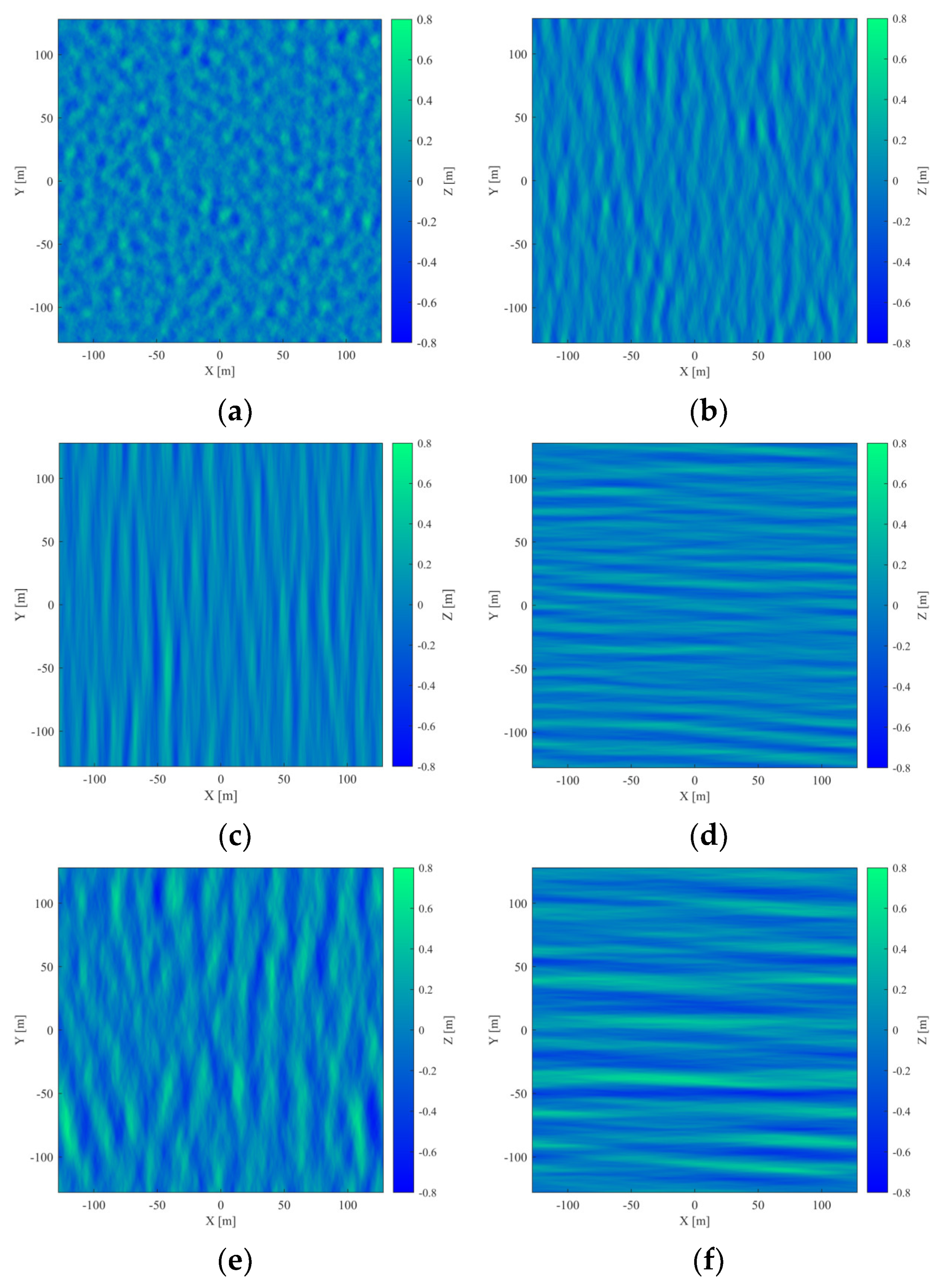
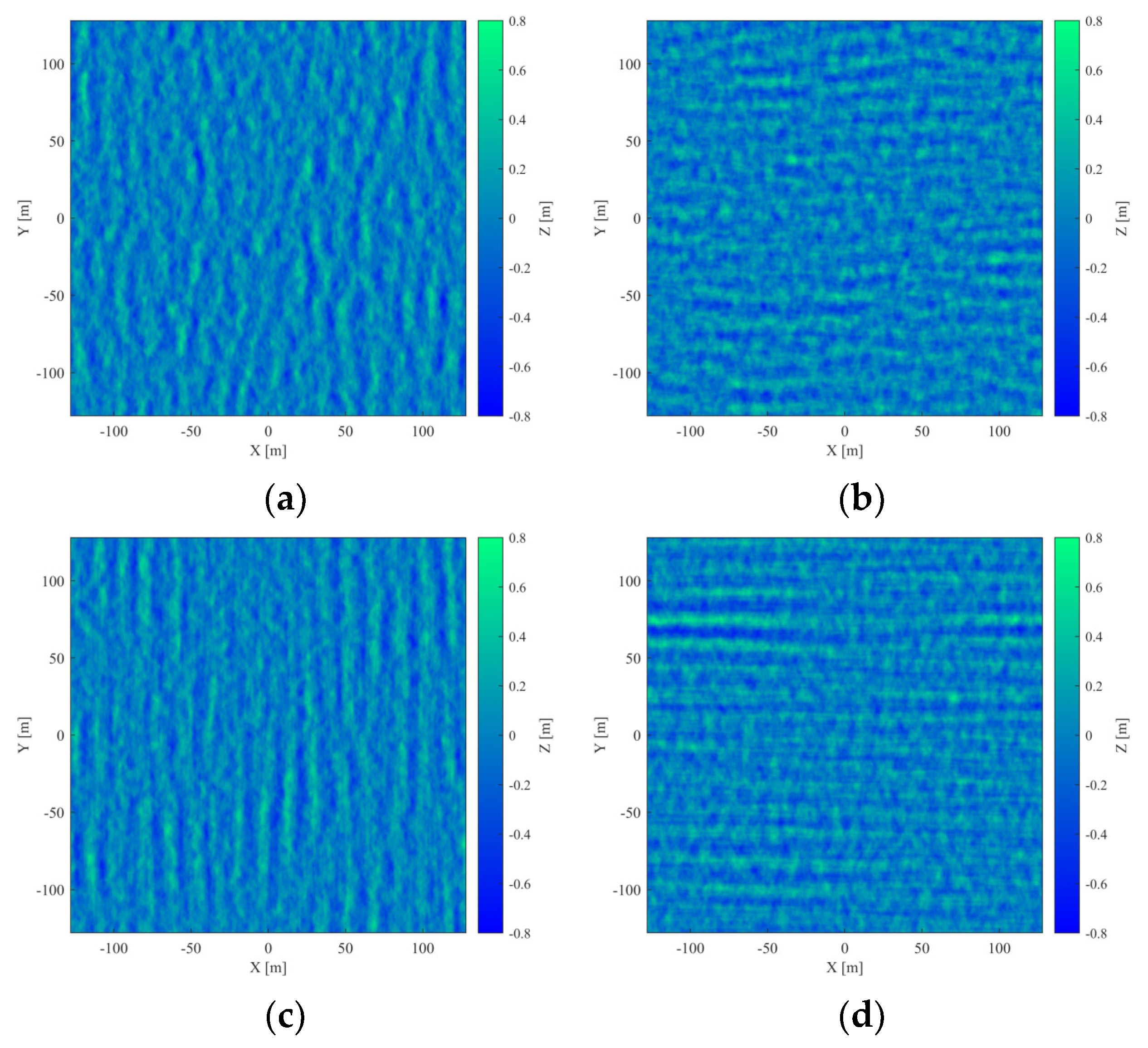
Figure 1. The flowchart of the work in this paper.
Remotesensing 16 01395 g001
Figure 2. The configuration of GNSS bistatic scattering model: the left satellite is the transmitting satellite; the right satellite is the receiving satellite; the black elliptical lines represent the isochronous equal delay rings; the black hyperbola lines represent the equal Doppler lines.
Remotesensing 16 01395 g002
Figure 3. The comparison between the real DDM and simulated DDM. (a) Real UK-DMC DDM [24]; (b) simulated UK-DMC DDM. (c) Real CYGNSS DDM [28]; (d) simulated CYGNSS DDM.
Remotesensing 16 01395 g003
Figure 4. Short-crest wind sea surface simulated by method of filtering Elfouhaily spectrum: (a) wind speed 10 m above sea surface, U10, is 5 m/s, and wind direction ϕw is 0°; (b) U10 is 5 m/s, and ϕw is 90°; (c) U10 is 10 m/s, and ϕw is 0°; (d) U10 is 10 m/s, and ϕw is 90°.
Remotesensing 16 01395 g004
Figure 5. Delay waveforms of different wind speed cases: (a) delay waveforms of unnormalized scattering power, with wind speed ranging from 5 m/s to 20 m/s; (b) delay waveforms of normalized scattering power under the same conditions as (a); and (c) delay waveforms with “dB” procession.
Remotesensing 16 01395 g005
Figure 6. Transformation of simulated wind sea surfaces from short-scale crest to long-scale crest. The size of the sea surface is 256 m × 256 m, and the resolution of each cell is 0.5 m × 0.5 m: (a) U10 is 5 m/s, D is 4, and ϕw is 0°; (b) U10 is 5 m/s, D is 40, and ϕw is 0°; (c) U10 is 5 m/s, D is 400, and ϕw is 0°; (d) U10 is 5 m/s, D is 400, and ϕw is 90°; (e) U10 is 10 m/s, D is 40, and ϕw is 90°; (f) U10 is 10 m/s, D is 400, and ϕw is 90°.
Remotesensing 16 01395 g006
Figure 7. Different MSS results of wind waves under different conditions like U10, D, and ϕw: (a) variation in the MSSx, MSSy, and MSS with U10; (b) variation in the MSS of wind waves with D; (c) variation in the MSS of wind waves with ϕw.
Remotesensing 16 01395 g007
Figure 8. Different types of delay waveforms for various D and U10 cases. (a) Scattering power; (b) normalized scattering power; and (c) normalized scattering power in dB.
Remotesensing 16 01395 g008
Figure 9. Variation in 3-D delay waveforms with different directions and D of wind waves. (a,e) D is 4; (b,f) D is 40; (c,g) D is 400; (d,h) D is 800.
Remotesensing 16 01395 g009
Figure 10. The profile of Figure 9 along the direction of ϕw: (a) near 0 chip and 0.24 chip; (b) near −1.22 chip and 13.43 chip.
Remotesensing 16 01395 g010
Figure 11. Simulations of sea surface with pure 2-D sinusoidal wind wave components under different conditions: (a) wave amplitude A is 1 m, direction of wave ϕw is 0°, and wave length λ is 10 m; (b) A is 1 m, ϕw is 90°, and λ is 10 m; (c) A is 3 m, ϕw is 0°, and λ is 10 m; (d) A is 3 m, ϕw is 90°, and λ is 10 m; (e) A is 3 m, ϕw is 0°, and λ is 50 m; (f) A is 3 m, ϕw is 90°, and λ is 50 m.
Remotesensing 16 01395 g011
Figure 12. Variation in the MSS with amplitude A, wave length λ, and wave direction ϕw. (a) MSS changing with the increase in A; (b) MSS changing with the increase in ϕw.
Remotesensing 16 01395 g012
Figure 13. Variation in 3-D delay waveforms with different directions and D of 2-D sinusoidal long-crest wind waves. (a,c) A = 0.4 m, and D is 400; (b,d) A = 1.0 m, and D is 400.
Remotesensing 16 01395 g013
Figure 14. Simulations of mixed sea surface combining typical short-crest wind waves with 2-D sinusoidal long-crest wind waves under different conditions: (a) wave amplitude A is 1 m, direction of wave ϕw is 0°, and wave length λ is 10 m; (b) A is 1 m, ϕw is 90°, and λ is 10 m; (c) A is 3 m, ϕw is 0°, and λ is 10 m; (d) A is 3 m, ϕw is 90°, and λ is 10 m; (e) A is 3 m, ϕw is 0°, and λ is 50 m; (f) A is 3 m, ϕw is 90°, and λ is 50 m.
Remotesensing 16 01395 g014
Figure 15. Different types of delay waveforms for various wave length λ and amplitude A cases. (a) Scattering power; (b) normalized scattering power; and (c) normalized scattering power in dB.
Remotesensing 16 01395 g015
Figure 16. Variation in 3-D delay waveform in different directions and A of mixed sea surface: (a,e) A = 0.4 m; (b,f) A = 1.0 m; (c,g) A = 2.0 m; (d,h) A = 3.0 m.
Remotesensing 16 01395 g016
Table 1. Parameter configurations of simulated wind sea surface in Figure 6.
Sea Surface SamplesU10ϕwDhe
(a)5 m/s40.7721 m
(b)5 m/s400.7779 m
(c)5 m/s4000.7961 m
(d)5 m/s90°4000.7692 m
(e)10 m/s401.5774 m
(f)10 m/s90°4001.5599 m
Disclaimer/Publisher’s Note: The statements, opinions and data contained in all publications are solely those of the individual author(s) and contributor(s) and not of MDPI and/or the editor(s). MDPI and/or the editor(s) disclaim responsibility for any injury to people or property resulting from any ideas, methods, instructions or products referred to in the content.

