Automated Camera Pose Generation for High-Resolution 3D Reconstruction of Bridges by Unmanned Aerial Vehicles

Abstract

This work explores the possibility of automating the aerial survey of bridges to generate high-resolution images necessary for digital damage inspection. High-quality unmanned aerial vehicle (UAV) based 3D reconstruction of bridges is an important step towards autonomous infrastructure inspection. However, the calculation of optimal camera poses remains challenging due to the complex structure of bridges and is therefore often conducted manually. This process is time-consuming and can lead to quality losses. Research in this field to automate this process is yet sparse and often requires high informative models of the bridge as the base for calculations, which are not given widely. Therefore, this paper proposes an automated camera pose calculation method solely based on an easily accessible polygon mesh of the bridge. For safe operation, point cloud data of the environment are used for automated ground detection and obstacle avoidance including vegetation. First, an initial set of camera poses is generated based on a voxelized mesh created in respect to the quality requirements for 3D reconstruction using defined camera specification. Thereafter, camera poses not fulfilling safety distances are removed and specific camera poses are added to increase local coverage quality. Evaluations of three bridges show that for diverse bridge types, near-complete coverage was achieved. Due to the low computational effort of the voxel approach, the runtime was kept to a minimum, even for large bridges. The subsequent algorithm is able to find alternative camera poses even in areas where the optimal pose could not be placed due to obstacles.

1. Introduction

Bridges constitute an indispensable component of infrastructure, mandating periodic safety assessments. Traditional approaches rely on manual bridge inspections, necessitating a substantial labor force and consequently incurring significant costs. In recent years, research related to the use of unmanned aerial vehicles (UAVs) equipped with cameras has steadily increased. As per the work of Zhang et al. [1], the automated inspection process can be delineated into three phases: data acquisition via camera-equipped UAVs, data processing through automated damage detection software, and bridge condition assessment based on the determined damages. The primary emphasis of these investigations has centered on the second phase, automated damage detection, primarily leveraging deep learning methodologies.

To ensure the optimal performance of the damage detection methods, images captured from the bridge must conform to various quality requirements. These requirements, more detailed and specified later in this work, include considerations related to resolution and the angle of view on the surface, as well as the need for sufficient overlap with adjacent images to facilitate flawless composition into a comprehensive image or 3D model of the bridge. In conventional manual flights, this objective is achieved through the acquisition of an extensive quantity of images, yet this method often leads to unnecessary redundancies, resulting in prolonged computational times for the 3D reconstruction of the bridge, increased on-site time for inspections, and even so, not consistently ensure optimal coverage. Our paper aims to develop a methodology that ensures thorough coverage of the bridge surface through the captured images. First, a method was developed to determine camera poses time efficient even for larger bridges, and therefore, numerous viewpoints. Additionally, an algorithm was developed which adds new camera poses afterwards in insufficiently covered areas to ensure a full coverage of the bridge.

Looking into prior research on viewpoint planning methods for the 3D reconstruction of large-scale objects, in general, a detailed overview is provided by Maboudi et al. [2]. Considering the specific structure of bridges and the necessity of capturing the object from below, a more specialized research field can be delineated. Focusing especially on viewpoint planning for bridges, research is relatively scarce, with only Shang et al. [3] providing a comprehensive overview of previous approaches. In general, three distinct methodologies for viewpoint generation can be delineated, which will be described in the following paragraphs.

In the first method, the sweep-based approach, which is already employed by UAV software providers like Site Scan [4], Pix4D [5], or UgCS [6] for automated surveys, the object is traversed into a grid pattern. Camera poses are positioned based on a bounding box around the object, although they are not further adapted to the object’s geometry, and therefore, keep a high safety distance leading to low image quality. A variation by Peng et al. [7] generates individual planes adjusted roughly to the object’s geometry, resulting in more suitable but not necessarily optimal camera positions.

In the second method, the sampling-based approach, random camera poses are generated and iteratively refined. Bircher et al. [8] divide the object’s surface into small regions, creating a random camera pose for each, subsequently improving to neighboring poses. Shang et al. [9] employ a similar method for generating camera poses but imposes significantly stricter constraints on the allowable space. However, this approach foregoes subsequent optimization of camera poses. In a subsequent paper [3], Shang et al. developed a methodology for post-hoc optimization of camera poses. Another approach by Li et al. [10] places the camera poses by the Poisson disk sampling algorithm and refines the viewpoints in a two-step optimization by minimizing the viewpoint redundancies and maximizing the model point reconstructability.

In the third method, the next-best-view (NBV) approach, camera positions are established within a certain space around the object from which a subset of usable camera poses is computed as an optimization problem. The aim here is to identify the optimal set of poses to best capture the object. Sun et al. [11] select their candidate set based on coverage and overlap parameters, along with flight distance. Schmid et al. [12] also factor in redundancy criteria. In this case, every surface must be viewed from at least two different camera positions from different perspectives. Hoppe et al. [13] employ the same criteria but define conditions for the extent to which camera images must differ to ensure image triangulation. Both Schmid et al. [12] and Hoppe et al. [13] treat the selection of camera poses and route planning as a joint optimization problem. However, they only consider only one flight in their optimization problem, as they focus on a small number of camera poses and not on high-resolution images. While for all NBV approaches the resolution may suffice for 3D reconstruction to capture geometry, it falls short of surveying the structural integrity. A much closer survey requires a significantly higher number of camera poses, rendering optimization infeasible in terms of computational time.

Only Wang et al. [14] present a methodology tailored to close-range aerial surveys of bridges for structural assessment. In this approach, the bridge is divided into its structural components, and camera poses are defined based on predefined patterns for these components. However, this necessitates defining each possible structural component, which may prove challenging given the diversity of bridge structures. Additionally, it presupposes the availability of a building information modeling (BIM) model of the bridge, which may not be accessible in every bridge.

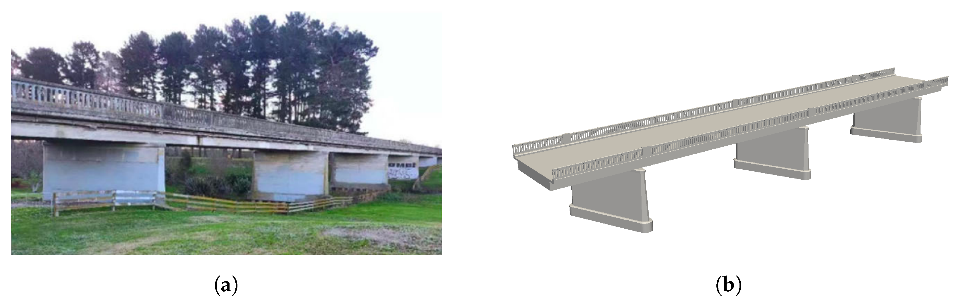
We propose a methodology for the automated generation of camera poses for aerial surface inspection of bridges. We use a surface mesh of the bridge as the data basis for all calculations. Given that bridges are often situated in environments with numerous obstacles such as dense vegetation and other objects, the camera poses are generated with consideration for the surrounding context. Inadmissible camera poses are systematically replaced with others until a comprehensive coverage of the inspectable area is attained through the generated camera poses. All computations are predicated on predefined image quality criteria, UAV and camera specifications, as well as the minimum safety distance pertaining to both the bridge’s surroundings and the bridge itself. Our investigations were conducted on three distinct bridge structures. The results demonstrate that, for all bridges, near-complete coverage of the inspectable areas can be achieved, thereby ensuring the bridge inspection complies with the specified quality standards.

2. Method

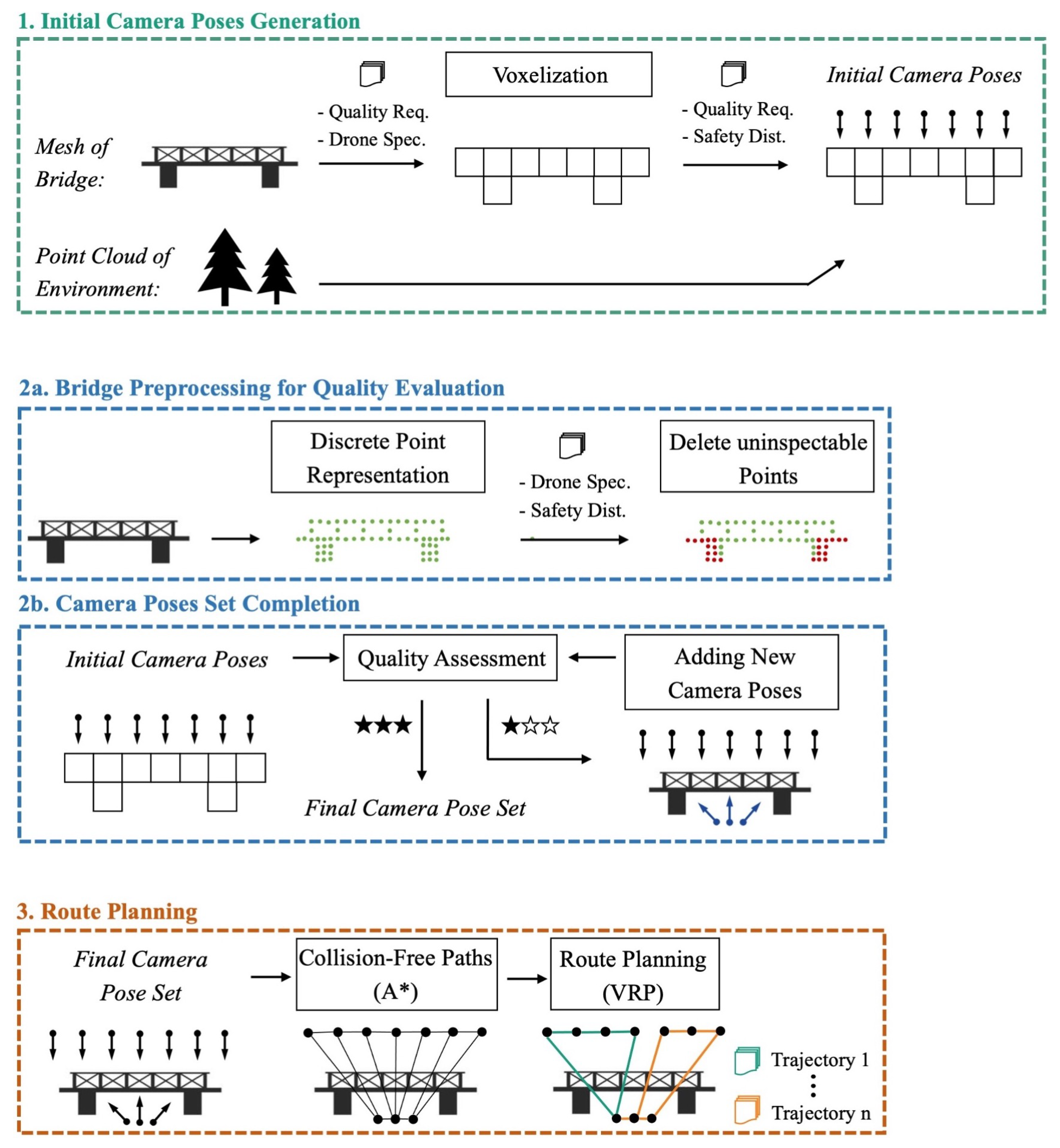
2.1. Method Overview

Figure 1 delineates the procedural framework of the proposed methodology. First, a voxelized representation of the bridge is calculated based on the required quality standards, both in terms of image quality and the overlap factor between individual images. Based thereon, a first set of camera poses is generated, elaborated in Section 2.2.

To set a base for determining the regions of the bridge captured by each camera pose, the surface mesh of the bridge is discretized into points. To speed up later calculations and improve their accuracy, irrelevant points are removed. Subsequently, an evaluation is conducted to identify areas that meet the quality criteria and those requiring the generation of additional camera poses, given the removal of camera poses that fail to adhere to safety distances from the surroundings and the bridge structure. An iterative process is employed to assess coverage quality and add new camera poses until satisfactory coverage quality is achieved. The methodology developed for this purpose is detailed in Section 2.3. Subsequently, the shortest path between individual camera poses is determined using the A* algorithm [15], treating this network as a vehicle routing problem (VRP) to derive optimal flight routes, as discussed in Section 2.4.

2.2. Calculation of Initial Camera Poses

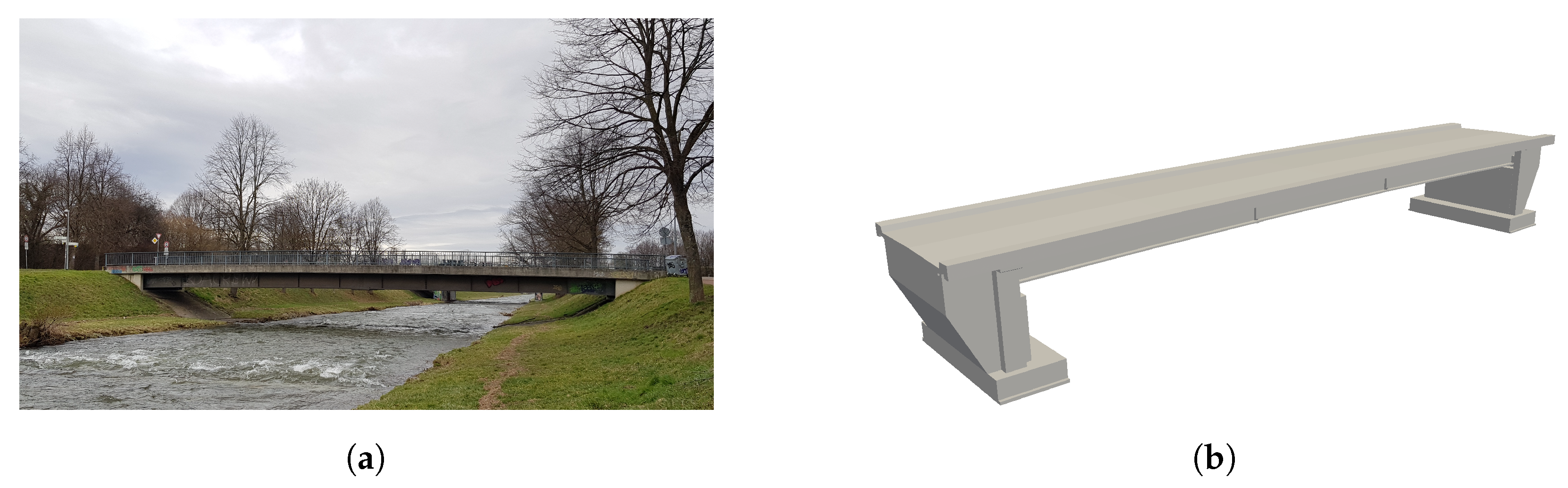
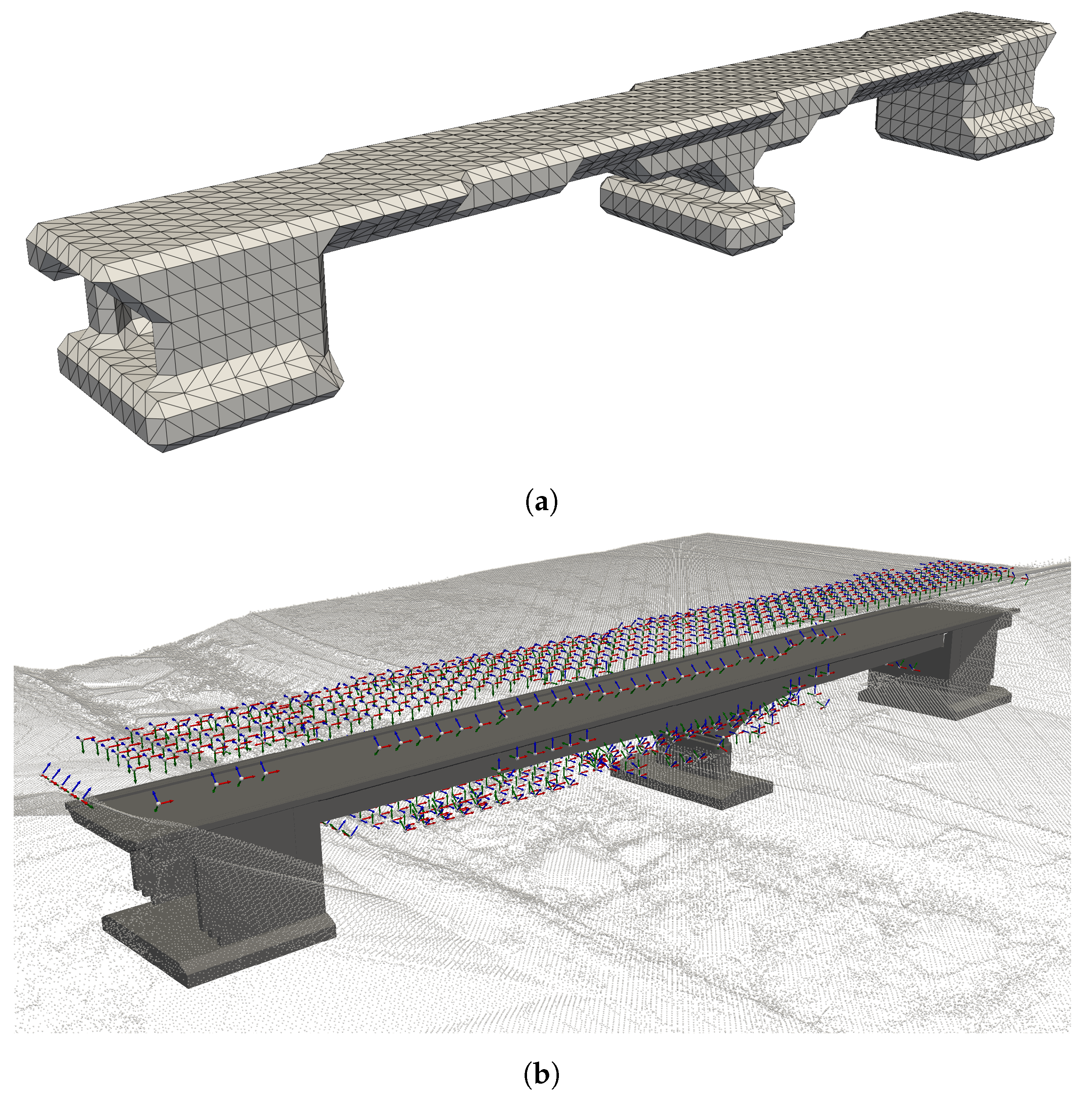
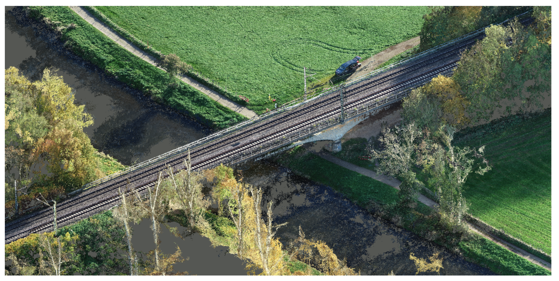
Our fundamental requirement for the computation of camera poses is the availability of a surface mesh representation of the bridge. One approach to acquiring such a mesh involves the utilization of a mesh reconstruction algorithm, such as the Poisson surface reconstruction [16] or Ball-Pivoting [17] Algorithm. Both of these algorithms are applied to a point cloud of the bridge but may yield fragments in the resulting mesh when dealing with noisy or incomplete point clouds. Reconstructing the mesh from satellite imagery is possible but proves impractical due to the absence of information regarding the bridge’s underside. In our methodology, we employ a mesh obtained from bridge construction plans, as detailed by Poku et al. [18], which results in a highly accurate model, even on the underside of the bridge.

The placement of the initial set of camera poses is approached from two distinct perspectives. Firstly, the camera poses should be distributed well along the bridge in regards to the geometrical structure of the bridge in each area to facilitate adequate image overlap and, consequently, successful image reconstruction. However, secondly, the distribution of camera poses should not be over-excessively tailored to the specific geometric characteristics of the bridge, as with a large number of cameras, an unbearable run-time follows. This goal is to adapt the cameras well enough to make the approach applicable to various bridge types while minimizing the algorithm’s computational time. These two objectives, however, inherently compete with each other.

An approach, also employed by Sun et al. [11] in aircraft flyovers, involves representing the object as voxels. This more abstract representation simplifies the object’s geometry while retaining essential information. The size of the voxels is determined based on various parameters, taking into account the image resolution quality requirements and the specifications of the UAV camera. The specific values used are listed in

Table A1. Required parameters, short description, and values used for the algorithm.

Category	Parameter	Description	Value
UAV	Flight speed	UAV’s flight speed between waypoints	3 m/s
	Battery life	-	25 min
Camera	Camera angle	Horizontal and vertical camera field of view	73.89° × 58.90° (5:4)
	Tilt angle	Camera tilt limitations in the lateral axis	−90°, 90°
	Image resolution	-	5344 × 4016 pixels
	Focal length	Actual and 35 mm equivalent	3.92 mm/23 mm
	Sensor width	-	5.9 mm
	Sensor height	-	4.43 mm
Quality	Overlap	Vertical overlap between adjacent images	50%
	Targeted GSD	-	1 mm/pixel
	Saturated distance	Saturation distance between camera and surface	3.02 m
	Saturated incidence angle	Saturation angle between camera and surface	15°
	Maximum incidence angle	Max angle between camera and surface	65°
Safety	Bridge clearance	Minimum clearance from the bridge	2 m
	Environmental clearance	Minimum clearance from the surroundings	2 m

.

From the desired ground sampling distance (GSD), the necessary distance between the UAV and the object can be calculated as

$$\mathrm{distance}\mathrm{between}\mathrm{camera}\mathrm{and}\mathrm{surface}=\frac{\mathrm{GSD}\times \mathrm{Focal}\mathrm{Length}\times \mathrm{Image}\mathrm{Width}}{\mathrm{Sensor}\mathrm{Width}}$$

(1)

with the focal length and sensor width specified in millimeters and the image width given in pixels. The GSD is expressed as millimeters per pixel. The area covered on the bridge can be determined by:

$$\mathrm{Image}{\mathrm{Area}}_{\mathrm{Width}}=\frac{\mathrm{Sensor}\mathrm{Width}\times \mathrm{Distance}}{\mathrm{Focal}\mathrm{Length}}$$

(2)

$$\mathrm{Image}{\mathrm{Area}}_{\mathrm{Height}}=\frac{\mathrm{Sensor}\mathrm{Height}\times \mathrm{Distance}}{\mathrm{Focal}\mathrm{Length}}$$

(3)

The distance, as defined in Equation (1), is expressed in meters. It is important to note that the calculated image area is an approximation, as the equation does not account for uneven surfaces and camera effects such as distortion. To reconstruct a point, images from three perspectives are required [19,20]. This necessitates an overlap of the image areas. Given that in most cameras the image area is typically wider horizontally than vertically, it is prudent to define an overlap factor for the vertical dimension. Ideally, the vertical overlap should also be set to a minimum of 50% to ensure complete 3D reconstruction [21]. The horizontal overlap is determined by the distance between the focal points in the vertical direction. The calculation of the voxel size is illustrated schematically in Figure 2.

The equation for calculating the voxel size results as follows:

$$\mathrm{Voxel}\mathrm{Size}=(1-\mathrm{Overlap}\mathrm{Factor})\times \mathrm{Image}\mathrm{Height}$$

(4)

Placing the camera poses on the voxelized mesh raises the problem that images acquired at the edges of the bridge would be oriented at a 90° angle to each other, resulting in a lack of image overlap and, consequently, making the reconstruction process significantly challenging. To address this issue, we employ the marching cubes algorithm [22] on the voxelized bridge, which changes the object’s edges to a 45° angle relative to each other, facilitating the reconstruction process.

2.3. Creating Additional Camera Poses in Uncovered Areas

The initially placed cameras ideally already cover a significant portion of the bridge with high quality. However, by removing cameras that do not adhere to safety distances, it is unlikely that all inspectable areas are fully captured. Therefore, in the subsequent steps, the initial camera poses are supplemented with additional poses.

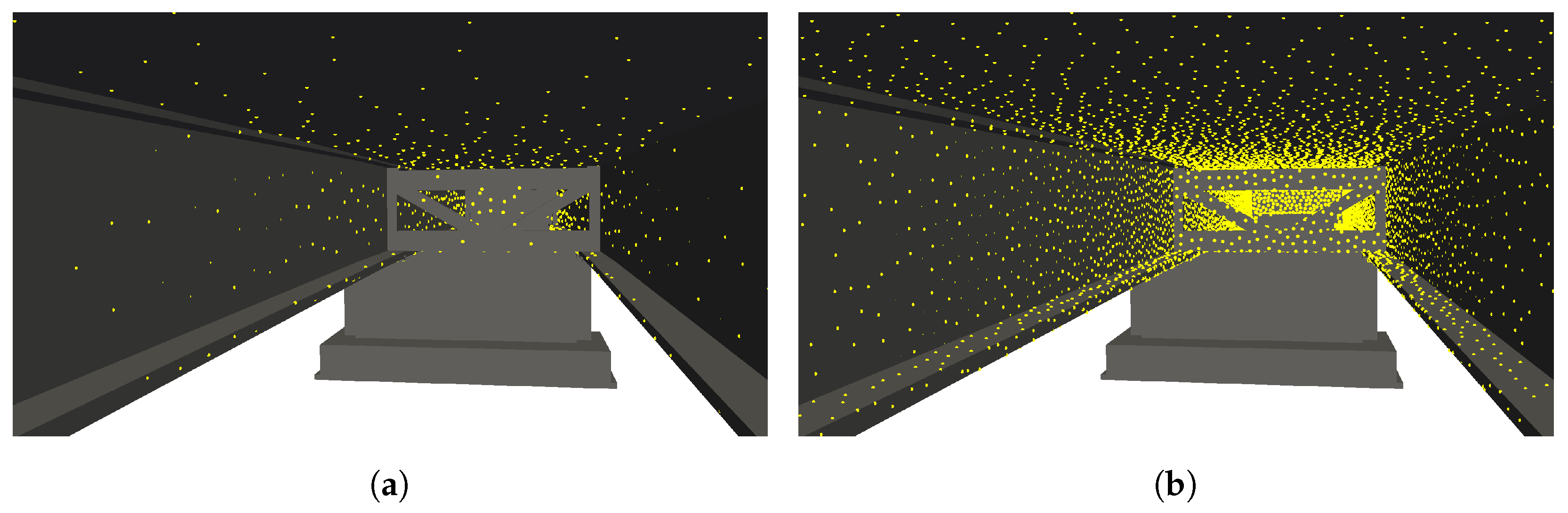
2.3.1. Preprocessing for Quality Evaluation

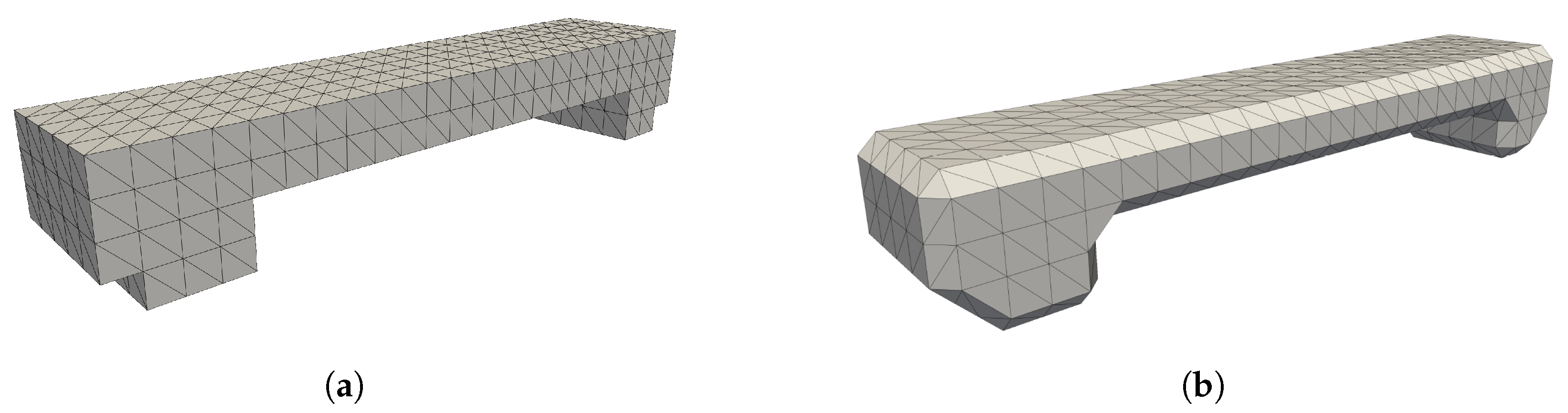
To assess the generated camera poses, evenly distributed points are created over the bridge surface using the Poisson-disk sampling algorithm. These points serve as the basis for evaluating the surface coverage at these locations. In our study, we examined point sets with varying inter-point distances, as depicted in Figure 3. We selected a maximum average distance of 10 cm between the points, as by exceeding this value the points would not adequately represent the object’s geometry. A finer distribution of points is not recommended, as the number of points increases quadratically, resulting in a significant increase in computational time. 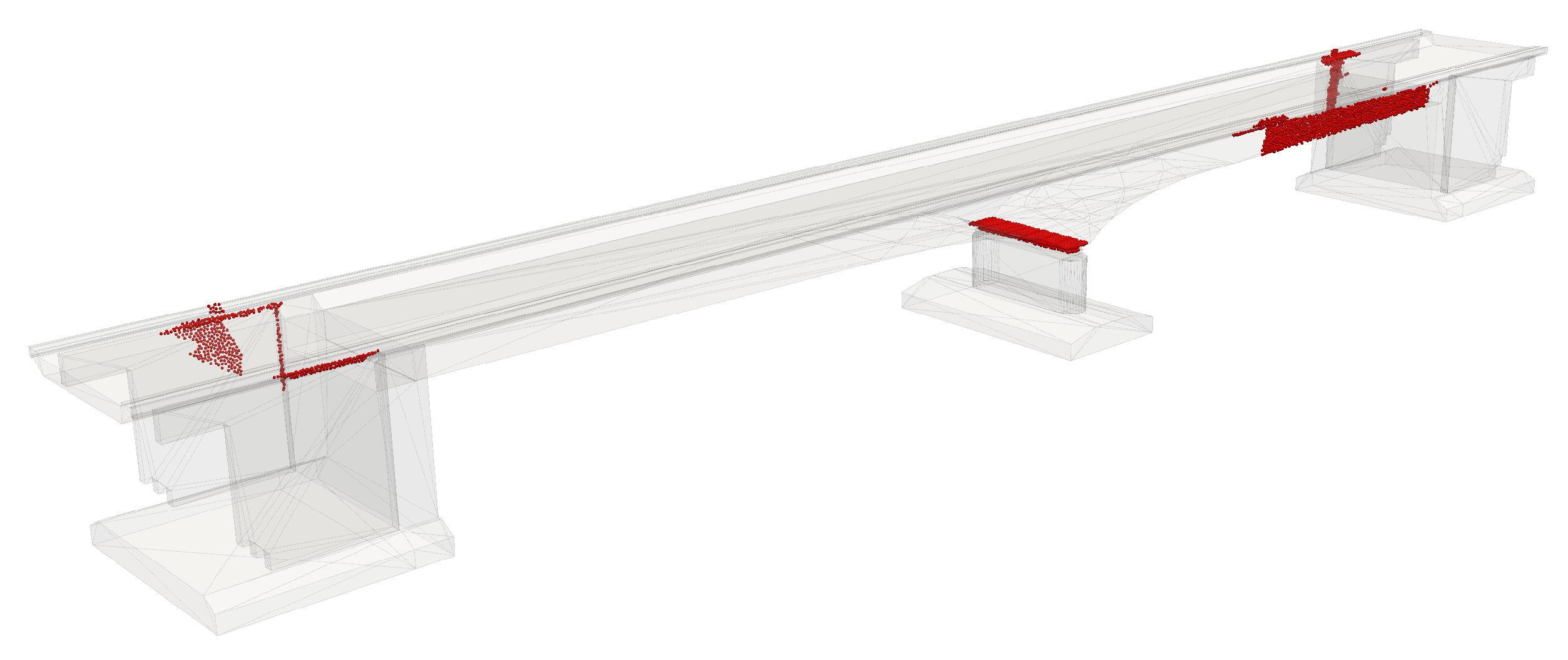The bridge models, such as those from [18], include foundation structures located beneath the ground surface, making them inaccessible for inspection. To obtain more meaningful results and reduce the runtime of the algorithm, non-visible surface points of the bridge are removed.

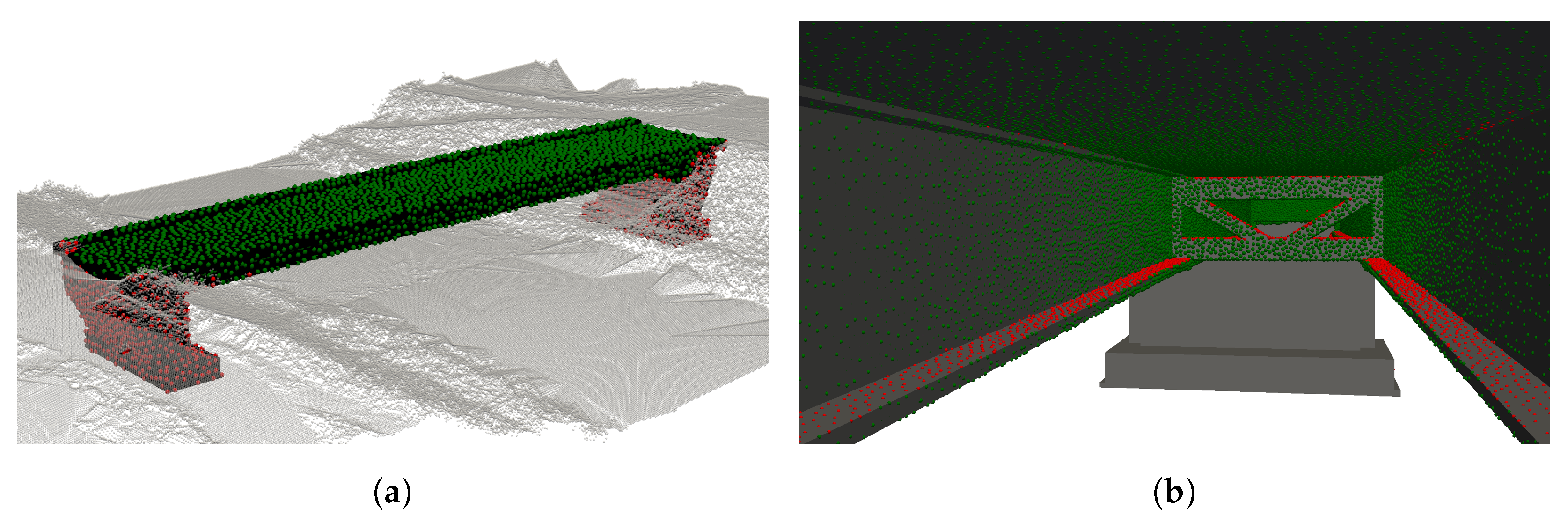
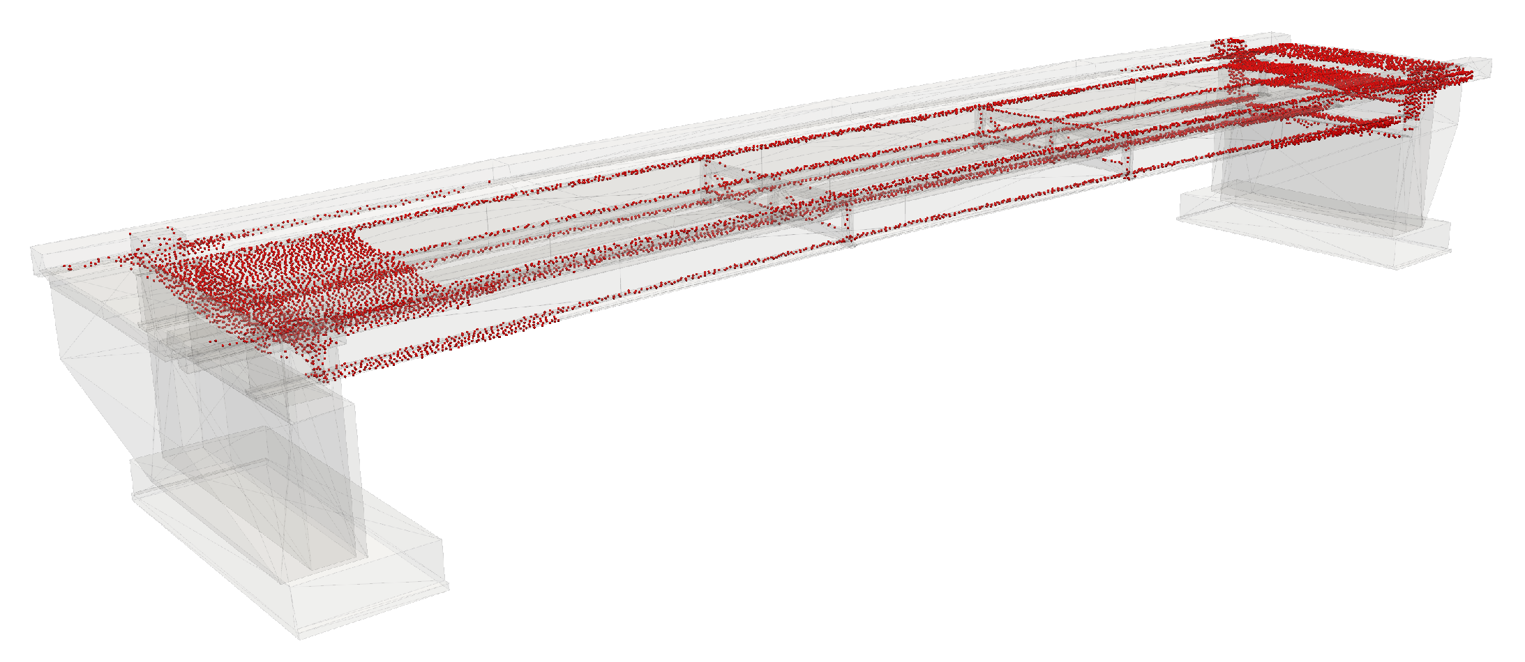
The remaining points are visible through manual inspection, but not necessarily by UAV flights. In some areas of the bridge, it may be impossible to find a feasible camera pose to capture a surface point without violating the necessary safety distances. To prevent the algorithm, described in Section 2.3.3, from attempting to create new camera poses for non-inspectable points, these points are also eliminated from the set of surface points. Inspectable points are determined by densely generating potential camera positions along the perimeter of the no-fly zone. If a surface point is visible from a camera position within the specified maximum incident angle constraints, it is deemed inspectable. Conversely, if no potential camera position can view the point, it is considered non-inspectable. The possible camera positions are generated while accounting for safety distances from the bridge and its surroundings. Figure 4 illustrates both, not visible and not inspectable points.

The final set of points comprises both visible and inspectable points on the bridge surface. This enables more reliable assessments of the algorithm’s coverage percentage while simultaneously reducing run-time through a smaller number of surface points. However, it is important to note that the inspectability of a point does not automatically guarantee its complete reconstruction. Although a point is classified as inspectable if it is visible from at least one camera, a successful reconstruction typically requires images from multiple distinct perspectives. Even so, due to the substantial number of surface points, such an extensive verification process is impractical to implement.

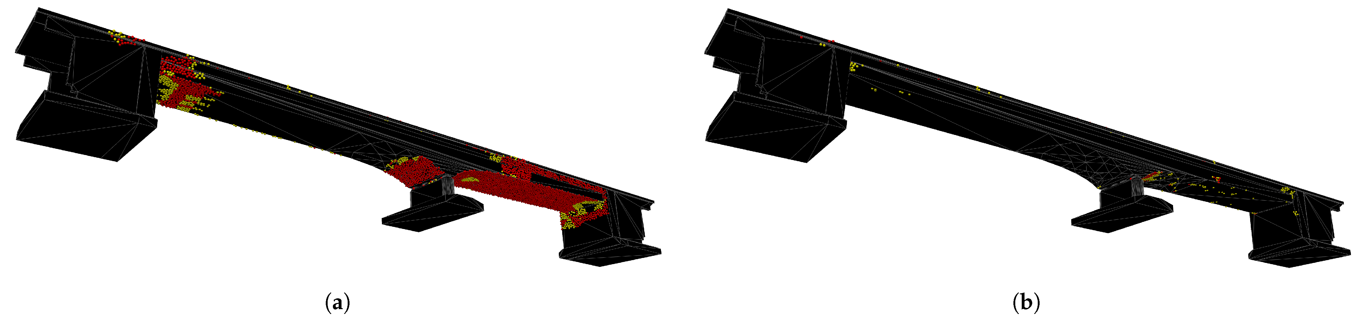
2.3.2. Evaluating Point Reconstruction Quality

The evaluation of the surface points is based on fundamental principles that must be considered for 3D reconstruction [3]:

Principle 1:

Every point on the surface must be captured by at least two [23], and for sparsely textured surfaces, three high-quality images [19,20].

Principle 2:

Small angles between individual images can lead to triangulation errors in depth interpretation [7].

Principle 3:

Redundant images are uninformative and do not increase the reconstruction quality but only the computation time [3].

Based on these fundamental principles, points are categorized. If a point satisfies the first two principles, meaning it is observed from at least three different positions, each with distinct incident angles, the point is considered captured. A point satisfies the first principle, if the points are within the focus range of the drone camera and a maximum angle of 65° between the camera view direction and the surface exists. 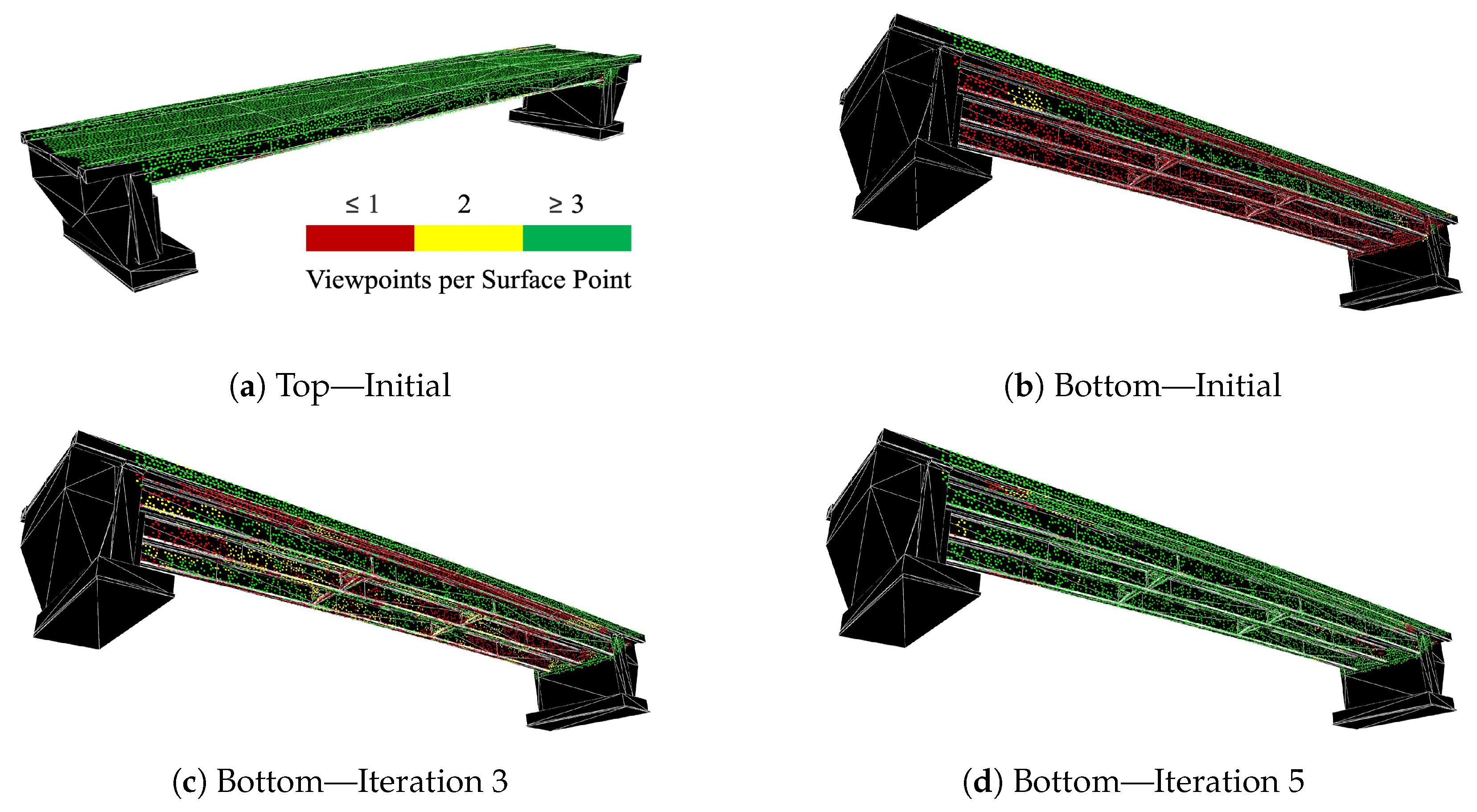For the second principle a minimum angle of 15° has to be between each of the three cameras relative to the others [7]. Once a point is seen by three or more camera poses, each within the quality angle requirements it is not further considered for subsequent calculations, as dictated by principle 3. Consequently, this approach allows for a significant reduction in both the reconstruction run-time and the computational time of the subsequent algorithm for calculating additional camera poses. The calculations are conducted solely based on the points that have not yet been completely captured, leading to a substantial reduction in the run-time without compromising quality.

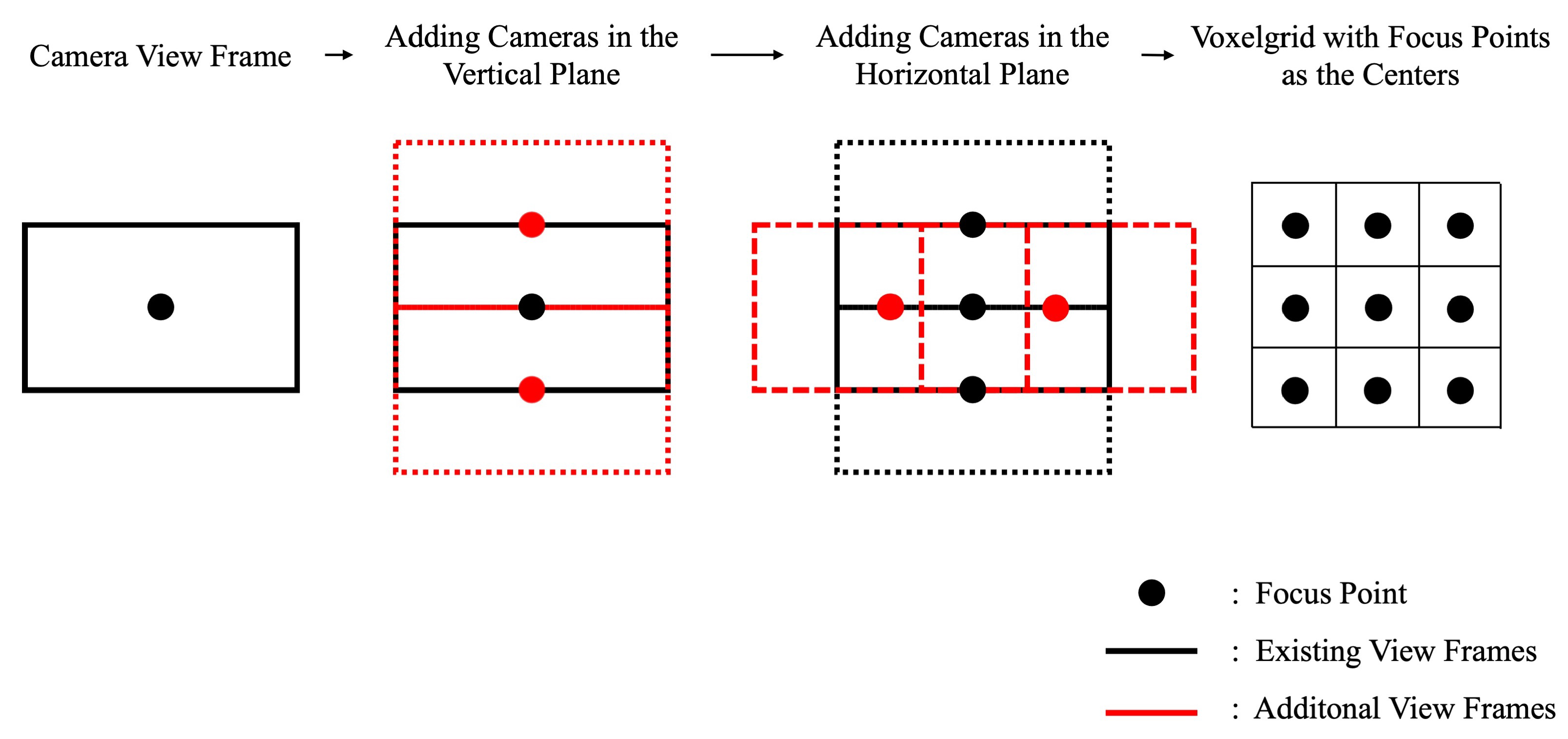
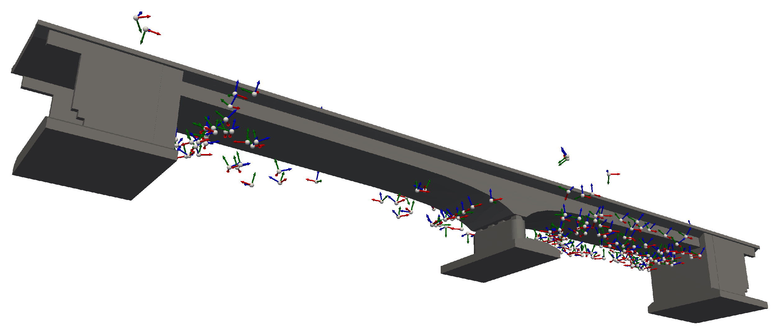
2.3.3. Camera Pose Placement Algorithm

For areas where the coverage of the bridge is not yet complete, new camera poses are generated. The process is divided into three stages: grouping of points, with a new camera pose added for each group. Subsequently, the camera poses are improved in their position and lastly orientation. The process is schematically depicted in Figure 5.

The points are grouped based on voxels, with the bridge area being segmented and points sharing the same voxel clustered together. Empirical tests into the most efficacious voxel sizes were undertaken, culminating in the selection of a voxel size twice that which was employed for the voxels delineated in Section 2.2. A distinct camera pose is generated for each voxel group. The camera poses position is established emanating from the center of the points utilizing the normal vector of the center. The calculated GSD serves as the distance with the camera’s orientation directed towards the central coordinates of the points to ensure focused alignment.

The new camera may be situated in a non-flyable area or may not be optimally placed yet for the group of points. Therefore, variations of the camera position are created, with the camera focus always remaining on the center of the points, and the pose with the highest quality is selected. To avoid creating camera poses that are too similar to existing ones, new poses within close proximity to another pose with a viewing direction deviation of less than 15° are not allowed. The evaluation of the camera quality is based on the assessment of the distance to the points as well as the incident angle. The equation for calculating camera quality is

$$Q(P_{vox},v)=\sum _{p\in P_{vox}}q(p,v),$$

(5)

with $P_{vox}$ representing the set of points in a voxel. The evaluation of the camera-point quality

$$q(p,v)=(1-w)\left(1-\frac{|\mathrm{dist}(p,v)-{\mathrm{dist}}_{\mathrm{sat}}|}{{\mathrm{dist}}_{\max }}\right)+w\left(1-\frac{|\theta (p,v)-{\theta }_{\mathrm{sat}}|}{{\theta }_{\max }}\right)$$

(6)

is derived from Shang et al. [3] and incorporates, in addition to weighting the factors of distance $dist$ and incident angle $\theta$ through parameter w, the normalization and saturation of both factors.

The adjustment in the camera position is limited in relation to the points within the corresponding voxel, preventing the convergence of camera poses towards a singular point with minimal coverage and, consequently, a higher reachable Q score. Instead, the optimization occurs at a local level for each voxel, as visualized in Figure 5a. Following the refinement in position, a global enhancement of the camera poses’ viewing directions takes place, involving all as-yet-uncovered points. This strategic approach, illustrated in Figure 5b, aims to focus the camera poses on localized hotspots. The newly derived camera poses are added to the existing set, prompting a reassessment of points. The iterative repetition of this process continues until comprehensive coverage is achieved for those points that remain incompletely captured.

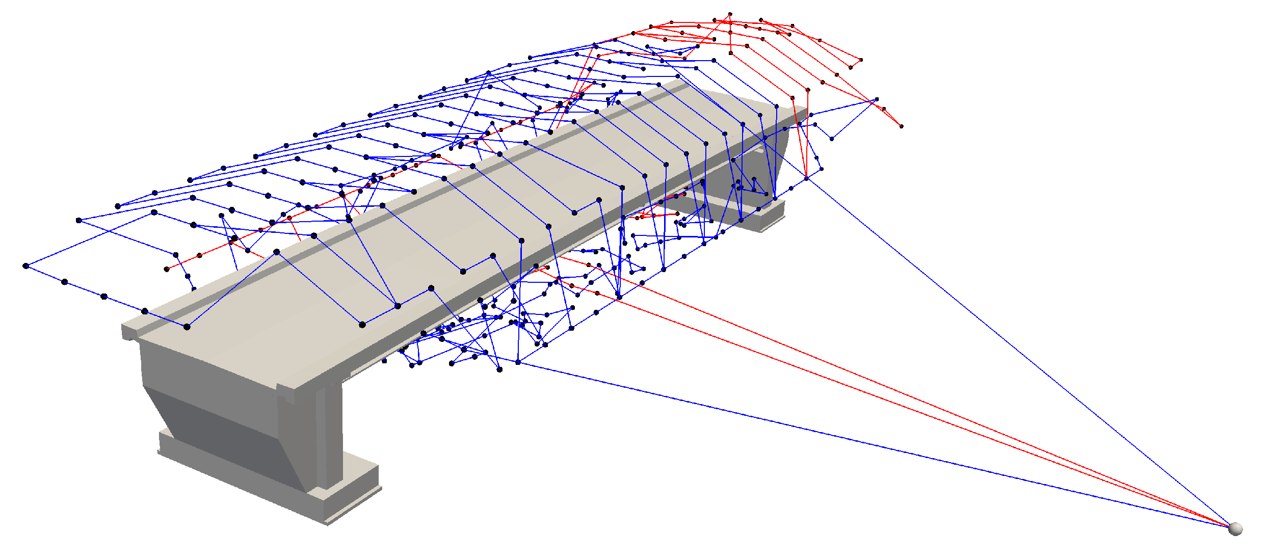
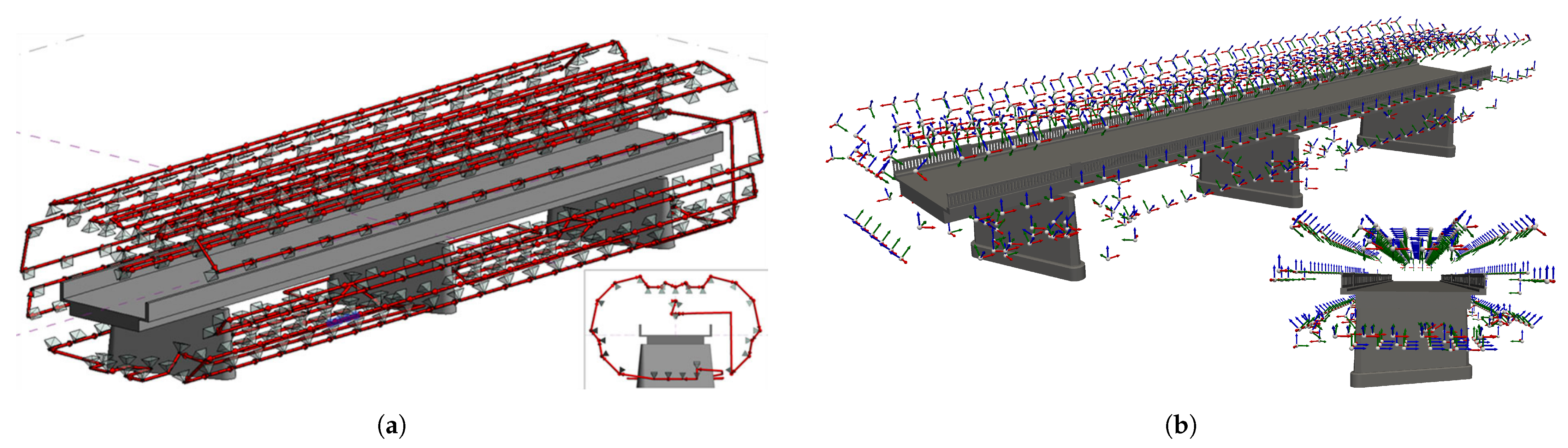
2.4. Path Planning and Route Optimization

The determination of the optimal trajectory, using the calculated camera positions as waypoints, is accomplished through the formulation of a VRP. This formulation places constraints on the flight duration based on the UAV’s battery capacity, for which the following specifications are defined:

Specification 1:

The battery capacity is set to a maximum of 80% of its actual capacity.

Specification 2:

Three seconds are added at each waypoint to account for reduced speed before and after the waypoint, as well as the time required for capturing images.

The connections between waypoints are computed using the A* algorithm. As A* is a graph-based algorithm, the first step involves constructing a network. This is achieved by evenly distributing points on a slightly expanded mesh within the permissible flying area around the bridge, representing the network nodes. The choice of point density has a direct impact on the optimality of the computed route, but it also affects the network’s size and computational time. Edges are established between nodes if the connection between points does not intersect restricted airspace. Additionally, each camera position is connected to all directly accessible network nodes. In the subsequently generated network, the shortest path is computed between each pair of camera poses by the A* algorithm.

The connections between camera positions, determined through A*, form the basis for defining the VRP. Distances between camera positions are converted into flight times. The optimization problem is then solved using the open-source library OR-Tools, developed by Google AI [24].

3. Method Validation

The evaluation has been conducted on three bridges of different sizes and locations. The elaborated methods were implemented in Python, with the methods being tested and evaluated on the bridges virtually. Applying the algorithm in practice poses several challenges, as the GNSS signals for determining the drones position are not sufficient under the bride. Additional positioning methods like Visual Localisation can be used, but remains challenging which will be discussed in future works. The algorithm was evaluated by determining bridge coverage. Surface points along the bridge were categorized as whether they were captured by at least three viewpoints with at least 15° between each viewpoint and a maximum angle of the camera to the surface of 65°. All underlying quality principles were discussed in more detail in Section 2.3.2.

3.1. Bridge 1: Pedestrian Bridge

The first bridge, a pedestrian bridge located in Freiburg, Germany, spanning a river, is depicted in Figure 6 alongside the bridge mesh derived from [18]. In the provided mesh the railings are not included, but as they are not the focus of this investigation they can be accordingly disregarded.

The bridge’s relatively diminutive size posed a challenge for the aerial survey. To achieve a targeted GSD of 1 mm/pixel, the distance of the UAV to the bridge is calculated to be 3.0 m when using the specifications of the UAV Parrot Anafi. However, the bridge’s clearance above the riverbed is just under 2.5 m, rendering it impossible to conduct an aerial survey of the bridge’s underside while adhering to the safety margins of 2.0 m from the surroundings and the bridge, as specified in Table A1. Hence, the study for this bridge maintained a safety margin of 1.5 m from the bridge and 1.0 m from the surroundings, with the understanding that this could only be achieved in a real survey with the use of a UAV safety cage. This assumption, however, allowed for the survey of the underside of the bridge and analysis of the algorithm’s behavior in complex geometries. All calculations were performed with the drone camera specifications of the Parrot Anafi, which allows a camera pitch of 90° in both directions, allowing the drone to capture images from the bridges underside.

With the targeted GSD of 1 mm/pixel, a voxel size of 1.71 m was calculated using Equations (1), (3) and (4). The resulting mesh of the bridge is depicted in Figure 7, alongside the mesh after employing the marching cubes algorithm [22] on the voxelized mesh. By applying the algorithm and thereby smoothing the edges of the bridge representation, additional camera poses are placed along the edges. In Figure 8 the generated camera poses are displayed, with one camera pose per voxel face. Camera poses that do not adhere to the required safety distances from the bridge and its surroundings have been excluded. The environment surrounding the bridge is represented by a sparse point cloud. Large objects, such as trees, were removed from the representation to make the camera poses more easily visible in the image but were still considered in the calculations.

Due to the limited clearance from the ground, the initial cameras were placed solely on the top side of the bridge, which effectively cover the entire top surface of the bridge. However, no poses could be positioned on the underside, necessitating the generation of additional poses in this region. Figure 9 illustrates the corresponding coverage of the bridge. Surface points created as in Section 2.3.1 were colored green when three or more camera poses captured the point within the quality constraints of Section 2.3.2. As displayed, the top surface of the bridge was fully covered by the camera poses, the absence of poses at the underside of the bridge left this area unobserved with the initial cameras. With the placement of these initial cameras, 51.2% of the surface points were captured by three or more cameras, which allows a full 3D reconstruction, using 173 camera poses. The relatively low coverage is a result of the lack of cameras beneath the bridge, as the calculated UAV distance to the object of 1.71 m is within the safety distances to the environment. After applying the algorithm from Section 2.3.3, new camera poses were placed to improve the coverage of the bridge. Figure 9 displays the process of the algorithm over the course of five iterations. The newly placed camera poses increased the coverage of the inspectable surface to 94.9% after three iterations and finally 96.7% after five iterations with in total 456 camera poses created. Detailed results of all iteration steps are given in

Table 1. Results of iteration steps for the pedestrian bridge in Freiburg. Algorithm stopped after five iterations as no notable improvement was achieved afterwards.

Iteration	Camera Poses	Percentage Coverage with		Total Runtime
		2 Camera Poses	3 Camera Poses
0	173	51.2%	49.8%	5 min
1	243	80.3%	66.0%	11 min
2	306	92.0%	82.9%	22 min
3	364	94.9%	88.8%	38 min
4	411	96.1%	91.1%	61 min
5	456	96.7%	92.1%	73 min
6	489	97.1%	92.9%	76 min
…	…	…	…	…
10	542	98.3%	94.1%	131 min

.

The inability to achieve 100% coverage after more than ten iterations is attributed to the fact that some inspectable points cannot be captured from multiple distinct viewpoints. As described in Section 2.3.1, points are considered inspectable if they can be observed from at least one camera position, but for reconstruction, at least two images from different perspectives are required. Since the incremental gain in coverage diminishes significantly with each iteration, while the number of added cameras increases disproportionately at a certain point, it is advisable to terminate the algorithm at an appropriate juncture. For this bridge, the computed viewpoint set after five iterations was chosen as the final set, as the improvement in the covered area in subsequent iterations was less than one percentage point.

The 4% of the surface that remained unobserved by the algorithm and the points marked as uninspectable in advance, constituting 15% of the total surface, amount to a total of 18.4% of uninspected surface. The depiction of all uninspected points is presented in Figure 10 which serves as a schematic representation of areas yet to be examined. This provides the opportunity to selectively inspect only these areas in a manual examination, resulting in significantly greater time efficiency. The final algorithm results are summarized in

Table 2. Final results for the investigation of the pedestrian bridge. Coverage of camera poses calculated on the inspectable surface points, hence the final inspected surface is the product of those two values.

Parameter	Value
Runtime	73 min
Iteration steps	5
Required camera poses	456
Coverage by at least two camera poses	96.7%
Coverage by at least three camera poses	92.1%
Inspectable surface	85.2%
Final inspected surface	81.6%
Average GSD	0.99 mm/pixel

. In total 92.1% of the total surface can be captured from 456 viewpoints, with an average GSD of 0.99 mm/pixel.

The runtime of the algorithm for five iterations is 73 min, this is relatively high and is the result of two circumstances. First, the computational cheap initial cameras did not cover nearly half of the bridge surface, therefore, many camera poses had to be created in each run of the algorithm. Furthermore, calculating those poses was time-consuming, as the allowed space under the bridge is small, and therefore, finding an allowed yet suitable pose was difficult.

Route Planning

The calculated points are intended to be traversed with a trajectory of utmost efficiency, wherein the camera positions are regarded as a VRP. The Euclidean distance between two camera positions defines the cost associated with connecting the two nodes. In cases where the direct connection is obstructed by the bridge or its surroundings, A* is employed for path planning. The closer the cameras are positioned to the bridge, the fewer pairs of cameras possess a direct connection; consequently, A* must be applied more frequently. The computational time required for the connections using A* increases disproportionately with the size of the bridge. Examining the routes computed as VRP reveals that none of the trajectories calculated by A* are part of the final solution. The computed distances are so expensive that they are not suitable for the optimal route. A more optimal approach involves linking nearby waypoints without the need for A*. For a network from which the connections computed by A* were removed, similar route results could be achieved. Accordingly, it is sensible to reduce the computational time by initially performing route calculation without A* and only resorting to it when a route cannot be found.

The distances between camera positions were converted into flight times, assuming a flight speed of 4 m/s and incorporating a dwell time of three seconds for the UAV to decelerate, position the camera, and accelerate again at each camera point. A starting and ending point for the UAV was selected as a location 30 m away and 10 m above the bridge. The calculated routes are presented in Figure 11 with the route data provided in

Table 3. Computed routes for the pedestrian bridge.

Parameter	Values
Number of routes	2
Total flight time	26.5 min
Individual routes	Route 1: 20 min
	Route 2: 6.5 min

, both for the pedestrian bridge. Upon examination of the routes, it becomes evident that they are collision-free and that all points are completely traversed, although some routes are not optimal, necessitating a higher run-time of the solver if desired.

3.2. Bridge 2: Railway Bridge

The second examined bridge was a railway bridge in Aachen, depicted as a point cloud with its surroundings in Figure 12. With a length of approximately 120 m, it is the largest bridge investigated in this study. Preceding the analysis, certain areas at both ends of the bridge and at the central support were deemed non-inspectable due to obstacles in the vicinity. These areas are illustrated in Figure 13, constituting 10.2% of the visible surface. For the investigation, as specified in Table A1, a safety distance of two meters was maintained both from the bridge and its surroundings.

The bridge is slightly tilted within the voxel grid, resulting in discontinuities in the voxelized model at certain locations along the bridge, as depicted in Figure 14a. While aligning the bridge within the voxel grid would be feasible for this particular bridge, it may not be achievable for every bridge. Curved bridges, for instance, inherently possess these discontinuities. Consequently, a few cameras in Figure 14b are not optimally aligned at these discontinuities.

The coverage of the bridge by voxel-based cameras is 77.3%, with a minimum of three camera poses per point. Over the course of three iterations, this value could be increased to 95.1% coverage. Due to the already high percentage capture of voxel-based camera poses, the algorithm’s runtime was only 31 min, despite the bridge’s substantial size. The values for each iteration step are listed in

Table 4. Results of iteration steps for the railway bridge. Algorithm stopped after three iterations as no notable improvement was achieved afterwards.

Iteration	Camera Poses	Percentage Coverage by		Total Runtime
		2 Camera Poses	3 Camera Poses
0	764	80.2%	77.3%	7 min
1	857	91.0%	83.3%	12 min
2	909	97.7%	91.5%	25 min
3	944	98.2%	95.1%	31 min
4	979	98.8%	96.1%	39 min
5	998	99.0%	96.5%	43 min
…	…	…	…	…
10	1065	99.7%	98.2%	84 min

, and the final algorithm values after three iterations are summarized in

Table 5. Final results for the investigation of the railway bridge.

Parameter	Value
Runtime	31 min
Iteration steps	3
Required camera poses	944
Coverage by at least two camera poses	98.2%
Coverage by at least three camera poses	95.1%
Inspectable surface	89.8%
Final inspected surface	88.2%
Average GSD	1.07 mm/pixel

. With 944 camera poses, 88.2% of the bridge, which spans over 120 m, was captured with an average GSD of 1.07 mm/pixel. Figure 15 illustrates the areas not covered by the initial and final camera pose sets, Figure 16 displays the poses added in the three iterations. The added poses were positioned predominantly on the underside of the bridge, as anticipated. While the pose placement may initially appear random, closer examination reveals that the cameras mostly maintain a consistent distance from the bridge. The positioning was carried out on a plane where the distance is sufficiently large to capture all points of the respective voxel group and simultaneously small enough to meet the requirement of high image quality.

3.3. Bridge 3: Highway Bridge

Regarding the topic of this work, the aerial survey of bridges for high-resolution image generation, only one paper with a similar thematic stance has been published thus far. To contextualize the findings of this work within the current state of the art, the bridge model used by Wang et al. [14] has graciously been made available. The bridge, located in Hastings, New Zealand is illustrated in Figure 17.

As evident from Figure 17b, the surroundings of the bridge are sparsely vegetated, posing no challenges for the placement of voxel-based camera poses. Only a few points at the end of the bridge, where the surface inclines, are not inspectable by the UAV. Accordingly, with the initial set of poses, nearly 88% of the bridge has already been fully captured. Similar to Wang et al., the underside of the bridge was not inspected to establish a comparable basis. However, the bridge piers remain part of the investigation.

In Figure 18, the camera poses computed by Wang et al. and those derived through our methodology are depicted. Results from both approaches are listed in

Table 6. Comparison of the results between our approach, Wang et al., and an implementation of a Sweep-based approach [25].

Parameter	Our Approach	Wang et al. [14]	Sweep-Based
Required camera poses (initial/final)	619/662	571	755
Avg. GSD (mm/pixel)	1.14	1.51	2.43
Runtime	38 min	-	-
Coverage with two camera poses	99.6%	-	-
Coverage with three camera poses	98.1%	-	-

, along with a method conducted by Wang et al. derived from the current practice in flight plan generation for photogrammetric reconstruction [25]. In all three approaches, the camera specifications of the UAV DJI Phantom 4 Pro v2.0 and an image overlap factor of 66.7% were employed. For our investigation, as with the other bridges previously considered, a GSD of 1 mm/pixel was targeted to ensure automated crack detection on high-resolution images. Wang et al., on the other hand, utilized a GSD of 1.5 mm/pixel.

In our investigation, the voxel-based approach already covered 88% of the inspectable surface, with the non-covered areas primarily located around the bridge piers. The addition of extra camera poses increased the overall coverage to 98.1%. The number of required cameras is 16% higher than that employed by Wang et al., a difference that can be attributed to two main factors. Firstly, our study utilizes a higher GSD, resulting in an increased camera count. Secondly, the placement of cameras based on a BIM model, as employed by Wang et al., is significantly more adapted and, therefore, more efficient than our voxel-based placement. Consequently, camera pose placement based on a BIM model is preferable to the voxel-based method, under the conditions that firstly, a BIM model of the bridge is available, which may not be the case, particularly for smaller or older bridges. And secondly, all structural components used in the bridge have been predefined, as is necessary in Wang et al.’s approach. The use of voxels represents a good, if not equally efficient, alternative when no BIM model of the bridge is available. However, the methodology for placing additional camera poses in areas not yet fully covered presents a compelling opportunity to enhance coverage retrospectively for both voxel and BIM-based approaches. Compared to Wang et al.’s implementation of [25], our approach is significantly superior in both the number of poses used and the average achieved GSD.

4. Conclusions

This paper explores the possibility of automating the UAV camera pose generation for bridges to generate high-resolution images necessary for digital damage inspection and 3D reconstruction to overcome time and labor-consuming manual inspection.

Camera poses are generated based on a voxelized mesh with the size of the voxels calculated from quality requirements and camera specifications with poses being checked for their safety distances to the bridge and the surroundings where disallowed camera poses are removed. The hereby unscanned areas were approached by a second algorithm with inadequately covered areas being grouped and new camera poses then being created and optimized in their position and orientation to the uncovered points. The process was iteratively repeated until complete coverage of the bridge was achieved.

The methodology was applied to three different bridges with varying structural components to validate the general applicability of the developed approach. Almost complete coverage was achieved for all three bridges. The voxel-based approach offers a significant advantage, especially for large bridges, as the majority of the bridge can be covered computationally efficiently with camera poses still tailored well to the geometry of the bridge in each area. The placement of additional cameras in incompletely covered areas is computationally intensive, and therefore, sensible only as a complement to voxel-based placement. However, applying this algorithm significantly increases the coverage for all three bridges, achieving almost maximum coverage of inspectable points. Complete coverage is practically impossible, as each point must be captured from three different positions, which is not achievable for every point.

Overall, this paper, through the combination of a computationally efficient, voxel-based method and individual placement of additional cameras in uncovered areas, provides the opportunity to calculate optimal camera poses for high-resolution 3D reconstruction and damage detection, even for large bridges. The inclusion of the bridge environment elevates the study to a practically applicable level, especially since many bridges are located in densely vegetated surroundings.

A potential improvement for this approach in future work lies in the improvement of the first voxel-based camera pose placement. In this study, poses based on voxels were not further optimized. However, for curved bridges, discontinuities arise along the voxelized mesh, causing sub-optimal orientation of camera poses to the bridge. A post-adjustment may here be beneficial. If a BIM-model of the bridge is available, a combination of our approach with Wang et al. [14] could be of interest, where, instead of the voxel-based approach, cameras are placed according to Wang et al., and for areas where camera poses were not placed due to safety distances, additional cameras could be generated using our second algorithm.

References

1. Zhang, C.; Zou, Y.; Wang, F.; del Rey Castillo, E.; Dimyadi, J.; Chen, L. Towards fully automated unmanned aerial vehicle-enabled bridge inspection: Where are we at? Constr. Build. Mater. 2022, 347, 128543. [Google Scholar] [CrossRef]
2. Maboudi, M.; Homaei, M.; Song, S.; Malihi, S.; Saadatseresht, M.; Gerke, M. A Review on Viewpoints and Path Planning for UAV-Based 3-D Reconstruction. IEEE J. Sel. Top. Appl. Earth Obs. Remote Sens. 2023, 16, 5026–5048. [Google Scholar] [CrossRef]
3. Shang, Z.; Shen, Z. Flight Planning for Survey-Grade 3D Reconstruction of Truss Bridges. Remote Sens. 2022, 14, 3200. [Google Scholar] [CrossRef]
4. Drohnenbasierte Kartenerstellung und Bildanalyse in der Cloud|Site Scan for ArcGIS. Available online: https://www.esri.com/de-de/arcgis/products/site-scan-for-arcgis/overview (accessed on 15 January 2024).
5. Professional Photogrammetry and Drone Mapping Software|Pix4D. Available online: https://www.pix4d.com/ (accessed on 15 January 2024).
6. Ground Station Software|UgCS PC Mission Planning. Available online: https://www.ugcs.com/ (accessed on 15 January 2024).
7. Peng, C.; Isler, V. Adaptive View Planning for Aerial 3D Reconstruction. Proc.-IEEE Int. Conf. Robot. Autom. 2018, 2019, 2981–2987. [Google Scholar] [CrossRef]
8. Bircher, A.; Alexis, K.; Burri, M.; Oettershagen, P.; Omari, S.; Mantel, T.; Siegwart, R. Structural inspection path planning via iterative viewpoint resampling with application to aerial robotics. Proc.-IEEE Int. Conf. Robot. Autom. 2015, 2015, 6423–6430. [Google Scholar] [CrossRef]
9. Shang, Z.; Bradley, J.; Shen, Z. A co-optimal coverage path planning method for aerial scanning of complex structures. Expert Syst. Appl. 2020, 158, 113535. [Google Scholar] [CrossRef]
10. Li, Q.; Huang, H.; Yu, W.; Jiang, S. Optimized Views Photogrammetry: Precision Analysis and a Large-Scale Case Study in Qingdao. IEEE J. Sel. Top. Appl. Earth Obs. Remote Sens. 2023, 16, 1144–1159. [Google Scholar] [CrossRef]
11. Sun, Y.; Ma, O. Automating Aircraft Scanning for Inspection or 3D Model Creation with a UAV and Optimal Path Planning. Drones 2022, 6, 87. [Google Scholar] [CrossRef]
12. Schmid, K.; Hirschmüller, H.; Dömel, A.; Grixa, I.; Suppa, M.; Hirzinger, G. View planning for multi-view stereo 3D Reconstruction using an autonomous multicopter. J. Intell. Robot. Syst. Theory Appl. 2012, 65, 309–323. [Google Scholar] [CrossRef]
13. Hoppe, C.; Wendel, A.; Zollmann, S.; Pirker, K.; Irschara, A.; Bischof, H.; Kluckner, S. Photogrammetric Camera Network Design for Micro Aerial Vehicles. In Proceedings of the Computer Vision Winter Workshop, Mala Nedelja, Slovenia, 1 February 2012. [Google Scholar]
14. Wang, F.; Zou, Y.; del Rey Castillo, E.; Ding, Y.; Xu, Z.; Zhao, H.; Lim, J.B. Automated UAV path-planning for high-quality photogrammetric 3D bridge reconstruction. Struct. Infrastruct. Eng. 2022, 1–20. [Google Scholar] [CrossRef]
15. Hart, P.E.; Nilsson, N.J.; Raphael, B. A Formal Basis for the Heuristic Determination of Minimum Cost Paths. IEEE Trans. Syst. Sci. Cybern. 1968, 4, 100–107. [Google Scholar] [CrossRef]
16. Kazhdan, M.; Bolitho, M.; Hoppe, H. Poisson Surface Reconstruction. In Proceedings of the Eurographics Symposium on Geometry Processing, Cagliari, Italy, 26–28 June 2006. [Google Scholar]
17. Bernardini, F.; Mittleman, J.; Rushmeier, H.; Silva, C.; Taubin, G. The ball-pivoting algorithm for surface reconstruction. IEEE Trans. Vis. Comput. Graph. 1999, 5, 349–359. [Google Scholar] [CrossRef]
18. Poku-Agyemang, K.N.; Reiterer, A. 3D Reconstruction from 2D Plans Exemplified by Bridge Structures. Remote Sens. 2023, 15, 677. [Google Scholar] [CrossRef]
19. Luong, Q.T.; Faugeras, O.D. The fundamental matrix: Theory, algorithms, and stability analysis. Int. J. Comput. Vis. 1996, 17, 43–75. [Google Scholar] [CrossRef]
20. Rumpler, M.; Irschara, A.; Bischof, H. Multi-View Stereo: Redundancy Benefits for 3D Reconstruction. In Proceedings of the 35th Workshop of the Austrian Association for Pattern Recognition, Graz, Austria, 26–27 May 2011. [Google Scholar]
21. Liu, Y.F.; Nie, X.; Fan, J.S.; Liu, X.G. Image-based crack assessment of bridge piers using unmanned aerial vehicles and three-dimensional scene reconstruction. Comput.-Aided Civ. Infrastruct. Eng. 2020, 35, 511–529. [Google Scholar] [CrossRef]
22. Lorensen, W.E.; Cline, H.E. Marching cubes: A high resolution 3D surface construction algorithm. Comput. Graph. 1987, 21, 7–12. [Google Scholar] [CrossRef]
23. Hartley, R.; Zisserman, A. Multiple View Geometry in Computer Vision; Cambridge University Press: Cambridge, UK, 2004. [Google Scholar] [CrossRef]
24. OR-Tools|Google Developers. Available online: https://developers.google.com/optimization/ (accessed on 15 January 2024).
25. Chen, S.; Laefer, D.F.; Mangina, E.; Zolanvari, S.I.; Byrne, J. UAV bridge inspection through evaluated 3D reconstructions. J. Bridge Eng. 2019, 24, 05019001. [Google Scholar] [CrossRef]
Figure 1. Schematic overview of the entire process. In step 1, cameras are computed based on a voxelized representation of the bridge, and cameras with insufficient safety margins are removed. In step 2, the bridge is represented as a point cloud, allowing for the evaluation of the quality of the previous capture. Where necessary, additional cameras are generated iteratively. Finally, in step 3, trajectories along the camera positions are calculated.
Remotesensing 16 01393 g001
Figure 2. Methodical approach for calculating the voxel size. Camera view frames are vertically positioned with the required overlap, and horizontally placed at equal intervals. The camera focal points are set at the voxel center.
Remotesensing 16 01393 g002
Figure 3. Discrete surface representation via the Poisson-Disk sampling algorithm. In (a), a mean distance of 0.3 m between points was chosen, yet the bridge structure is not accurately represented. In (b), a mean distance of 0.1 m was selected, requiring three times as many points.
Remotesensing 16 01393 g003
Figure 4. Not visible surface points of the pedestrian bridge marked red in (a) and deleted from the set of points. In (b), the underside of the bridge is shown, with non-inspectable points due to safety distances in red.
Remotesensing 16 01393 g004
Figure 5. Placement of additional cameras by grouping uncovered points based on voxels. For each voxel, a new camera is created, which is refined both (a) in its position and subsequently (b) in its orientation to obtain a refined camera pose (c).
Remotesensing 16 01393 g005
Figure 6. An image of the bridge used in this study in (a). Pedestrian bridge over the Dreisam river in Freiburg, Germany with a length of 40 m. The model of the bridge obtained from [18] can be seen in (b). Parts of the bridge’s foundation are not visible as they are located underground.
Remotesensing 16 01393 g006
Figure 7. Voxelized Representation of the bridge in (a). With a desired ground sampling distance (GSD) of 1mm/pixel a voxel size of 1.71 m was calculated. In (b), the representation after applying the marching cubes algorithm to (a) is shown. The smoother transitions of the voxel surfaces enable improved image overlap and, consequently, better model reconstruction.
Remotesensing 16 01393 g007
Figure 8. Camera poses (green axis: viewing direction) placed based on smoothed voxelized bridge mesh. Camera poses below ground or violating safety distances are removed using overlayed point cloud information.
Remotesensing 16 01393 g008
Figure 9. Coverage of the bridge through camera poses. The top is already fully captured by the initial poses, while the bottom remains entirely uncaptured, gradually becoming almost fully documented over the course of five iteration steps.
Remotesensing 16 01393 g009
Figure 10. Uninspectable points of the pedestrian bridge. Comprising points previously identified as uninspectable and uninspected points after the algorithm.
Remotesensing 16 01393 g010
Figure 11. Trajectories along the camera poses for the pedestrian bridge in blue and red, calculated by solving a VRP.
Remotesensing 16 01393 g011
Figure 12. Point cloud representation of the railway bridge near Aachen, Germany, with a length of 120 m and dense vegetation.
Remotesensing 16 01393 g012
Figure 13. Uninspectable points of the railway bridge before the algorithm. Note that non-visible points below the surface have already been removed and are not considered in this representation. Uninspectable points are located at both ends of the bridge due to dense vegetation and at the middle pole.
Remotesensing 16 01393 g013
Figure 14. Voxelized representation of the bridge in (a). Slightly misaligned placement of the bridge within the voxel grid results in discontinuities along the bridge, causing individual cameras to be suboptimally aligned. Placement of camera poses in the environment in (b). No placement of poses was feasible beneath the right bridge arch due to safety distances.
Remotesensing 16 01393 g014
Figure 15. Coverage of the railway bridge by voxel-based camera poses in (a) and after adding additional cameras in non-captured areas in (b). Red points are captured by one pose or fewer, while yellow points are captured by two poses. Points covered by three or more cameras are not shown for better visibility of uncovered areas.
Remotesensing 16 01393 g015
Figure 16. Additional camera poses on the underside of the railway bridge in areas, where voxel-based camera poses could not be placed and coverage is low.
Remotesensing 16 01393 g016
Figure 17. Image of the highway bridge in New Zealand in (a) by [14], represented as a mesh in (b).
Remotesensing 16 01393 g017
Figure 18. Comparison of camera positioning by (a) Wang et al. [14] and (b) our approach. No capture of the underside of the highway bridge in either investigation.
Remotesensing 16 01393 g018