Communication

Assessing Seasonal and Inter-Annual Changes in the Total Cover of Submerged Aquatic Vegetation Using Sentinel-2 Imagery

Estonian Marine Institute, University of Tartu, Mäealuse 14, 12618 Tallinn, Estonia
*
Author to whom correspondence should be addressed.
Remote Sens. 2024, 16(8), 1396; https://doi.org/10.3390/rs16081396
Submission received: 22 February 2024 / Revised: 11 April 2024 / Accepted: 12 April 2024 / Published: 15 April 2024

Abstract

:
Remote sensing is a valuable tool for surveying submerged aquatic vegetation (SAV) distribution patterns at extensive spatial and temporal scales. Only regular mapping over successive time periods (e.g., months, years) allows for a quantitative assessment of SAV loss or recolonization extent. Still, there are only a limited number of studies assessing temporal changes in SAV patterns. ESA Sentinel-2 (S2) has a high revisiting frequency permitting the multi-temporal assessment of SAV dynamics both seasonally and inter-annually. In the current study, a physics-based IDA (Image Data Analysis) model was used for the reconstruction of past SAV percent cover (%cover) patterns in the Baltic Sea coastal waters based on S2 archived images. First, we aimed at capturing and quantifying intra-annual spatiotemporal SAV dynamics happening during a growing season. Modeling results showed that significant changes took place in SAV %cover: the extent of low-cover (0–30% coverage) and intermediate-cover (30–70% coverage) areas decreased, while high-cover (70–100% coverage) areas increased during the growing period. Secondly, we also aimed at detecting SAV %cover spatiotemporal variations inter-annually (over the years 2016–2022). Inter-annual variability in %cover patterns was greater in the beginning of the vegetation period (May). The peak of the growing period (July/August) showed greater stability in the areal extent of the %cover classes.

1. Introduction

Submerged aquatic vegetation (SAV) includes taxonomically diverse groups of benthic macroalgae (green, red and brown macroalgae) and higher plants (vascular plants). Coastal SAV communities provide critical ecosystem functions and services, constitute feeding and habitat grounds for marine organisms, stabilize soft sediments, remove nutrients from the water column and contribute to the primary production and carbon fixation [1,2]. At the same time, SAV ecosystems are at risk of habitat loss due to several direct and indirect anthropogenic pressures. For example, global warming, eutrophication, pollution and physical exploitation constitute serious drivers for coastal habitat degradation and loss [3,4,5,6,7,8]. Due to the importance of these ecosystems, up-to-date information on SAV presence, abundance and distribution dynamics is critical to assess the impacts of conservation and/or management efforts and to monitor ecological status of coastal areas.
Traditional in situ-collected data (diving, underwater video, etc.) provide detailed information about the specific sampling location but are not capable of providing estimates at larger spatial scales. Remote sensing has emerged as an invaluable tool for studying large-scale SAV patterns and is widely used for mapping, monitoring and modeling shallow marine ecosystems [9]. While the majority of remote sensing studies aim at assessing the SAV distribution or abundance patterns at a single point in time [10,11,12,13,14,15], there are a limited number of studies dealing with temporal changes over a period of time [16,17,18]. This is mostly conditioned on the deficiency of long-term data series [18]. At the same time, only regular mapping over successive time periods allows for a quantitative assessment of the SAV loss, deterioration or recolonization extent. Multispectral Sentinel-2 (S2), available since 2015, allows benthic vegetation mapping at spatial resolutions of 10, 20 and 60 m. More importantly, S2 has a high revisiting frequency permitting multi-temporal assessments of SAV cover dynamics both seasonally and inter-annually.
This study builds on our previous research [19], where the performances of empirical and physics-based models for SAV percent cover (%cover) predictions were assessed in optically complex Baltic Sea waters. Given study concluded that a physics-based model is able to produce comparable and even higher accuracy predictions of the SAV %cover than empirical methods. In addition, physics-based models allow transferability across archived remote sensing images, for which concurrently collected training data are absent [20]. Therefore, in the current study, a physics-based approach was used for the reconstruction of past SAV %cover patterns based on S2 archived imagery. First, we aimed to capture and quantify intra-annual spatiotemporal SAV dynamics happening within a growing season. The SAV %cover pattern can vary across successive years due to shifts in growing seasons, water quality, nutrient loads, and physical disturbances, as well as due to remobilization processes [20]. Therefore, we also aimed to detect SAV %cover spatiotemporal variations inter-annually. The time between 2016 and 2022 was selected for the analysis, as S2 imageries are available with reasonable temporal frequency for this period.

2. Materials and Methods
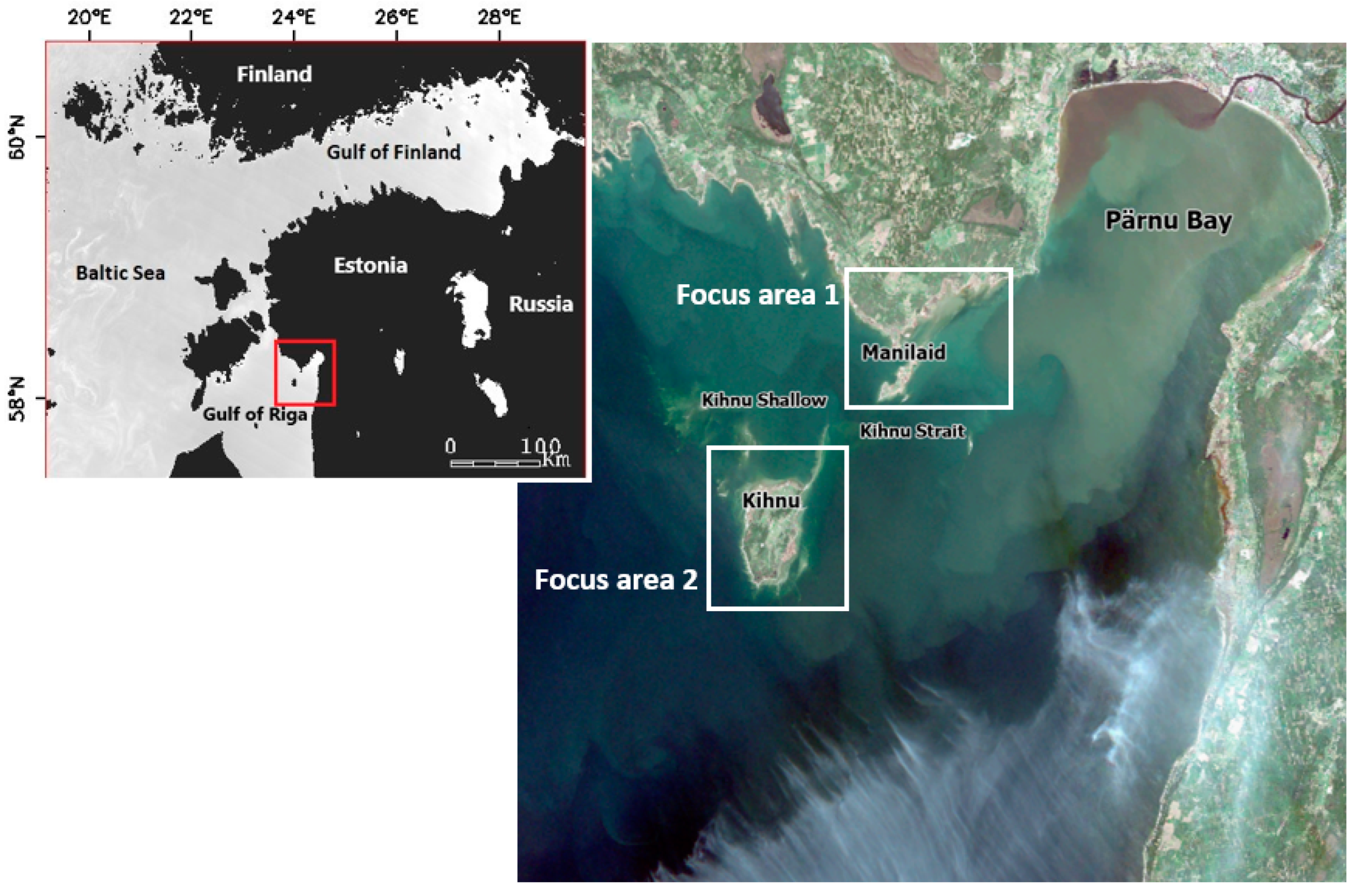
2.1. Study Area

Water is relatively turbid or highly absorbing in many parts of the brackish and non-tidal Baltic Sea, mainly due to the high amount of colored dissolved organic matter (CDOM) originating from terrestrial ecosystems. The shallow Pärnu Bay in the Gulf of Riga, the Baltic Sea (Figure 1), is highly affected by the riverine inputs, where high CDOM and particulate material fluxes are transported to the Bay through the Pärnu River. The water quality in the Bay is also affected by wind and wave action, which causes the resuspension of fine bottom sediments to the water column.
Two focus areas, representing SAV distribution hotspots with observable SAV communities, were defined in Pärnu Bay for multi-temporal SAV %cover assessment. Both focus areas were located in clearer parts of the Bay, further away from the mouth of the Pärnu River. Focus area 1 was located in a sheltered area, covering the coast of the Estonian mainland and the Manilaid Island. Focus area 2 was located in a more open part of the sea, covering the coast of Kihnu Island. The deeper Kihnu Strait is located between Kihnu Island and Manilaid Island [21]. North from the Kihnu Island is the Kihnu Shallow (benthos is observable from an S2 image (Figure 1)), which is characterized by a steep bank slope [22]. The salinity in the focus areas is low and generally varies between 3.5 and 6.5 PSU. Many freshwater species are adapted to the life in low-salinity marine waters. The dominant SAV communities in the Pärnu Bay are charophytes (Chara spp.), vascular plants (Stuckenia pectinata, Myriophyllum spicatum), filamentous green macroalgae (Cladophora glomerata) and filamentous brown macroalgae (Pylaiella littoralis).

2.2. Satellite Imagery

Archived S2 Level 1C (top of the atmosphere reflectance) data from the European Space Agency (ESA) Copernicus Open Access Hub were used for the analysis. The “best” S2 images in terms of cloud cover and water turbidity, available between 2016 and 2022 from the beginning and at the peak of the growing period, were determined and downloaded. For most of the years, at least one cloud-free or low-cloud-cover image existed per year and per season (Table 1).
The Sentinel Application Platform (SNAP) was used to resample S2 bands to the 10 m spatial resolution. All downloaded S2 images were resized to cover the study area (Figure 1). Land pixels were masked out using information from the near infrared (NIR) spectral band (S2 Band 8). In the current study, the threshold value for S2 Level 1C Band 8 was 1000. Some darker unmasked land pixels were later manually included in the mask. Additional pre-processing steps included visual inspection and manual cloud and cloud shadow masking over the water pixels. Finally, the deep water calibration (DWC) approach, implemented in the IDA image processing software [23,24], was used for atmospheric correction. High-accuracy atmospheric correction is required for physics-based bio-optical inversion models [25]. Our previous studies have shown that high-quality water surface spectra are retrieved as a result of DWC atmospheric correction [19,26]. The data visualization was performed in ENVI® image analysis and processing software.

2.3. Optically Deep Water (ODW) Mask

The ODW mask was created based on the 12th of May 2021 S2 image using a supervised classification approach [19] and used on all the collected images (Table 1). We are aware that water transparency differences can occur between different dates, so some areas could be classified either as ODW or optically shallow water (OSW) depending on the water conditions on the specific time. Still, using the same ODW mask on all the images allowed for more consistent comparison between images and saved from time-consuming processing.

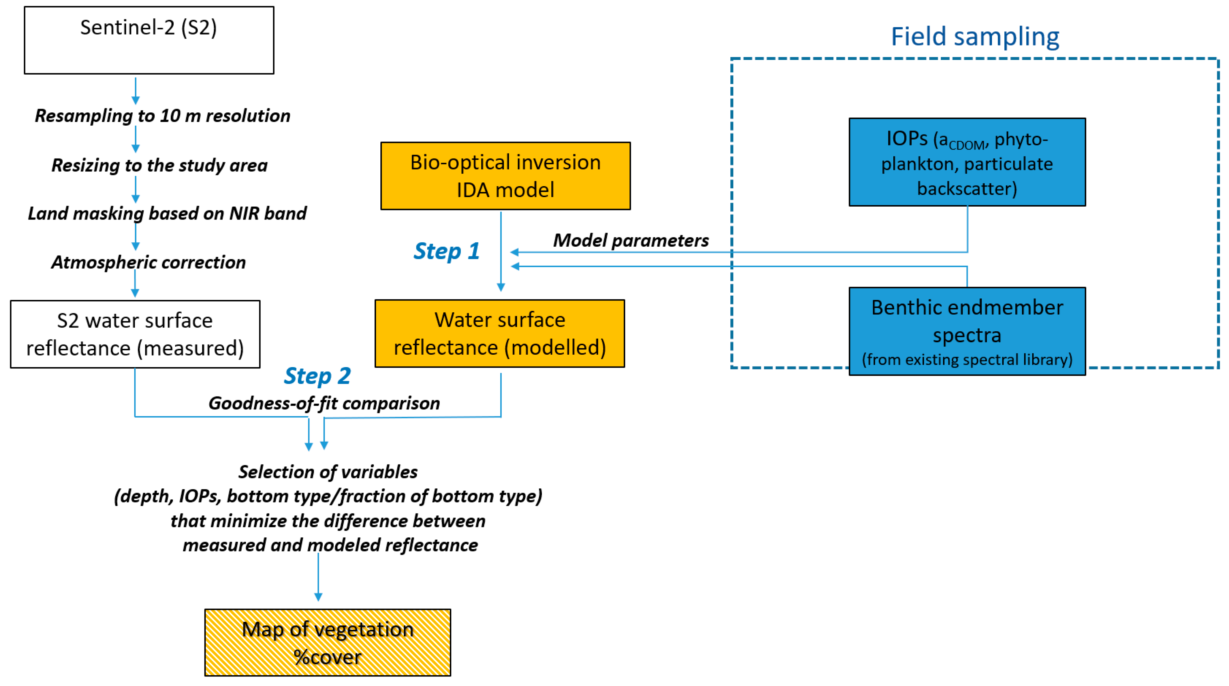
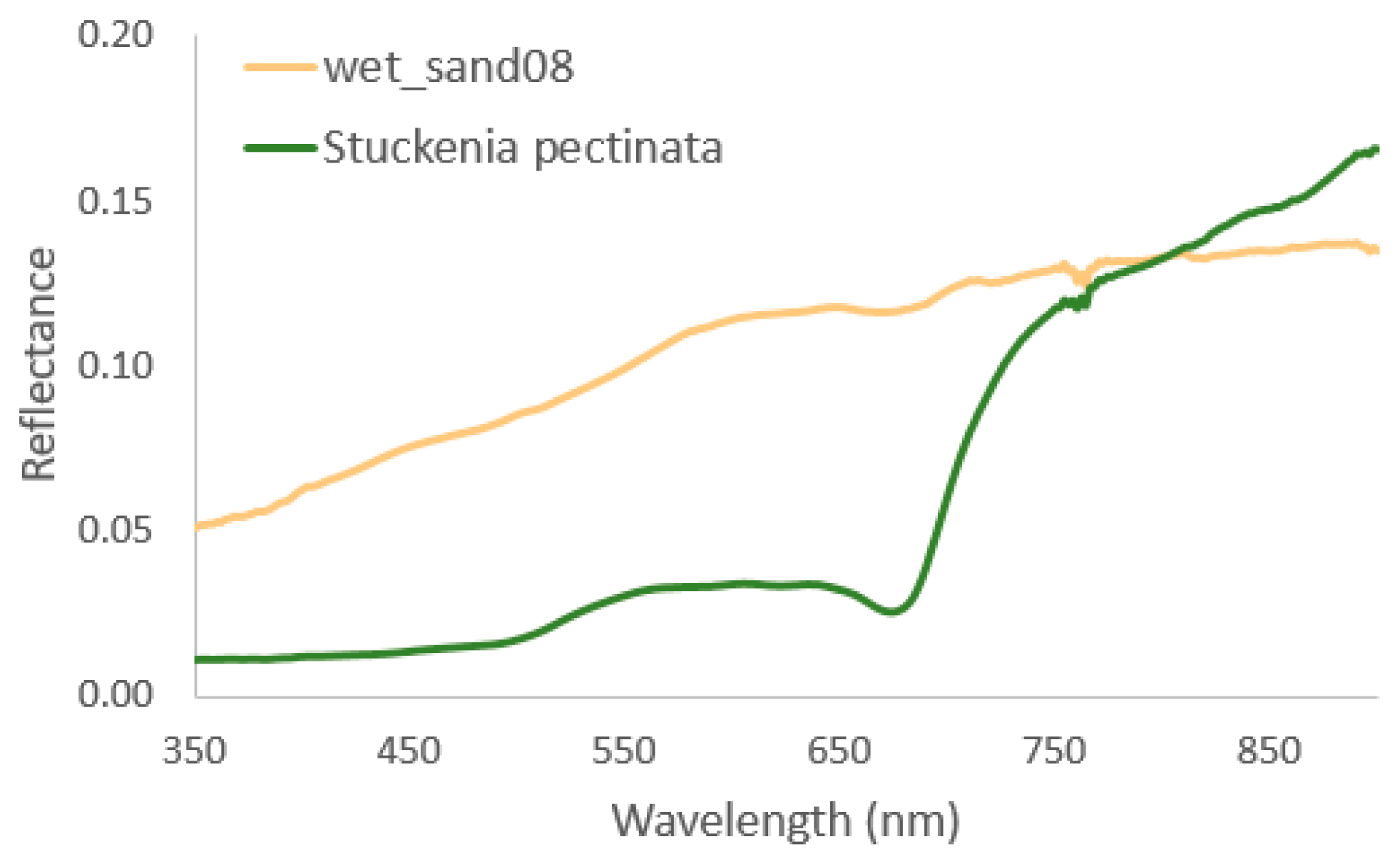
2.4. Physics-Based IDA Model

The physics-based bio-optical inversion IDA model (by Numerical Optics) was used for SAV %cover retrieval. Similar to other physics-based models (e.g., BOMBER (Bio-Optical Model-Based tool for Estimating water quality and bottom properties from remote sensing images), WASI (Water Color Simulator)), IDA simultaneously solves for different water column and benthic parameters, including the water depth and inherent optical properties (IOPs) of the water column and bottom reflectance [23,27]. In the current study, our main aim was to retrieve information about the benthic properties.
A flow chart of the methodology is provided in Figure 2. Field sampling was performed only in 2021, when water column optical properties were measured at different locations to predefine ranges for model parameterization. Additional information about the field studies, model parameterization and validation activities can be found in Ref. [19].
The first step of IDA modeling includes the forward modeling, where physics-based equations and measured water column parameters (concentrations of CDOM and phytoplankton and particulate backscatter) are used to model a large number of water surface reflectance spectra (Figure 2). Parameters, such as the water depth and IOPs, can be varied in predefined ranges during the process of forward modeling. As a second step, modeled spectra are compared with measured S2 water surface reflectance spectra (Figure 2). The selection of parameters that minimizes the difference between measured and modeled spectra are retained as a result of the comparison.
In optically shallow water, the IDA model also considers the spectral influence from the water bottom. The integration of a linear mixing model of various benthic classes within the IDA model allows us to obtain the fractional contribution of each benthic endmember to the total reflectance. Therefore, if we use endmember spectra from bare substrate and characteristic SAV species, it is possible to acquire estimates of what is the fractional contribution of SAV %cover in relation to bare substrate in each S2 image pixel.
However, previous studies have shown that physics-based models are sensitive to input parameters [20,28]. The accuracy performance of the model depends on the used benthic endmember spectra, i.e., whether they are representative of those in the study area. Validation results from the Pärnu Bay area in 2021 showed that the IDA model provided the highest performance in SAV %cover mapping if the model was parameterized with two benthic endmember spectra: wet_sand08 (bare substrate) and Stuckenia pectinata (higher plants) [19]. Therefore, in the current study, the spatiotemporal dynamics of SAV %cover over the years 2016–2021 were reconstructed using two endmember spectra: wet_sand08 and Stuckenia pectinata (Figure A1).

2.5. Area Estimates

Areal extent estimates of different SAV %cover ranges (with 10% increments) were generated by counting the pixels of each %cover range and multiplying the number with the area of the S2 pixels (10 × 10 m).

3. Results

The total surface areas of Focus areas 1 and 2 were 82 km2 and 95 km2, respectively (Table 2). Both focus areas included pixels from land, ODW and OSW (Figure 1). The same ODW mask was used on all the S2 images to allow for a more consistent comparison between years, and it covered 41.9 km2 of Focus area 1 and 49.3 km2 of Focus area 2. The land mask covered approximately 22 km2 and 18 km2, respectively. The land mask changed in size to a small extent, as the land mask was created based on the NIR band, in which case, the border between land and water was influenced by the water level (high or low water level) at the given time. As a result, the areal extent of the OSW for which the SAV %cover was assessed was approximately 19 km2 in Focus area 1 and 28 km2 in Focus area 2.

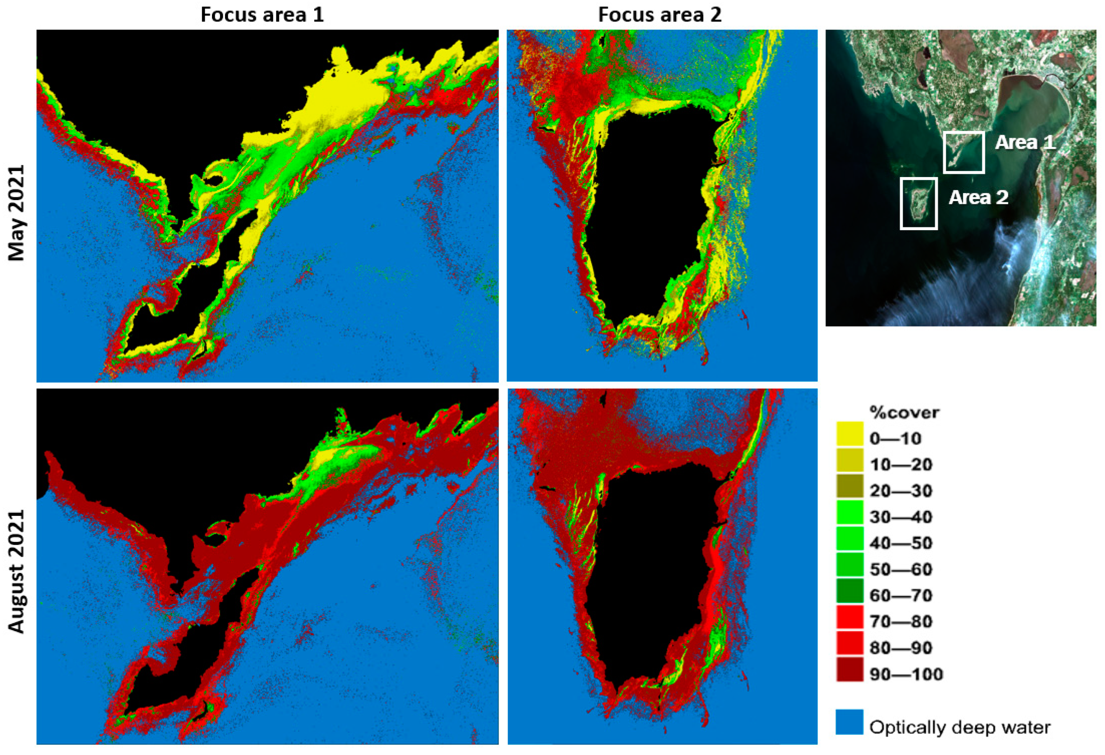
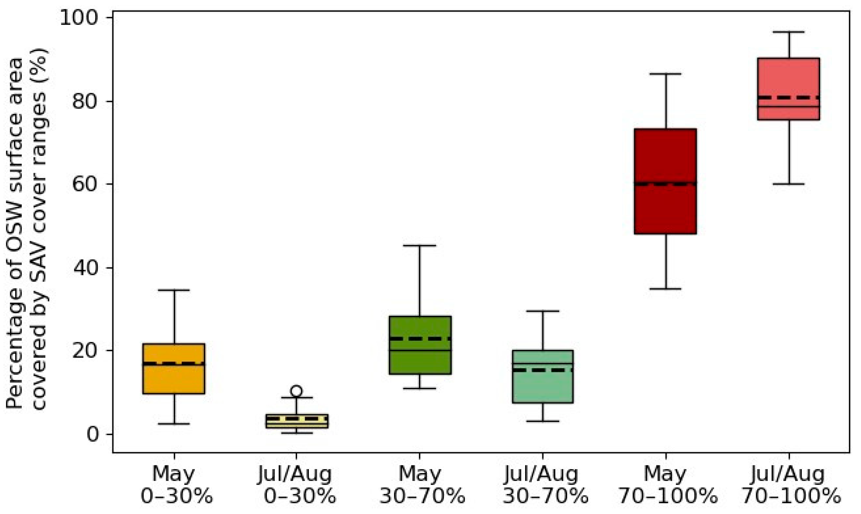
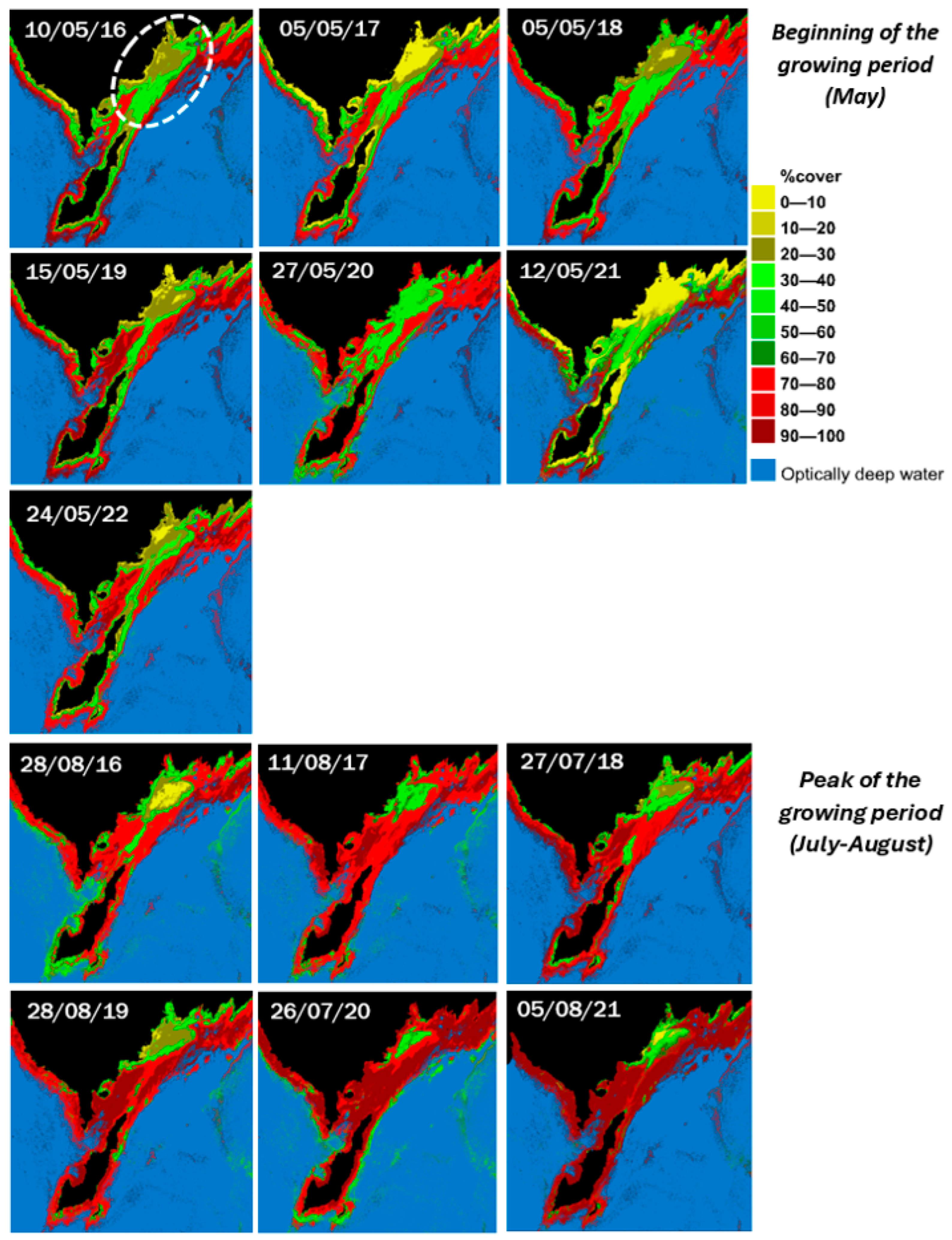
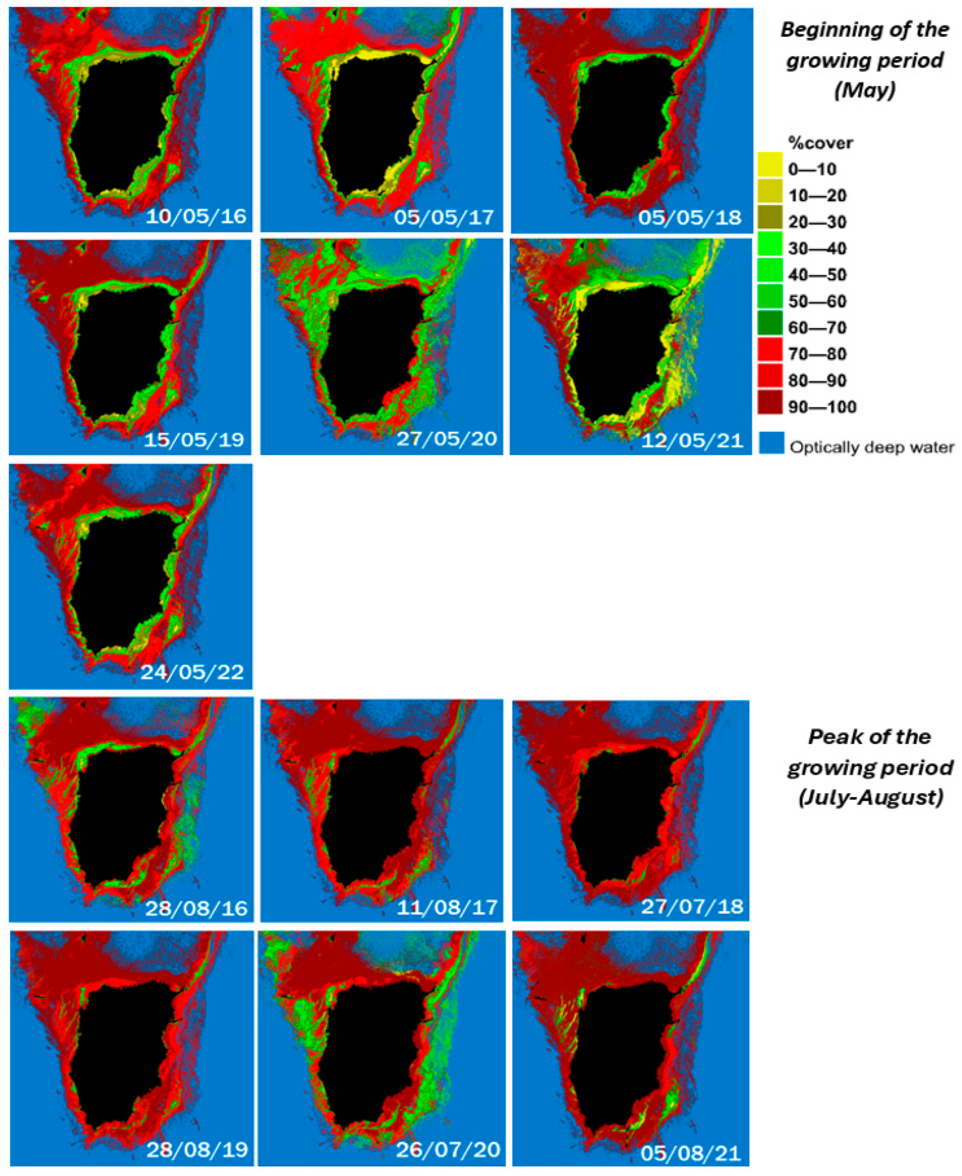
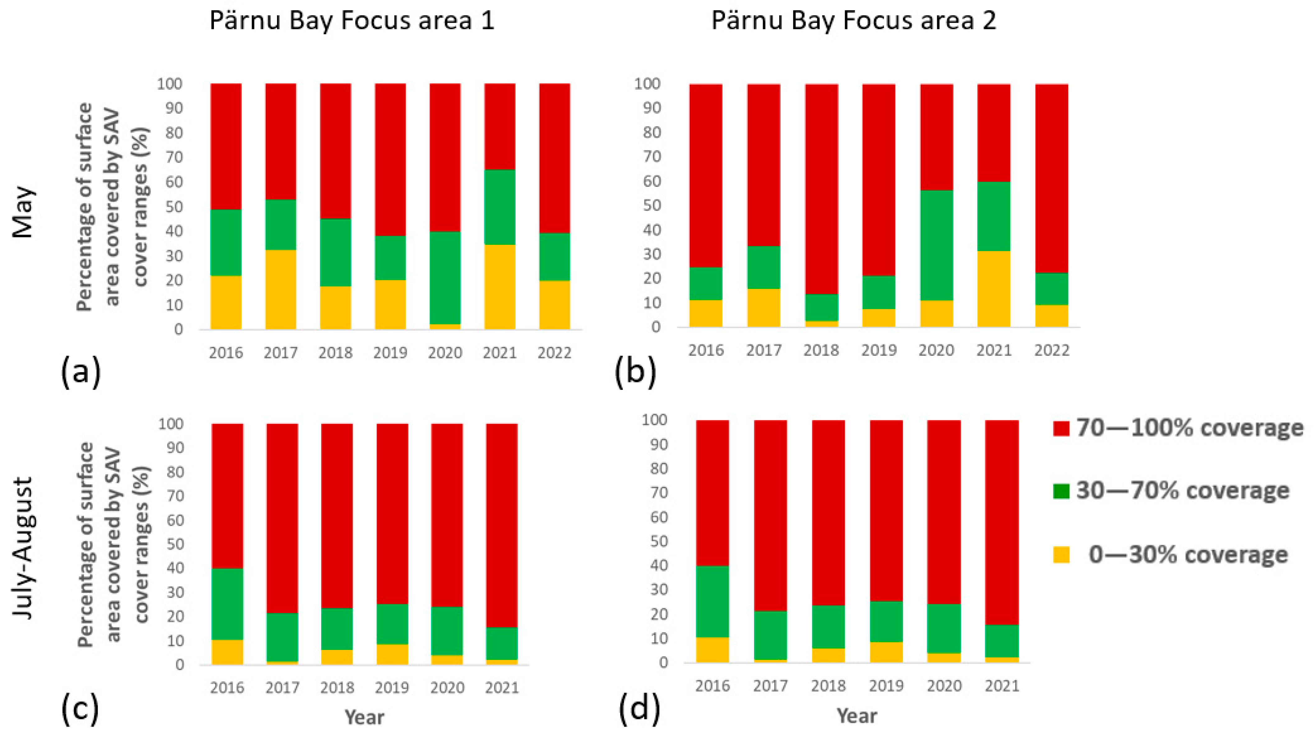
3.1. Intra-Annual Variations in SAV %Cover

Modeling results show that significant changes took place in the SAV %cover across growing periods (Figure 3). The current example shows that striking intra-annual variations exist in the SAV %cover patterns between the beginning (May 2021) and the peak of the growing period (August 2021). Considerably lower SAV %cover estimates were detected at the beginning of the vegetation period.
Intra-annual variations in the areal extent of different SAV %cover ranges between May and July/August are quantified in Figure 4. For clarity, the %cover ranges are summarized and presented as low- (0–30%), intermediate- (30–70%) and high-cover (70–100%) areas. The areal extents of the %cover ranges are given as percentages of the total OSW area (19 km2, Focus area 1 and 28 km2, Focus area 2). Each boxplot shows variability in the areal extents of three SAV cover ranges separately for both growing periods. For May, the variability in the extent of cover ranges was calculated using seven Sentinel-2 images from 2016–2022 (Table 1) and two Focus areas (14 data sets). For July/August, the variability in the extent of cover ranges was calculated using six Sentinel-2 images from 2016–2021 (Table 1) and the same two Focus areas (12 data sets).
For most of the years, a higher extent of low-cover areas was detected in May compared to in July/August. The percentage of low-cover surface areas varied in the range of 2–35% in May (mean value, 17%), and remained between 0.3 and 10% in July/August (mean value, 4%). Similarly, a higher extent of intermediate-cover level areas was detected in May compared to in July/August. The intermediate-cover area varied between 11 and 45% in May (mean value, 23%) and between 3 and 30% in July/August (mean value, 15%). Thereafter, a higher extent of high-cover areas was detected in July/August. The high-cover area varied between 35 and 86% in May (mean value, 60%) and between 60 and 97% in July/August (mean value, 81%).
In general, the extent of low-cover areas, as well as intermediate-cover areas was greater at the beginning of the vegetation period compared to that in late summer. On the contrary, the extent of high-cover areas was greater in the peak of the growing period. This indicates that low- and intermediate-cover areas decreased and high-cover areas increased during the growing period. Some low- and intermediate-cover areas became to high-cover areas during the growing period because of recolonization and vegetation growth.

3.2. Inter-Annual Variations in SAV Cover

Figure 5 and Figure 6 present SAV %cover maps for the two focus areas and two growing periods over the successive years.
Spatial patterns of SAV %cover within both growing periods underwent moderate fluctuations over the seven-year period. In Focus area 1, the vegetation patterns are relatively stable, showing low-SAV-cover areas (0–30% coverage) near shallow coastal areas in the spring (Figure 5, the area marked with the white dashed line). Those areas were later vegetated to a large extent by vascular plants such as Stuckenia pectinata, Myriophyllum spicatum and charophytes Chara spp. Focus area 2 shows some greater variability in the extents of SAV cover classes between years at the beginning of the growing period (Figure 6), while the variability diminishes by late summer.
Figure 7 displays trends in surface areal extents covered by different SAV cover ranges across the years 2016–2022 for two vegetation periods and two study scenes. The variability between years was greater in the beginning of the vegetation period, while the peak of the growing period shows greater stability in the areal extents of the cover classes. The dominant macrophyte species show much a greater salinity range [29] than that present in the focus areas. The salinity fluctuations in combination with other environmental variables cause shifts in SAV species composition but are not expected to impact the general SAV %cover [30]. Coastal benthic communities in shallow water areas in boreal environments are exposed to natural physical disturbances of varying magnitude caused mainly by storm events and ice scours [7]. These disturbances are more severe during autumn and winter. As such, the higher variability at the beginning of the vegetation period can be conditioned on the occurrence and magnitude of such natural disturbances.

4. Discussion

Our first objective was to explore the potential of S2 to map the development and expansion of SAV %cover within a SAV growing season—at the beginning and at the peak of the growing period. Another objective was to analyze whether a time-series of archived S2 data allows for the reconstruction of the spatiotemporal dynamics of SAV %cover in an inter-annual domain.
Perennial SAV species provide %cover and biomass throughout the year in the Baltic Sea [31,32], but their growing period starts in the spring, resulting in a SAV biomass maximum in the summer [33]. Although, annual fast-growing filamentous algae (such as Pylaiella littoralis, Cladophora glomerata) may be present at high densities on hard bottoms already in May, most of the dominant perennial species (such as Chara sp., Stuckenia pectinata, Myriophyllum spicatum and Potamogeton perfoliatus) are at the beginning of their natural growing period and are present at lower densities. The cover and biomass of given species increase considerably over the growing period.
In addition to the natural decaying of plants at the end of the vegetation period, physical forcing, such as intensified wave action, strong storms and seasonal ice scouring may enhance the rapid decreases in SAV cover and biomass during autumn and winter [34,35]. Shallow SAV communities are highly exposed to such disturbances in Pärnu Bay. Figure 3 shows that extensive non-vegetated areas predominate the shallow soft bottom after winter. However, most of the free space is recolonized by SAV communities by the second half of the summer. This is common in our region, as most of the species in the Baltic Sea are regarded as highly tolerant to disturbances and capable of quick recovery [7]. As a result, SAV species show high seasonal variations in cover and biomass [33]. Such intra-annual variations in SAV %cover were also well captured by S2 imagery in both focus areas in Pärnu Bay.
Our second objective was to capture the spatiotemporal dynamics of SAV %cover over successive years (2016–2022). In Focus area 1 (Figure 5), extensive low-cover areas (<30%) occurred in soft-bottomed shallows each spring, except in May 2020. As mentioned earlier, these areas are most probably subjected to physical disturbances, such as scouring by ice during the winter. Sea ice forms in Pärnu Bay annually, and the length of the ice season is between 3 and 5 months [36]. According to the Meteorological Yearbooks of Estonia, the winter in 2019/2020 was the warmest winter in Estonia since the year 1961/1962 [37]. The visual inspection of available S2 images through the Finnish Environmental Institute (SYKE) TARKKA portal [38] confirmed that unlike other years under investigation, ice formation was not detected in the winter of 2019/2020. Therefore, physical disturbances could not have happened due to the ice scouring effect this year. This can be the reason why SAV abundance was higher on soft-bottomed shallows in May 2020 (Figure 5). Nevertheless, it should be kept in mind that although the ice scouring effect was lacking in 2020, the protection from ice was also missing, and these shallow areas could have been affected by storms this winter.
SAV %cover patterns in Focus area 2 in the 2020 spring also differ from those of other years (Figure 6), showing a lower extent of low-cover areas and a higher extent of intermediate-cover areas (30–70%). However, the scarcity of low-cover areas was even more pronounced in May 2018, but it cannot be related to the lack of an ice scouring effect, as ice was detected in the winter of 2017/2018 in Focus area 2. Other strong natural disturbances, such as wave action and storms, also control the dynamics of benthic communities [39]. We can hypothesize that Focus area 1 is more influenced by the ice scouring effect than Focus area 2, as ice accumulation and the ice scouring effect is greater in more sheltered areas during ice breakup. However, the dynamics of SAV cover in relation to other disturbances (such as storms and wave action) remains beyond the scope of the current study.
Since in situ validation data were collected in May and August 2021 [19], it was possible to validate the IDA model performance only for that year. The coefficient of determination (R2) remained between 0.58 and 0.66, and the root mean square error (RMSE), between 22.11 and 28.06 depending on the growing period, which is considered a moderately good prediction performance. In Ref. [19], we compared the performances of an empirical method and physics-based IDA method. The validation results indicated that the physics-based model was able to produce comparable and even higher accuracy SAV %cover predictions than the empirical method. Empirical methods require large amounts of training data for model development and are often site and time specific. As the physics-based method does not rely on an extensive set of simultaneously collected training data, it allows for retrospective time-series analyses across multitemporal images. Therefore, the IDA physics-based model was used in the current study to model multitemporal SAV %cover across years 2016–2022. As S2 images from the past were used in the analysis, for which we did not have ground truth data, the results of the IDA modeling for those years (all except 2021) could not be validated.
During the study, it was observed that the deeper the water was, the more the IDA model began to overestimate SAV %cover. In our validation activities, only the data from the depth range of 0.1 and 2.0 m were included in the model validation, as 2.0 m was calculated as the maximum detectable depth for the SAV %cover assessment for the current study site (details in Ref. [19]). As such, all the validation activities were mostly concentrated at this depth range. The depth range > 2 m was not specifically validated in the frame of the current manuscript. However, our initial assessment showed that if the pixels below 2 m were included in the validation, then R2 decreased dramatically and, SAV %cover was largely overestimated in those deeper water pixels by the IDA model.
We tackled this problem by generating masks for ODW areas (which generally coincided with the 2 m depth limit), and SAV %cover was not predicted for those areas. However, as emphasized in Section 2.3, the ODW mask was created based on the 2021 May image, and the same mask was used on all the collected images. As such, it may be that due to differences in water transparency between different dates, the ODW mask created might not have been entirely appropriate for all the images. It means that if lower water transparency occurred at specific dates, some pixels without a detectable benthic signal (e.g., ODW pixels) remained unmasked and SAV %cover was also predicted for those pixels. As such, if darker and deeper water areas existed on the imageries, which were not masked out by the ODW mask, then the IDA model could not resolve those pixels properly and considered them dense vegetation canopies.
The majority of anthropogenic pressures, as well as climate change effects, do not emerge in such a short time period as analyzed in the current study (e.g., 7 years). However, the analyzed period allowed us to identify SAV spatiotemporal dynamics, which can further support establishing a baseline for naturally occurring variability. In this context, S2 satellite data are well suited for detecting and monitoring the seasonal and inter-annual processes of coastal SAV ecosystems. The current approach allows for the visualization and monitoring of SAV spatial patterns, as well as allowed us to quantify the surface areas of SAV abundance levels in various seasons and years. Such dynamics would be impossible to adequately capture if traditional mapping methods were used. This information can further support the systematic and cost-effective planning of ground truth mapping campaigns for more detailed data collection.

5. Conclusions

A physics-based approach was implemented on archived S2 data to the reconstruct spatiotemporal dynamics of SAV %cover, both intra- and inter-annually, over the years 2016–2022. Significant changes took place in the SAV %cover during growing seasons, when the extent of low-cover areas were reduced and high-cover areas increased. The inter-annual variability in SAV %cover patterns was greater at the beginning of the vegetation period. At the peak of the vegetation period, low-, intermediate- and high-cover areas showed generally similar areal extents over the years. The availability of light and nutrients are not generally limiting the SAV growth in shallow coastal waters. Therefore, most of the substrate is generally overgrown either by hard- or soft-bottom SAV communities by the end of the growing period. Remote sensing seems to be a suitable tool for mapping large-scale SAV %cover and offers the required means to capture SAV dynamics both inter and intra-annually, which would be impossible to adequately evaluate using traditional survey methods.

Author Contributions

Conceptualization, E.V.; methodology, E.V., L.A. and T.K.; validation, E.V.; formal analysis, E.V. and K.T.; investigation, E.V. and T.M.-R.; resources, T.K.; writing—original draft preparation, E.V.; writing—review and editing, K.T., T.M.-R. and T.K.; visualization, E.V. and K.T. All authors have read and agreed to the published version of the manuscript.

Funding

This research was funded by the Estonian Research Council, grant number PUT PRG302, and European Space Agency project “ESA Baltic Regional Initiative–Integrated Maritime and Territorial Spatial Planning”, grant number 4000133566/20/I-NB.

Data Availability Statement

Publicly available data sets were analyzed in this study. Sentinel-2 data can be found here: https://scihub.copernicus.eu/ (accessed on 2021–2022). The spectral data of benthic endmembers that were used in the IDA models are provided in the Appendix A.

Conflicts of Interest

The authors declare no conflicts of interest.

Appendix A

Figure A1. Reflectance spectra of benthic endmembers used in IDA models.
Remotesensing 16 01396 g0a1

References

  1. Macreadie, P.I.; Jarvis, J.; Trevathan-Tackett, S.M.; Bellgrove, A. Seagrasses and Macroalgae: Importance, Vulnerability and Impacts. In Climate Change Impacts on Fisheries and Aquaculture; John Wiley & Sons, Ltd.: Hoboken, NJ, USA, 2017; pp. 729–770. [Google Scholar]
  2. Cotas, J.; Gomes, L.; Pacheco, D.; Pereira, L. Ecosystem Services Provided by Seaweeds. Hydrobiology 2023, 2, 75–96. [Google Scholar] [CrossRef]
  3. Duarte, C.M. Submerged Aquatic Vegetation in Relation to Different Nutrient Regimes. Ophelia 1995, 41, 87–112. [Google Scholar] [CrossRef]
  4. Meier, H.E.M.; Andersson, H.C.; Arheimer, B.; Blenckner, T.; Chubarenko, B.; Donnelly, C.; Eilola, K.; Gustafsson, B.G.; Hansson, A.; Havenhand, J.; et al. Comparing Reconstructed Past Variations and Future Projections of the Baltic Sea Ecosystem—First Results from Multi-Model Ensemble Simulations. Environ. Res. Lett. 2012, 7, 034005. [Google Scholar] [CrossRef]
  5. Andersson, A.; Meier, H.E.M.; Ripszam, M.; Rowe, O.; Wikner, J.; Haglund, P.; Eilola, K.; Legrand, C.; Figueroa, D.; Paczkowska, J.; et al. Projected Future Climate Change and Baltic Sea Ecosystem Management. Ambio 2015, 44, 345–356. [Google Scholar] [CrossRef] [PubMed]
  6. Wikström, S.A.; Carstensen, J.; Blomqvist, M.; Krause-Jensen, D. Cover of Coastal Vegetation as an Indicator of Eutrophication along Environmental Gradients. Mar. Biol. 2016, 163, 257. [Google Scholar] [CrossRef] [PubMed]
  7. Herkül, K.; Kotta, J.; Pärnoja, M. Effect of Physical Disturbance on the Soft Sediment Benthic Macrophyte and Invertebrate Community in the Northern Baltic Sea. Boreal Environ. Res. 2011, 16, 209–219. [Google Scholar]
  8. Zhang, Q.; Xu, Y.S.; Huang, L.; Xue, W.; Sun, G.Q.; Zhang, M.X.; Yu, F.H. Does Mechanical Disturbance Affect the Performance and Species Composition of Submerged Macrophyte Communities? Sci. Rep. 2014, 4, 4888. [Google Scholar] [CrossRef] [PubMed]
  9. Kutser, T.; Hedley, J.; Giardino, C.; Roelfsema, C.; Brando, V.E. Remote Sensing of Shallow Waters—A 50 Year Retrospective and Future Directions. Remote Sens. Environ. 2020, 240, 111619. [Google Scholar] [CrossRef]
  10. Benfield, S.L.; Guzman, H.M.; Mair, J.M.; Young, J.A.T. Mapping the Distribution of Coral Reefs and Associated Sublittoral Habitats in Pacific Panama: A Comparison of Optical Satellite Sensors and Classification Methodologies. Int. J. Remote Sens. 2007, 28, 5047–5070. [Google Scholar] [CrossRef]
  11. Casal, G.; Kutser, T.; Domínguez-Gómez, J.A.; Sánchez-Carnero, N.; Freire, J. Mapping Benthic Macroalgal Communities in the Coastal Zone Using CHRIS-PROBA Mode 2 Images. Estuar. Coast. Shelf Sci. 2011, 94, 281–290. [Google Scholar] [CrossRef]
  12. Hill, V.J.; Zimmerman, R.C.; Bissett, W.P.; Dierssen, H.; Kohler, D.D.R. Evaluating Light Availability, Seagrass Biomass, and Productivity Using Hyperspectral Airborne Remote Sensing in Saint Joseph’s Bay, Florida. Estuaries Coasts 2014, 37, 1467–1489. [Google Scholar] [CrossRef]
  13. Eugenio, F.; Marcello, J.; Martin, J. High-Resolution Maps of Bathymetry and Benthic Habitats in Shallow-Water Environments Using Multispectral Remote Sensing Imagery. IEEE Trans. Geosci. Remote Sens. 2015, 53, 3539–3549. [Google Scholar] [CrossRef]
  14. Traganos, D.; Reinartz, P. Mapping Mediterranean Seagrasses with Sentinel-2 Imagery. Mar. Pollut. Bull. 2018, 134, 197–209. [Google Scholar] [CrossRef]
  15. Kuhwald, K.; Schneider von Deimling, J.; Schubert, P.; Oppelt, N. How Can Sentinel-2 Contribute to Seagrass Mapping in Shallow, Turbid Baltic Sea Waters? Remote Sens. Ecol. Conserv. 2021, 8, 328–346. [Google Scholar] [CrossRef]
  16. Ghirardi, N.; Bolpagni, R.; Bresciani, M.; Valerio, G.; Pilotti, M.; Giardino, C. Spatiotemporal Dynamics of Submerged Aquatic Vegetation in a Deep Lake from Sentinel-2 Data. Water 2019, 11, 563. [Google Scholar] [CrossRef]
  17. Fritz, C.; Kuhwald, K.; Schneider, T.; Geist, J.; Oppelt, N. Sentinel-2 for Mapping the Spatio-Temporal Development of Submerged Aquatic Vegetation at Lake Starnberg (Germany). J. Limnol. 2019, 78, 71–91. [Google Scholar] [CrossRef]
  18. Ivajnšič, D.; Orlando-Bonaca, M.; Donša, D.; Grujić, V.J.; Trkov, D.; Mavrič, B.; Lipej, L. Evaluating Seagrass Meadow Dynamics by Integrating Field-Based and Remote Sensing Techniques. Plants 2022, 11, 1196. [Google Scholar] [CrossRef] [PubMed]
  19. Vahtmäe, E.; Toming, K.; Argus, L.; Möller-Raid, T.; Ligi, M.; Kutser, T. On the Possibility to Map Submerged Aquatic Vegetation Cover with Sentinel-2 in Low-Transparency Waters. J. Appl. Remote Sens. 2023, 17, 044506. [Google Scholar] [CrossRef]
  20. Dekker, A.G.; Phinn, S.R.; Anstee, J.; Bissett, P.; Brando, V.E.; Casey, B.; Fearns, P.; Hedley, J.; Klonowski, W.; Lee, Z.P.; et al. Intercomparison of Shallow Water Bathymetry, Hydro-Optics, and Benthos Mapping Techniques in Australian and Caribbean Coastal Environments. Limnol. Oceanogr. Methods 2011, 9, 396–425. [Google Scholar] [CrossRef]
  21. Suursaar, Ü.; Kullas, T.; Otsmann, M. Flow Modelling in the Pärnu Bay and the Kihnu Strait. Proc. Est. Acad. Sci. Eng. 2002, 8, 189–203. [Google Scholar]
  22. Kotta, J.; Lauringson, V.; Martin, G.; Simm, M.; Kotta, I.; Herkül, K.; Ojaveer, H. Gulf of Riga and Pärnu Bay. In Ecology of Baltic Coastal Waters; Schiewer, U., Ed.; Springer: Berlin/Heidelberg, Germany, 2008; pp. 217–243. [Google Scholar]
  23. Hedley, J.D.; Roelfsema, C.; Brando, V.; Giardino, C.; Kutser, T.; Phinn, S.; Mumby, P.J.; Barrilero, O.; Laporte, J.; Koetz, B. Coral Reef Applications of Sentinel-2: Coverage, Characteristics, Bathymetry and Benthic Mapping with Comparison to Landsat 8. Remote Sens. Environ. 2018, 216, 598–614. [Google Scholar] [CrossRef]
  24. Casal, G.; Hedley, J.D.; Monteys, X.; Harris, P.; Cahalane, C.; McCarthy, T. Satellite-Derived Bathymetry in Optically Complex Waters Using a Model Inversion Approach and Sentinel-2 Data. Estuar. Coast. Shelf Sci. 2020, 241, 10681. [Google Scholar] [CrossRef]
  25. Goodman, J.A.; Lee, Z.P.; Ustin, S.L. Influence of Atmospheric and Sea-Surface Corrections on Retrieval of Bottom Depth and Reflectance Using a Semi-Analytical Model: A Case Study in Kaneohe Bay, Hawaii. Appl. Opt. 2008, 47, F1–F11. [Google Scholar] [CrossRef]
  26. Vahtmäe, E.; Kotta, J.; Lõugas, L.; Kutser, T. Mapping Spatial Distribution, Percent Cover and Biomass of Benthic Vegetation in Optically Complex Coastal Waters Using Hyperspectral CASI and Multispectral Sentinel-2 Sensors. Int. J. Appl. Earth Obs. Geoinf. 2021, 102, 102444. [Google Scholar] [CrossRef]
  27. Hedley, J.; Roelfsema, C.; Phinn, S.R. Efficient Radiative Transfer Model Inversion for Remote Sensing Applications. Remote Sens. Environ. 2009, 113, 2527–2532. [Google Scholar] [CrossRef]
  28. Garcia, R.A.; Lee, Z.; Hochberg, E.J. Hyperspectral Shallow-Water Remote Sensing with an Enhanced Benthic Classifier. Remote Sens. 2018, 10, 147. [Google Scholar] [CrossRef]
  29. Herkül, K.; Torn, K.; Möller-Raid, T.; Martin, G. Distribution and Co-Occurrence Patterns of Charophytes and Angiosperms in the Northern Baltic Sea. Sci. Rep. 2023, 13, 147. [Google Scholar] [CrossRef]
  30. Kovtun, A.; Torn, K.; Kotta, J. Long-Term Changes in a Northern Baltic Macrophyte Community. Est. J. Ecol. 2009, 58, 270–285. [Google Scholar] [CrossRef]
  31. Kraufvelin, P.; Salovius, S. Animal Diversity in Baltic Rocky Shore Macroalgae: Can Cladophora Glomerata Compensate for Lost Fucus Vesiculosus? Estuar. Coast. Shelf Sci. 2004, 61, 369–378. [Google Scholar] [CrossRef]
  32. Kotta, J.; Torn, K.; Paalme, T.; Rätsep, M.; Kaljurand, K.; Teeveer, M.; Kotta, I. Scale-Specific Patterns of the Production of the Charophyte Chara Aspera in the Brackish Baltic Sea: Linking Individual and Community Production and Biomass Growth. Front. Mar. Sci. 2021, 8, 674014. [Google Scholar] [CrossRef]
  33. Jankowska, E.; Włodarska-Kowalczuk, M.; Kotwicki, L.; Balazy, P.; Kuliński, K. Seasonality in Vegetation Biometrics and Its Effects on Sediment Characteristics and Meiofauna in Baltic Seagrass Meadows. Estuar. Coast. Shelf Sci. 2014, 139, 159–170. [Google Scholar] [CrossRef]
  34. Jerker, I.-A. Dynamics of Submerged Aquatic Vegetation on Shallow Soft Bottoms in the Baltic Sea. J. Veg. Sci. 2000, 11, 425–432. [Google Scholar] [CrossRef]
  35. Paar, M.; Berthold, M.; Schumann, R.; Dahlke, S.; Blindow, I. Seasonal Variation in Biomass and Production of the Macrophytobenthos in Two Lagoons in the Southern Baltic Sea. Front. Earth Sci. 2021, 8, 542391. [Google Scholar] [CrossRef]
  36. Wang, K.; Leppäranta, M.; Kõuts, T. A Study of Sea Ice Dynamic Events in a Small Bay. Cold Reg. Sci. Technol. 2006, 45, 83–94. [Google Scholar] [CrossRef]
  37. Meteorological Yearbooks of Estonia. Available online: https://www.ilmateenistus.ee/ilmatarkus/publikatsioonid/aastaraamatud/ (accessed on 20 December 2023).
  38. Finnish Environmental Institute. (SYKE) TARKKA Portal. Available online: https://wwwi4.ymparisto.fi/i4/fin/tarkka (accessed on 20 December 2023).
  39. Herkül, K.; Kotta, J.; Kotta, I.; Orav-Kotta, H.; Herkül, K.; Kotta, J.; Kotta, I.; Orav-Kotta, H. Effects of Physical Disturbance, Isolation and Key Macrozoobenthic Species on Community Development, Recolonisation and Sedimentation Processes. Oceanologia 2006, 48, 267–282. [Google Scholar]
Figure 1. Location of the study areas in the Gulf of Riga (red rectangle), the Baltic Sea. The specific focus areas are projected on the Sentinel-2 imagery acquired on the 12th of May 2021.
Remotesensing 16 01396 g001
Figure 2. Flow chart of the methodology used in the current study for mapping SAV %cover.
Remotesensing 16 01396 g002
Figure 3. Examples of landscape-scale SAV %cover maps obtained using physics-based IDA model for two focus areas in the beginning (May 2021) and at the peak of the growing period (August 2021).
Remotesensing 16 01396 g003
Figure 4. Intra-annual variations in the areal extent of SAV %cover ranges (0–30%, 30–70% and 70–100% coverage), all years combined and over both focus areas in Pärnu Bay. Upper whisker—maximum; lower whisker—minimum; line—median; dashed line—mean; circles—outliers; box—interquartile range. OSW—optically shallow water.
Remotesensing 16 01396 g004
Figure 5. SAV %cover maps acquired using physics-based IDA model for Focus area 1 across the years 2016–2022. Low %cover areas in soft-bottomed shallows are indicated with white dashed lines.
Remotesensing 16 01396 g005
Figure 6. SAV %cover maps acquired using physics-based IDA model for Focus area 2 across the years 2016–2022.
Remotesensing 16 01396 g006
Figure 7. Trends in the areal extent of %cover ranges across years for two vegetation periods (beginning and peak of the growing period) and two focus areas in Pärnu Bay: (a) Focus area 1 in May, (b) Focus area 2 in May, (c) Focus area 1 in July-August, (d) Focus area 2 in July-August.
Remotesensing 16 01396 g007
Table 1. Dates of the S2 images that were downloaded from the ESA Copernicus Open Access Hub and used for retrospective SAV cover analysis.
Beginning of the
Growing Period
Peak of the
Growing Period
5 May 201628 August 2016
5 May 201711 August 2017
5 May 201827 July 2018
15 May 201928 August 2019
27 May 202026 July 2020
12 May 20215 August 2021
24 May 2022-
Table 2. The surface areas of both study scenes covered by optically shallow water (OSW) and masked out by land and optically deep water (ODW) masks.
Focus Area 1Focus Area 2
Total surface area83 km295 km2
Land mask* 22 km2* 18 km2
ODW mask42 km249 km2
OSW area19 km228 km2
* Changed in size to a small extent depending on the water level.
Disclaimer/Publisher’s Note: The statements, opinions and data contained in all publications are solely those of the individual author(s) and contributor(s) and not of MDPI and/or the editor(s). MDPI and/or the editor(s) disclaim responsibility for any injury to people or property resulting from any ideas, methods, instructions or products referred to in the content.

