
Long-Tailed Effect Study in Remote Sensing Semantic Segmentation Based on Graph Kernel Principles
by
 ,
,
Wei Cui
1,*,
Zhanyun Feng
1,
Jiale Chen
1,
Xing Xu
1,
Yueling Tian
1,
Huilin Zhao
2 and
Chenglei Wang
1 1
School of Resources and Environmental Engineering, Wuhan University of Technology, Wuhan 430070, China
2
Department of Land Surveying and Geo-Informatics, Hong Kong Polytechnic University, Hong Kong
*
Author to whom correspondence should be addressed.
Remote Sens. 2024, 16(8), 1398; https://doi.org/10.3390/rs16081398
Submission received: 29 February 2024
/
Revised: 12 April 2024
/
Accepted: 12 April 2024
/
Published: 15 April 2024
Abstract
:The performance of semantic segmentation in remote sensing, based on deep learning models, depends on the training data. A commonly encountered issue is the imbalanced long-tailed distribution of data, where the head classes contain the majority of samples while the tail classes have fewer samples. When training with long-tailed data, the head classes dominate the training process, resulting in poorer performance in the tail classes. To address this issue, various strategies have been proposed, such as resampling, reweighting, and transfer learning. However, common resampling methods suffer from overfitting to the tail classes while underfitting the head classes, and reweighting methods are limited in the extreme imbalanced case. Additionally, transfer learning tends to transfer patterns learned from the head classes to the tail classes without rigorously validating its generalizability. These methods often lack additional information to assist in the recognition of tail class objects, thus limiting performance improvements and constraining generalization ability. To tackle the abovementioned issues, a graph neural network based on the graph kernel principle is proposed for the first time. By leveraging the graph kernel, structural information for tail class objects is obtained, serving as additional contextual information beyond basic visual features. This method partially compensates for the imbalance between tail and head class object information without compromising the recognition accuracy of head classes objects. The experimental results demonstrate that this study effectively addresses the poor recognition performance of small and rare targets, partially alleviates the issue of spectral confusion, and enhances the model’s generalization ability.
1. Introduction
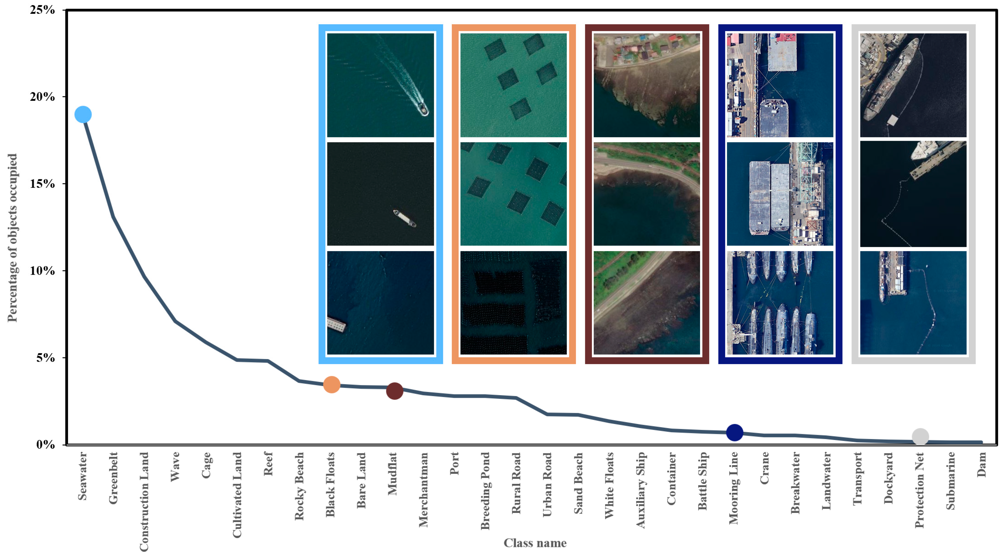
The distribution of different classes of geographical objects often exhibits a characteristic of imbalance, naturally leading to the manifestation of long-tailed distributions in many datasets [1,2]. In these datasets, head classes typically have a large number of samples, while the tail classes are characterized by a comparatively lower sample count [3]. During the training process, influenced by the dominance of quantity, deep neural network models typically perform better in learning and recognizing head classes. Conversely, tail classes struggle to achieve effective learning and recognition due to their scarce sample counts. Semantic segmentation, a key task in computer vision, is affected by the long-tailed phenomenon, where certain classes are underrepresented in the data. To visually demonstrate this long-tailed distribution, we provide an illustrative diagram of long-tailed datasets (as shown in Figure 1).
Many researchers have made enthusiastic attempts to address the problem of identifying long-tailed data. Numerous strategies such as resampling [4,5,6,7,8], reweighting [9,10,11], and transfer learning [12,13,14,15,16,17] have been successfully explored to address the issue of class imbalance. Resampling strategies aim to address the issue of data imbalance, mainly including oversampling, undersampling, and hybrid sampling [18]. Oversampling or undersampling may lead to overfitting or underfitting issues, with the risk of overfitting on the tail classes when the tail class samples are frequently oversampled, resulting in weaker generalization [5,19]. Reweighting methods are relatively lightweight and can be easily integrated into various frameworks, their effectiveness is limited, especially in highly imbalanced scenarios [20]. Transfer learning endeavors to transfer features from head classes to representations and predictions of tail classes. However, the knowledge obtained from head classes may not necessarily match the actual features of tail classes.
These methods have not further specifically extracted effective information for tail classes, addressing the issue of insufficient information in tail classes. Therefore, a more effective solution for long-tailed effect is to supplement additional information for tail classes to compensate for the insufficient information in these classes. Graph kernel enables the introduction of subgraph structural information derived by the tail objects and their neighboring nodes to enrich the information of tail classes, thus achieving information balance between tail and head classes. This study proposes a new method to address the long tail effect based on the graph kernel method. Next, we will introduce the related research of graph kernel.
In geographical scenarios, different classes of remote sensing objects often exhibit certain stable relationships with each other [21,22]. In this study, based on the statistical analysis of the dataset, we outline the stable relationships of each class, referred to as the eigenstructure. In subsequent methods, during the training process, we apply a graph kernel function to measure the similarity between the subgraphs of samples and the eigenstructure corresponding to that class, thereby assessing the effectiveness of the model in learning object structural information.
To address the challenges posed by long-tailed datasets, this paper proposes a graph neural network based on graph kernel principles applied to remote sensing semantic segmentation tasks. It leverages graph kernels to extract graph structure information from the tail class objects and their neighboring nodes, which serves as supplementary and enhancing information about the environment beyond basic visual features. Through this approach, we are able to partially compensate for the information imbalance between tail and head classes.
The main contributions of this work are as follows:
- A mechanism for representing the structural features of tail classes is proposed for the first time. By recognizing and extracting the eigenstructures of tail classes objects as supplementary information, the information imbalance between tail and head classes is alleviated.
- To further optimize the model’s training process, graph kernel is incorporated into our model, which dynamically adjusts the effect of graph structure information within the loss function, avoiding excessive suppression of head class objects and the information imbalance between head and tail classes.
- A remote sensing image semantic segmentation model based on graph kernel principles and graph neural networks (GKNNs) is designed on the basis of the aforementioned contributions to address the challenge of recognizing specific remote sensing objects of importance that are scarce and small in scale.
2. Related Work
2.1. Long-Tailed Visual Recognition
Long-tailed datasets introduce significant bias in the recognition of tail classes in deep learning models [1,23], which attracts widespread attention and research interest from scholars. The current solutions primarily focus on addressing the impact of class imbalance and can be broadly categorized into the following directions:
Resampling. Researchers have proposed some resampling strategies to directly alter the imbalanced distribution presented by the data, such as random oversampling, undersampling, and class-balanced sampling [4,5]. Oversampling involves increasing the number of minority class samples by replication or synthesis techniques such as SMOTE and Borderline-SMOTE [6,24]. Undersampling, on the other hand, reduces the number of majority class samples by randomly deleting or selectively removing samples far from the decision boundary. Chang et al. [25] proposed a joint resampling strategy, RIO. Wei [26] introduced open-sampling, a method that leverages out-of-distribution data to rebalance class priors and encourage separable representations. Yu et al. [27] revived the use of balanced undersampling, achieving higher accuracy for worst-performing categories. The method of resampling was proposed as early as the era of machine learning, constituting a traditional strategy. Solely undersampling the head classes or oversampling the tail classes without introducing new features inevitably leads to underfitting or overfitting issues, resulting in weak model generalization capability.
Reweighting (cost-sensitive methods). The literature has introduced a variety of cost-sensitive loss functions to adjust the weighting of majority and minority instances [11,20,28,29,30,31]. These methods enhance the model’s attention towards the tail classes by assigning appropriate loss weights to head and tail classes, such as adjusting the loss based on class frequencies, sample difficulty, distances to centroids, or class margins. Fernando [30] introduced a dynamically weighted balanced loss function for deep learning, which self-adapts its weights based on class frequency and predicted probability. AdaCost algorithm [28] incorporates misclassification costs into the weight update rules of the Boosting algorithm, improving its recall and precision for tail classes.
Transfer learning. Due to the differences in both the characteristics and sample size between tail and head classes, many researchers are dedicated to extracting knowledge from head classes and transferring it to tail classes to mitigate this imbalance. Wang et al. [12] introduced a meta-network that dynamically transfers meta-knowledge from head to tail classes. GistNet [13] combines random sampling loss with class-balanced sampling loss to transfer geometric information from the head to the tail. The LFME framework proposed by Xiang et al. [32] trains more balanced “Expert” models through multiple subsets and adaptively transfers knowledge to the “Student” model. With the introduction of transfer learning methods, it becomes possible to transfer knowledge from head classes to tail classes. However, further validation is required to assess whether the knowledge distilled from the head classes aligns with the actual tail classes.
2.2. Graph Kernel
Graphs are data structures composed of nodes and the edges that connect these nodes. Typically, a graph can be defined as , where represents the set of nodes and represents the set of edges. Nodes represent entities or objects, while edges represent the relationships between nodes. Graph kernel is a method used to compute the similarity of graphs, originating from the research by David Haussler et al. in 1999 [33], which first introduces the concept of kernel functions and applies convolution kernels on discrete structures.
Based on the differences in the decomposition of graphs when computing graph similarity, common graph kernel methods can be categorized into three types: path-based graph kernels, subgraph-based graph kernels, and subtree-based graph kernels. Among them, the path-based graph kernel, such as the random walk kernel [34,35], measures the similarity between graphs by calculating the common paths; the subgraph-based graph kernel [34,36] calculates the similarity between graphs by comparing the similarity of substructures within the graphs, for example, the graphlet kernel [36] measures the similarity between graphs by comparing the distributions of all possible k-node subgraphs (referred to as graphlets) within the graphs; the subtree-based graph kernel, such as the WL kernel [37], based on the similarity of subtrees, captures local structural information by iteratively labeling and aggregating nodes. These methods are commonly used for graph classification and matching.
The application of graph kernels in graph neural networks aims to enhance model recognition performance. KCNNs [38] embed local neighborhood features of graphs using graph kernels, while GNTK [39], as an extension of infinite-width GNNs, combines the expressiveness of GNNs with the advantages of graph kernels. Feng et al. [40] proposed KerGNNs, which enhance the representation capability of GNNs by integrating random walk kernel and trainable latent graphs as graph filters.
The graph kernel method provides a means for quantitatively measuring the effectiveness of the model in learning environmental structural information, enabling the model to acquire additional prior knowledge about tail classes, and further balancing the disparity in feature quantities between the head and tail.
3. Materials and Methods
This section begins by providing an overview of the network architecture of the model. In Section 3.2, we delve into the design of the structural information enhancement module and its pivotal role in the model. Finally, in Section 3.3, we provide a detailed introduction to the graph kernel structural loss function, elucidating how to dynamically adjust the structural loss to achieve optimal model performance.
3.1. The GKNNs Model Architecture
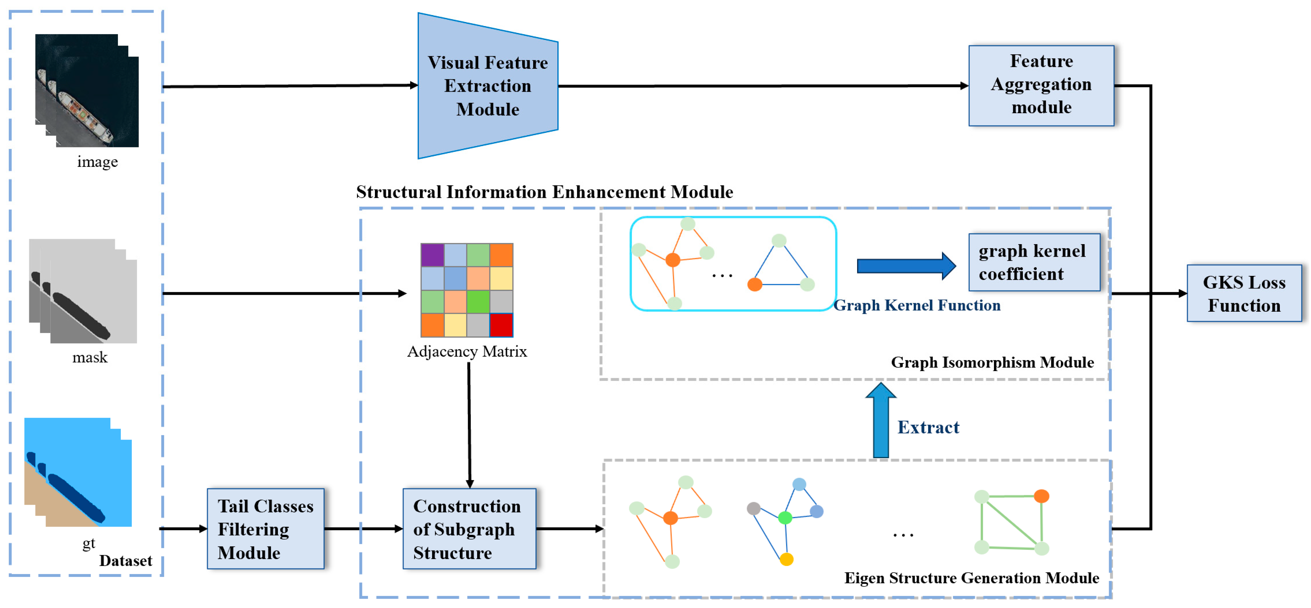
We propose a remote sensing semantic segmentation model based on graph kernel principles and graph neural networks (GKNNs), with the model architecture illustrated in Figure 2. When training remote sensing long-tailed datasets, GKNNs is able to augment the structural information of tail classes and achieve information balance with head classes, thereby improving the recognition performance of tail classes.
The model mainly consists of four modules: the visual feature extraction module, the feature aggregation module, the tail classes filtering module, and the structural information enhancement module.
The visual feature extraction module and feature aggregation module are jointly completed by the backbone network and GAT (graph attention network). The backbone network adopts ResNet34. Considering that objects of tail classes in long-tailed datasets usually have small areas, to avoid smoothing their features, we select a 112 × 112 feature map as the input for GAT and combine it with object masks to obtain aggregated object features. The tail classes filtering module is designed for selecting tail class objects that require information augmentation within a threshold, which only sends the tail classes objects to the subsequent structural information enhancement module. The structural information enhancement module is designed to enhance structural information for tail classes. In the structural information enhancement module, we initially generate neighborhood structural subgraphs for each object, followed by the extraction of the eigenstructure of the tail classes. Subsequently, the graph kernel algorithm is utilized to compute the similarity between the eigenstructure and the neighborhood subgraphs of the tail class objects.
The detailed explanation of structural information enhancement module is provided in Section 3.2. During training, we introduce a loss function called the graph kernel structural loss function, and its detailed explanation is provided in Section 3.3.
3.2. Structural Information Enhancement Module
The structural information enhancement module is specifically designed to address the issue of identifying tail classes in long-tailed distribution datasets with relatively few training samples and weak model attention. Its main purpose is to provide additional structural enhancement for these tail classes. This module mainly consists of two core components: eigenstructure generation and graph isomorphism between eigenstructure and one-hop neighborhood subgraph of the target node.
3.2.1. The Eigenstructure Generation Algorithm
The tail class filtering module filters out objects belonging to tail classes that require special attention. Subsequently, by extracting the neighborhood subgraph structures of these objects, we generate the neighborhood subgraph structure of the central object. This structure not only contains spatial relationships between the central object and its neighboring nodes, but also encompasses relationships among the neighboring nodes themselves. These neighborhood subgraph structures are then fed into the tail class eigenstructure generation module which outputs the eigenstructures of the target tail classes, representing the core and representative structural features. The eigenstructures will serve as supplementary information for tail classes, compensating for the information imbalance with head classes. Algorithm 1, shown below, elaborates on the generation process of the eigenstructure.
| Algorithm 1 Generating Eigenstructures for Tail Class |
| Input: Dataset . Set of all Tail Classes |
| ▷ Sample Ground Truth: . Adjacency Matrix: . Object Mask: |
Output:
|
| ▷ Retrieve the first-order neighboring nodes of the target object along with their adjacency relationships |
|
| ▷ Extracting the subgraph of the tail class object |
|
|
|
|
The eigenstructure refers to the collective characteristic structure of a certain class. In order to incorporate it as supplementary information into the model’s loss function, it is necessary to quantitatively describe its similarity to the subgraph composed of instances of this class and their one-hop neighboring nodes. Therefore, we design a graph isomorphism algorithm.
3.2.2. The Graph Isomorphism Algorithm of Subgraph Structure
We utilize the graph isomorphism algorithm of subgraph structure to compute the graph kernel coefficient between the one-hop neighborhood subgraph structure of the target object and its eigenstructure. The pseudocode of the algorithm is shown below. This process aims to quantify the similarity between the two structures, providing a crucial component for subsequent loss function computation. This approach effectively enhances the structural features of tail classes during training, thereby better compensating for the information imbalance between tail and head class.
In the next section, we will provide a detailed explanation of the graph kernel structural loss function proposed in this paper. This function will incorporate the aforementioned structural enhancement module to collectively improve the overall performance of the model on long-tailed distribution datasets.
3.3. Structural Loss Function
This subsection provides a detailed explanation of the definitions, computation processes, and roles of two proposed loss functions in this study, namely, the class-balanced structural loss (CBS loss) and the graph kernel structural loss (GKS loss). They both aim to incorporate structural information into the loss function. Specifically, the GKS loss, built upon the CBS loss, introduces an adaptive dynamic adjustment mechanism dependent on the eigenstructure, allowing for dynamic adjustment of the role of structural information in the loss function, thus further enhancing the model’s performance.
3.3.1. Class-Balanced Structural Loss
The design of the class-balanced structural loss aims to address the challenge of insufficient sample weights and lack of information in tail class samples in long-tailed distribution. In the traditional model training process, due to the considerably fewer samples in tail classes compared to head classes, these tail classes often fail to receive sufficient attention from the model. Coupled with the inadequate feature representation of tail classes, this results in significantly lower recognition performance for tail classes compared to head classes, known as the “long-tailed effect” [23].
For an object-based semantic segmentation model, given a sample containing multiple objects, with the ground truth label for one object and the model’s predicted probability distribution , the calculation of CBS loss for a batch of samples inputted into the model is as follows:
As shown in Equation (1), it comprises two components: the loss of all objects and the tail structural loss . The CBS loss function is improved upon the cross-entropy loss function, which is widely used in training models for classification tasks in deep learning.
measures the discrepancy between the overall sample model predicted probability distribution and the true labels. In Equation (2), represents the probability of class c in the true label of the -th object, where ∈ {1, 2,…, }, denotes the number of categories. It is typically a one-hot encoded vector where the element corresponding to the true label class is 1 and all other elements are 0, indicating the true label of the object. represents the probability of class c in the predicted probability distribution for the -th object. denotes the loss value of object , and represents the total number of objects in a training batch inputted into the model.
evaluates the prediction performance of tail classes. It incorporates the structural information of the one-hop neighbor nodes of the tail class central objects to enhance the prediction effectiveness of tail classes. In Equation (3), represents the total number of tail class objects and their one-hop neighbor objects addressed, where refers to a specific object within the scope of , and represents the loss value of object.
During training, minimizing the CBS loss function helps the model’s predictions to closely match the true labels and enhances the model’s attention towards tail classes, thereby improving the classification accuracy of tail classes.
3.3.2. Graph Kernel Structural Loss
The CBS loss aims to enhance the classification effectiveness of tail classes by strengthening the structural information of tail-class objects and reweighting them. However, due to its emphasis on the importance of tail classes, the CBS loss may affect the overall classes, especially the head classes. To address this issue and achieve balanced enhancement of both tail and head class recognition, thereby ensuring overall balance, we propose an adaptive tail structural enhancement loss function based on the graph kernel principle, termed graph kernel structural loss (GKS loss). The calculation formula of GKS loss is shown in below.
Like CBS loss, GKS loss consists of two components: the loss of all objects and the tail structural loss . The difference between CBS loss and GKS loss is the introduction of the graph kernel coefficient in the calculation of the structural loss of the tail class. The calculation process of is as follows.
In Equation (5), represents the graph kernel value between the neighborhood subgraph structure of the target object and its eigenstructure to enhance eigenstructure information. The term encompasses two types of information: sample context and eigenstructure. The sample context involves the error of the central object in the tail classes and its one-hop neighbor nodes, serving as a structural loss term to provide sample context information for tail classes training. The calculation formula for the graph kernel coefficient is shown below.
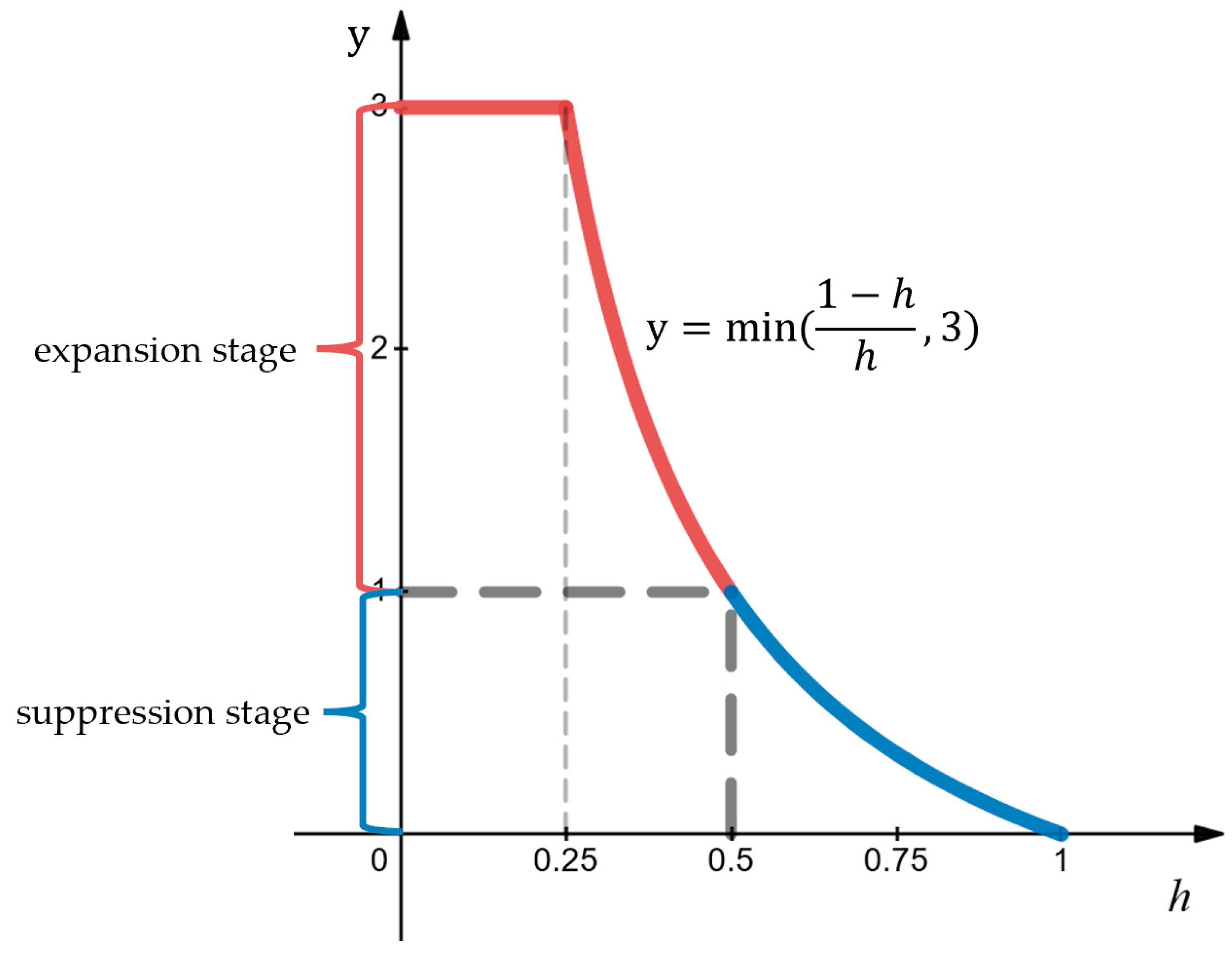
In Equation (6), refers to the neighborhood subgraph of the central object, refers to the eigenstructure of the central object class, and denotes Algorithm 2 in the structural information enhancement module, specifically the graph isomorphism algorithm between eigenstructures and neighborhood subgraphs of tail classes. The eigenstructure information, computed based on Algorithm 2 from the dataset, surpasses the contextual information contained in individual samples, providing stable eigenstructural features of target objects to control the interference caused by specific sample atypical environments. The relationship between the graph kernel coefficient h and the inflation and suppression of GKS loss is illustrated in Figure 3.
| Algorithm 2 Isomorphism between Eigenstructures and Neighborhood Subgraphs of Tail Classes |
| Input: Subgraph . Eigenstructure ▷ Adjacency Matrix: . Target Node Class: . eigenstructure edges: . eigenstructure edges frequency: Output: kernel coefficient h
|
| ▷ Convert the subgraph neighborhood into edge-based computation |
|
From Figure 3, it can be visually observed that the dynamic adjustment curve can be divided into two stages: expansion and suppression. When < 0.5, it is the expansion stage; when > 0.5, it is the suppression stage. During the expansion stage, to limit the expansion effect, when < 0.25, the expansion effect is restricted to 3. Next, the adaptive dynamic adjustment mechanism of GKS loss and the role of graph kernel coefficient in detail is shown in Figure 4.
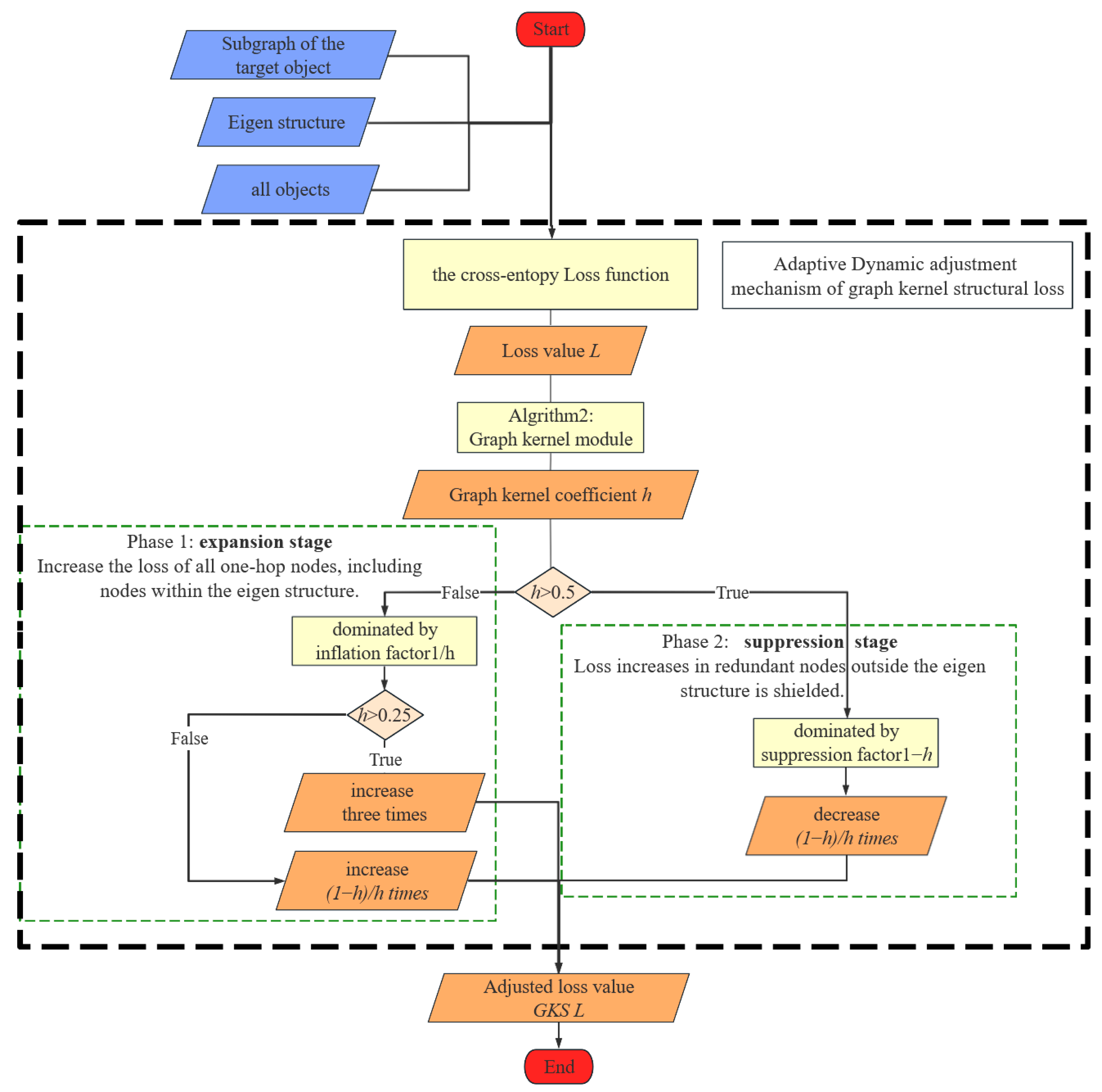
From Figure 4, we can observe that in the adaptive dynamic adjustment mechanism of GKS loss, two factors are introduced, namely, the suppression factor (1 − ) and the inflation factor (1/), for adaptively adjusting the tail structure loss. As depicted in the flowchart, the effect of the graph kernel coefficient derived from the eigenstructure mainly manifests in two aspects.
Firstly, in the expansion stage, when the graph kernel coefficient is less than 0.5, the inflation factor (1/) dominates, amplifying the contribution of to the total loss. Simultaneously, it also discriminates foreign objects of same spectra based on differences in the eigenstructure. This mechanism forces the model to focus more on learning the features of tail class objects and their environments during training, thereby improving the model’s performance in tail class recognition.
Subsequently, in the suppression stage, when the graph kernel coefficient exceeds the threshold of 0.5, the inflation factor begins to play a dominant role, suppressing the contribution of to the total loss, thus balancing the impact of one-hop redundant node errors caused by resampling on head classes. When tail class objects are accurately identified and their eigenstructures are isomorphic to the ground truth (GT), the specific loss term is forcibly zeroed out from the overall loss, aiming to reduce the potential impact of tail class errors on head class accuracy and, thus, improve overall recognition accuracy.
In summary, by combining the effects of the above two aspects, the eigenstructure not only acquires additional environmental structural information for tail class objects but also, after improving the accuracy of tail class objects, effectively balances the interference of redundant nodes in their environment through the introduction and regulation of the inflation and suppression factors. This enables our model to enhance the recognition performance of tail classes effectively while maintaining the recognition accuracy of head classes, thus achieving a more accurate and balanced classification outcome.
4. Results
This section details our experimental protocol and results. First, in Section 4.1, we provide a comprehensive overview of the dataset and details of the experimental implementation, with a focus on the target tail classes in the experimental. Next, Section 4.2 will explore the training loss of the experiment in depth, and conduct a detailed analysis on the loss of the target tail classes. Then, in Section 4.3, we will validate the effectiveness of the model by comparing its classification accuracy. Subsequently, in Section 4.4, we will further investigate the recognition performance of the target tail classes by comparing different depths of backbone networks. Finally, in Section 4.5, we will conduct a case-by-case analysis of individual samples.
4.1. Experiment Settings
In this subsection, we introduce the details related to the experiment. Firstly, we present the experimental dataset and its long-tailed effect analysis, validating the necessity of studying the dataset and discussing the tail classes that the experiment focuses on. Subsequently, we outline some implementation details of the experiment.
- (1)
- Dataset and long-tailed effect analysis
We collect remote sensing data from various regions such as oceans, coastal areas, and other types of areas using Google Earth to create an ocean dataset for this experiment. The obtained remote sensing images have a resolution of approximately 0.6 m and cover multiple regions including the East China Sea, South China Sea, East China region, Yangtze River Delta, and Pearl River Delta. The dataset consists of a total of 3601 images, each with a size of 224 × 224 pixels, and encompasses 30 different classes. The experimental dataset was randomly divided into training and validation sets in a ratio of approximately 8:2.
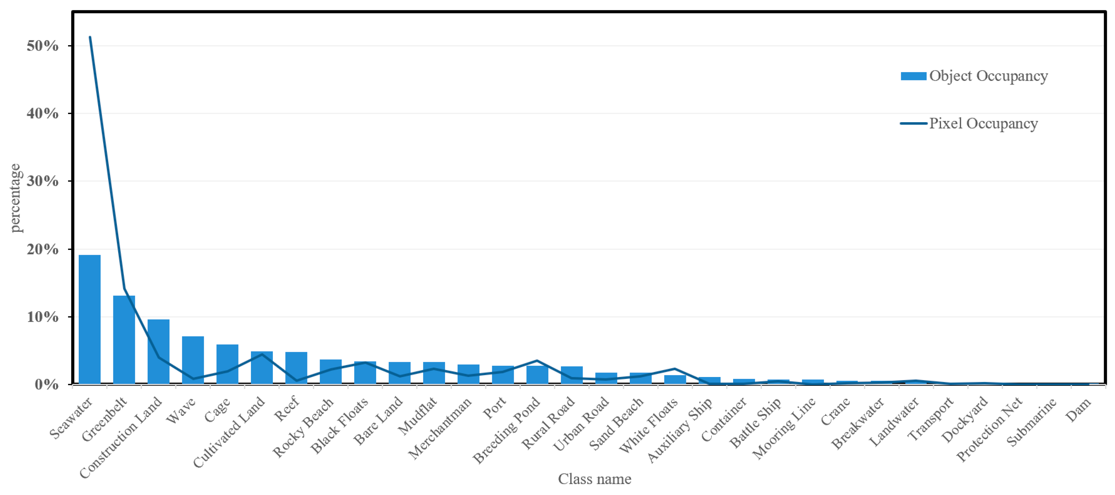
Due to the characteristic of the nearshore dataset, which predominantly consists of marine scenes, seawater is one of the main classes within the marine scene. As depicted in Figure 5, seawater accounts for the highest pixel occupancy among all classes, with a pixel area of approximately 90 million and its pixel occupancy reaching approximately 51.2%. In contrast, tail classes such as mooring line and protection net exhibit pixel occupancy all below 0.1%, with object occupancy in these classes measuring below 0.02%. This indicates an imbalance in the distribution of samples among classes in the dataset, where, apart from the samples in the head classes, the tail classes of samples are insufficient, with most samples concentrated in head classes. Therefore, it can be concluded that the experimental dataset belongs to a long-tailed distribution.
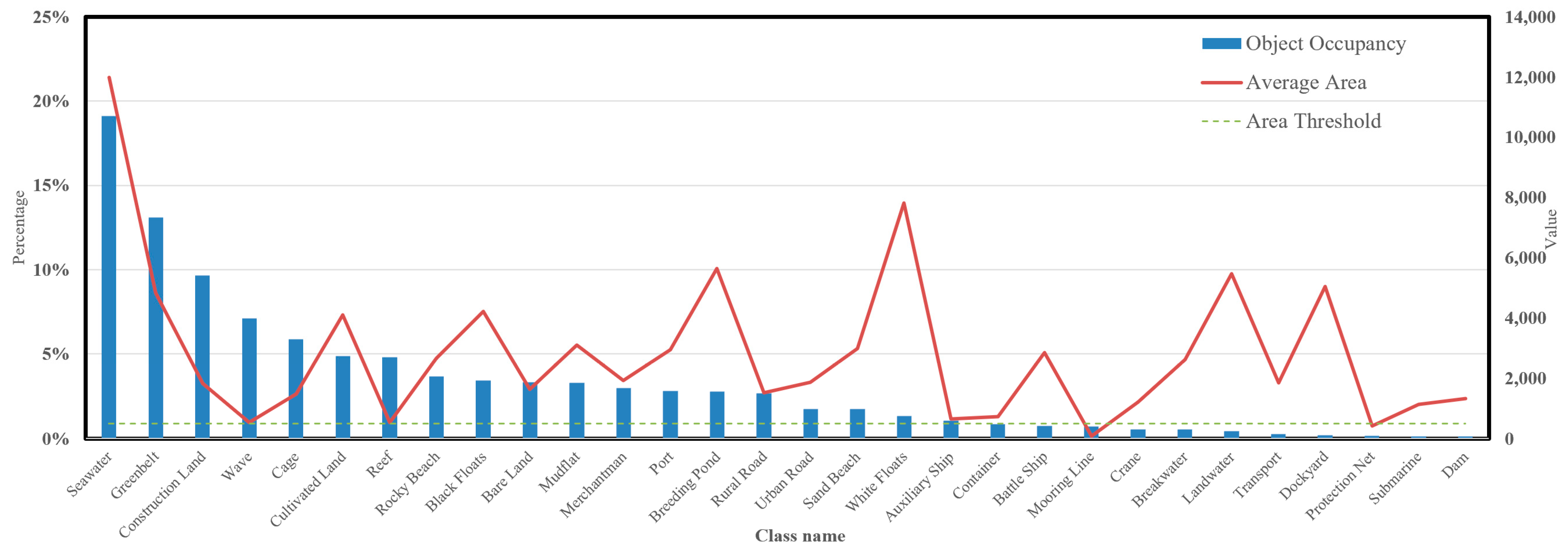
The features of small objects will be assimilated by the features of large objects after multiple layers of convolution. Figure 6 describes the distribution of object occupancy and the average object size for each class. Hence, this experiment mainly focuses on applying subsequent information enhancement to classes with a weak proportion of objects and small average object sizes. In this study, classes with object occupancy less than 1% and average object area less than 500 are selected as the target tail classes for this experiment: protection net and mooring line. The remaining classes are referred to as the head classes.
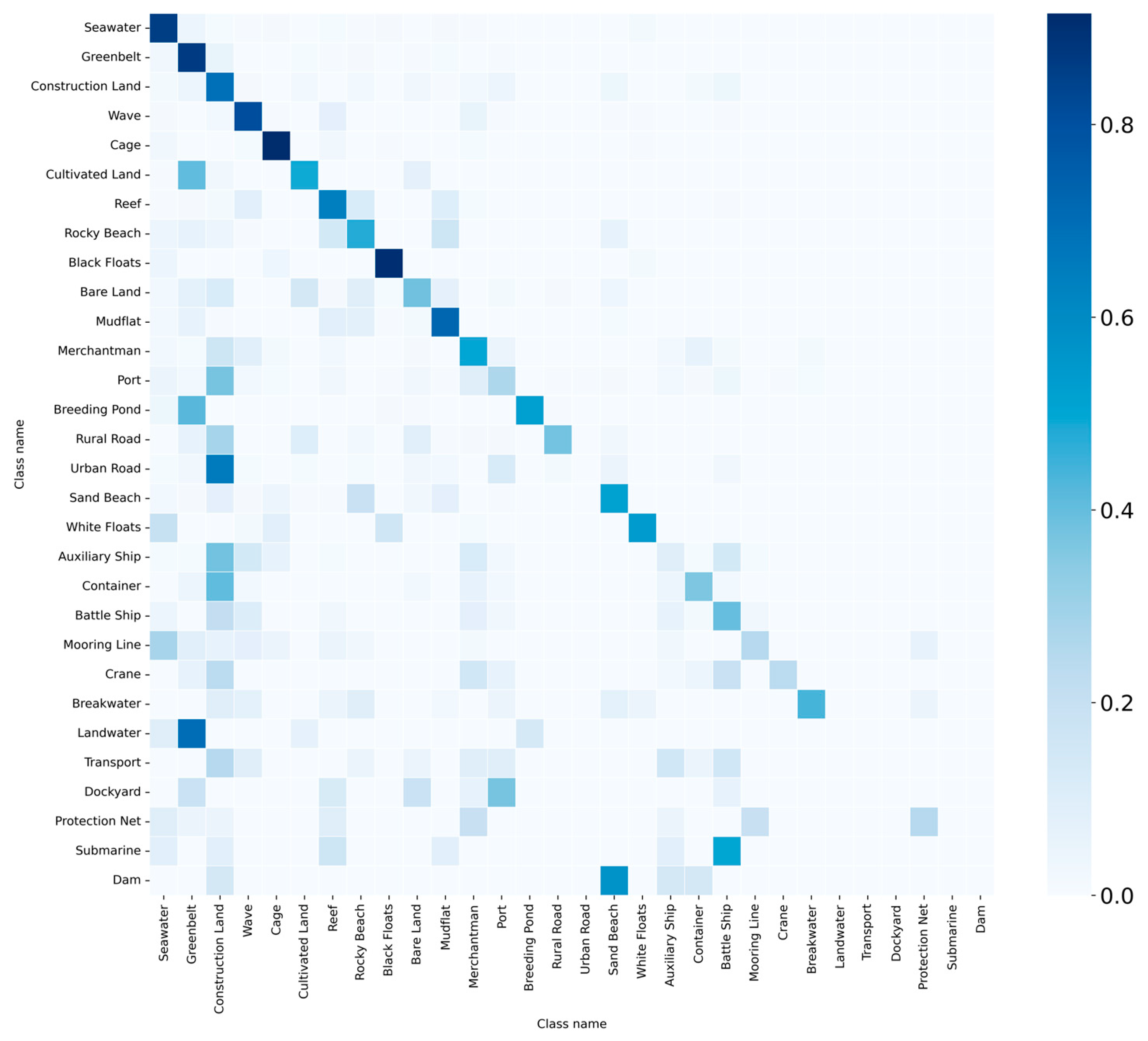
The long-tailed effect of the dataset has negative impact on the training and performance of deep learning models. Figure 7 shows the confusion matrix of the baseline model (GAT) on the validation set after training on this long-tailed dataset. From Figure 7, it can be observed that the precision of tail class objects is significantly lower than that of head class objects.
- (2)
- Implementation Details
During the model training phase, we empirically set the training epoch to 130, utilized the AdamW optimizer, and employed a batch size of 128 for training data. The learning rate strategy follows StepLR, which multiplies the learning rate by 0.8 every 20 epochs. All experiments were conducted in a consistent environment consisting of a 3090 GPU and an i9-10920X CPU.
4.2. Training Loss Analysis
This subsection mainly introduces the changes in the loss during the training process of the model.
4.2.1. Training Loss of the Baseline Model
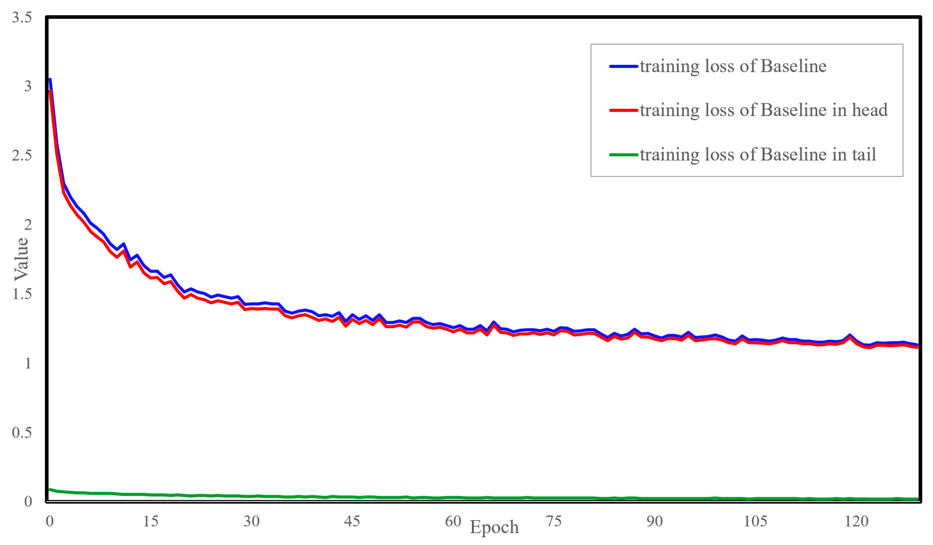
By displaying the variations in the loss, it reflects the progress and convergence performance of the model training. Figure 8 shows the variation curve of the loss function during the training phase of the baseline model.
In Figure 8, the blue curve represents the variation of the loss value of the baseline model. During the training process, the curves of the loss values for the target tail class (referred to as the tail classes hereafter) and the remaining classes (referred to as the head classes hereafter) are separately recorded, as shown by the green and red curves in the figure. It can be observed from the figure that the total loss curve of the baseline model rapidly decreases before 15 epochs and then gradually levels off until convergence. At the same time, compared by the red curve and green curve, it can be seen that the loss values for the target tail classes in the baseline model are very weak, with no significant downward trend in the loss values for the tail classes. This indirectly confirms that the tail classes in the long-tailed distribution are not receiving sufficient attention during model training. Therefore, it is necessary to enhance the information and weight of the tail classes.
4.2.2. Tail Loss Comparative Analysis of the Models
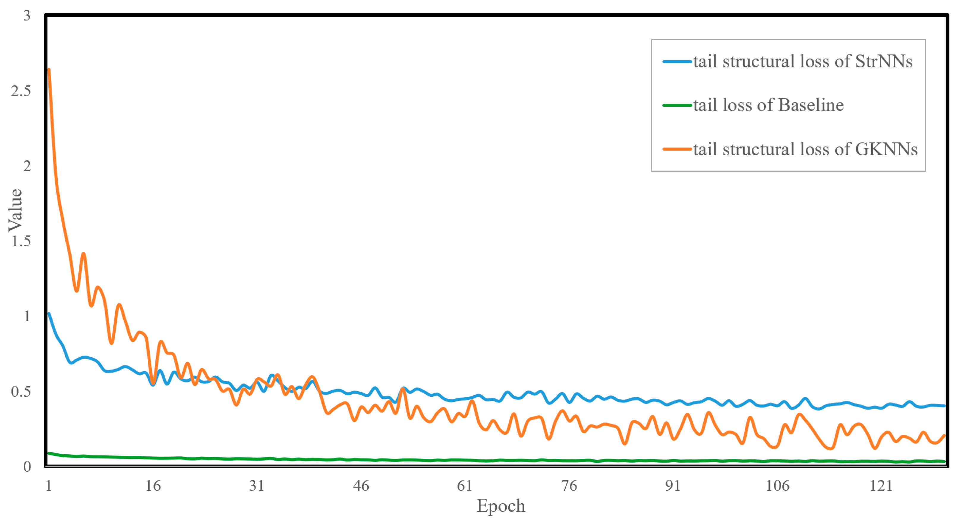
For the sake of facilitating subsequent comparative analysis of the models, the model trained by CBS loss is referred to as the StrNNs model, while the model trained by GKS loss is referred to as the GKNNs model. To assess the emphasis of different models on the target tail class, Figure 9 illustrates the variation of tail class loss with increasing training epochs for three models: the baseline model, the StrNNs model, and the GKNNs model.
The following conclusions can be drawn from Figure 9.
- Both the StrNNs model and the GKNNs model exhibit significant improvements in attention to tail classes. It can be observed from the figure that the tail loss curve of the baseline model consistently remains below the other two loss curves.
- Compared to the StrNNs model, the GKNNs model can achieve dynamic and adaptive adjustments of attention to tail classes. The tail structural loss value of the StrNNs model is initially around 1, while that of the GKNNs model, under the expansion effect of inflation factor, starts higher, at around 2.6. The tail structural loss curve of the GKNNs model experiences rapid descent initially, reaching parity with the StrNNs model around the 17th epoch. Subsequently, due to the dynamic suppression effect of the suppression factor, tail structural loss of the GKNNs model gradually decreases and becomes lower than that of the StrNNs model.
4.2.3. Training Loss of the GKNNs Model
The training process of the tail classes in the GKNNs model is further analyzed below to illustrate the adaptive dynamic adjustment capability of the tail structural loss.
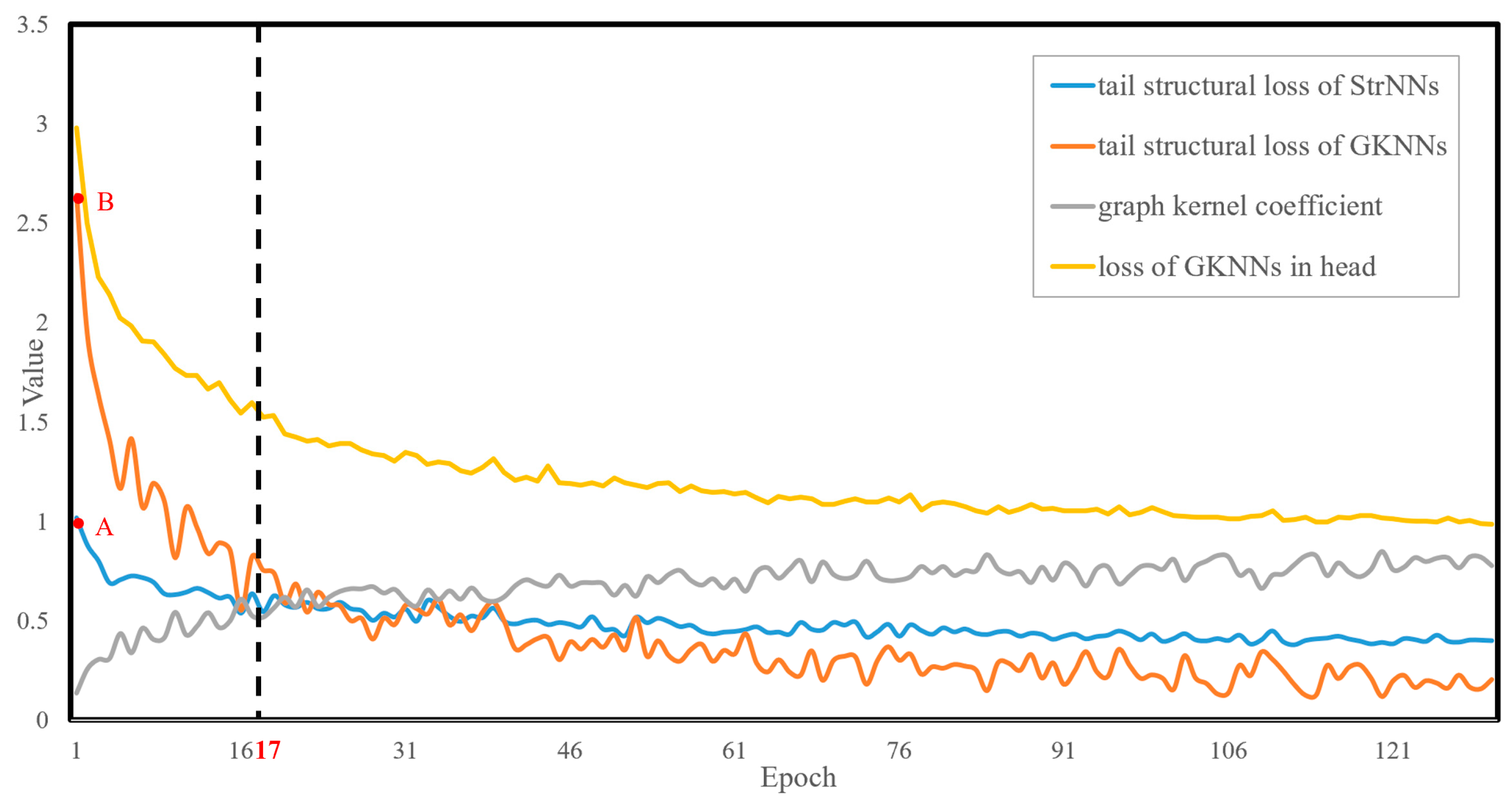
Figure 10 illustrates the tail structural loss curve of the GKNNs model under the influence of inflation and suppression factors, along with the tail loss curves of the StrNNs model and the head loss curves of GKNNs. Upon initial training, the model’s focus on the tail classes increases significantly due to the influence of the inflation factor, resulting in the tail structure loss for GKNNs being comparable to the loss of GKNNs in head classes. As training progresses, the tail structural loss of GKNNs decreases rapidly. Subsequently, to preserve the performance advantage of the head classes, the suppression factor becomes dominant, leading to a lower tail structure loss of GKNNs compared to StrNNs.
With the increase in training epochs, the training process can be divided into the following stages.
- Expansion stage: In the initial stages, the tail structural loss values of GKNNs and StrNNs are 2.6 (red point B in Figure 10) and 1.0 (red point A in Figure 10), while the loss of head classes is 2.9. By effect of the inflation factor, the initial tail structural loss is increased from 1.0 to 2.6, reaching the same order of magnitude as the head classes. This ensures that the tail class objects receive sufficient training. As the model continues to train, the graph kernel coefficient rapidly increases from 0 to 0.5, resulting in a simultaneous swift decline in the tail loss value of GKNNs. Around the 17th epoch, the graph kernel coefficient stabilizes around 0.5. Under the combined influence of the suppression and inflation factors, the tail structural loss value of GKNNs remains consistent with that of the StrNNs model.
- Suppression stage: After the 17th epoch, the graph kernel coefficient gradually approaches 1. Due to the dynamic suppression effect of the suppression factor, the tail structural loss of the GKNNs model gradually decrease and becomes lower than that of the StrNNs model for tail classes. Therefore, GKNNs can maintain the advantage of head classes without affecting the model’s focus on them.
4.3. Model Classification Precision Analysis
To demonstrate the object recognition performance of the model, the following arguments are provided from various semantic segmentation metrics.
- (1)
- Comparison of Overall Metrics
To quantitatively assess the performance of different models in semantic segmentation tasks, Table 1 presents the specific performance of GAT, StrNNs, and GKNNs on four evaluation metrics: overall object accuracy (OA (object)), overall pixel accuracy (OA (pixel)), kappa coefficient, and average object accuracy (AA (object)). GKNNs outperforms other models across all evaluation metrics, achieving an OA (object) of 68.82% and an impressive OA (pixel) of 86.02%. Compared to the baseline model (GAT), GKNNs shows improvements of 1.76% and 1.18% in OA (object) and OA (pixel), respectively. GKNNs also performs best in terms of kappa coefficient and AA (object), with values of 0.6567 and 47.85%, respectively, further confirming the reliability of GKNNs in semantic segmentation tasks. Although there is only a 1.76% improvement in OA(object), GKNNs shows a 6.16% increase in AA(object) over GAT. This indicates that GKNNs has a more balanced and stable classification performance across different classes, further demonstrating the effectiveness of GKPNN in addressing long-tail issues.
In contrast, StrNNs slightly underperforms compared to the baseline model, with decreases of 0.27% and 0.66% in OA (object) and OA (pixel), respectively. However, its AA (object) was 2.91% higher than that of GAT, indicating that StrNNs exhibits better average performance at the object level. This indirectly suggests that StrNNs effectively enhances the recognition performance of tail classes. Further explanations of the performance of each model will be provided subsequently.
- (2)
- Comparison of Class Object Accuracy
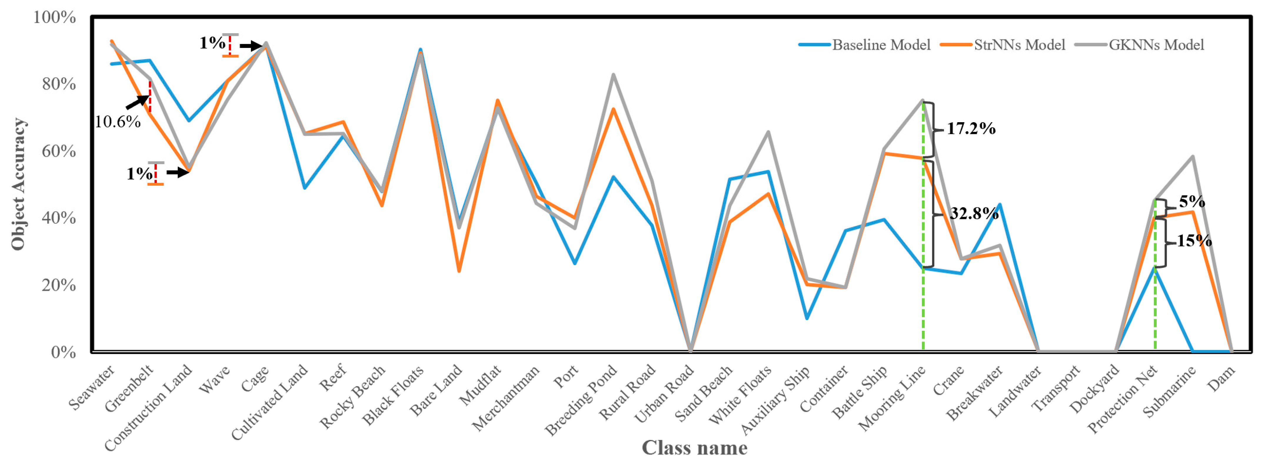
A comparative analysis of the semantic segmentation results of the proposed models is illustrated below, focusing on class perspectives. Figure 11 compares OA (object) of the three models for each class. Key observations about StrNNs include:
- Significant improvements of 32.8% and 15% are observed for the target tail classes, mooring line and protection net, respectively, compared to the baseline.
- As class 1 (seawater) is a crucial class in the eigenstructure of target tail classes, both StrNNs and GKNNs exhibit a 6% improvement in OA(object).
- However, excessive emphasis on target tail classes by StrNNs, aiming to balance training information between tail and head classes, slightly influences the recognition of some head classes (e.g., greenbelt, construction land, cage). Based on the situation above, an adaptive dynamic adjustment mechanism is introduced in GKNNs built upon StrNNs.
For GKNNs, the introduction of a graph kernel coefficient based on eigenstructure dynamically adjusts the weight of structural information enhancement for tail classes. This not only enhances tail classes’ structural information and model’s attention but also maintains head class performance, leading to a balanced class enhancement. Compared to StrNNs, the GKNNs model improves head class object accuracy (e.g., greenbelt, construction land, cage) by 10.6%, 1%, and 1%, respectively. Tail class accuracy also rises by 17.2% and 5%. The GKNNs model thus achieves balanced enhancement of overall classification performance while emphasizing tail class information.
The experimental results demonstrate that the proposed method significantly improves the recognition ability of minority and small target objects, thus achieving better performance when dealing with long-tailed datasets.
4.4. Backbone Model Analysis
To validate the performance of the backbone networks, we conducted a series of comparative experiments by replacing the backbone network in the GKNNs model. In GKNNs, the backbone network employs a residual block and a convolutional layer with stride of 2 from ResNet34, producing feature maps of size 112 × 112. Furthermore, we compare the differences in extraction performance of target tail class among ResNet34 models of different depths. Specifically, we further compare the performance of extracting feature maps of sizes 56 × 56 and 28 × 28 using ResNet34 at the output of the third and seventh residual blocks, respectively.
Based on the data in the Table 2, we can perform the following analysis.
Resnet34-112 × 112 achieves an object accuracy of 45.00% for the protection net, comparable to Resnet34-28 × 28 but lower than Resnet34-56 × 56’s 60.00%. However, for the mooring line, Res-net34-112 × 112 significantly outperforms the other versions, reaching 75.00%, compared to 37.50% for Resnet34-56 × 56 and 23.44% for Resnet34-28 × 28. Additionally, Resnet34-112 × 112 exhibits good performance in the average object accuracy of target tail classes, achieving 60.00%, surpassing Resnet34-56 × 56’s 48.75% and Resnet34-28 × 28’s 34.22%. In terms of object accuracy for all classes, all three versions of Resnet34 show similar performance, with Resnet34-112 × 112 and Resnet34-56 × 56 at 68.82% and 72.23%, respectively, and Resnet34-28 × 28 at 71.56%.
In terms of resource consumption comparison, regarding the number of parameters (Params), Resnet34-112 × 112 has 122,925 parameters, significantly lower than Resnet34-56 × 56 and Resnet34-28 × 28. For memory consumption (Memory(MB)), Resnet34-112 × 112 (ours) consumes 9002 MB, also lower than Resnet34-56×56 and Resnet34-28 × 28. In terms of time per iteration (time (second/iteration)), Resnet34-112 × 112 (ours) requires 18.16 s, less than Resnet34-56 × 56’s 22.44 s and Resnet34-28 × 28’s 22.93 s.
The experimental results indicate the following:
- The ResNet34-112 × 112 backbone architecture employed in GKNNs exhibits relatively good performance in identifying target tail classes.
- Regarding the effectiveness for target tail classes, particularly for the morning line class with the smallest average object area, it can be observed that deep networks are prone to confusing features of small objects, while feature maps from shallower networks demonstrate better recognition accuracy for tail classes [41].
- Considering both the extraction performance of target tail classes and the computational efficiency of the model, we opted for ResNet34-112 × 112 as the backbone network for GKNNs.
4.5. Instance Analysis
This subsection presents the adaptive dynamic adjustment mechanism of GKS loss and the semantic segmentation performance of GKNNs from the perspective of examples.
4.5.1. Analyzing Instances with the Structural Loss in Tail Classes
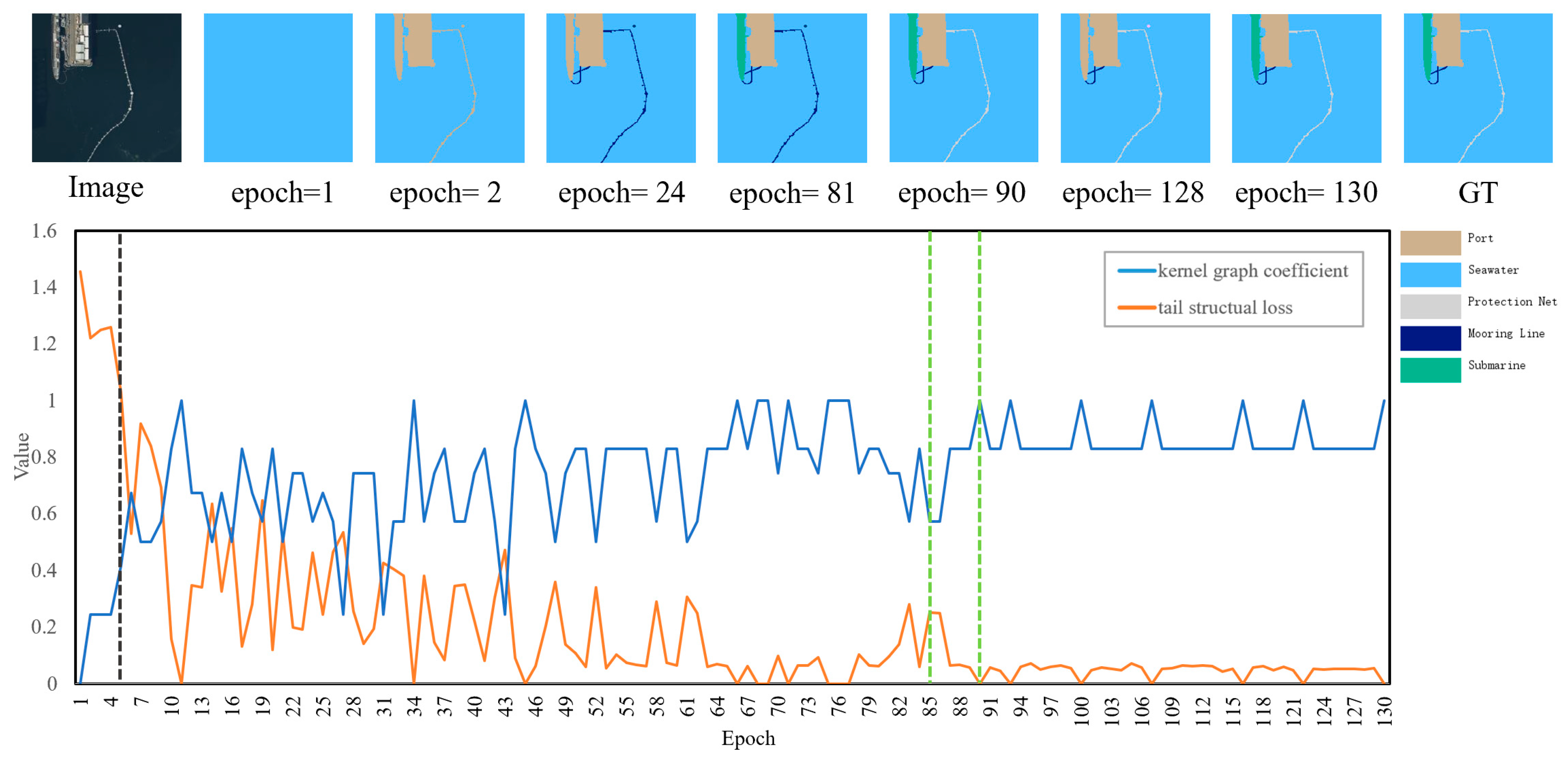
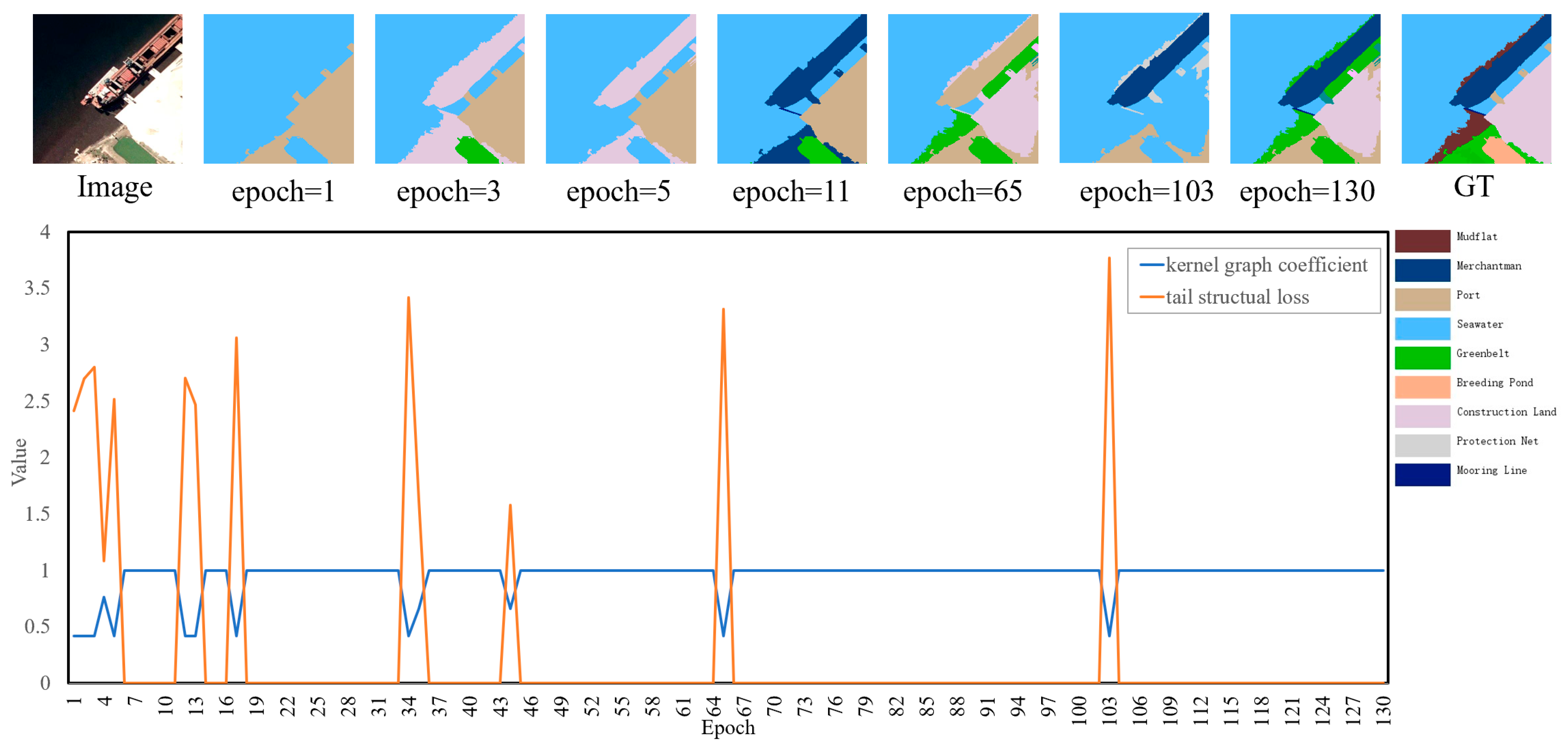
This subsection further analyzes and demonstrates the role of the graph kernel coefficient in adjusting the tail structural loss. Figure 12 and Figure 13 present the specific sample’s structural loss curve in each epoch in the archived models, along with the curve of the graph kernel coefficient of the tail target objects. It can be observed that the tail structural loss will adaptively adjust with the increase or decrease in the graph kernel coefficient.
In Sample 1, the central objects of the tail classes consist of one protection net object and two mooring line objects.
- Expansion stage: Before the fifth epoch, the graph kernel coefficient is less than 0.5, and the tail structural loss values of Sample 1 are magnified by the inflation factor. The tail structural loss decreases rapidly as the graph kernel coefficient increases.
- Suppression stage: After the fifth epoch, the graph kernel coefficient is greater than 0.5 and gradually approaches 1, and the tail structural loss enters a suppression stage. The kernel graph coefficient exhibits fluctuation during training, specifically dipping below 0.5 in epochs 27, 31, and 43.
- The local analysis of the adaptive dynamic adjustment mechanism: From the 85th epoch to the 90th epoch (as shown by green lines in Figure 12), it can be observed that when the eigenstructure objects of the tail classes are correctly predicted step by step, the graph kernel coefficient increases from 0.57 to 1 accordingly, and the corresponding tail structural loss decreases from 0.25 to 0. This causes the model to no longer pay more attention to the tail classes, thereby preserving the performance advantage of the head classes. By the 90th epoch, both mooring line and protection net objects, together with their respective eigenstructures, are correctly predicted and the graph kernel coefficient reaches 1, achieving adaptive dynamic adjustment of the tail structural loss.
Sample 2, identical to Sample 1, also follows the adaptive dynamic adjustment mechanism. In Sample 2, the central object of the tail class is the mooring line object. The prediction result for the 11th epoch accurately identifies the mooring line object and its neighboring nodes (e.g., merchantman and seawater) as they belong to the eigenstructure of mooring line. However, nodes outside this structure, such as construction land objects, are not correctly classified. Despite this, as they reside outside the mooring line’s eigenstructure, the graph kernel coefficient between the neighborhood subgraph and eigenstructure attains the value of 1, suppressing the tail structural loss associated with redundant nodes.
4.5.2. Analysis of Multiple Model Prediction Results for Typical Examples
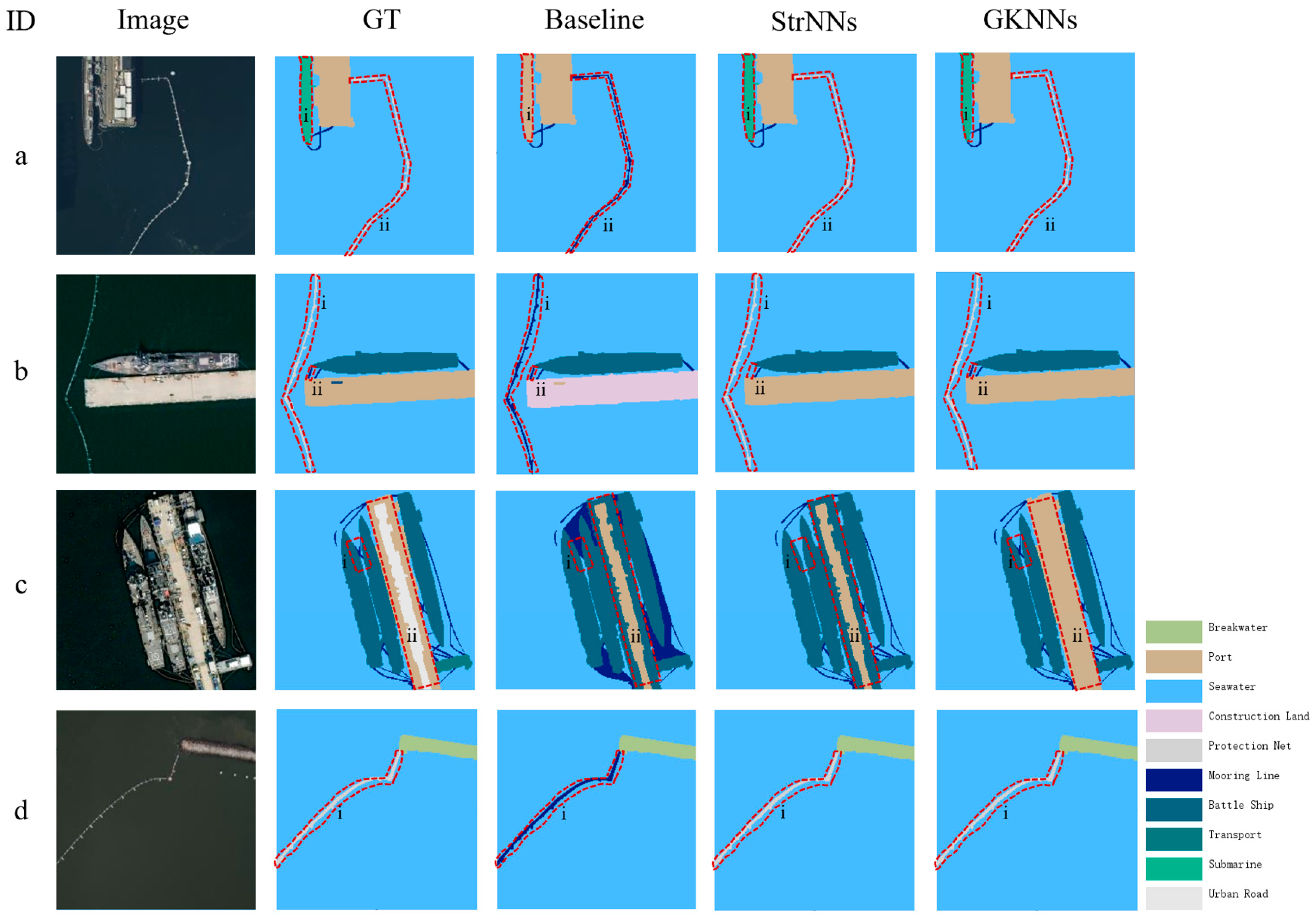
Figure 14 displays the prediction results of typical samples across multiple models to intuitively illustrate the effectiveness of GKNNs.
In Sample a, GKNNs accurately identifies submarines i, surpassing the baseline model. The baseline incorrectly classifies region ii objects as mooring line instead of protection net. Protection nets are typically directly adjacent to ports or independent within the ocean. By incorporating structural information, both StrNNs and GKNNs correctly identify the protection nets.
In Sample b, the baseline model erroneously identifies the protection net object i as a mooring line, while StrNNs and GKNNs correctly recognize it. Moreover, in this sample, we can observe that GKNNs exhibits better performance in mooring line identification compared to StrNNs.
In Sample c, StrNNs corrects baseline misidentifications of seawater objects i as mooring lines. GKNNs further improves the mooring line identification compared to StrNNs and achieves better recognition of port objects ii, which are crucial in the eigenstructure of mooring line.
In Sample d, the baseline model misidentifies a protection net i adjacent to breakwater (unlike mooring line) as a mooring line. Incorporating structural information rectifies the misidentification of this object, ensuring accurate protection net classification.
5. Discussion and Conclusions
To address the challenge of effectively recognizing tail classes, our research conducts the following work.
- This study introduces an effective mechanism for representing the structural features based on graph kernel principles to represent the structural features of tail classes and quantitatively describe the learning effectiveness of eigenstructure information. This mechanism leverages the eigenstructure information of tail class objects, in conjunction with basic visual features, to supplement and enhance the information of tail class objects, thereby partially compensate for the imbalance between tail and head class object information.
- Implemented with adaptive dynamic adjustment of the loss based on graph kernels, our designed inflation and suppression factors can dynamically control the strength of the enhancement information for tail classes. The results demonstrate that this mechanism ensures sufficient information for the recognition of tail classes while avoiding adverse impacts on the recognition of head classes.
- The experimental results show that the accuracy of target tail classes such as protection net and mooring line were improved by 20% and 50%, respectively, compared to the baseline model. Moreover, the average accuracy of object classes was increased by 6.16%. Experimental results demonstrate that the GKNNs model effectively addresses the recognition problem of minority and small targets, partially mitigates the phenomenon of foreign objects with similar spectra to tail objects, and improves its generalization ability and the semantic segmentation performance in remote sensing.
In the future, our work will focus on the following directions to further address the long-tail effect issue.
- The representation method for eigenstructure can be improved. In this research, the environmental information and eigenstructure of target tail classes objects are supplemented as background knowledge. The selection of eigenstructure depends on expert systems and simultaneously requires a certain amount of training samples. In the future, it is contemplated to use graph embedding models to better represent the eigenstructure, thereby enhancing the generalization of the model.
- More information of tail classes needs to be considered. Currently, the supplementary information for tail classes includes the visual and spatial features of target tail class objects. In subsequent work, more enriched attributes information such as the contours, areas, and the effect of corresponding geographical scene of tail classes can be embedded in the form of knowledge graph to supplement object information and balance the information gap between head and tail classes.
Author Contributions
W.C. supervised the study, designed the architecture, and revised the manuscript; Z.F. wrote the manuscript and designed the comparative experiments; X.X. made suggestions to the manuscript and assisted Z.F. in conducting the experiments; Y.T., J.C. and H.Z. made suggestions for the experiments and assisted in revising the manuscript; C.W. and Y.T. made datasets for the experiments. All authors have read and agreed to the published version of the manuscript.
Funding
This research was funded by the National Key R&D Program of China (Grant No. 2018YFC0810600, 2018YFC0810605) and National Natural Science Foundation of China (No. 42171415).
Data Availability Statement
The data presented in this study are available on request from the corresponding author due to the confidentiality requirements of the project.
Acknowledgments
The authors would like to thank the editors and the reviewers for their suggestions.
Conflicts of Interest
The authors declare no conflicts of interest.
References
- Yu, F.; Liu, Y.; Yumna, Z.; Gui, G.; Tao, M.; Qiang, S.; Jun, G. Long-tailed visual recognition with deep models: A methodological survey and evaluation. Neurocomputing 2022, 509, 290–309. [Google Scholar]
- Gupta, A.; Dollár, P.; Girshick, R. LVIS: A Dataset for Large Vocabulary Instance Segmentation. In Proceedings of the IEEE/CVF Conference on Computer Vision and Pattern Recognition, Long Beach, CA, USA, 15–20 June 2019; pp. 5351–5359. [Google Scholar]
- Wei, X. Image recognition of long-tail distribution: Pathways and progress. China Basic Sci. 2023, 25, 48–55. [Google Scholar]
- Buda, M.; Maki, A.; Mazurowski, M.A. A systematic study of the class imbalance problem in convolutional neural networks. Neural Netw. 2018, 106, 249–259. [Google Scholar] [CrossRef] [PubMed]
- Drummond, C.; Holte, R. C4.5, Class Imbalance, and Cost Sensitivity: Why Under-sampling Beats Oversampling. In Proceedings of the ICML Workshop on Learning from Imbalanced Data Sets, Washington, DC, USA, 21 August 2003; pp. 1–8. [Google Scholar]
- Chawla, N.V.; Bowyer, K.W.; Hall, L.O.; Philip Kegelmeyer, W. SMOTE: Synthetic minority over 2 sampling technique. J. Artif. Intell. Res. 2002, 16, 321–357. [Google Scholar] [CrossRef]
- Kang, B.; Xie, S.; Rohrbach, M.; Yan, Z.; Gordo, A.; Feng, J.; Kalantidis, Y. Decoupling representation and classifier for long-tailed recognition. In Proceedings of the International Conference on Learning Representations (ICLR), Addis Ababa, Ethiopia, 26–30 April 2020. [Google Scholar]
- He, H.; Bai, Y.; Garcia, E.; Li, S. Adaptive synthetic sampling approach for imbalanced learning. In Proceedings of the IEEE International Joint Conference on Neural Networks (IEEE World Congress on Computational Intelligence), Hong Kong, China, 1–8 June 2008. [Google Scholar]
- Mahajan, D.; Girshick, R.; Ramanathan, V.; He, K.; Paluri, M.; Li, Y.; Bharambe, A.; Van Der Maaten, L. Exploring the limits of weakly supervised pretraining. In Proceedings of the European Conference on Computer Vision (ECCV), Munich, Germany, 8–14 September 2018; pp. 181–196. [Google Scholar]
- Lin, T.Y.; Goyal, P.; Girshick, R.; He, K.; Dollar, P. Focal loss for dense object detection. In Proceedings of the IEEE International Conference on Computer Vision, Venice, Italy, 22–29 October 2017; pp. 2980–2988. [Google Scholar]
- Cui, Y.; Jia, M.; Lin, T.Y.; Song, Y.; Belongie, S. Class-balanced loss based on effective number of samples. In Proceedings of the IEEE/CVF Conference on Computer Vision and Pattern Recognition, Long Beach, CA, USA, 15–20 June 2019; pp. 9268–9277. [Google Scholar]
- Wang, Y.; Ramanan, D.; Hebert, M. Learning to model the tail. In Proceedings of the 31st Conference on Neural Information Processing Systems, Long Beach, CA, USA, 4–9 December 2017. [Google Scholar]
- Liu, B.; Li, H.; Kang, H.; Hua, G.; Vasconcelos, N. GistNet: A geometric structure transfer network for long-tailed recognition. In Proceedings of the IEEE/CVF International Conference on Computer Vision (ICCV), Montreal, QC, Canada, 10–17 October 2021; pp. 8209–8218. [Google Scholar]
- Zhang, Y.; Cheng, D.Z.; Yao, T.; Yi, X.; Hong, L.; Chi, E.H. A model of two tales: Dual transfer learning framework for improved long-tail item recommendation. In Proceedings of the Web Conference 2021, Ljubljana, Slovenia, 19–23 April 2021; pp. 2220–2231. [Google Scholar]
- Cui, Y.; Song, Y.; Sun, C.; Howard, A.; Belongie, S. Large scale fine-grained categorization and domain-specific transfer learning. In Proceedings of the IEEE conference on computer vision and pattern recognition, Salt Lake City, UT, USA, 18–23 June 2018; pp. 4109–4118. [Google Scholar]
- Hu, X.; Jiang, Y.; Tang, K.; Chen, J.; Miao, C.; Zhang, H. Learning to segment the tail. In Proceedings of the IEEE/CVF Conference on Computer Vision and Pattern Recognition, Seattle, WA, USA, 13–19 June 2020; pp. 14045–14054. [Google Scholar]
- Liu, J.; Sun, Y.; Han, C.; Dou, Z.; Li, W. Deep representation learning on long-tailed data: A learnable embedding augmentation perspective. In Proceedings of the IEEE/CVF Conference on Computer Vision and Pattern Recognition, Seattle, WA, USA, 13–19 June 2020; pp. 2970–2979. [Google Scholar]
- Taha, A.Y.; Tiun, S.; Abd Rahman, A.H.; Sabah, A. Multilabel Over-Sampling and under-Sampling with Class Alignment for Imbalanced Multilabel Text Classification. J. Inf. Commun. Technol. 2021, 20, 423–456. [Google Scholar] [CrossRef]
- Zhou, B.; Cui, Q.; Wei, X.S.; Chen, Z.M. BBN: Bilateral-branch network with cumulative learning for long-tailed visual recognition. In Proceedings of the IEEE/CVF Conference on Computer Vision and Pattern Recognition, Seattle, WA, USA, 13–19 June 2020; pp. 9719–9728. [Google Scholar]
- Cao, K.; Wei, C.; Gaidon, A.; Aréchiga, N.; Ma, T. Learning imbalanced datasets with label-distribution-aware margin loss. In Proceedings of the Neural Information Processing Systems (NeurIPS), Vancouver, BC, Canada, 8–14 December 2019. [Google Scholar]
- Cui, W.; He, X.; Yao, M.; Wang, Z.; Hao, Y.; Li, J.; Wu, W.; Zhao, H.; Xia, C.; Li, J. Knowledge and Spatial Pyramid Distance-Based Gated Graph Attention Network for Remote Sensing Semantic Segmentation. Remote Sens. 2021, 13, 1312. [Google Scholar] [CrossRef]
- Cui, W.; Hao, Y.; Xu, X.; Feng, Z.; Zhao, H.; Xia, C.; Wang, J. Remote Sensing Scene Graph and Knowledge Graph Matching with Parallel Walking Algorithm. Remote Sens. 2022, 14, 4872. [Google Scholar] [CrossRef]
- Zhong, Z.; Cui, J.; Liu, S.; Jia, J. Improving calibration for long-tailed recognition. In Proceedings of the IEEE/CVF Conference on Computer Vision and Pattern Recognition (CVPR), Nashville, TN, USA, 20–25 June 2021; pp. 16489–16498. [Google Scholar]
- Han, H.; Wang, W.Y.; Mao, B.H. Borderline-SMOTE: A New Over-Sampling Method in Imbalanced Data Sets Learning. In Proceedings of the International Conference on Advances in Intelligent Computing, Hefei, China, 23–26 August 2005; pp. 878–887. [Google Scholar]
- Chang, N.; Yu, Z.; Wang, Y.X.; Anandkumar, A.; Fidler, S.; Alvarez, J.M. Image-Level or Object-Level? A Tale of Two Resampling Strategies for Long-Tailed Detection. In Proceedings of the International Conference on Machine Learning, Vienna, Austria, 18–24 July 2021; pp. 1463–1472. [Google Scholar]
- Wei, H.; Tao, L.; Xie, R.; Feng, L.; An, B. Open-Sampling: Exploring out-of-Distribution Data for Re-Balancing Long-Tailed Datasets. In Proceedings of the International Conference on Machine Learning, Baltimore, MD, USA, 17–23 July 2022; pp. 23615–23630. [Google Scholar]
- Yu, H.; Du, Y.; Wu, J. Reviving Undersampling for Long-Tailed Learning. Available online: https://arxiv.org/abs/2401.16811 (accessed on 30 January 2024).
- Wei, F.; Stolfo, J.S.; Zhang, J.; Chan, P.K. AdaCost: Misclassification cost- sensitive boosting. In Proceedings of the 16th International Conference on Machine Learning, SanMateo, USA, 27–30 June 1999. [Google Scholar]
- Khan, S.H.; Hayat, M.; Bennamoun, M.; Sohel, F.A.; Togneri, R. Cost-Sensitive Learning of Deep Feature Representations from Imbalanced Data. IEEE Trans. Neural Netw. Learn. Syst. 2017, 29, 3573–3587. [Google Scholar] [PubMed]
- Fernando, K.R.M.; Tsokos, C.P. Dynamically Weighted Balanced Loss: Class Imbalanced Learning and Confidence Calibration of Deep Neural Networks. IEEE Trans. Neural Netw. Learn. Syst. 2021, 33, 2940–2951. [Google Scholar] [CrossRef] [PubMed]
- Dong, Q.; Gong, S.; Zhu, X. Class Rectification Hard Mining for Imbalanced Deep Learning. In Proceedings of the IEEE International Conference on Computer Vision, Venice, Italy, 22–29 October 2017; pp. 1851–1860. [Google Scholar]
- Xiang, L.; Ding, G.; Han, J. Learning from multiple experts: Self-paced knowledge distillation for long-tailed classification. In Proceedings of the Computer Vision–ECCV 2020: 16th European Conference, Glasgow, UK, 23–28 August 2020; pp. 247–263. [Google Scholar]
- Haussler, D. Convolution Kernels on Discrete Structures; UCS-CRL-99-10; University of California at Santa Cruz: Santa Cruz, CA, USA, 1999. [Google Scholar]
- Gärtner, T. A survey of kernels for structured data. ACM SIGKDD Explor. Newsl. 2003, 5, 49–58. [Google Scholar] [CrossRef]
- Gärtner, T.; Flach, P.; Wrobel, S. On graph kernels: Hardness results and efficient alternatives. Learn. Theory Kernel Mach. 2013, 2777, 129–143. [Google Scholar]
- Shervashidze, N.; Vishwanathan, S.V.N.; Petri, T.; Mehlhorn, K.; Borgwardt, K. Efficient graphlet kernels for large graph comparison. In Proceedings of the 22nd International Conference on Artificial Intelligence and Statistics, Naha, Okinawa, Japan, 16–18 April 2009; pp. 488–495. [Google Scholar]
- Shervashidze, N.; Schweitzer, P.; Leeuwen, E.J.V.; Mehlhorn, K.; Borgwardt, K.M. Weisfeiler-lehman graph kernels. J. Mach. Learn. Res. 2011, 12, 2539–2561. [Google Scholar]
- Nikolentzos, G.; Meladianos, P.; Tixier, A.J.P.; Skianis, K.; Vazirgiannis, M. Kernel graph convolutional neural networks. In Proceedings of the 27th International Conference on Artificial Neural Networks, Rhodes, Greece, 4–7 October 2018; pp. 22–32. [Google Scholar]
- Du, S.S.; Hou, K.; Póczos, B.; Salakhutdinov, R.; Wang, R.; Xu, K. Graph neural tangent kernel: Fusing graph neural networks with graph kernels. In Proceedings of the Neural Information Processing Systems (NeurIPS), Vancouver, BC, Canada, 8–14 December 2019. [Google Scholar]
- Feng, A.; You, C.; Wang, S.; Tassiulas, L. KerGNNs: Interpretable graph neural networks with graph kernels. In Proceedings of the AAAI Conference on Artificial Intelligence, Vancouver, Canada, 22–28 February 2022; pp. 6614–6622. [Google Scholar]
- Luo, W.; Li, Y.; Urtasun, R.; Zemel, R. Understanding the effective receptive field in deep convolutional neural networks. In Proceedings of the 30th Conference on Neural Information Processing Systems (NIPS 2016), Barcelona, Spain, 5–10 December 2016. [Google Scholar]
Figure 1.
Schematic diagram of a long-tailed distribution dataset. This figure depicts the overall proportion of objects for each class in the experimental dataset.
Figure 1.
Schematic diagram of a long-tailed distribution dataset. This figure depicts the overall proportion of objects for each class in the experimental dataset.

Figure 2.
Overall network architecture of the GKNNs model.

Figure 3.
Dynamic adjustment curve varying with h. The red segment indicates the expansion stage, while the blue segment indicates the suppression stage.
Figure 3.
Dynamic adjustment curve varying with h. The red segment indicates the expansion stage, while the blue segment indicates the suppression stage.

Figure 4.
Flowchart of the adaptive dynamic adjustment mechanism of GKS loss, divided into expansion stage and suppression stage.
Figure 4.
Flowchart of the adaptive dynamic adjustment mechanism of GKS loss, divided into expansion stage and suppression stage.

Figure 5.
Distribution of the proportion of objects and pixels for each class in the entire dataset. The bar chart represents the proportion of objects, while the blue line indicates the proportion of pixels.
Figure 5.
Distribution of the proportion of objects and pixels for each class in the entire dataset. The bar chart represents the proportion of objects, while the blue line indicates the proportion of pixels.

Figure 6.
Comparison of the proportion and average area of objects for each class. The tail classes with fewer objects and smaller areas are the protection net and mooring line. Subsequent experiments target these two tail classes for resolution.
Figure 6.
Comparison of the proportion and average area of objects for each class. The tail classes with fewer objects and smaller areas are the protection net and mooring line. Subsequent experiments target these two tail classes for resolution.

Figure 7.
Confusion matrix of the baseline model. The confusion matrix presents the names of classes along both its horizontal and vertical axes. To enhance the graphical representation, the number of objects belonging to each class is normalized.
Figure 7.
Confusion matrix of the baseline model. The confusion matrix presents the names of classes along both its horizontal and vertical axes. To enhance the graphical representation, the number of objects belonging to each class is normalized.

Figure 8.
Loss curve plot during training phase of the baseline model. The horizontal axis represents epochs, while the vertical axis denotes the loss value.
Figure 8.
Loss curve plot during training phase of the baseline model. The horizontal axis represents epochs, while the vertical axis denotes the loss value.

Figure 9.
Loss curves obtained by each model for the target tail class during training. The green, blue, and orange curves represent the changes in tail class loss values for the baseline model, the StrNNs model, and the GKNNs model, respectively.
Figure 9.
Loss curves obtained by each model for the target tail class during training. The green, blue, and orange curves represent the changes in tail class loss values for the baseline model, the StrNNs model, and the GKNNs model, respectively.

Figure 10.
Analysis of the training loss curve for the tail structural loss of the GKNNs model. The blue curve represents the tail structural loss curve of the StrNNs model, while the orange and gray curves depict the tail structural loss curve of GKNNs and the variation of graph kernel coefficient h with increasing training epochs, respectively.

Figure 11.
Comparison of object accuracy for each class among the three models. The horizontal axis represents the class, and the vertical axis represents the object accuracy.
Figure 11.
Comparison of object accuracy for each class among the three models. The horizontal axis represents the class, and the vertical axis represents the object accuracy.

Figure 12.
The tail structural loss curve and the graph kernel coefficient curve for Sample 1 at each epoch, along with prediction plots for key epochs.
Figure 12.
The tail structural loss curve and the graph kernel coefficient curve for Sample 1 at each epoch, along with prediction plots for key epochs.

Figure 13.
The tail structural loss curve and the graph kernel coefficient curve for Sample 2 at each epoch, along with prediction plots for key epochs.
Figure 13.
The tail structural loss curve and the graph kernel coefficient curve for Sample 2 at each epoch, along with prediction plots for key epochs.

Figure 14.
Comparison of predicted results from different models for typical samples; (a–d) represent four different typical samples.
Figure 14.
Comparison of predicted results from different models for typical samples; (a–d) represent four different typical samples.


Table 1.
Comparison of overall metrics of the models.
| Model | OA (Object) | OA (Pixel) | Kappa | AA (Object) |
|---|---|---|---|---|
| GAT | 67.06% | 84.84% | 0.6366 | 41.69% |
| StrNNs | 66.89% | 84.18% | 0.6364 | 44.60% |
| GKNNs | 68.82% | 86.02% | 0.6567 | 47.85% |
Table 2.
Comparison of backbone model performance.
| Resnet34-112 × 112 (Ours) | Resnet34-56 × 56 | Resnet34-28 × 28 | |
|---|---|---|---|
| Protection net OA(object) | 45.00% | 60.00% | 45.00% |
| Mooring line OA(object) | 75.00% | 37.50% | 23.44% |
| AA(object) of target tail classes | 60.00% | 48.75% | 34.22% |
| OA(object) of all classes | 68.82% | 72.23% | 71.56% |
| Params | 122,925 | 344,877 | 1,460,293 |
| Memory(MB) | 9002 | 9704 | 9776 |
| Time (second/iteration) | 18.16 | 22.44 | 22.93 |
Disclaimer/Publisher’s Note: The statements, opinions and data contained in all publications are solely those of the individual author(s) and contributor(s) and not of MDPI and/or the editor(s). MDPI and/or the editor(s) disclaim responsibility for any injury to people or property resulting from any ideas, methods, instructions or products referred to in the content. |
© 2024 by the authors. Licensee MDPI, Basel, Switzerland. This article is an open access article distributed under the terms and conditions of the Creative Commons Attribution (CC BY) license (https://creativecommons.org/licenses/by/4.0/).
Share and Cite
MDPI and ACS Style
Cui, W.; Feng, Z.; Chen, J.; Xu, X.; Tian, Y.; Zhao, H.; Wang, C. Long-Tailed Effect Study in Remote Sensing Semantic Segmentation Based on Graph Kernel Principles. Remote Sens. 2024, 16, 1398. https://doi.org/10.3390/rs16081398
AMA Style
Cui W, Feng Z, Chen J, Xu X, Tian Y, Zhao H, Wang C. Long-Tailed Effect Study in Remote Sensing Semantic Segmentation Based on Graph Kernel Principles. Remote Sensing. 2024; 16(8):1398. https://doi.org/10.3390/rs16081398
Chicago/Turabian StyleCui, Wei, Zhanyun Feng, Jiale Chen, Xing Xu, Yueling Tian, Huilin Zhao, and Chenglei Wang. 2024. "Long-Tailed Effect Study in Remote Sensing Semantic Segmentation Based on Graph Kernel Principles" Remote Sensing 16, no. 8: 1398. https://doi.org/10.3390/rs16081398
Note that from the first issue of 2016, this journal uses article numbers instead of page numbers. See further details here.