Enhancing Soil Moisture Active–Passive Estimates with Soil Moisture Active–Passive Reflectometer Data Using Graph Signal Processing

Abstract

The Soil Moisture Active–Passive (SMAP) mission has greatly contributed to the use of remote sensing technologies for monitoring the Earth’s land surface and estimating geophysical parameters that influence the climate system. Since the SMAP mission switched its radar receiver to allow the reception of Global Positioning System (GPS) signals, Global Navigation Satellite System Reflectometry (GNSS-R) configuration has been enabled, providing full polarimetric forward scattering measurements of the Earth’s surface, also known as SMAP Reflectometry or SMAP-R. Polarimetric GNSS-R is beneficial for sensing land surface properties, especially for more accurate estimations of soil moisture (SM) in densely vegetated areas. In this study, we explore the opportunity to enhance SMAP mission soil moisture estimates using reflected GNSS signals. We achieve this by interpolating the sparse reflectivity data with terrain information to disaggregate radiometer brightness temperatures. Our main objective is to present a novel algorithm based on Graph Signal Processing (GSP) that uses reflectometry data to enhance SMAP radiometer observations and ultimately improve SM retrievals. By implementing methods from the GSP field, we formulate the reflectivity interpolation problem as a signal reconstruction on a graph, where the weights of the edges between the nodes are chosen as a function of geophysical information. Subsequently, using the retrieved reflectivity maps, we increase the resolution of the brightness temperature data, leading to an improvement in the SM estimates. Initial findings indicate that our GSP method presents a promising alternative for analyzing sparse remote sensing observations, leveraging Earth’s surface geophysical information. This approach results in a notable improvement, with a reduced Root Mean Square Error (RMSE) of 11.8% compared to SMAP data and a reduction in unbiased RMSE (uRMSE) by 14.7% over vegetated areas.

1. Introduction

The advancement of remote sensing technologies has been instrumental in enriching our comprehension of Earth’s processes, particularly in analyzing Earth’s hydrological and climatic phenomena. These technologies, including radiometers, synthetic aperture radars (SAR), and optical sensors, supply diverse and valuable data that open new research avenues. These advancements enrich remote sensing applications that enhance crop yield prediction, facilitate the detection of vegetation changes, improve weather forecasting, and contribute to the analysis of the global carbon cycle. To accurately model hydrologic processes, it is vital to consider Essential Climate Variables (ECVs) such as soil moisture (SM), precipitation, and evapotranspiration [1]. ECVs are physical, chemical, or biological variables that play a critical role in characterizing Earth’s climate and serve as key indicators of environmental changes, making their effective monitoring essential for ecosystem analysis. In particular, SM, a biological and geophysical indicator, plays a key role in the Earth’s system, influencing vital processes like vegetation growth, climate predictions, and hydrological models [2]. It directly affects plant health, growth, and water availability for vegetation. Acting as a crucial land geophysical metric, SM mediates the exchange of energy and water between the land’s surface and the atmosphere. Therefore, the precision and comprehension of SM metrics are indispensable for climate prediction, water resource management, and the refinement of hydrological models. As a necessary gauge of terrestrial moisture conditions, SM aids in drought monitoring [3], vegetation development [4], and water conservation [5]. Instruments such as radars, radiometers, and reflectometers are typically used for SM measurements, given that microwave frequencies resonate with variations in soil dielectric properties due to moisture content [6]. Among the options, L-band frequencies are preferred due to their providing resilience against atmospheric losses and vegetation cover interferences. Integrating data from various instruments aimed at enhancing L-band measurements offers significant improvements in Soil Moisture (SM) accuracy and, alternatively, enhances spatial and temporal resolutions. An example of this approach is demonstrated in the SMAP (Soil Moisture Active–Passive) mission, designed to combine passive and active remote sensing technologies, an L-band radiometer, and an L-band radar.

The primary objective of merging data in this context is to enhance the spatial resolution of SM estimates. The SMAP radiometer, while offering accurate SM estimations, is limited by a spatial resolution of 36 km. In contrast, the radar component of SMAP provided a much finer spatial resolution, capable of reaching up to 3 km. By combining these datasets, it was possible to produce a downscaled SM product with an improved resolution of 9 km. This approach leveraged the strengths of both the radiometer and the radar, leading to a substantial enhancement in the overall quality of the data [7]. However, shortly after its launch, the SMAP radar transmitter experienced an anomaly and stopped collecting data [8]. As a result, the official SMAP product relied primarily on the brightness temperatures ($T_b$) measured by the L-band microwave radiometer to compute SM maps [7] and freeze/thaw (F/T) state maps on a fixed 36 km EASE-Grid 2.0. As a novel effort, after the radar transmitter malfunctioned, SMAP Reflectometry (SMAP-R) emerged as an opportunistic polarimetric GNSS-R instrument. SMAP radar receiver bandpass frequency filter was modified to be centered at 1227.42 MHz to receive in bistatic configuration the Global Positioning System (GPS) L2C signals. SMAP-R has specific advantages compared to traditional GNSS-R missions due to its high-gain antenna, which provides high SNR for low integration times, and the linear polarimetric antenna, which enables the hybrid compact polarimetric (HCP) capability [9]. On the other hand, the main drawback of SMAP-R comes from the highly directive scanning antenna as well, which significantly reduces the number of measurements per day that the instrument provides. A polarimetric GNSS-R instrument in HCP configuration allows computation of the full Stokes parameters describing a polarimetric portrait of the surface under observation [10].

In vegetated areas, the phenomenon of dispersive reflection, which affects the signals received by radiometric sensors, leads to a signal polarization signature. This polarization signature allows SMAP-R to discriminate details about the physical properties of vegetation, the texture, roughness, and SM levels [11]. In general, over soil surfaces, the characteristics of the GNSS-R reflection mostly depend on SM and are additionally affected by surface roughness and vegetation. The methodology for formulating the Stokes parameters and their calibration is detailed in [12,13]. The surface effects on the GNSS-R signals have been assessed using the Stokes parameters for the SMAP-R dataset [14]. The analysis of SMAP-R data combined with SMAP radiometer data has shown efficacy in the estimation of SM maps by improving the spatial resolution while maintaining and checking the unbiased SM estimation error [14]. The results of this data merging strategy suggest the potential for combining sparse datasets from GNSS-R with coarser radiometric data to achieve more accurate and detailed SM assessments.

Developing a data processing methodology that not only accounts for the nonlinear relationships among land geophysical parameters and measurements but also addresses the fact that the datasets have differing spatial resolutions would be highly advantageous for SM retrievals. In this context, there has been a growing focus on the development of SM retrieval algorithms that effectively incorporate terrain data. For example, in [15,16], the authors introduced the trilinear regression-based reflectivity–vegetation–roughness algorithm. This algorithm derives SM estimations at a 36 km resolution by considering Cyclone Global Navigation Satellite System (CYGNSS) [15] reflectivity, along with the SMAP vegetation opacity and roughness coefficient. However, this algorithm has limitations in terms of the number of geophysical variables it considers. In [17], the authors developed a time-series approach for SM retrieval, using maximum and minimum SM values from SMAP to establish the system’s limits. As a key point, the changes in vegetation and surface roughness evolve significantly more slowly than changes in SM. In [2], the authors presented a fully connected Artificial Neural Network (ANN) to account for the effects of vegetation and ground dynamics on SM estimation. Although they used in situ SM measurements from International SM Network (ISMN) sites as reference labels, most of these sites were located on relatively non-mountainous surfaces with low-to-moderate vegetation cover, such as croplands, grasslands, and savannas. This limits the analysis’s ability to capture scattering effects, considering the significant temporal and spatial variation and non-uniformity of vegetation parameters.

Addressing the challenge of integrating diverse datasets for SM estimation, this manuscript introduces an innovative graph-based data integration technique for SM enhancement using the SMAP-R dataset and terrain characteristics. Our approach is based on Graph Signal Processing (GSP), which is well-suited for processing signals that are in irregular domains and result from physical processes influenced by multiple variables. Graph models efficiently capture the structural information of images, and their application in image processing has been proven effective in numerous applications [18]. Recently, graph-based methods have been explored in remote sensing applications. For example, Change Detection (CD) algorithms have used the Nystrom extension to represent images as graphs, minimizing similarities among them to detect changes [19]. Path-wise graphs [20] and super pixel-wise graphs [21], based on the self-similarity property, have been constructed to capture image structures and calculate the Difference Image (DI) through graph projection. In [22], images were treated as a signal on graphs, highlighting changes between heterogeneous images in terms of structure and signal differences. Graph filters have also been studied to explore high-order neighborhood information. While these methods are innovative, they face challenges in incorporating terrain information and may be sensitive to outlier deviations. Our signal processing technique builds upon a graph-based method introduced in [23]. Given the sparsity of GNSS-R reflections and their sensitivity to terrain characteristics, we propose a GSP approach that incorporates terrain information for sparse signal interpolation and SM estimation tasks. The land surface variables considered in our analysis include vegetation optical depth, roughness coefficient, land surface temperature, and clay and sand composition. Our goal is to develop a physics-aware GSP technique that captures the nonlinear dependencies between SMAP-R observables and SM values while considering vegetation and terrain effects. The aim is to augment radiometer data with reflectivity signals, thereby enhancing the overall quality and reliability of the SM estimations. It is important to note that the SMAP-R observation is a Delay–Doppler Map (DDM). The in-phase and quadrature (IQ) samples collected by the SMAP radar receiver are cross-correlated with the pseudo-random noise (PRN) code of each GPS satellite that operates in the L2C band. The basic DDMs are used then to compute Stokes parameters (also in the form of DDMs).

The remaining sections of the paper are organized as follows: Section 2 provides the theoretical background of the GSP and graph construction. Section 3 delves into graph as data merging tools for remote sensing,. Moving on to Section 4, we explain the SM retrieval methodology and describe the details of the ANN model. In Section 5, we present the SM estimation results and performance metrics achieved. Finally, in Section 6, we conclude this study.

2. Graph Signal Processing Methodology

Recent technological advancements in depth sensing, laser scanning, and image processing have changed the way we acquire and extract geometric and multimodal data from real-world scenes. These data, which can be digitized and formatted in various ways, are crucial for applications ranging from augmented and virtual reality to autonomous driving and monitoring systems. The challenge lies in efficiently representing, processing, and analyzing these multimodal data, especially given their diversity in format and complexity. Traditional techniques for image and video processing, which typically rely on regular sampling patterns, fall short when faced with geometric data that often exhibit irregular sampling patterns. To address these challenges, Graph Signal Processing (GSP) has emerged as a powerful solution. GSP allows for the processing of signals on graphs, effectively handling data that reside on the nodes of connected graphs. This approach has shown great promise in surmounting the limitations inherent in conventional processing techniques, offering a more flexible and robust method for dealing with the intricacies of multimodal data. The proposed GSP approach offers a significant advantage in its versatility in handling heterogeneous types of data. Unlike standard signal processing techniques that assume data are located on a regular spatial grid, our GSP approach provides a general methodology for graph construction and interpolation schemes [24]. This enables the analysis of diverse datasets, including measurements from multiple space-borne instruments, terrain attributes, overlapping imagery, and irregular in situ measurements. All these different data sources can be combined and effectively analyzed on a single graph, expanding the applicability and flexibility of our approach [23].

2.1. GSP Background

Let $G=\{\mathcal{V},E\}$ be an undirected graph, where the collection of nodes $\mathcal{V}=1, 2,\dots ,N$ are connected by the edges $E=\left(i,j,w_{ij}\right), i, j \in \mathcal{V}$, and $w_{ij}$ denotes the weight between nodes $i$ and $j$. The $N\times N$ weighted adjencency matrix is $\mathit{W}\left(i,j\right)=w_{ij}$, and the signal on the graph $G$ is $f={\left[x_1,x_2, \dots , x_N\right]}^T$. The degree $d_i$ for each node $i$ is calculated as the sum of the edges connected to the node, resulting in the degree matrix $\mathit{D}=\mathit{diag}(d_1,d_2,\dots ,d_N)$. The graph shift operator $S$ is defined as a local operation and replaces a signal value at each node with the linear combination of the signal values at the neighboring nodes [25]. In our experiments, the graph shift operator is the Laplacian defined by

$$\mathit{L}=\mathit{D}-\mathit{W},$$

(1)

A key metric for understanding graph connectivity is the graph Laplacian matrix, denoted as $\mathit{L}$, which is formed by incorporating both the weight and degree matrices. The diagonal elements of this Laplacian matrix consist of non-negative real numbers, while the off-diagonal elements are nonpositive real numbers. In the case of an undirected graph, the Laplacian matrix exhibits symmetry ($\mathit{L}={\mathit{L}}^{\mathit{T}})$ and offers insights into the number of connected components within the graph $G=\{\mathcal{V},E\}$. It is worth noting that the Laplacian does not introduce any new information not already encapsulated by the degree matrix $\mathit{D}$, which can be derived once the adjacency matrix $\mathit{W}$ is known. The construction of $\mathit{W}$, i.e., graph construction, is crucial to characterize the underlying topology of the multimodal data.

2.2. Spectral-Domain GSP

Spectral-domain methods leverage the graph transform domain to represent geometric data, applying filtering to the coefficients obtained from this transformation. The key to this approach is the Laplacian matrix $\mathit{L}$, which is real and symmetric, allowing for eigen decomposition. This decomposition produces an orthonormal matrix $\mathit{U}$, consisting of eigenvectors $u_i$, and a diagonal matrix $\mathit{\Lambda }=\mathit{diag}({\lambda }_1, \dots ,{\lambda }_N)$ filled with eigenvalues. These eigenvalues ${\lambda }_i$ are interpreted as graph frequencies or spectra, where a smaller eigenvalue indicates a lower frequency. For a graph signal $\mathit{x}$ existing on the vertices of a graph $G$, its graph Fourier transform (GFT), denoted as $\widehat{\mathit{x}}$, transforms $x$ into the frequency domain. Graph filtering involves transforming the data $\mathit{X}$ into the GFT domain (${\mathit{U}}^T\mathit{X}$), filtering based on the graph’s spectrum, and then using the inverse GFT. This process enhances or attenuates certain frequencies, analogous to filtering in traditional digital image processing. In the case of Low-Pass Graph Spectral Filtering, the method is akin to smoothing digital images, aiming to preserve the general shape of geometric data while reducing noise. This is based on the premise that signals are inherently smooth over the graph’s structure, with high-frequency components often representing fine details or noise. By applying a low-pass filter, we smooth the geometric data, thus refining its representation on the underlying manifold.

2.3. Graph Locality

We have defined graph signals as the data linked to a graph’s nodes, while the edges serve as a quantifiable measure of the similarity or connection between these nodes. The concept of signal smoothness in this context is closely tied to the graph’s connectivity structure. Drawing parallels to traditional signal processing, when two adjacent nodes share a high degree of similarity, strong connecting edges help to maintain their local characteristics. Therefore, an insight is that the smoothness of the signal is inherently related to the local connectivity of the graph. The quadratic form of a graph signal, illustrated in [26], serves as a useful metric for defining signal smoothness. Specifically, smaller values of squared local deviation among neighboring nodes indicate a signal that varies slowly and is therefore smooth.

3. Graphs as Data Merging Tools

Graphs offer a promising framework for integrating datasets that vary in resolution and structure. As illustrated in Figure 1, a dataset with coarse resolution can be mapped onto the nodes, while additional, related information can be embedded within the edges that connect these nodes. This strategy effectively addresses the challenge of preserving spatial relationships in datasets that, although highly correlated, differ in structure or granularity. Furthermore, graphs enable resolution enhancement: the basic interpolation of coarse signals at the nodes can be substantially improved by utilizing high-resolution data to define the connections between nodes. This, in turn, facilitates more accurate high-resolution estimates of originally low-resolution signals.

Graphs for Remote Sensing

The first step in working with graph data is to identify the graph’s properties as a new domain for a signal or information. While the application usually provides clear definitions for the vertices, which represent data sensing points, this clarity often does not extend to their interconnections, represented by the graph edges. For remote sensing, we can represent images as graph signals on a graph with $\sqrt{N}\times \sqrt{N}$ vertices. Each node in the graph corresponds to a sensed measurement, and horizontal and vertical edges connect neighboring nodes with non-negative weights determined by the similarity of terrain characteristics at their respective location. The weights, represented by $w_{ij}$, range from $w_{ij}=0$ for nodes lacking an edge to $w_{ij}=1$ for nodes with the highest similarity. The terrain characteristic used to determine the edge weights is called the profile. To ensure the local smoothness property on the graph, we incorporate signal variation, which quantifies the differences between a sample $x_i$ at node $i$ is and the values in its neighborhood. The variation is measured using the Laplacian quadratic form [23]:

$${∆}_{\mathbf{L}}\left(\mathit{x}\right)={\mathit{x}}^T\mathbf{L}\mathit{x}={\sum }_{i~j}{w}_{ij}{(x\left(i\right)-x(j\left)\right)}^2,$$

(2)

In Equation (2), $\mathit{x}$ represents the graph signal, and the edge weights $\mathit{w}$ are determined by the profile similarity among neighboring nodes. From Figure 1, in the context of using graphs for remote sensing, the signals at the nodes correspond to pixels captured by the imaging instrument. Meanwhile, the edges are defined by factors such as terrain characteristics or supplementary information. The fundamental objective of using GSP for interpolating SMAP-R data lies in creating a grid graph that represents the characteristics of pixels in an image. In this structure, each pixel of the image is analogous to a node on a graph, with interconnections between nodes determined by either ancillary data or by the similarity of terrain features. The advantage of the graph structure is the ability to interpolate any missing data effectively by utilizing the values from adjacent nodes that share similar terrain attributes. The GSP method not only improves data completeness but also ensures consistency in terrain-related characteristics across the interpolated image.

4. SMAP-R from GSP Perspective

Our fundamental objective is to use SMAP-R reflectivity signals to enhance SMAP brightness temperatures ($T_b$), consequently improving SM estimations. While the SMAP radiometer provides data at 36 km resolution, the spatial resolution of the SMAP-R measurements is not a fixed number, as presented in [27]. However, on average, we can consider the scattering area to be ~9 km for most of the landscapes, especially over agricultural areas. For this purpose, the first step is to obtain complete reflectivity maps that can be used in the $T_b$ graph interpolation task. The SMAP-R retrieved second Stokes parameters ($S_1$) and total power reflectivity (${\Gamma }_0$) contain information about how the incident signals have been affected by the scattering surface. SMAP-R offers a unique polarimetric forward scattering dataset that can be used for land-related applications. For instance, high $S_1$ values are found primarily in dry areas, such as deserts, and low $S_1$ are usually found in wet or vegetated areas, such as wetlands or rainforests [15]. Motivated by these relations between $S_1$ and ${\Gamma }_0$ with terrain characteristics, we implement a nonlinear ML algorithm to obtain complete maps of $S_1$ and ${\Gamma }_0$. Those variables are used to compute the reflectivity maps at each polarization, i.e., ${\Gamma }_{HH}$ and ${ \Gamma }_{VV}$. To obtain the reflectivity information, the full Stokes parameters should be computed as shown in Equation (3)

$$\begin{array}{cc}{\mathsf{\Gamma }}_0 \propto \hfill & S_0=<{\left|E_{RH}\right|}^2>+<{\left|E_{RV}\right|}^2>,\hfill \\ & S_1=<{\left|E_{RH}\right|}^2>-<{\left|E_{RV}\right|}^2>,\hfill \\ & S_2=2<Re\left\{E_{RH}{E^{*}}_{RV}\right\}>,\hfill \\ & S_3=2<Im\left\{E_{RH}{E^{*}}_{RV}\right\}>.\hfill \end{array}$$

(3)

As derived by [10], the Stokes parameters vector (i.e., [S₀, S₁, S₂, S₃]) can be related to the surface reflectivity by means of Equation (4).

$$\overrightarrow{S}=\left(\begin{array}{c} {\frac{1}{2}\left|S_{hh}\right|}^2+\frac{1}{2}{\left|S_{vv}\right|}^2+{\left|S_{hv}\right|}^2+Im\left\{S_{hv}{S}_{vv}^{*}-S_{hh}{S}_{hv}^{*}\right\}\\ \frac{1}{2}{\left|S_{hh}\right|}^2-\frac{1}{2}{\left|S_{vv}\right|}^2-Im\left\{S_{hv}{S}_{vv}^{*}+S_{hh}{S}_{hv}^{*}\right\}\\ Re\left\{S_{hv}{S}_{vv}^{*}-S_{hh}{S}_{hv}^{*}\right\}-Im\left\{S_{hh}{S}_{vv}^{*}\right\}\\ Re\left\{S_{hh}{S}_{vv}^{*}\right\}+{\left|S_{hv}\right|}^2+Im\left\{S_{hv}{S}_{vv}^{*}-S_{hh}{S}_{hv}^{*}\right\}\end{array}\right)$$

(4)

where S_pq is the Sinclair scattering matrix coefficient for transmitted polarization p and received polarization q. For the sake of readability, we have omitted the definition of the Sinclar scattering matrix. One should refer to [13] for additional information. Considering negligible cross-polarization as shown in [14], most of the terms from (4) are eliminated, and one can write the reflectivity at HH and VV as follows:

$$\begin{gathered} {\Gamma }_{HH}\cong {\left|S_{hh}\right|}^2=\frac{1+S_1/S_0}{2}\cdot {\Gamma }_0 \\ {\Gamma }_{VV} \cong {\left|S_{vv}\right|}^2=\frac{1-S_1/S_0}{2}\cdot {\Gamma }_0 \end{gathered}$$

(5)

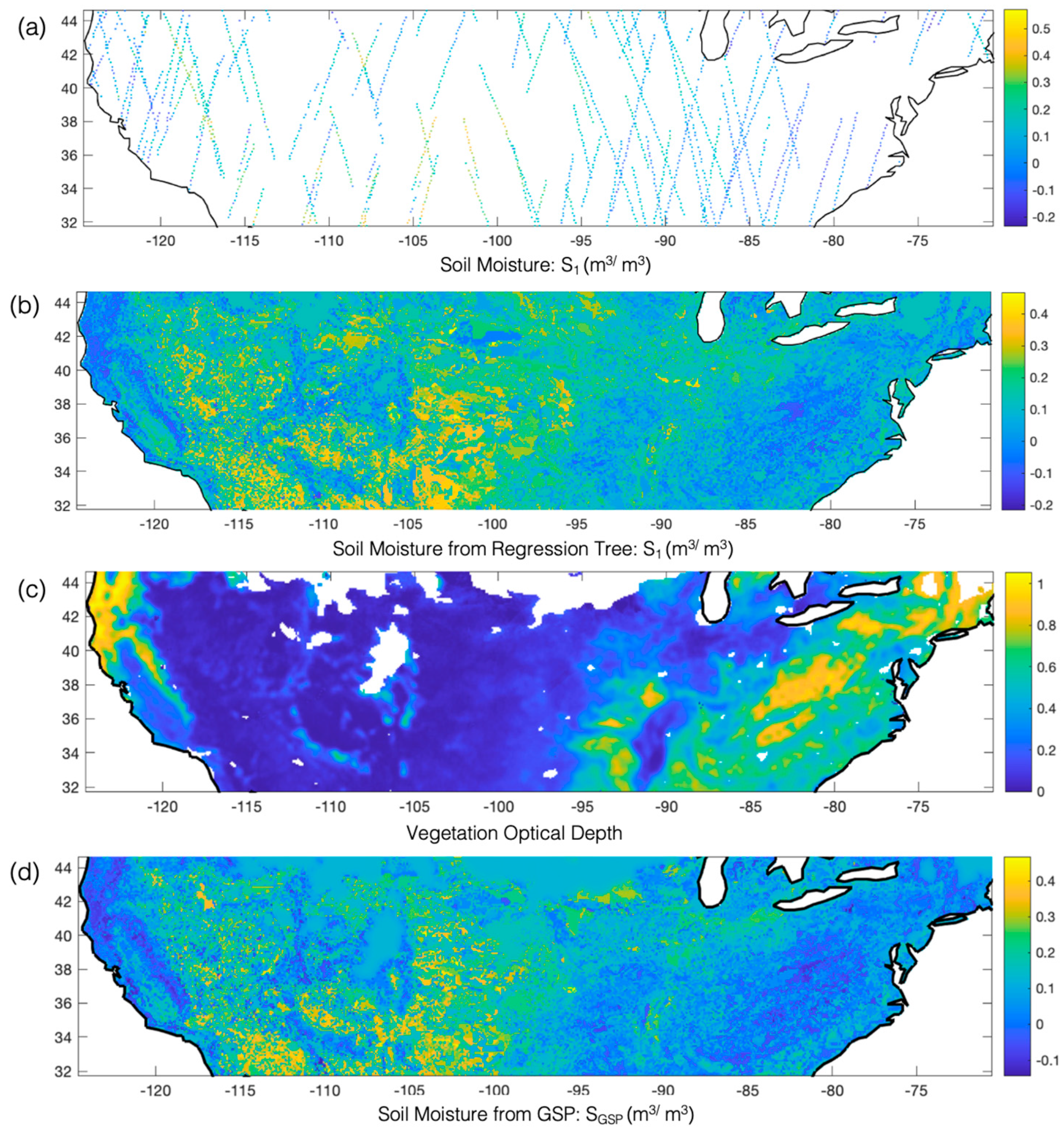
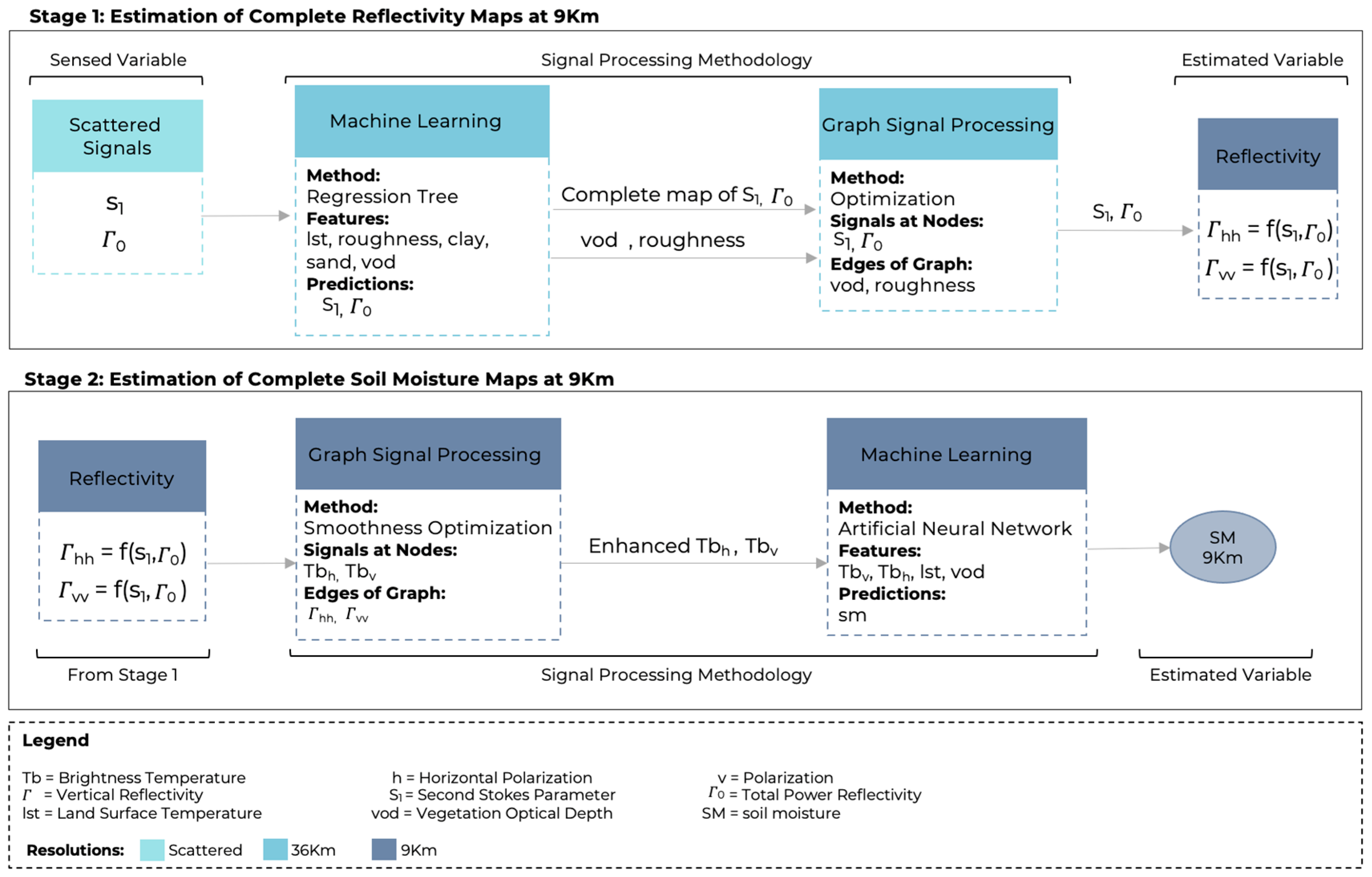
Note that ${\Gamma }_0$ is the calibrated first Stokes parameters following a similar methodology as in the CYGNSS mission, as detailed in [22]. Furthermore, for notation simplicity, we will refer to ${\overline{S}}_1$ here in the document as the normalized second Stokes parameters, $S_1/S_0$. Because ${\overline{S}}_1$ and ${\Gamma }_0$ are sparse, we obtain initial complete maps by implementing a regression tree that takes into consideration vegetation optical depth (VOD) and roughness coefficient information. In the context of this GNSS-R processing using the SMAP radar instrument, the specific characteristics of the instrument minimize the impact of the incidence angle variations on measurements due to its limited range (37.5–42.5°). Consequently, the incidence angle was not included in the machine learning analysis. However, in contrast, for other GNSS-R missions where the incidence angle has a larger variation range, its influence becomes significantly more pronounced, substantially affecting data quality and accuracy. Both ancillary data and validation sources for our algorithms are provided by the SMAP mission. This methodical alignment of both our input and validation datasets is a critical aspect of our study since they belong to the same mission and thus guarantee that the performance metrics we use are not only appropriate but also accurately reflective of the terrain and vegetation characteristics monitored by SMAP. In brief, our method consists of the following steps:

• A machine learning (ML) approach is employed to learn the complex nonlinear relations between geophysical information (e.g., VOD, roughness, LST, and clay and sand composition) with ${\overline{S}}_1$ and ${\Gamma }_0$;
• Complete maps of ${\overline{S}}_1$ and ${\Gamma }_0$ are retrieved from the sparse data using the model learned in step 1;
• Implementing our GSP method, ${\overline{S}}_1$ and ${\Gamma }_0$ maps are improved using VOD and roughness as profiles to determine the graph’s edge weights;
• Reflectivity maps are generated using ${\overline{S}}_1$ and ${\Gamma }_0$ from step 3;
• The calculated reflectivity maps (${\Gamma }_{hh}, { \Gamma }_{vv}$) from step 4 are used as graph profiles to disaggregate $T_b$ at 9 km;
• Brightness temperatures obtained from step 5 are used to estimate SM values that are then validated using CVS measurements.

Figure 2 depicts the strategy highlighted in the previous steps. The methodology to obtain detailed brightness temperature maps vital for soil moisture evaluations will be explained in the subsequent paragraphs.

• Step 1. Developing an ML Model: Sparse Radiometer Signals with Geophysical Data.

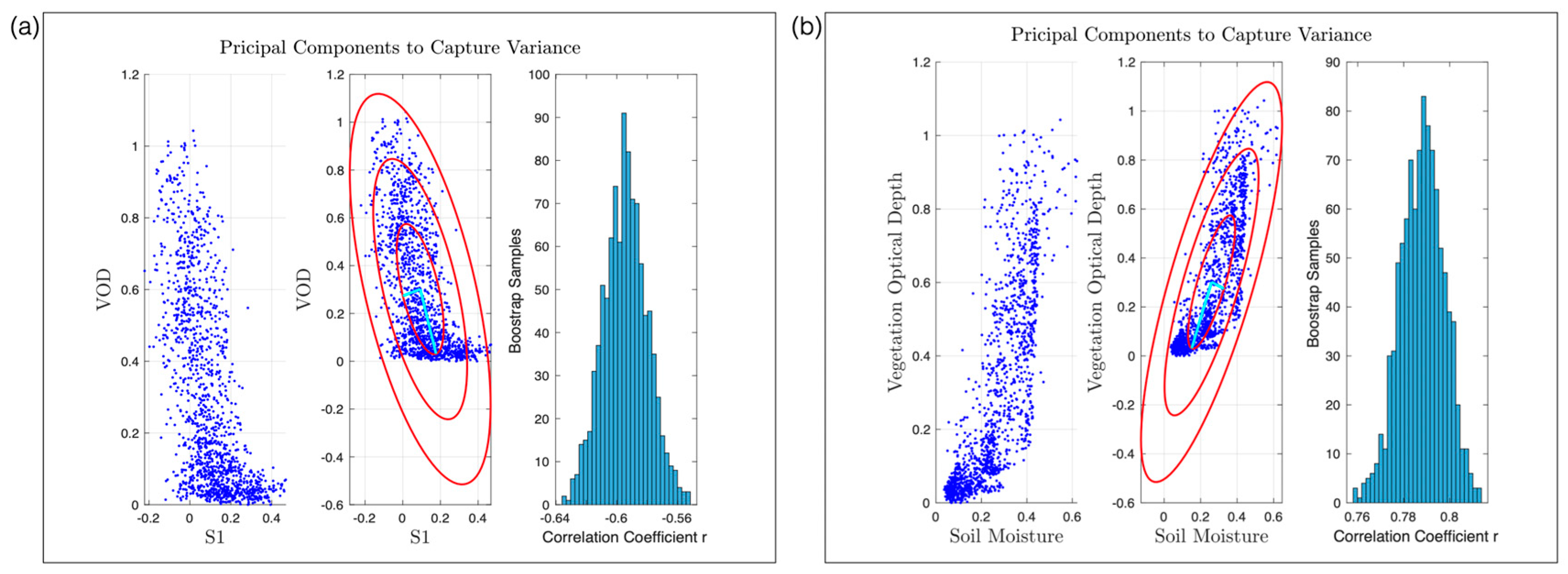
We conducted various correlation analyses and experimented with multiple regression models to select geophysical variables that significantly influence the estimation of ${\overline{S}}_1$ and ${\Gamma }_0$. Remote-sensed metrics, notably LST and VOD, showcased a strong correlation with soil moisture and ${\overline{S}}_1$, as shown in Figure 3. When terrain variables like temperature and vegetation optical depth (VOD) show consistency across adjacent nodes, they form a solid foundation for soil moisture estimation. This reliability stems from the established, statistically significant correlation these variables share with soil moisture levels and the second Stokes parameter. It is noteworthy, however, that this relationship is not strictly linear, indicating a more complex interaction between these terrain variables and SM. Consequently, they became integral to our regression exploration. Recognizing the benefits of regularization and the presence of both linear and nonlinear associations among our variables, we adopted the regression tree ML framework for the estimation of detailed maps of ${\overline{S}}_1$ and ${\Gamma }_0$.

Unlike polynomial regression, regression trees inherently accommodate complex variable interactions through their structure, which can be effectively managed to prevent overfitting via tree pruning and setting depth constraints. These methods, specific to regression trees, offered a significant advantage by allowing the model to be finely tuned to the characteristics of the terrain variables. Within this regression tree (RT) framework, we scrutinized how each variable, both individually and collectively, impacted the accuracy of soil moisture predictions. Variables were primarily selected based on their statistical significance, as evidenced by high correlation values from regression analysis. The final selection of input features in Equation (6), which includes VOD, roughness coefficient, LST, clay, and sand, was grounded both on their performance and their alignment with real-world physical factors.

$$\begin{gathered} S_1=\mathit{RT}\left(\mathit{VOD}, \mathit{roughness}, \mathit{LST}, \mathit{clay},\mathit{sand}\right), \\ {\Gamma }_0=\mathit{RT}(\mathit{VOD}, \mathit{roughness}, \mathit{LST}, \mathit{clay},\mathit{sand}) \end{gathered}$$

(6)

During the training phase, we utilized the known ${\overline{S}}_1$ and ${\Gamma }_0$ data to optimize the RT parameters by reducing the loss function. A significant advantage of our approach is RT’s natural ability to eliminate the need for feature scaling, making data normalization or standardization unnecessary. To implement the RT concept effectively, we utilized established machine learning packages known for their comprehensive features in conducting correlation analyses and optimizing regression trees to enhance the R² performance metric. Moreover, the inherent interpretability of RT models provided a clear insight into decision-making based on feature values. Once the RT parameters were refined, we evaluated their performance in the model’s validation phase using a k-fold validation technique to guarantee a thorough assessment of its efficacy.

• Step 2: Generating complete maps for ${\overline{S}}_1$ and ${\Gamma }_0$ using the model learned from Step 1.

Following the strategy proposed in Figure 2, SMAP-R offers sparse measurements of ${\overline{S}}_1$ and ${\Gamma }_0$, which can be aligned with geophysical variables like VOD, roughness coefficient, LST, clay, and sand. After training the RT, we employed global scale maps of terrain data, VOD, and LST to generate comprehensive maps of ${\overline{S}}_1$ and ${\Gamma }_0$. The non-parametric characteristic of RTs ensures the model’s suitability to project ${\overline{S}}_1$ and σ values, irrespective of the statistical attributes of the terrain variables. Furthermore, the RT method exhibits commendable L2 regularization efficiency, especially with interrelated independent variables, thereby providing a reliable initial estimation of complete ${\overline{S}}_1$ and ${\Gamma }_0$ maps.

• Step 3: Improving ${\overline{S}}_1$ and ${\Gamma }_0$ baseline estimations with GSP methods.

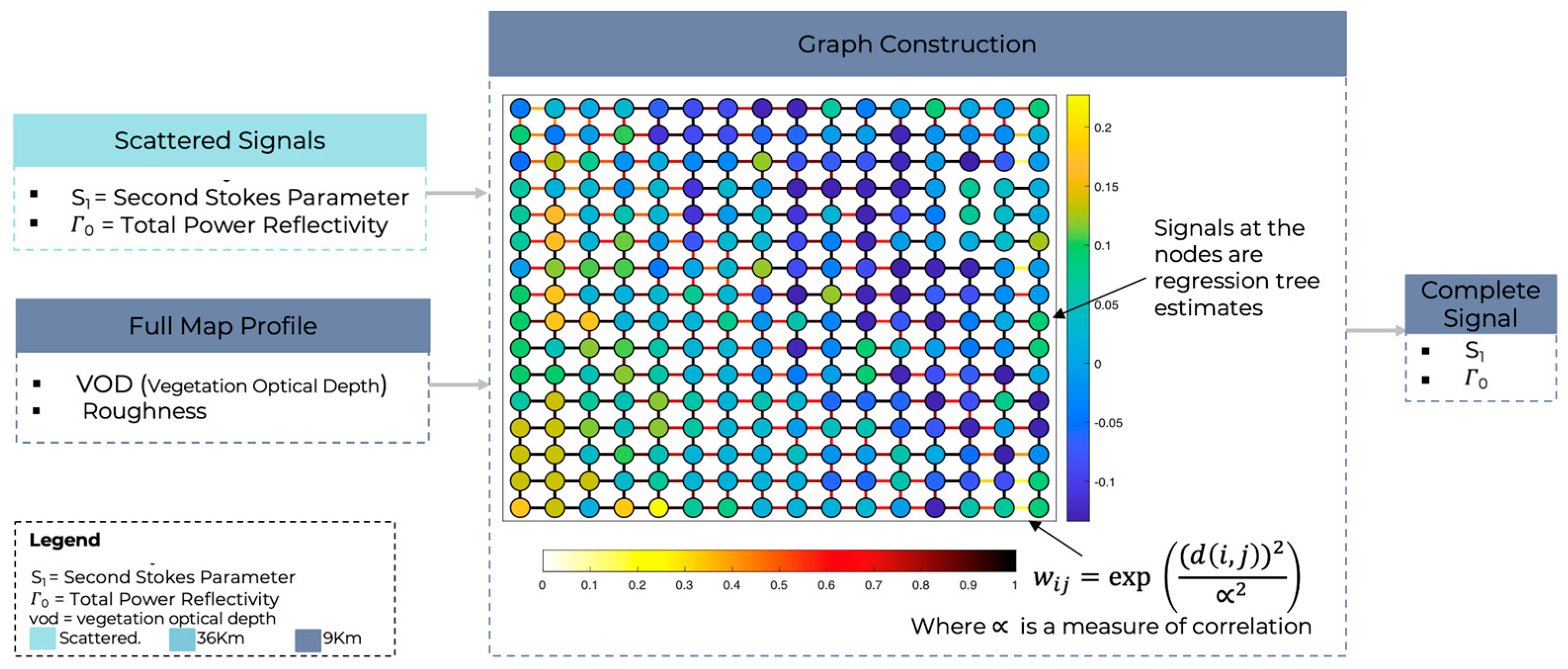
In our experimental setup, the initial graph signals at the nodes represent the interpolated ${\overline{S}}_1$ and ${\Gamma }_0$ derived from step 2, with the edges between the nodes reflecting the terrain attributes. The aim is twofold: firstly, to integrate terrain features with the signals, and secondly, to enhance the estimation of ${\overline{S}}_1$ and ${\Gamma }_0$ by leveraging neighboring nodes with analogous characteristics. This approach also aims to refine and smooth the signal at the nodes, as elaborated below:

(A)

Graph Construction

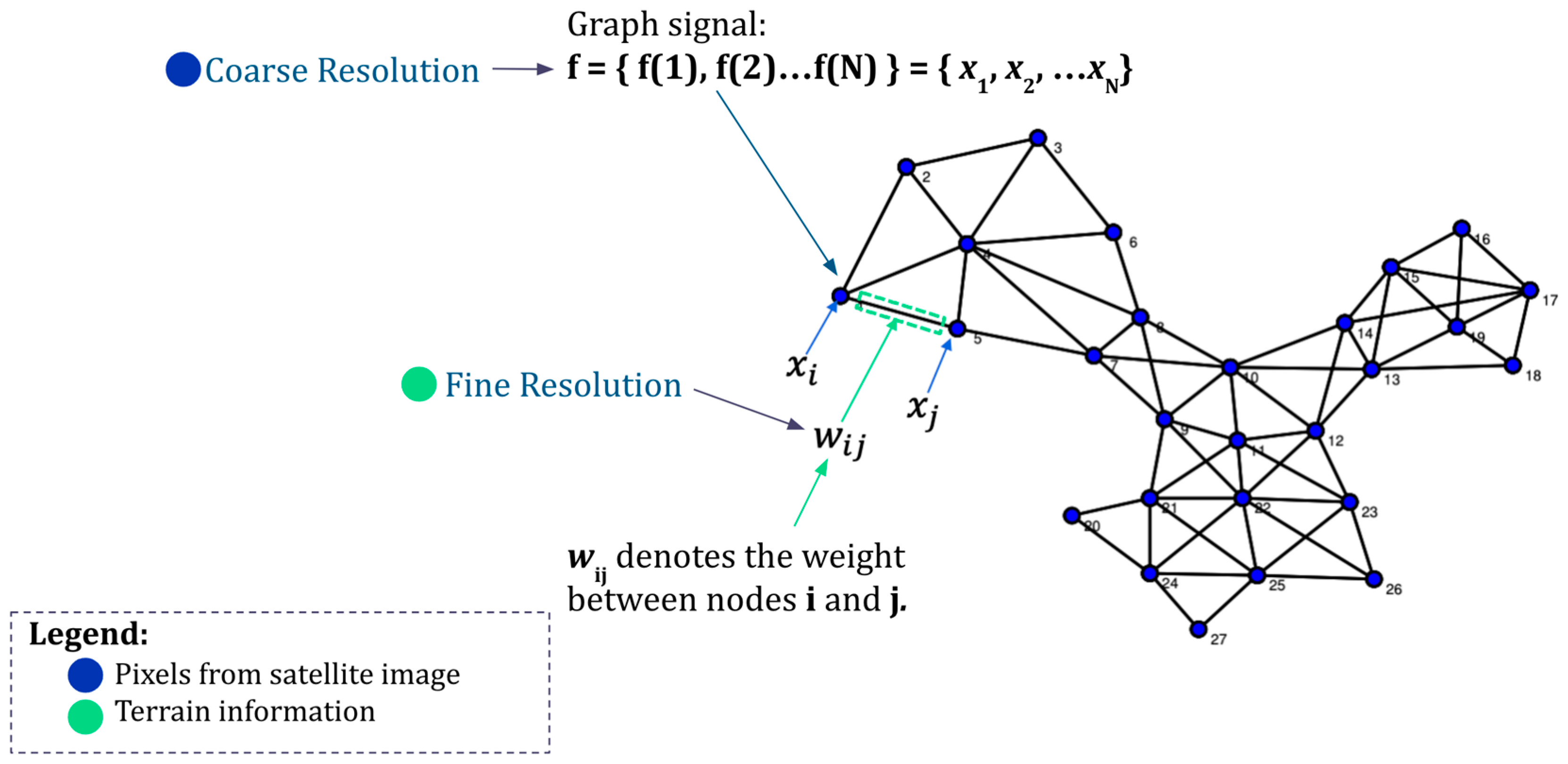
• Graph Signal: Our proposed GSP methodology uses ${\overline{S}}_1$ and ${\Gamma }_0$ from step 2 as the baseline graph signals and terrain data to compute the edges of the graph, as shown in Figure 4. During our analysis, the graph signals are represented by the form $S_1={\left[x_1,x_2, \dots , x_N\right]}^T$ and ${\Gamma }_0={\left[y_1,y_2, \dots , y_N\right]}^T$;
• Edge Weights: Our graph construction method assigns edge weights based on Euclidean distance and statistical correlations among the signal at the nodes and terrain information [23]. From the correlation analysis, the graph construction for ${\overline{S}}_1$ will incorporate edges influenced by VOD, while for ${\Gamma }_0$, the edges will be determined by the roughness coefficient. For $S_1$ graph construction, the edge weights are computed using the Gaussian kernel:

$$w_{i,j}=e^{\left(-\frac{{\left(d_v(i,j)\right)}^2}{{{\alpha }_v}^2}\right)},$$

(7)

where $d_v(i,j)$ represents the difference among VOD values for neighboring nodes $x_{i, }{x}_j$, and ${\alpha }_v$ is a measure of correlation between $S_1$ and VOD. This type of information has the potential to incorporate observed data behavior (correlation) and physical system characteristics (distance).

Analogously, for $\sigma$ graph construction, the graph edges are obtained from

$$w_{i,j}=e^{\left(-\frac{{\left(d_r(i,j)\right)}^2}{{{\alpha }_r}^2}\right)},$$

(8)

In Equation (8), $d_r(i,j)$ represents the difference among roughness coefficient values for neighboring nodes $y_{i, }{y}_j$, and ${\alpha }_r$ is the measure of the correlation between $\sigma$ and roughness values at the node locations.

Note that when the distance $d(i,j)$ becomes much larger than $\alpha$, the corresponding edge weight approaches zero. Therefore, when the terrain information for consecutive nodes is similar, their connection in the graph is strong.

(B)

Graph Optimization

To ensure that our GSP interpolation produces smooth signals on the graph, we follow the optimization problem:

$${\mathit{x}}_{\mathit{opt}}=\underset{\mathit{x}}{\min }{\mathit{x}}^T\mathbf{L}\mathit{x}+\lambda {‖\widehat{\mathit{x}}-\mathit{x}‖}_2^2,$$

(9)

where $\lambda$ serves as the penalty parameter for the baseline interpolated estimation of $\widehat{\mathit{x}}.$ We aim to optimize $\mathit{x}$ such that it remains closely aligned with baseline observations while also ensuring that spatially co-located measurements are like each other, considering terrain characteristics. To enhance the smoothness of the graph, we implemented optimizations on the graph Laplacian $\mathit{L}$ as shown in Equation (9) for both the ${\overline{S}}_1$ and ${\Gamma }_0$ graphs. This optimization approach takes into consideration the local proximity observed in the ${\overline{S}}_1$ and ${\Gamma }_0$ measurements, indicating a likelihood of signal similarity between neighboring observations. By leveraging this similarity, we aim to improve the quality and accuracy of the signal reconstruction process. Ensuring a smoother graph structure, we enable more effective contributions from these signals towards the reconstruction of each other.

Figure 5 illustrates the comprehensive graph signal procedure described to generate ${\overline{S}}_1$ maps leveraging the use of ancillary data. The methodology is articulated based on the steps 1 through 3 outlined previously. Each stage is tailored to streamline the extraction, processing, and eventual rendering of a comprehensive SM map. Figure 5 provides a visual representation of each phase, highlighting the journey from initial regression tree estimates of S1 to the ensuing graph interpolation, which is augmented by VOD. This structured visualization sheds light on the intricate data processing and analytical procedures vital for generating detailed maps from dispersed signals.

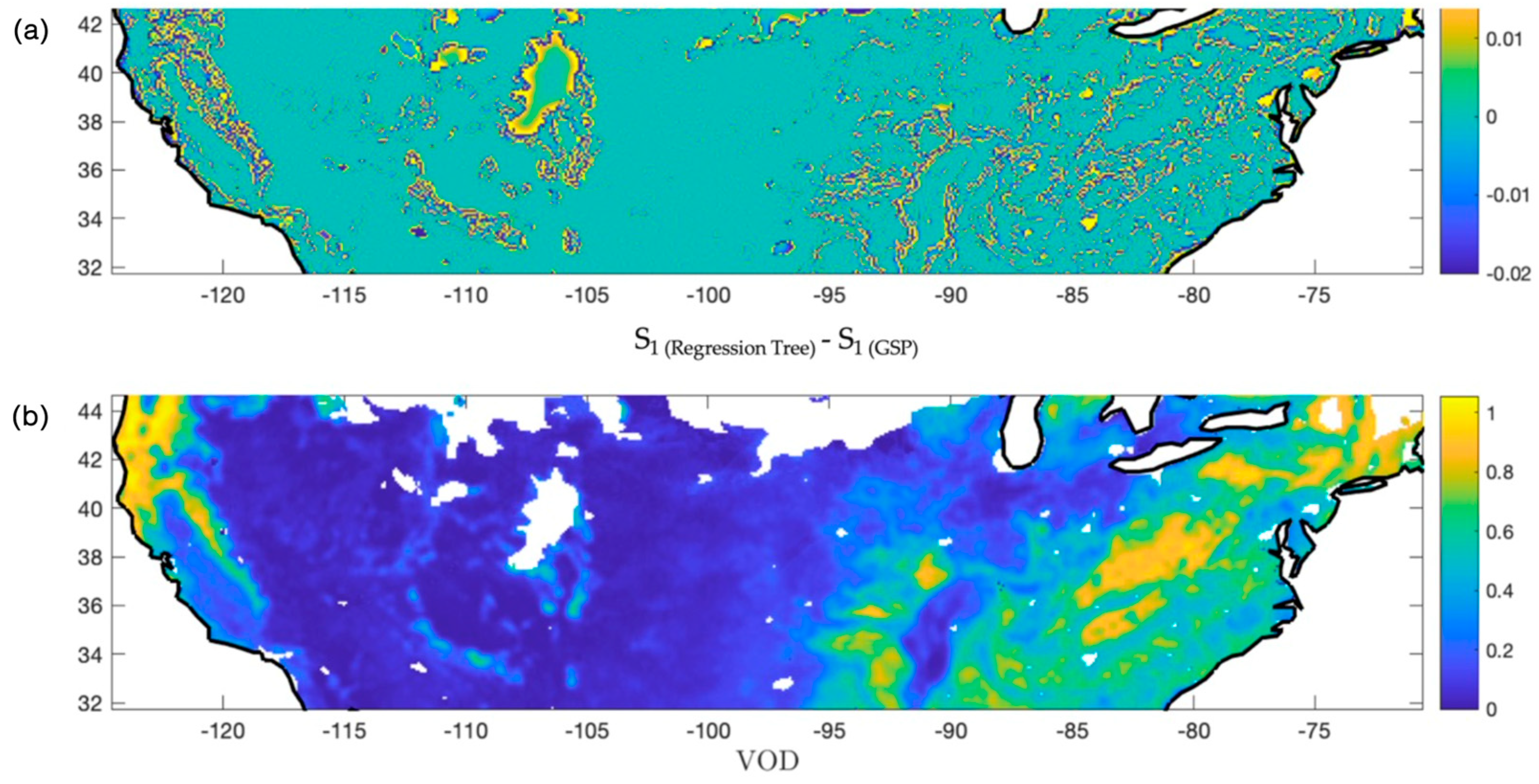
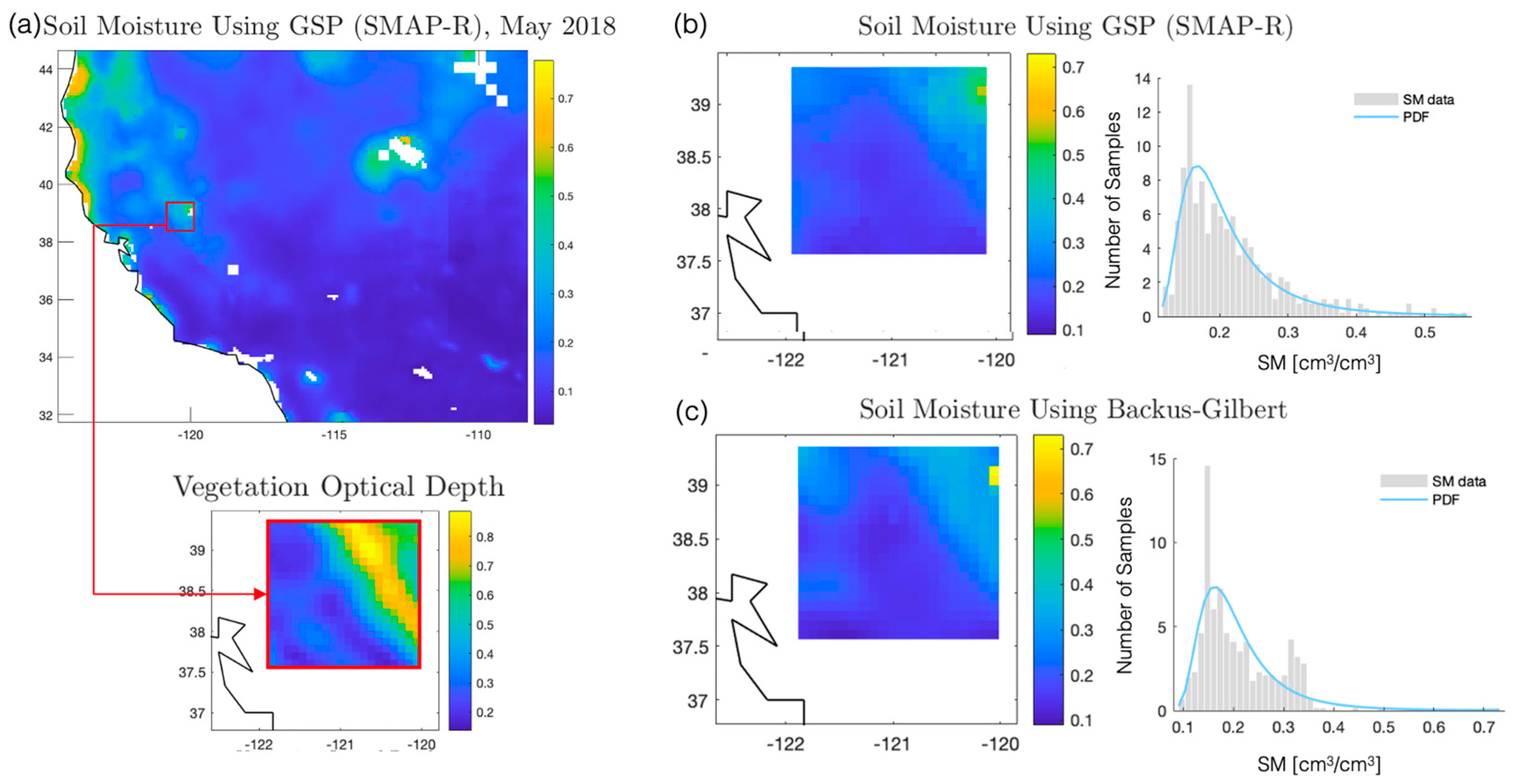
A qualitative validation for the graph signal interpolation using ancillary data is performed by subtracting the final $S_1$ estimates obtained via GSP from those derived from the regression tree methodology (Figure 6). This procedure helps elucidate the regions where VOD information has been utilized to enhance ${\overline{S}}_1$ values. In zones where VOD exhibited uniformity, we denote a smoothing effect on ${\overline{S}}_1$ values. This smoothing is an outcome of the GSP algorithm, which uses the similarity in vegetation optical depth between neighboring areas to enhance the spatial continuity of the ${\overline{S}}_1$ estimates. In contrast, over regions presenting diverse vegetation values, the graph becomes disconnected, leading to an absence of spatial smoothing in ${\overline{S}}_1$ values. This occurs because the GSP algorithm identifies these diverse vegetation characteristics as boundaries and thus does not propagate information across these boundaries. This analysis provides an illustrative and quantifiable demonstration of the efficacy of integrating ancillary information, like VOD, into our GSP methodology. The ability to enhance or moderate the smoothing of ${\overline{S}}_1$ values based on terrain characteristics affirms the strength of the GSP approach. The initial interpolation from the regression tree is key in the described methodology, as it forms the baseline graph signal. The subsequent application of GSP significantly enhances soil moisture estimation accuracy since SM estimates derived from GSP methods surpass those from ML approaches. This is due to the fact that GSP allows for effective regularization by considering observations with similar characteristics. Furthermore, our approach incorporates a multimodal analysis, where multiple physical variables influence or help estimate a measurement. A distinct advantage of using GSP over ML models is that it does not rely heavily on extensive training and validation data. This is particularly beneficial for estimating models of interconnected variables where data availability might be limited.

• Step 4: Estimating reflectivity maps (${\Gamma }_{hh}, { \Gamma }_{vv}$) as functions of ${\overline{S}}_1$ and ${\Gamma }_0$.

The Stokes parameters can be translated into reflectivity measurement using Equation (4). This translation of the first Stokes parameters into reflectivity provides a significant advantage, as it contains crucial information about seasonal variations.

• Step 5: Disaggregating brightness temperature ($T_b$s) using (${\Gamma }_{hh}, { \Gamma }_{vv}$).

To achieve an accurate downscaling of SM to a 9 km resolution, we first augment the spatial resolution of the $T_b$ from 36 km to 9 km, capitalizing on our derived reflectivity signals at the 9 km scale. To facilitate this enhancement, we adopt the signal processing methodology delineated earlier. The GSP method utilizes precomputed reflectivity maps to heighten the resolution of brightness temperatures. Central to this approach is the premise of using reflectivity maps as auxiliary datasets to infer brightness temperatures across distinct spatial coordinates. Within this framework, the signal at each node represents brightness temperatures, and the edge weights interlinking these nodes are modulated by the amplitude of reflectivity. Consequently, the resolution refinement of $T_b$ is significantly augmented with the inclusion of reflectivity maps, representing a distinct advancement over traditional re-gridding techniques or geospatial procedures such as kriging.

5. Soil Moisture Retrieval Results

To derive our SM estimates, our primary aim was to construct the most reliable reflectivity maps, which, when combined with terrain information, would refine the predictions of $T_b$. Leveraging the graph-based methodology, we were able to interpolate reflectivities, effectively accounting for both the similarities in terrain and the unique attributes of vegetation. This precise interpolation of reflectivities allowed the enhancement of Tb resolution, laying a robust groundwork for our subsequent machine learning endeavors in SM estimation. Our choice of the Neural Network (NN) model was deliberate and strategic. This model is calibrated to deduce SM levels, drawing from a combination of $T_b$s, land surface temperatures, and VOD representation vectors—essential elements in our estimation process. The NN model deciphers the inherent patterns within these vectors, promising precise SM-level predictions. Since the estimated $T_b$ obtained from GSP is the input to the NN for the SM estimation, the ML model is not just reliant on $T_b$ but also assimilates the intricate dynamics of terrain and other environmental influencers, reinforcing a comprehensive approach to our SM estimations.

5.1. Soil Moisture from Artificial Neural Network

Our methodology for SM estimation incorporates an NN approach, with the selected input parameters comprising brightness temperatures derived from SMAP observations for both V and H polarizations. Additionally, ancillary data, including land surface temperature and VOD, are incorporated. Our NN model shares operational similarities with the dual-channel algorithm (DCA) described in [28]. By paralleling this methodology, our model leverages the strengths of DCA while providing the additional benefits offered by an NN approach, effectively accounting for multiple environmental variables and increasing the accuracy of the derived SM estimates. In terms of validating our NN-based estimates, they are contrasted against measurements taken from calibration and validation sites (CVS). These sites offer an empirical benchmark to assess the accuracy of our SM estimates and to refine the model as necessary. The subsequent section will provide a detailed analysis of these findings, elucidating the performance of our model and outlining potential avenues for future improvement.

5.2. Results

To evaluate the efficacy of our graph interpolation algorithms and to explore the potential of using them for combining SMAP radiometer and SMAP-R measurements to obtain SM estimates, we conducted a study over the course of 2018. The objective of this study was to compare the SM predictions derived from our methodology against in situ measurements taken from 50 calibration sites used during the SMAP mission (SMAP CalVal) throughout the year (Figure 7). The continuous blue and purple lines, while close, do not match perfectly, indicating a subtle difference in trends. This distinction becomes clearer through the individual data points (represented by crosses), with the blue crosses (SMAP-R) aligning more consistently with calibration/validation (Cal/Val) values. Figure 7 aims to demonstrate the effectiveness of our interpolated estimates, which are not only closer to Cal/Val values but also show a maintained correlation with in situ data, even after the images have been processed for higher resolution. This point is essential, underscoring that our interpolation methods do more than just improve the imagery’s spatial resolution; they also safeguard the data’s accuracy and dependability regarding soil moisture.

Figure 7a presents the outcome of this comparison, juxtaposing the radiometer SM estimates obtained at a resolution of 36 km with the SM estimates derived from the SMAP-R methodology. It is noteworthy that when these estimates are set against the corresponding in situ measurements, the mean values predicted by the SMAP-R approach demonstrate a closer alignment with the validation values. Further, to provide a clear illustration, we selected a validation site to contrast the average soil moisture values derived from in situ measurements with those from SMAP at 9 km resolution, using both the Backus–Gilbert method and our SMAP-R data. Figure 7b highlights that the SMAP-R estimates, generated via the GSP method, align more closely with a specific Tonzi Ranch validation site’s value. This is evident as they approach the 5% confidence interval, depicted by the shaded grey region.

Incorporating VOD in the graph construction process for SM estimation offers multiple enhancements to the quality of the estimates. VOD is a crucial factor in accounting for the effects of vegetation on microwave signals, such as those measured by the SMAP radiometer. Vegetation interacts with microwave radiation through absorption and scattering mechanisms, altering the received signal’s characteristics. Thus, by considering VOD during graph construction, these vegetation-induced effects can be better accounted for, leading to more precise SM estimates, Figure 8. As observed in Figure 8a,b, a greater distinction in VOD values corresponds to enhanced performance of SMAP-R when compared with SMAP36. This underscores the significance of the graph method, which facilitates the interpolation of values, incorporating terrain information inherent to the signal characteristics.

It becomes evident that there exists a discernible contrast in absolute error when contrasting SMAP-R estimations against SMAP36 used as ground truth, as shown in Figure 8. Notably, the performance demonstrates improvement when the average vegetation optical depth (VOD) of the observations is higher. This trend strongly suggests that the inclusion of VOD information contributes significantly to enhancing the accuracy of soil moisture (SM) value estimations. VOD serves as a proxy for vegetation water content, offering indirect insights into the vegetation layer’s influence on soil moisture dynamics. This includes how vegetation can retain moisture and affect the local microclimate, thereby influencing soil moisture levels. In Figure 9, a comprehensive soil moisture measurement map for May 2018 is shown (Figure 9a). Within a selected region showcasing variable VOD (Figure 9a), differences are evident in interpolation estimates between SMAP-R (9b) and SMAP derived from the Backus–Gilbert (SM_BG) interpolation technique (9c). While there are similarities, it is evident that the value distribution in SM_BG exhibits a tendency for over-smoothing. Conversely, SMAP-R presents a broader spectrum of values, which are more congruent with the characteristics of the VOD.

From the highlighted region in Figure 9, an in situ sensor at the core validation site was selected to compare the fidelity of our SMAP-R estimates with that of SM_BG. The correlation coefficient, as depicted in Figure 10, served as a pertinent metric to substantiate that, over the course of 2018, SMAP-R estimates exhibited closer alignment with the readings from the validation site. The choice of correlation as a metric is justified by its ability to quantify linear relationships, ensuring that both the magnitude and directionality of deviations across measurements are considered. The decision to focus on vegetation stems from the understanding that variations in vegetation optical depth (VOD) reveal environmental dynamics, which are key to achieving precise soil moisture estimations. It is important to highlight that SMAP-R measurements shed light on the conditions of the underlying soil, as the bistatic radar measurements, or reflectometry, predominantly capture a strong single bounce signal originating from the soil’s surface. By incorporating VOD information into our graph model, we are leveraging the natural physical characteristics of the terrain. This approach enables the isolation of the soil’s single bounce signal, which is influenced by its roughness and soil moisture (SM), from the volumetric scattering effects of vegetation. This synthesis of data not only enhances the richness of our dataset but also ensures that our interpolation efforts are deeply rooted in the physical reality of the targeted area, providing a more accurate representation of soil moisture levels.

Figure 11 presents a compelling comparison of error performance between two methodologies for SM estimation—the traditional SMAP at a resolution of 36 km and the novel SMAP-R. This comparison is achieved by directly contrasting the SM estimates from these methodologies against the same set of in situ measurements. A noteworthy observation from this comparison is that the SMAP-R methodology provides superior estimates, as evidenced by its lower error rates. The improved performance of SMAP-R can be attributed to its innovative approach that leverages SMAP GNSS-R data for disaggregating brightness temperature and GSP, a technique that introduces a novel dimension to SM estimation by integrating terrain information into the interpolation and signal processing tasks. In terms of error calculations, we observed an 11.8% reduction in the Root Mean Square Error (RMSE) compared to the SMAP36 data. Additionally, there was a significant 14.7% reduction in uncentered RMSE (uRMSE) across the entire year of 2018, covering all 50 SMAP validation sites.

In Figure 12, we present a comparative analysis of RMSE errors between SM36 and SMAPR across the CalVal sites throughout the year 2018, alongside the corresponding VOD standard deviation. Notably, the plot reveals a compelling relationship: when the VOD standard deviation is elevated, signifying greater variation in vegetation, the performance of SMAPR notably improves. This improvement can be attributed to the graph-based method’s ability to effectively consider and accommodate temporal variations in terrain characteristics during signal interpolation.

These results emphasize the effectiveness of our approach in enhancing the accuracy of geophysical parameter estimation, especially in highly vegetated areas. The use of terrain information in GSP enables the model to consider spatial continuity and context, which can significantly enhance the accuracy of SM estimates. This innovative combination of disaggregating brightness temperature using GNSS-R data and the application of GSP proves to be a powerful tool for refining SM estimations. Moving away from conventional approaches, our GSP-based method enables more effective integration and interpolation of ancillary data across different spatio-temporal scales, representing a major step forward in remote sensing applications. In our research using SMAP-R data, we have discovered new strategies for addressing the challenges presented by datasets characterized by significant gaps in both time and space, leveraging terrain features as effective proxies for interpolation.

6. Conclusions

GSP emerges as an innovative approach for the integration of multi-resolution data within the field of remote sensing applications. This methodology leverages ancillary data to perform efficient interpolation of observations from coarser resolutions and sparse signals. Furthermore, GSP presents a viable alternative for simultaneous analysis of data originating from diverse spatio-temporal resolutions, thus offering a novel approach to signal estimation on graphs.

The work undertaken using the SMAP-R data has offered the opportunity to delve into the utilization of the GSP approach on an intricately challenging dataset, which is characterized by significant temporal and spatial sparsity. Through this endeavor, we have successfully demonstrated the incremental value offered by the incorporation of multi-instrument data for improved estimation of geophysical parameters. This is substantiated by our findings that enhancing SMAP radiometer data with SMAP-R data results in superior SM estimations, particularly over vegetated areas characterized by elevated VOD.

Our results emphasize the potential advantages of the SMAP-R methodology in the context of Soil Moisture (SM) estimation, with notable reductions in the Root Mean Square Error (RMSE) of 11.8% and unbiased RMSE (uRMSE) of 14.7% compared to traditional radiometer estimates. The improved precision of SMAP-R estimates, compared to traditional radiometer estimates, opens up new opportunities for ongoing research and potential advancements in SM measurement methodologies. Continual comparative analyses with in situ measurements play a crucial role, serving as essential benchmarks for refining these methodologies and algorithms further. As a result, we achieve more accurate and reliable SM estimations, which have the potential to significantly enhance various domains, including environmental science, agriculture, and climate studies.

References

1. The Global Climate Observing System (GCOS) What are Essential Climate Variables? Available online: https://gcos.wmo.int/en/essential-climate-variables/about (accessed on 26 September 2023).
2. Eroglu, O.; Kurum, M.; Boyd, D.; Gurbuz, A.C. High spatio-temporal resolution cygnss soil moisture estimates using artificial neural networks. Remote Sens. 2019, 11, 2272. [Google Scholar] [CrossRef]
3. Dobriyal, P.; Qureshi, A.; Badola, R.; Hussain, S.A. A review of the methods available for estimating soil moisture and its implications for water resource management. J. Hydrol. 2012, 458–459, 110–117. [Google Scholar] [CrossRef]
4. Kerr, Y.H.; Waldteufel, P.; Richaume, P.; Wigneron, J.P.; Ferrazzoli, P.; Mahmoodi, A.; al Bitar, A.; Cabot, F.; Gruhier, C.; Juglea, S.E.; et al. The SMOS Soil Moisture Retrieval Algorithm. IEEE Trans. Geosci. Remote Sens. 2012, 50, 1384–1403. [Google Scholar] [CrossRef]
5. Entekhabi, D.; Njoku, E.G.; O’Neill, P.E.; Kellogg, K.H.; Crow, W.T.; Edelstein, W.N.; Entin, J.K.; Goodman, S.D.; Jackson, T.J.; Johnson, J.; et al. The Soil Moisture Active Passive (SMAP) Mission. Proc. IEEE 2010, 98, 704–716. [Google Scholar] [CrossRef]
6. Narasimhan, B.; Srinivasan, R. Development and evaluation of Soil Moisture Deficit Index (SMDI) and Evapotranspiration Deficit Index (ETDI) for agricultural drought monitoring. Agric. For. Meteorol. 2005, 133, 69–88. [Google Scholar] [CrossRef]
7. Entekhabi, D.; Yueh, S.H.; O’neill, P.E.; Kellogg, K.H.; Allen, A.M.; Bindlish, R.; Brown, M.E.; Chan, S.T.K.; Colliander, A.; Crow, W.T.; et al. SMAP Handbook–Soil Moisture Active Passive: Mapping Soil Moisture and Freeze/Thaw from Space. 2014. Available online: https://www.semanticscholar.org/paper/SMAP-Handbook%E2%80%93Soil-Moisture-Active-Passive%3A-Mapping-Entekhabi-Yueh/8ba9c2e6277b1960c36192f68dd50e0041054fe8 (accessed on 14 February 2024).
8. Ramsey, S. NASA Soil Moisture Radar Ends Operations, Mission Science Continues. Available online: http://www.nasa.gov/press-release/nasa-soil-moisture-radar-ends-operations-mission-science-continues (accessed on 14 February 2024).
9. Munoz-Martin, J.F.; Rodriguez-Alvarez, N.; Bosch-Lluis, X.; Oudrhiri, K. Analysis of polarimetric GNSS-R Stokes parameters of the Earth’s land surface. Remote Sens. Environ. 2023, 287, 113491. [Google Scholar] [CrossRef]
10. Raney, R.K. Polarimetric Portraits. Earth Space Sci. 2021, 8, e2021EA001768. [Google Scholar] [CrossRef]
11. Rodriguez-Alvarez, N.; Misra, S.; Morris, M. The Polarimetric Sensitivity of SMAP-Reflectometry Signals to Crop Growth in the U.S. Corn Belt. Remote Sens. 2020, 12, 1007. [Google Scholar] [CrossRef]
12. Munoz-Martin, J.F.; Rodriguez-Alvarez, N.; Bosch-Lluis, X.; Oudrhiri, K. Stokes Parameters Retrieval and Calibration of Hybrid Compact Polarimetric GNSS-R Signals. IEEE Trans. Geosci. Remote Sens. 2022, 60, 1–11. [Google Scholar] [CrossRef]
13. Munoz-Martin, J.F.; Bosch-Lluis, X.; Rodriguez-Alvarez, N.; Oudrhiri, K. Calibration Strategy for Compact Polarimetric GNSS-R Instruments. IEEE Trans. Geosci. Remote Sens. 2023, 61. [Google Scholar] [CrossRef]
14. Rodriguez-Alvarez, N.; Munoz-Martin, J.F.; Bosch-Lluis, X.; Oudrhiri, K.; Entekhabi, D.; Colliander, A. The first polarimetric GNSS-Reflectometer instrument in space improves the SMAP mission’s sensitivity over densely vegetated areas. Sci. Rep. 2023, 13, 1–12. [Google Scholar]
15. Clarizia, M.P.; Pierdicca, N.; Costantini, F.; Floury, N. Analysis of CYGNSS Data for Soil Moisture Retrieval. IEEE J. Sel. Top. Appl. Earth Obs. Remote Sens. 2019, 12, 2227–2235. [Google Scholar] [CrossRef]
16. Chew, C.C.; Small, E.E. Soil Moisture Sensing Using Spaceborne GNSS Reflections: Comparison of CYGNSS Reflectivity to SMAP Soil Moisture. Geophys. Res. Lett. 2018, 45, 4049–4057. [Google Scholar] [CrossRef]
17. Al-Khaldi, M.M.; Johnson, J.T.; O’Brien, A.J.; Balenzano, A.; Mattia, F. Time-Series Retrieval of Soil Moisture Using CYGNSS. IEEE Trans. Geosci. Remote Sens. 2019, 57, 4322–4331. [Google Scholar] [CrossRef]
18. Sanfeliu, A.; Alquézar, R.; Andrade, J.; Climent, J.; Serratosa, F.; Vergés, J. Graph-based representations and techniques for image processing and image analysis. Pattern Recognit. 2002, 35, 639–650. [Google Scholar] [CrossRef]
19. Jimenez-Sierra, D.A.; Benítez-Restrepo, H.D.; Vargas-Cardona, H.D.; Chanussot, J. Graph-Based Data Fusion Applied to: Change Detection and Biomass Estimation in Rice Crops. Remote Sens. 2020, 12, 2683. [Google Scholar] [CrossRef]
20. Sun, Y.; Lei, L.; Li, X.; Tan, X.; Kuang, G. Structure Consistency-Based Graph for Unsupervised Change Detection With Homogeneous and Heterogeneous Remote Sensing Images. IEEE Trans. Geosci. Remote Sens. 2022, 60, 1–21. [Google Scholar] [CrossRef]
21. Sun, Y.; Lei, L.; Guan, D.; Li, M.; Kuang, G. Sparse-Constrained Adaptive Structure Consistency-Based Unsupervised Image Regression for Heterogeneous Remote-Sensing Change Detection. IEEE Trans. Geosci. Remote Sens. 2022, 60, 1–14. [Google Scholar] [CrossRef]
22. Sun, Y.; Lei, L.; Guan, D.; Kuang, G.; Member, S.; Liu, L. Graph Signal Processing for Heterogeneous Change Detection-Part I: Vertex Domain Filtering. arXiv 2022, arXiv:2208.01881. [Google Scholar]
23. Cardona, J.G.; Ortega, A.; Rodriguez-Alvarez, N. Graph-Based Interpolation for Remote Sensing Data. In Proceedings of the 2022 30th European Signal Processing Conference (EUSIPCO), Belgrade, Serbia, 29 August–2 September 2022; pp. 1791–1795. [Google Scholar]
24. Ortega, A. Introduction to Graph Signal Processing, 1st ed.; Cambridge University Press: Cambridge, UK, 2021. [Google Scholar]
25. Garcia-Cardona, J.; Ortega, A.; Rodriguez-Alvarez, N. Downscaling SMAP Soil Moisture with Ecostress Products using a Graph-Based Interpolation Method. In International Geoscience and Remote Sensing Symposium (IGARSS); Institute of Electrical and Electronics Engineers Inc.: New York, NY, USA, 2022; Volume 2022, pp. 6169–6172. [Google Scholar]
26. Stankovic, L.; Mandic, D.P.; Dakovic, M.; Kisil, I.; Sejdic, E.; Constantinides, A.G. Understanding the Basis of Graph Signal Processing via an Intuitive Example-Driven Approach [Lecture Notes]. IEEE Signal Process Mag. 2019, 36, 133–145. [Google Scholar] [CrossRef]
27. Rodriguez-Alvarez, N.; Misra, S.; Podest, E.; Morris, M.; Bosch-Lluis, X. The Use of SMAP-Reflectometry in Science Applications: Calibration and Capabilities. Remote Sens. 2019, 11, 2442. [Google Scholar] [CrossRef]
28. Colliander, A.; Reichle, R.H.; Crow, W.T.; Cosh, M.H.; Chen, F.; Chan, S.; Das, N.N.; Bindlish, R.; Chaubell, J.; Kim, S.; et al. Validation of Soil Moisture Data Products From the NASA SMAP Mission. IEEE J. Sel. Top. Appl. Earth Obs. Remote Sens. 2022, 15, 364–392. [Google Scholar] [CrossRef]
Figure 1. Illustrating the utility of graphs for data integration: nodes represent coarse-resolution dataset elements, edges incorporate additional correlated information, and enhanced resolution can be achieved through high-resolution edge definitions. Adopting this method allows us to interpret a satellite image as a grid graph. In this framework, f = {xi, xj …. xN} represents the coarsely sensed variable and graph signal, while the connections (edges = Wi,j) between the nodes (pixels: xi, xj) reflect similarities in the terrain, such as altitude variations.
Remotesensing 16 01397 g001
Figure 2. Graph construction and optimization strategy for 9 km resolution soil moisture estimation, where S ¯ 1 is the normalized second Stokes parameter.
Remotesensing 16 01397 g002
Figure 3. Quantitative evaluation of soil moisture and S ¯ 1 correlations with additional variables: (a) Analysis of the relationship between S ¯ 1 and vegetation optical depth (VOD). (b) Analysis of the relationship between soil moisture and VOD.
Remotesensing 16 01397 g003
Figure 4. Graph construction for the Stokes parameters ( S ¯ 1 ) and the total power reflectivity ( Γ 0 ) with the inclusion of terrain data for defining edges. The weight matrix gauges the degree of association between adjacent signal observations of ( S ¯ 1 ) and Γ 0 .
Remotesensing 16 01397 g004
Figure 5. Progression of scatter signal processing and mapping using GSP: (a) Scatter signal retrieval, focusing on the second Stokes parameter S ¯ 1 during the first quarter of 2018. (b) Initial estimation of complete map, using a regression tree method that incorporates ancillary data—roughness coefficient, sand, and clay. (c) Vegetation optical depth map employed for defining graph edges. (d) Final graph representation, where the linkages between neighboring nodes with assigned S1 values are enriched by the incorporation of vegetation optical depth data. This sequential methodology helps towards a comprehensive and accurate mapping of the scattered signals.
Remotesensing 16 01397 g005
Figure 6. (a) Comparison of final S ¯ 1 estimates derived from GSP and the RT methodology. In regions exhibiting diverse vegetation values, the graph representation becomes disconnected, leading to a noticeable absence of spatial smoothing in S ¯ 1 values. Thus, the difference between estimates from GSP and RT becomes more noticeable. (b) VOD map influencing the graph interpolation.
Remotesensing 16 01397 g006
Figure 7. (a) A comparative analysis of soil moisture estimates derived from SMAP at a resolution of 36 km and SMAP-R, set against in situ data collected over the course of 2018. The blue line, representing SMAP-R, has a slope closer to one, indicating a better alignment with the validation results compared to the purple line, which represents SMAP36. (b) Soil moisture (m3/m3) comparison at a validation site: in situ measurements versus SMAP at 9 km, including Backus–Gilbert and our SMAP-R estimates. The plots provide a visual representation of the performance of these two methodologies in relation to actual on-ground measurements.
Remotesensing 16 01397 g007
Figure 8. (a) Comparative SMAP-R performance with variations on VOD. (b) Comprehensive error analysis for SM estimates across 50 distinct locations over a year, highlighting the improvements in accuracy when VOD is intensively incorporated into the interpolation process.
Remotesensing 16 01397 g008
Figure 9. (a) Comprehensive soil moisture map for May 2018. Within a highlighted region with variable VOD. (b) Statistical distribution of interpolation estimates for SMAP-R. (c) Statistical distribution for SMAP using the Backus–Gilbert technique. A discernible spatial smoothing is evident in (c), while (b) showcases values that align more closely with VOD characteristics.
Remotesensing 16 01397 g009
Figure 10. Scatter plot comparing in situ CalVal soil moisture readings with estimates from SMAP-R, SMAP, and SM_BG. The x-axis displays soil moisture estimates obtained through interpolation, while the y-axis shows corresponding CalVal readings. Linear regression lines for each method illustrate the degree of correlation, with correlation coefficients (R) indicating the strongest correlation for SMAP-R (R = 0.71), followed by SM_BG (R = 0.63) and SMAP (R = 0.57).
Remotesensing 16 01397 g010
Figure 11. A direct comparison of soil moisture estimates against CalVal values for selected sites. (a) Illustrates the difference of soil moisture estimates derived from SMAP at a resolution of 36 km compared to CalVal values. (b) Contrasts the accuracy of soil moisture estimates from the innovative SMAP-R methodology against the same CalVal measurements. (c) Vegetation optical depth for selected sites.
Remotesensing 16 01397 g011
Figure 12. RMSE comparison between SM 36 and validation data. (b) SMAPR vs. validation data. (c) VOD standard deviation for 2018 CalVal Sites.
Remotesensing 16 01397 g012
Disclaimer/Publisher’s Note: The statements, opinions and data contained in all publications are solely those of the individual author(s) and contributor(s) and not of MDPI and/or the editor(s). MDPI and/or the editor(s) disclaim responsibility for any injury to people or property resulting from any ideas, methods, instructions or products referred to in the content.