Coseismic and Early Postseismic Deformation Mechanism Following the 2021 Mw 7.4 Maduo Earthquake: Insights from Satellite Radar Interferometry and GPS

 ,
,  ,
,  , and
, and
Abstract
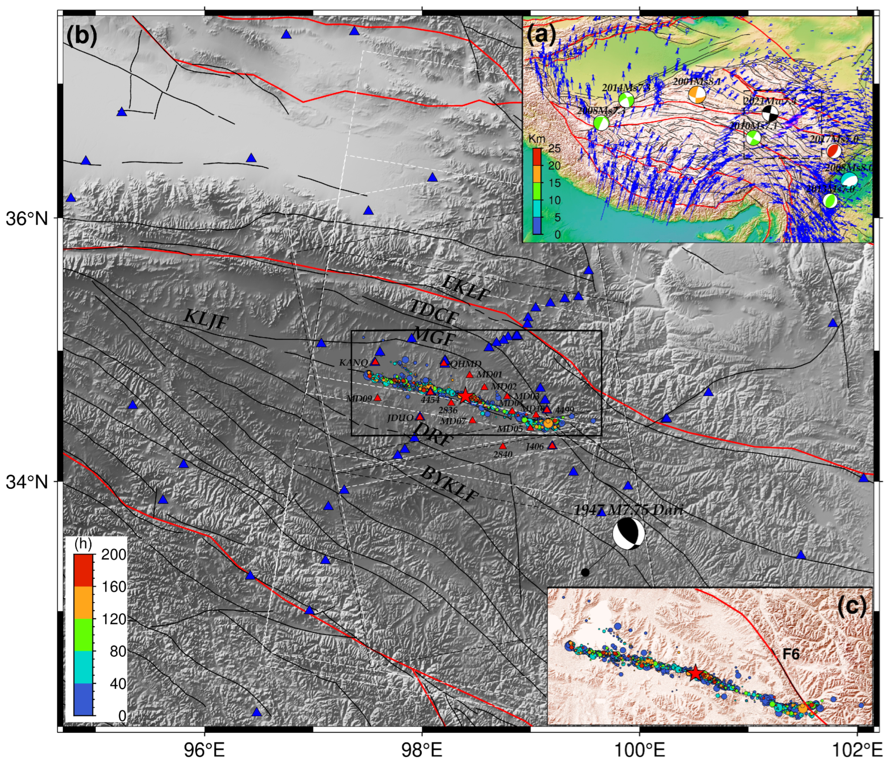
:1. Introduction

2. Methodology and Data Preprocessing
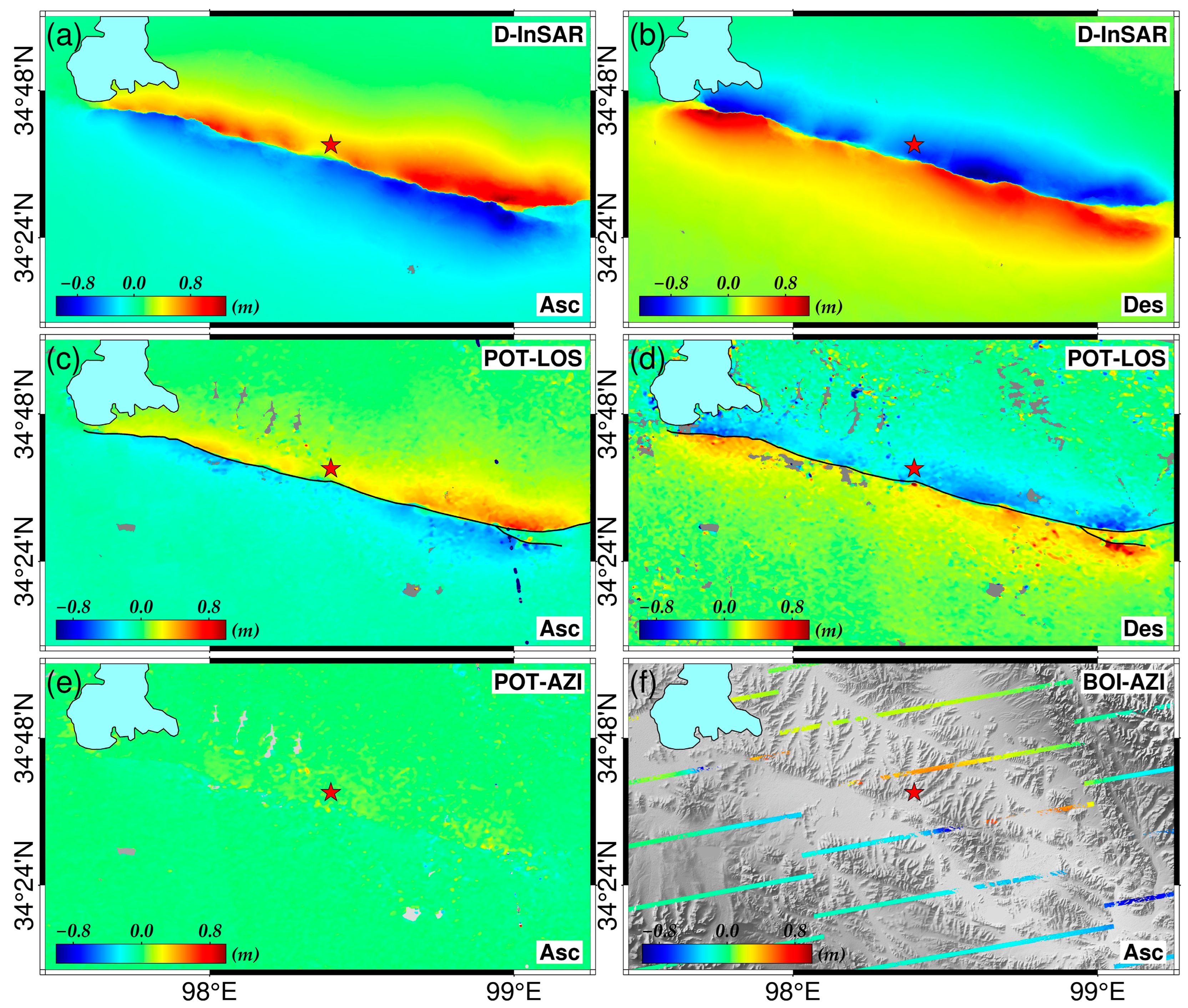
2.1. Coseismic Geodetic Observations
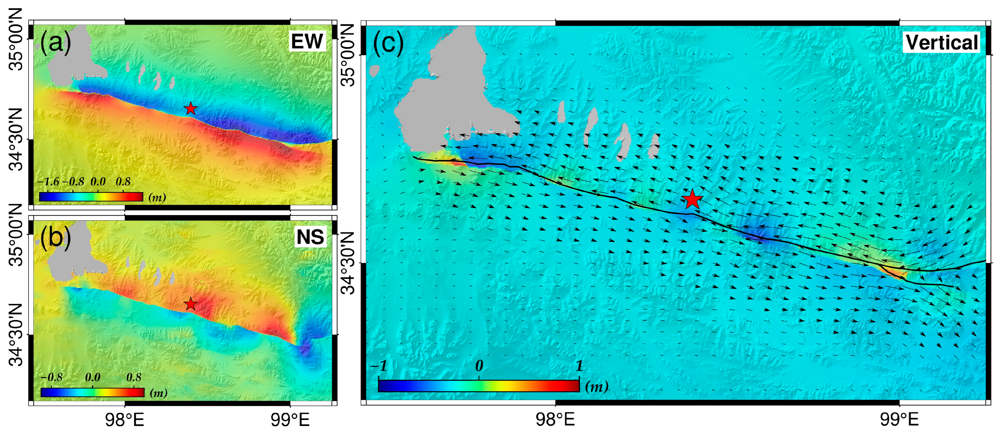
2.2. Three-Dimensional (3-D) Coseismic Deformation Field
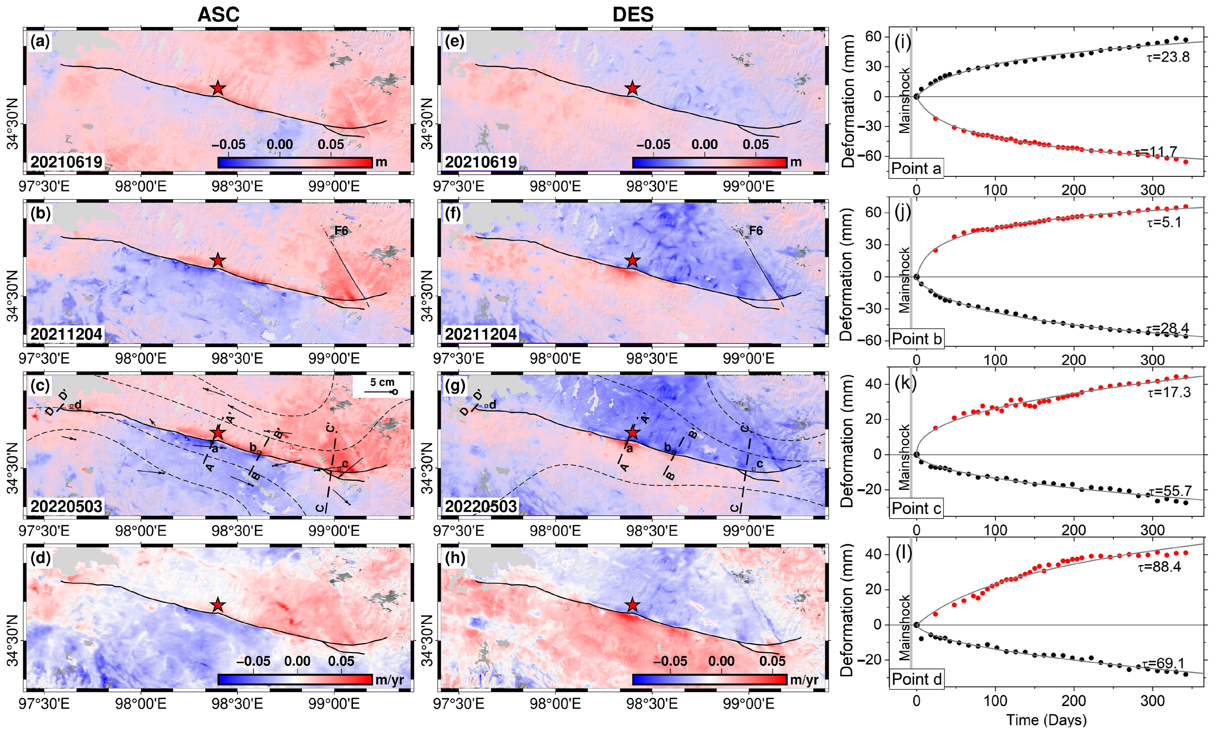
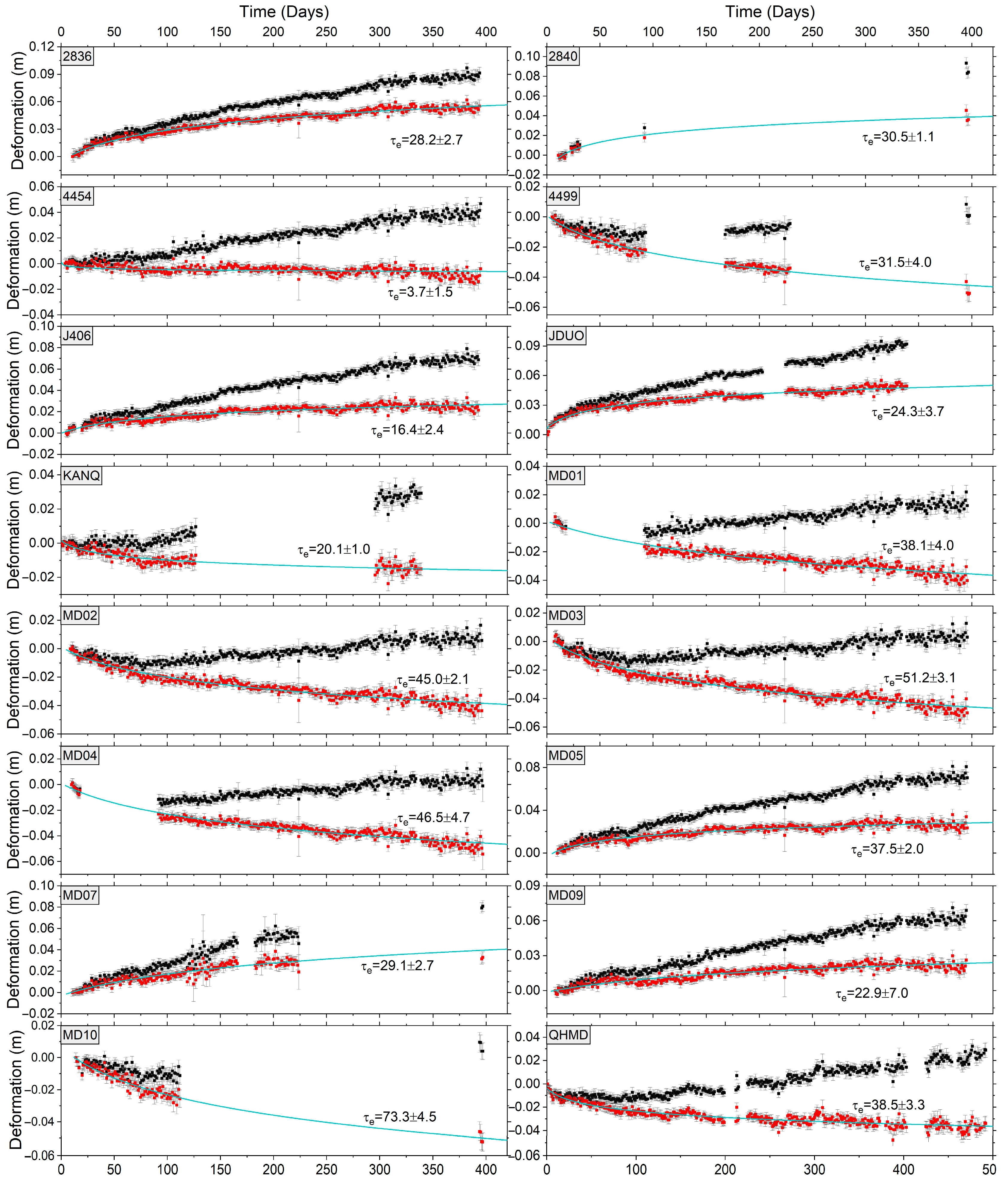
2.3. Postseismic Geodetic Observations
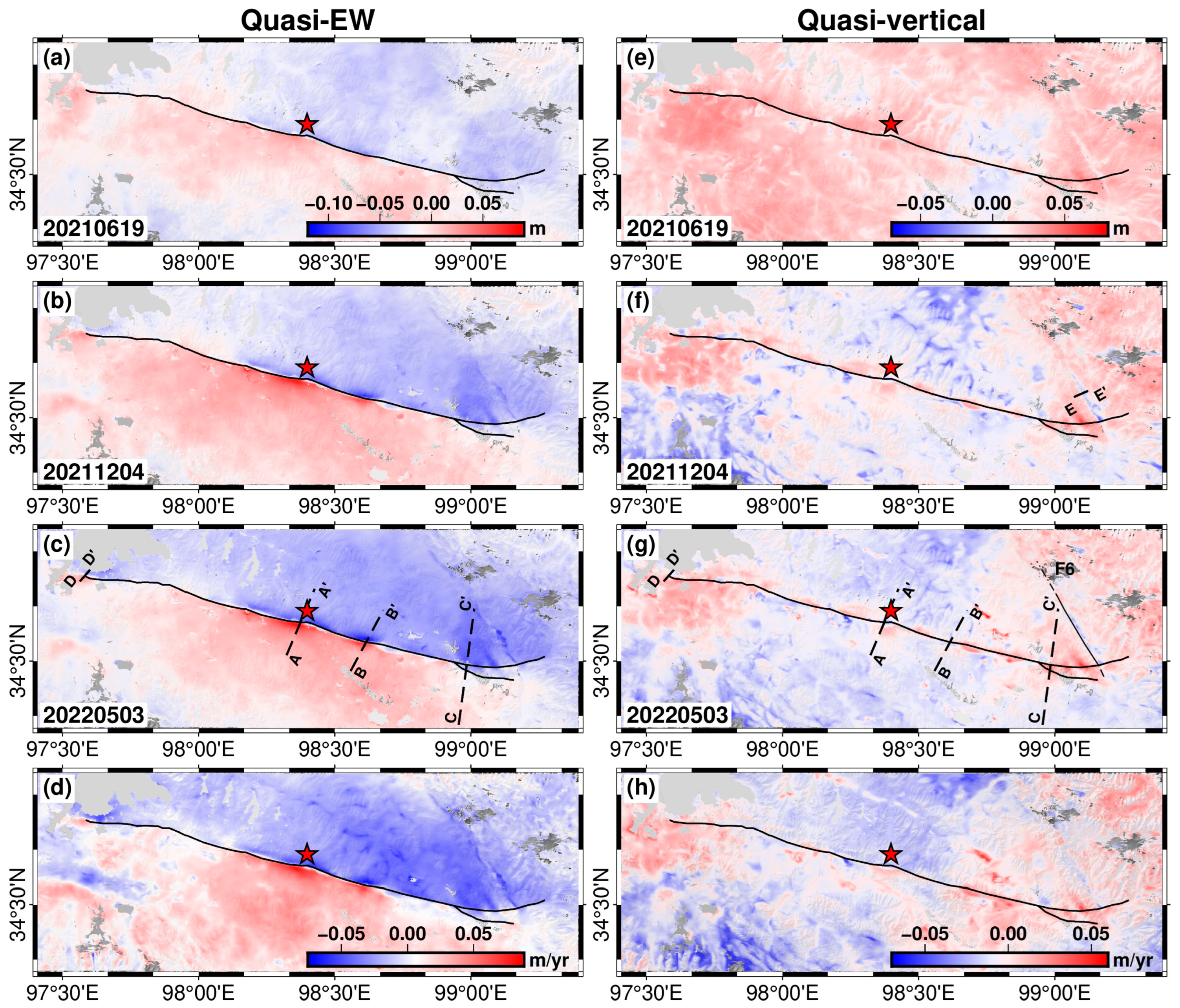
2.4. 2.5-Dimensional (2.5-D) Postseismic Time Series Deformation Decomposing
2.5. Co- and Postseismic Slip Modeling
2.6. Modeling of Viscoelastic Relaxation and Poroelastic Rebound
2.7. The Coulomb Failure Stress Change
3. Results and Analyses
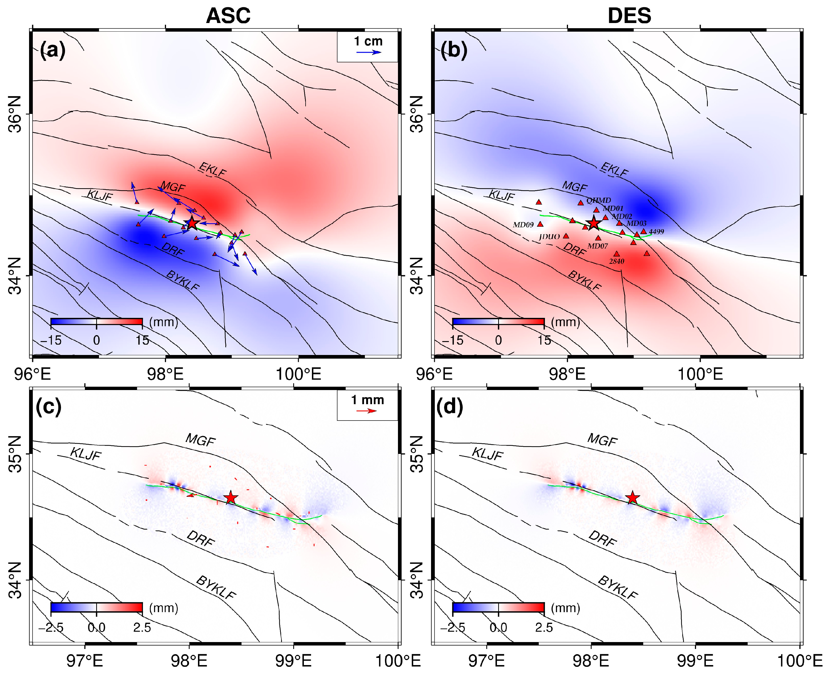
3.1. The Coseismic Deformation Analysis
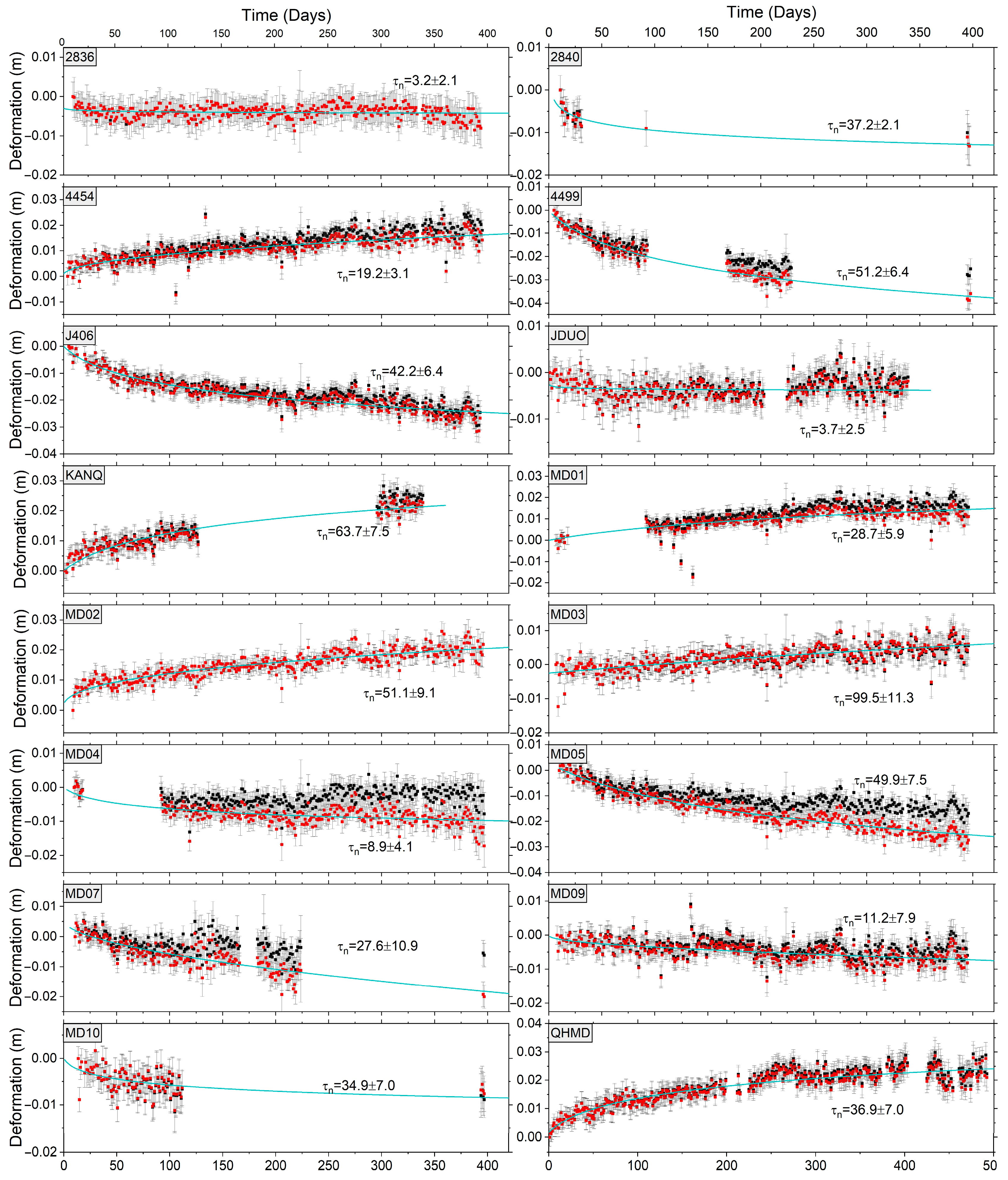
3.2. The Postseismic Deformation Analysis
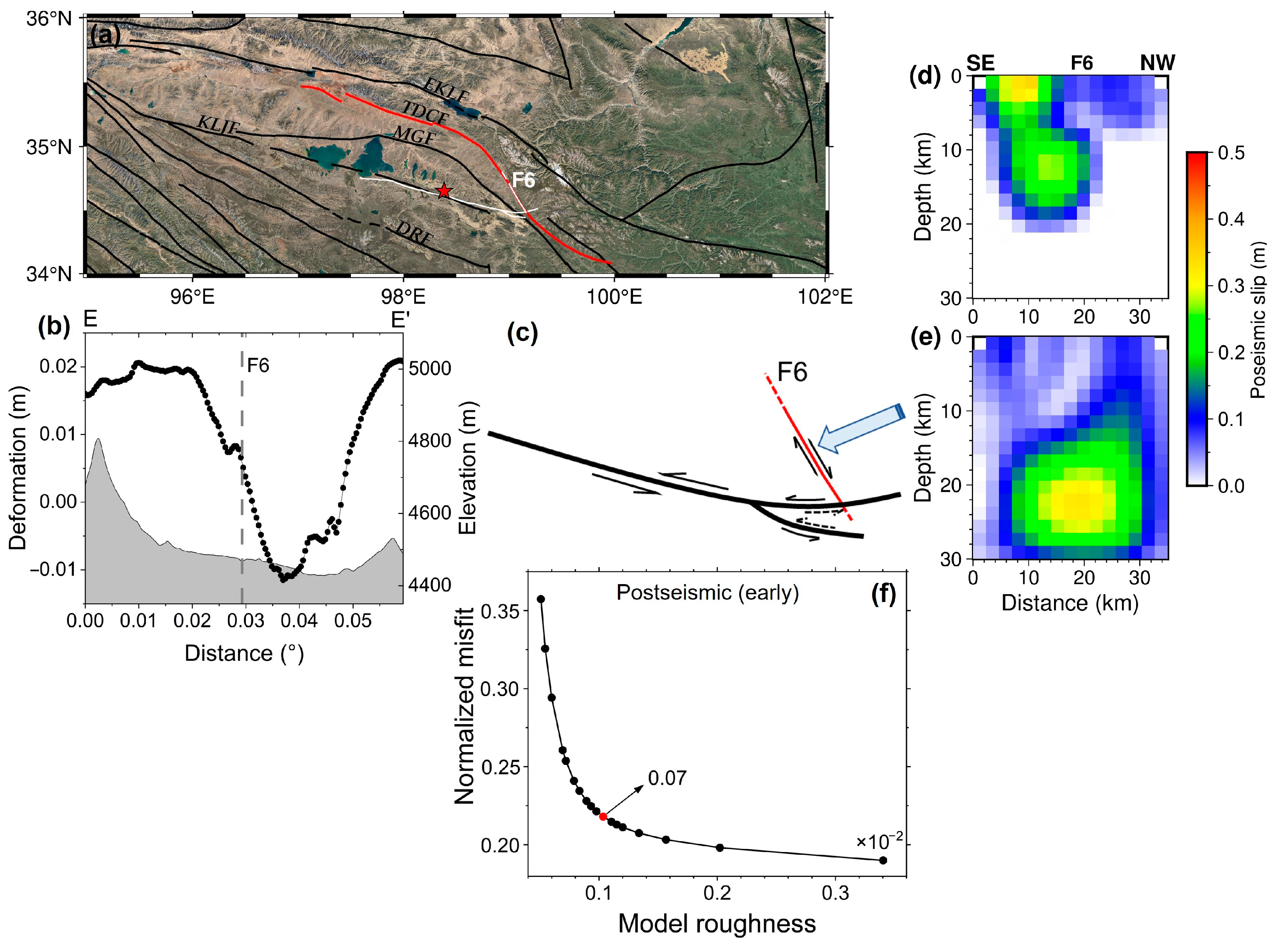
3.3. The Co- and Postseismic Slip Distribution
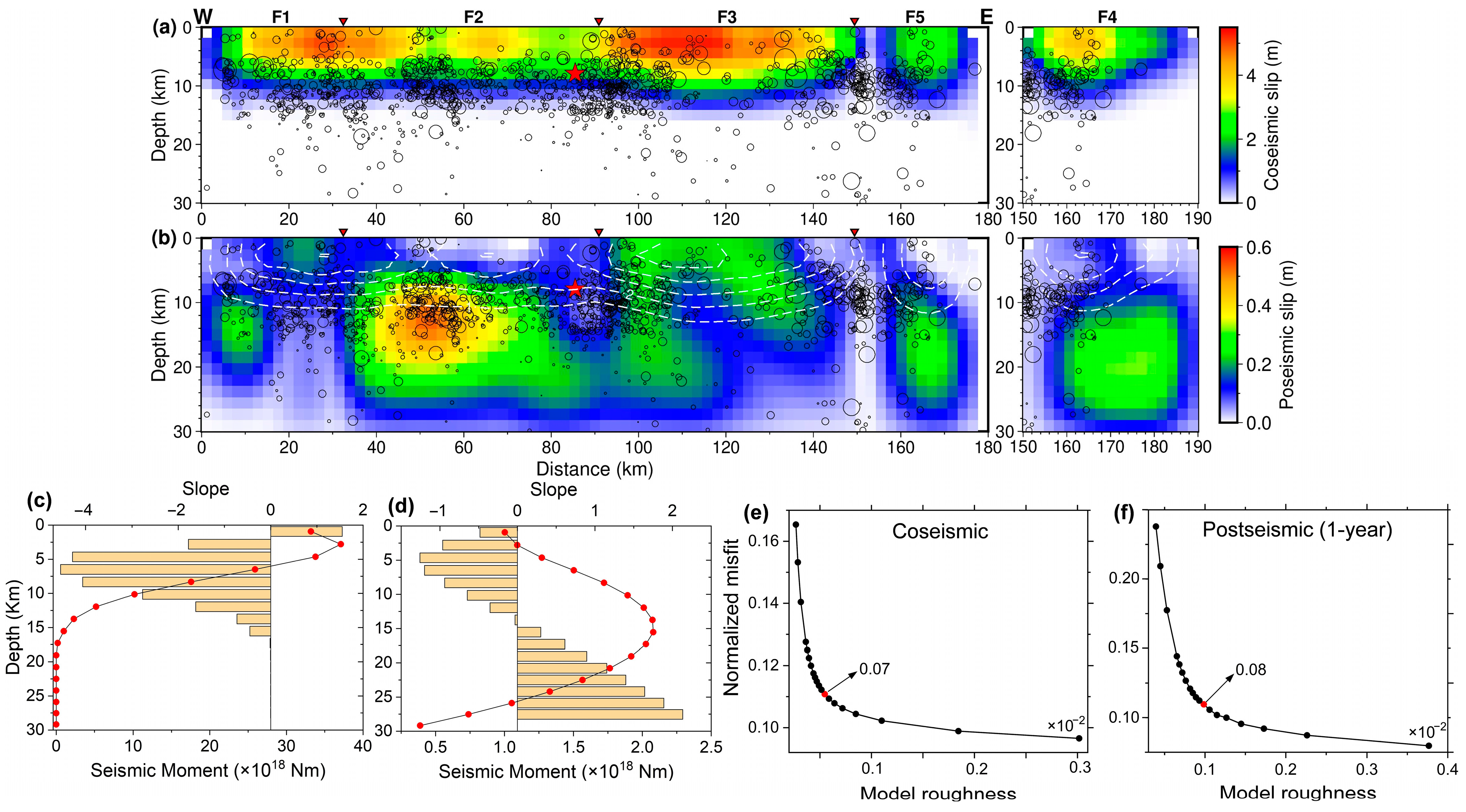
3.3.1. The Coseismic Slip Distribution
3.3.2. The Postseismic Slip Distribution
4. Discussion
4.1. Seismogenic Fault and Early Postseismic Mechanism
4.1.1. Early Postseismic Deformation Mechanism
4.1.2. Seismogenic Fault and Afterslip
4.1.3. Postseismic Seismic Moment Release Pattern
4.2. Existing Fault Reactivated
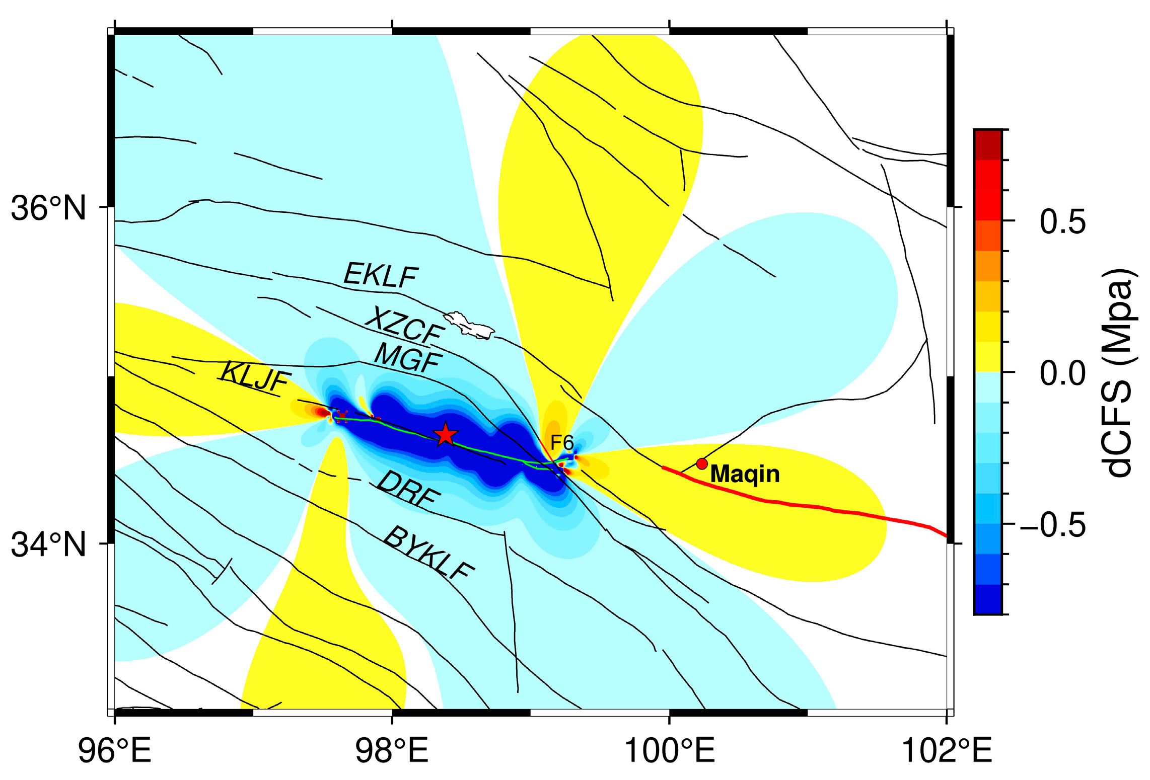
4.3. Potential Seismic Risks around the Maduo Event
5. Conclusions
- (1)
- Postseismic deformation can be explained by a combination of aseismic afterslip (near-field) and VR effect (near- and far-field). The contribution of PR to the postseismic deformation can be neglected;
- (2)
- The coseismic slip and postseismic afterslip exhibited a clear complementary and partially overlapping relationship. The overlapping area between coseismic slip and postseismic afterslip is likely driven by coseismic residual stress;
- (3)
- The Changmahe fault was reactivated by the Maduo event. The afterslip has continued to exert compression on it in the one year after the mainshock;
- (4)
- Stress analysis indicates that the seismic gaps in the Maqin-Maqu segment and the KLJF will be potential seismic risks in the future.
Supplementary Materials
Author Contributions
Funding
Data Availability Statement
Acknowledgments
Conflicts of Interest
Abbreviation
| SAR | Synthetic Aperture Radar |
| InSAR | Interferometric Synthetic Aperture Radar |
| D-InSAR | Two-pass differential InSAR |
| POT | Pixel offset tracking |
| BOI | Burst-Overlap Interferometry |
| LOS | Line-of-sight |
| SBAS-InSAR | Small baseline subset InSAR |
| EKLF | East Kunlun fault |
| KLJF | Kunlun Pass-Jiangcuo fault |
| DRF | Dari fault |
| MGF | Maduo-Gande fault |
| BYKLF | Bayan Har Mountain Main Peak fault |
| TDCF | Tibet Dagou-Changmahe fault |
| GACOS | General Atmospheric Correction Online Service |
| VR | Viscoelastic relaxation |
| PR | Poroelastic rebound |
| dCFS | Coulomb Failure stress change |
References
- Zhan, Y.; Liang, M.; Sun, X.; Huang, F.; Zhao, L.; Zhan, Y.; Gong, Y.; Han, J.; Li, C.; Zhang, P.; et al. Deep structure and seismogenic pattern of the 2021.5.22 Madoi (Qinghai) MS7.4 earthquake. Chin. J. Geophys. 2021, 64, 2232–2252. (In Chinese) [Google Scholar]
- Li, Z.; Li, W.; Li, T.; Xu, Y.; Su, P.; Guo, P.; Sun, H.; Ha, G.; Chen, G.; Yuan, Z. Seismogenic fault and coseismic surface deformation of the Maduo MS7.4 earthquake in Qinghai, China: A quick report. Seismol. Geol. 2021, 43, 722. [Google Scholar]
- Ren, J.; Xu, X.; Zhang, G.; Wang, Q.; Zhang, Z.; Gai, H.; Kang, W. Coseismic surface ruptures, slip distribution, and 3D seismogenic fault for the 2021 Mw 7.3 Maduo earthquake, central Tibetan Plateau, and its tectonic implications. Tectonophysics 2022, 827, 229275. [Google Scholar] [CrossRef]
- Wang, W.; Fang, L.; Wu, J.; Tu, H.; Chen, L.; Lai, G.; Zhang, L. Aftershock sequence relocation of the 2021 MS7.4 Maduo earthquake, Qinghai, China. Sci. China Earth Sci. 2021, 64, 1371–1380. [Google Scholar] [CrossRef]
- Wang, L.; Gao, H.; Feng, G.; Xu, W. Source parameters and triggering links of the earthquake sequence in central Italy from 2009 to 2016 analyzed with GPS and InSAR data. Tectonophysics 2018, 744, 285–295. [Google Scholar] [CrossRef]
- Wang, X.; Xu, C.; Xiao, Z.; Peng, Y. Source model for buried thrust-dominated earthquakes using partial InSAR displacements: The 2018 Lombok, Indonesia, earthquake sequence. Geophys. J. Int. 2022, 229, 1434–1447. [Google Scholar] [CrossRef]
- Xiong, W.; Chen, W.; Wang, D.; Wen, Y.; Nie, Z.; Liu, G.; Dijin, W.; Yu, P.; Qiao, X.; Zhao, B. Coseismic slip and early afterslip of the 2021 Mw 7.4 Maduo, China earthquake constrained by GPS and InSAR data. Tectonophysics 2022, 840, 229558. [Google Scholar] [CrossRef]
- Xu, G.; Xu, C.; Wen, Y.; Yin, Z. Coseismic and postseismic deformation of the 2016 MW 6.2 Lampa earthquake, southern Peru, constrained by interferometric synthetic aperture radar. J. Geophys. Res. Solid Earth 2019, 124, 4250–4272. [Google Scholar] [CrossRef]
- Fang, J.; Ou, Q.; Wright, T.J.; Okuwaki, R.; Amey, R.M.; Craig, T.J.; Elliott, J.R.; Hooper, A.; Lazecký, M.; Maghsoudi, Y. Earthquake Cycle Deformation Associated with the 2021 Mw 7.4 Maduo (Eastern Tibet) Earthquake: An Intrablock Rupture Event on a Slow-Slipping Fault from Sentinel-1 InSAR and Teleseismic Data. J. Geophys. Res. Solid Earth 2022, 127, e2022JB024268. [Google Scholar] [CrossRef]
- He, L.; Feng, G.; Wu, X.; Lu, H.; Xu, W.; Wang, Y.; Liu, J.; Hu, J.; Li, Z. Coseismic and early postseismic slip models of the 2021 Mw 7.4 Maduo earthquake (western China) estimated by space-based geodetic data. Geophys. Res. Lett. 2021, 48, e2021GL095860. [Google Scholar] [CrossRef]
- Lyu, M.; Chen, K.; Xue, C.; Zang, N.; Zhang, W.; Wei, G. Overall subshear but locally supershear rupture of the 2021 Mw 7.4 Maduo earthquake from high-rate GNSS waveforms and three-dimensional InSAR deformation. Tectonophysics 2022, 839, 229542. [Google Scholar] [CrossRef]
- Zhang, X.; Feng, W.; Du, H.; Samsonov, S.; Yi, L. Supershear rupture during the 2021 MW 7.4 Maduo, China, earthquake. Geophys. Res. Lett. 2022, 49, e2022GL097984. [Google Scholar] [CrossRef]
- Zhao, D.; Qu, C.; Chen, H.; Shan, X.; Song, X.; Gong, W. Tectonic and geometric control on fault kinematics of the 2021 Mw7.3 Maduo (China) earthquake inferred from interseismic, coseismic, and postseismic InSAR observations. Geophys. Res. Lett. 2021, 48, e2021GL095417. [Google Scholar] [CrossRef]
- Pan, J.; Bai, M.; Li, C.; Liu, F.; Li, H.; Liu, D.; Chevalier, M.; Wu, K.; Wang, P.; Lu, H. Coseismic surface rupture and seismogenic structure of the 2021-05-22 Maduo (Qinghai) MS 7.4 earthquake. Acta Geol. Sin. 2021, 95, 1655–1670. [Google Scholar]
- Yuan, Z.; Li, T.; Su, P.; Sun, H.; Ha, G.; Guo, P.; Chen, G.; Thompson Jobe, J. Large surface-rupture gaps and low surface fault slip of the 2021 Mw 7.4 Maduo earthquake along a low-activity strike-slip fault, Tibetan Plateau. Geophys. Res. Lett. 2022, 49, e2021GL096874. [Google Scholar]
- Yang, Y.; Xu, Q.; Hu, J.; Wang, Y.; Dong, X.; Chen, Q.; Zhang, Y.; Li, H. Source Model and Triggered Aseismic Faulting of the 2021 Mw 7.3 Maduo Earthquake Revealed by the UAV-Lidar/Photogrammetry, InSAR, and Field Investigation. Remote Sens. 2022, 14, 5859. [Google Scholar] [CrossRef]
- Zhao, L.; Xu, W.; Fang, N.; Liu, J.; Feng, G. Coseismic and early postseismic fault slip model and the seismogenic fault friction properties of the 2021 Qinghai Madoi MW7.3 earthquake. Chin. J. Geophys. 2023, 66, 1086–1097. (In Chinese) [Google Scholar]
- Jin, Z.; Fialko, Y.; Yang, H.; Li, Y. Transient deformation excited by the 2021 M7. 4 Maduo (China) earthquake: Evidence of a deep shear zone. J. Geophys. Res. Solid Earth 2023, 128, e2023JB026643. [Google Scholar] [CrossRef]
- Wei, S.; Zeng, H.; Shi, Q.; Liu, J.; Luo, H.; Hu, W.; Li, Y.; Wang, W.; Ma, Z.; Liu-Zeng, J. Simultaneous rupture propagation through fault bifurcation of the 2021 Mw7.4 Maduo earthquake. Geophys. Res. Lett. 2022, 49, e2022GL100283. [Google Scholar] [CrossRef]
- Deng, Q. Active tectonics and earthquake activities in China. Earth Sci. Front. 2003, 10, 66. (In Chinese) [Google Scholar]
- Qu, C. Building to the active tectonic database of China. Seismol. Geol. 2008, 30, 298–304. [Google Scholar]
- Diao, F.; Xiong, X.; Wang, R.; Walter, T.R.; Wang, Y.; Wang, K. Slip rate variation along the Kunlun fault (Tibet): Results from new GPS observations and a viscoelastic earthquake-cycle deformation model. Geophys. Res. Lett. 2019, 46, 2524–2533. [Google Scholar] [CrossRef]
- Wang, M.; Shen, Z.K. Present-day crustal deformation of continental China derived from GPS and its tectonic implications. J. Geophys. Res. Solid Earth 2020, 125, e2019JB018774. [Google Scholar] [CrossRef]
- Molnar, P.; Deng, Q. Faulting associated with large earthquakes and the average rate of deformation in central and eastern Asia. J. Geophys. Res. Solid Earth 1984, 89, 6203–6227. [Google Scholar] [CrossRef]
- Rosen, P.A.; Gurrola, E.; Sacco, G.F.; Zebker, H. The InSAR Scientific Computing Environment. In Proceedings of the EUSAR 2012: 9th European Conference on Synthetic Aperture Radar, Nuremberg, Germany, 23–26 April 2012; VDE: Berlin, Germany, 2012; pp. 730–733. [Google Scholar]
- Goldstein, R.M.; Werner, C.L. Radar interferogram filtering for geophysical applications. Geophys. Res. Lett. 1998, 25, 4035–4038. [Google Scholar] [CrossRef]
- Yu, C.; Li, Z.; Penna, N.T.; Crippa, P. Generic atmospheric correction model for interferometric synthetic aperture radar observations. J. Geophys. Res. Solid Earth 2018, 123, 9202–9222. [Google Scholar] [CrossRef]
- Pepe, A.; Lanari, R. On the extension of the minimum cost flow algorithm for phase unwrapping of multitemporal differential SAR interferograms. IEEE Trans. Geosci. Remote Sens. 2006, 44, 2374–2383. [Google Scholar] [CrossRef]
- Gray, A.; Short, N.; Mattar, K.; Jezek, K. Velocities and flux of the Filchner Ice Shelf and its tributaries determined from speckle tracking interferometry. Can. J. Remote Sens. 2001, 27, 193–206. [Google Scholar] [CrossRef]
- Rott, H.; Stuefer, M.; Siegel, A.; Skvarca, P.; Eckstaller, A. Mass fluxes and dynamics of Moreno glacier, southern Patagonia icefield. Geophys. Res. Lett. 1998, 25, 1407–1410. [Google Scholar] [CrossRef]
- Solaro, G.; De Novellis, V.; Castaldo, R.; De Luca, C.; Lanari, R.; Manunta, M.; Casu, F. Coseismic fault model of Mw 8.3 2015 Illapel earthquake (Chile) retrieved from multi-orbit Sentinel1-A DInSAR measurements. Remote Sens. 2016, 8, 323. [Google Scholar] [CrossRef]
- Hu, J.; Liu, J.; Li, Z.; Zhu, J.; Wu, L.; Sun, Q.; Wu, W. Estimating three-dimensional coseismic deformations with the SM-VCE method based on heterogeneous SAR observations: Selection of homogeneous points and analysis of observation combinations. Remote Sens. Environ. 2021, 255, 112298. [Google Scholar] [CrossRef]
- Liu, J.; Hu, J.; Li, Z.; Zhu, J.; Sun, Q.; Gan, J. A method for measuring 3-D surface deformations with InSAR based on strain model and variance component estimation. IEEE Trans. Geosci. Remote Sens. 2017, 56, 239–250. [Google Scholar] [CrossRef]
- Agram, P.; Jolivet, R.; Riel, B.; Lin, Y.; Simons, M.; Hetland, E.; Doin, M.P.; Lasserre, C. New radar interferometric time series analysis toolbox released. Eos Trans. Am. Geophys. Union 2013, 94, 69–70. [Google Scholar] [CrossRef]
- Hooper, A. A multi-temporal InSAR method incorporating both persistent scatterer and small baseline approaches. Geophys. Res. Lett. 2008, 35. [Google Scholar] [CrossRef]
- Berardino, P.; Fornaro, G.; Lanari, R.; Sansosti, E. A new algorithm for surface deformation monitoring based on small baseline differential SAR interferograms. IEEE Trans. Geosci. Remote Sens. 2002, 40, 2375–2383. [Google Scholar] [CrossRef]
- Sandwell, D.T.; Price, E.J. Phase gradient approach to stacking interferograms. J. Geophys. Res. Solid Earth 1998, 103, 30183–30204. [Google Scholar] [CrossRef]
- Yue, H.; Sun, J.; Wang, M.; Shen, Z.; Li, M.; Xue, L.; Lu, W.; Zhou, Y.; Ren, C.; Lay, T. The 2019 Ridgecrest, California earthquake sequence: Evolution of seismic and aseismic slip on an orthogonal fault system. Earth Planet. Sci. Lett. 2021, 570, 117066. [Google Scholar] [CrossRef]
- Chen, C.W.; Zebker, H.A. Phase unwrapping for large SAR interferograms: Statistical segmentation and generalized network models. IEEE Trans. Geosci. Remote Sens. 2002, 40, 1709–1719. [Google Scholar] [CrossRef]
- Hong, S.; Liu, M. Postseismic deformation and afterslip evolution of the 2015 Gorkha earthquake constrained by InSAR and GPS observations. J. Geophys. Res. Solid Earth 2021, 126, e2020JB020230. [Google Scholar]
- Fujiwara, S.; Nishimura, T.; Murakami, M.; Nakagawa, H.; Tobita, M.; Rosen, P.A. 2.5-D surface deformation of M6.1 earthquake near Mt Iwate detected by SAR interferometry. Geophys. Res. Lett. 2000, 27, 2049–2052. [Google Scholar] [CrossRef]
- Wang, R.; Parolai, S.; Ge, M.; Jin, M.; Walter, T.R.; Zschau, J. The 2011 Mw 9.0 Tohoku earthquake: Comparison of GPS and strong-motion data. Bull. Seismol. Soc. Am. 2013, 103, 1336–1347. [Google Scholar] [CrossRef]
- Chen, Y.; Hu, Y.; Qian, L.; Meng, G. Early postseismic deformation of the 2010 Mw 6.9 Yushu earthquake and its implication for lithospheric rheological properties. Geophys. Res. Lett. 2022, 49, e2022GL098942. [Google Scholar] [CrossRef]
- Peña, C.; Metzger, S.; Heidbach, O.; Bedford, J.; Bookhagen, B.; Moreno, M.; Oncken, O.; Cotton, F. Role of poroelasticity during the early postseismic deformation of the 2010 Maule megathrust earthquake. Geophys. Res. Lett. 2022, 49, e2022GL098144. [Google Scholar]
- Bürgmann, R.; Dresen, G. Rheology of the lower crust and upper mantle: Evidence from rock mechanics, geodesy, and field observations. Annu. Rev. Earth Planet. Sci. 2008, 36, 531–567. [Google Scholar] [CrossRef]
- Wang, R.; Lorenzo-Martín, F.; Roth, F. PSGRN/PSCMP—A new code for calculating co-and post-seismic deformation, geoid and gravity changes based on the viscoelastic-gravitational dislocation theory. Comput. Geosci. 2006, 32, 527–541. [Google Scholar] [CrossRef]
- Song, X.; Wang, S.; Pan, S.; Song, J. Deep seismotectonic environment of the 2021 Madoi Ms7.4 earthquake. Seismol. Geol. 2021, 43, 757–770. [Google Scholar]
- Liu, L.; Li, Y.; Zhu, L.; Ji, L. Influence of the 1947 Dari M7.7 earthquake on stress evolution along the boundary fault of the Bayan Har block: Insights from numerical simulation. Chin. J. Geophys. 2021, 64, 2221–2231. (In Chinese) [Google Scholar]
- Peltzer, G.; Rosen, P.; Rogez, F.; Hudnut, K. Poroelastic rebound along the Landers 1992 earthquake surface rupture. J. Geophys. Res. Solid Earth 1998, 103, 30131–30145. [Google Scholar] [CrossRef]
- Wang, R.; Kümpel, H.-J. Poroelasticity: Efficient modeling of strongly coupled, slow deformation processes in a multilayered half-space. Geophysics 2003, 68, 705–717. [Google Scholar] [CrossRef]
- Chen, H.; Qu, C.; Zhao, D.; Ma, C.; Shan, X. Rupture kinematics and coseismic slip model of the 2021 Mw 7.3 Maduo (China) earthquake: Implications for the seismic hazard of the Kunlun fault. Remote Sens. 2021, 13, 3327. [Google Scholar] [CrossRef]
- Hong, S.; Liu, M.; Liu, T.; Dong, Y.; Chen, L.; Meng, G.; Xu, Y. Fault Source Model and Stress Changes of the 2021 Mw 7.4 Maduo Earthquake, China, Constrained by InSAR and GPS Measurements. Bull. Seismol. Soc. Am. 2022, 112, 1284–1296. [Google Scholar] [CrossRef]
- Liu, J.; Hu, J.; Li, Z.; Ma, Z.; Wu, L.; Jiang, W.; Feng, G.; Zhu, J. Complete three-dimensional coseismic displacements due to the 2021 Maduo earthquake in Qinghai Province, China from Sentinel-1 and ALOS-2 SAR images. Sci. China Earth Sci. 2022, 65, 687–697. [Google Scholar] [CrossRef]
- Gonzalez-Ortega, A.; Fialko, Y.; Sandwell, D.; Alejandro Nava-Pichardo, F.; Fletcher, J.; Gonzalez-Garcia, J.; Lipovsky, B.; Floyd, M.; Funning, G. El Mayor-Cucapah (Mw 7.2) earthquake: Early near-field postseismic deformation from InSAR and GPS observations. J. Geophys. Res. Solid Earth 2014, 119, 1482–1497. [Google Scholar] [CrossRef]
- Tang, X.; Guo, R.; Xu, J.; Zheng, Y. Role of Poroelasticity and Viscoelasticity during the Postseismic Deformation of the 2021 Mw 7.4 Maduo, China, Earthquake. Seismol. Res. Lett. 2023, 94, 2192–2201. [Google Scholar] [CrossRef]
- Yue, H.; Shen, Z.-K.; Zhao, Z.; Wang, T.; Cao, B.; Li, Z.; Bao, X.; Zhao, L.; Song, X.; Ge, Z. Rupture process of the 2021 M7.4 Maduo earthquake and implication for deformation mode of the Songpan-Ganzi terrane in Tibetan Plateau. Proc. Natl. Acad. Sci. USA 2022, 119, e2116445119. [Google Scholar] [CrossRef] [PubMed]
- Jin, Z.; Fialko, Y. Coseismic and early postseismic deformation due to the 2021 M7.4 Maduo (China) earthquake. Geophys. Res. Lett. 2021, 48, e2021GL095213. [Google Scholar] [CrossRef]
- Dianala, J.D.B.; Jolivet, R.; Thomas, M.Y.; Fukushima, Y.; Parsons, B.; Walker, R. The relationship between seismic and aseismic slip on the Philippine Fault on Leyte Island: Bayesian modeling of fault slip and geothermal subsidence. J. Geophys. Res. Solid Earth 2020, 125, e2020JB020052. [Google Scholar] [CrossRef]
- Dieterich, J.H. Earthquake nucleation on faults with rate-and state-dependent strength. Tectonophysics 1992, 211, 115–134. [Google Scholar] [CrossRef]
- Marone, C. Laboratory-derived friction laws and their application to seismic faulting. Annu. Rev. Earth Planet. Sci. 1998, 26, 643–696. [Google Scholar] [CrossRef]
- Marone, C.J.; Scholtz, C.; Bilham, R. On the mechanics of earthquake afterslip. J. Geophys. Res. Solid Earth 1991, 96, 8441–8452. [Google Scholar] [CrossRef]
- Bedford, J.; Moreno, M.; Baez, J.C.; Lange, D.; Tilmann, F.; Rosenau, M.; Heidbach, O.; Oncken, O.; Bartsch, M.; Rietbrock, A. A high-resolution, time-variable afterslip model for the 2010 Maule Mw = 8.8, Chile megathrust earthquake. Earth Planet. Sci. Lett. 2013, 383, 26–36. [Google Scholar] [CrossRef]
- Iinuma, T.; Hino, R.; Uchida, N.; Nakamura, W.; Kido, M.; Osada, Y.; Miura, S. Seafloor observations indicate spatial separation of coseismic and postseismic slips in the 2011 Tohoku earthquake. Nat. Commun. 2016, 7, 13506. [Google Scholar] [CrossRef]
- Liu, X.; Xu, W. Logarithmic model joint inversion method for coseismic and postseismic slip: Application to the 2017 Mw 7.3 Sarpol Zahāb earthquake, Iran. J. Geophys. Res. Solid Earth 2019, 124, 12034–12052. [Google Scholar] [CrossRef]
- Yabe, S.; Ide, S. Why do aftershocks occur within the rupture area of a large earthquake? Geophys. Res. Lett. 2018, 45, 4780–4787. [Google Scholar] [CrossRef]
- Zhao, B.; Bürgmann, R.; Wang, D.; Tan, K.; Du, R.; Zhang, R. Dominant controls of downdip afterslip and viscous relaxation on the postseismic displacements following the Mw7.9 Gorkha, Nepal, earthquake. J. Geophys. Res. Solid Earth 2017, 122, 8376–8401. [Google Scholar] [CrossRef]
- Pan, J.; Li, H.; Chevalier, M.-L.; Tapponnier, P.; Bai, M.; Li, C.; Liu, F.; Liu, D.; Wu, K.; Wang, P. Co-seismic rupture of the 2021, Mw7.4 Maduo earthquake (northern Tibet): Short-cutting of the Kunlun fault big bend. Earth Planet. Sci. Lett. 2022, 594, 117703. [Google Scholar] [CrossRef]
- Hua, J.; Zhao, D.; Shan, X.; Qu, C.; Zhang, Y.; Gong, W.; Wang, Z.; Li, C.; Zhao, L.; Li, Y.; et al. Coseismic deformation field, slip distribution and Coulomb stress disturbance of the 2021 MW7.3 Maduo earthquake using sentinel-1 InSAR observations. Seismol. Geol. 2021, 43, 677–691. [Google Scholar]
- Zhu, L.; Ji, L.; Liu, C. Interseismic slip rate and locking along the Maqin–Maqu Segment of the East Kunlun Fault, Northern Tibetan Plateau, based on Sentinel-1 images. J. Asian Earth Sci. 2021, 211, 104703. [Google Scholar] [CrossRef]
- Ha, G.; Liu, J.; Ren, Z.; Zhu, X.; Bao, G.; Wu, D.; Zhang, Z. The Interpretation of Seismogenic Fault of the Maduo Mw 7.3 Earthquake, Qinghai Based on Remote Sensing Images—A Branch of the East Kunlun Fault System. J. Earth Sci. 2022, 33, 857–868. [Google Scholar] [CrossRef]
- Wang, M.; Shen, Z.K.; Wang, Y.Z.; Bürgmann, R.; Wang, F.; Zhang, P.Z.; Liao, H.; Zhang, R.; Wang, Q.; Jiang, Z.S. Postseismic deformation of the 2008 Wenchuan earthquake illuminates lithospheric rheological structure and dynamics of eastern Tibet. J. Geophys. Res. Solid Earth 2021, 126, e2021JB022399. [Google Scholar] [CrossRef]
- Wessel, P.; Smith, W.H.; Scharroo, R.; Luis, J.; Wobbe, F. Generic mapping tools: Improved version released. Eos Trans. Am. Geophys. Union 2013, 94, 409–410. [Google Scholar] [CrossRef]


| Site | EGPS (cm) | SigE (mm) | EInSAR (cm) | SigE (mm) | NGPS (cm) | SigN (mm) | NInSAR (cm) | SigN (mm) |
|---|---|---|---|---|---|---|---|---|
| 4441 | −13.663 | 3.393 | −11.263 | 9.572 | 16.55 | 3.691 | 16.89 | 8.323 |
| 4495 | −29.187 | 1.013 | −24.394 | 2.077 | −12.321 | 1.087 | −7.471 | 3.401 |
| 4499 | −102.307 | 0.845 | −101.316 | 14.54 | −49.836 | 1.309 | −49.962 | 9.935 |
| J005 | −27.506 | 1.221 | −24.943 | 2.714 | 10.129 | 1.421 | 5.618 | 2.358 |
| J406 | 22.444 | 1.516 | 20.789 | 2.06 | −26.277 | 1.182 | −22.875 | 1.79 |
| JDUO | 27.81 | 0.754 | 28.478 | 3.275 | −5.37 | 0.909 | −5.81 | 2.846 |
| MADU | −23.618 | 0.893 | −21.455 | 4.648 | 8.971 | 0.461 | 5.189 | 4.04 |
| QHAH | 13.625 | 6.31 | 14.644 | 2.123 | −1.483 | 7.79 | −0.405 | 1.845 |
| QHAJ | −47.154 | 4.12 | −46.092 | 3.746 | −30.186 | 5.35 | −28.346 | 3.254 |
| RMSE (cm) | 2.2685 | 2.8795 | ||||||
Disclaimer/Publisher’s Note: The statements, opinions and data contained in all publications are solely those of the individual author(s) and contributor(s) and not of MDPI and/or the editor(s). MDPI and/or the editor(s) disclaim responsibility for any injury to people or property resulting from any ideas, methods, instructions or products referred to in the content. |
© 2024 by the authors. Licensee MDPI, Basel, Switzerland. This article is an open access article distributed under the terms and conditions of the Creative Commons Attribution (CC BY) license (https://creativecommons.org/licenses/by/4.0/).
Share and Cite
Shu, C.; Meng, Z.; Wu, Q.; Xiong, W.; He, L.; Zhang, X.; Xu, D. Coseismic and Early Postseismic Deformation Mechanism Following the 2021 Mw 7.4 Maduo Earthquake: Insights from Satellite Radar Interferometry and GPS. Remote Sens. 2024, 16, 1399. https://doi.org/10.3390/rs16081399
Shu C, Meng Z, Wu Q, Xiong W, He L, Zhang X, Xu D. Coseismic and Early Postseismic Deformation Mechanism Following the 2021 Mw 7.4 Maduo Earthquake: Insights from Satellite Radar Interferometry and GPS. Remote Sensing. 2024; 16(8):1399. https://doi.org/10.3390/rs16081399
Chicago/Turabian StyleShu, Chuanzeng, Zhiguo Meng, Qiong Wu, Wei Xiong, Lijia He, Xiaoping Zhang, and Dan Xu. 2024. "Coseismic and Early Postseismic Deformation Mechanism Following the 2021 Mw 7.4 Maduo Earthquake: Insights from Satellite Radar Interferometry and GPS" Remote Sensing 16, no. 8: 1399. https://doi.org/10.3390/rs16081399