Early Prediction of Regional Red Needle Cast Outbreaks Using Climatic Data Trends and Satellite-Derived Observations

Abstract

Red needle cast (RNC), mainly caused by Phytophthora pluvialis, is a very damaging disease of the widely grown species radiata pine within New Zealand. Using a combination of satellite imagery and weather data, a novel methodology was developed to pre-visually predict the incidence of RNC on radiata pine within the Gisborne region of New Zealand over a five-year period from 2019 to 2023. Sentinel-2 satellite imagery was used to classify areas within the region as being disease-free or showing RNC expression from the difference in the red/green index (R/G_diff) during a disease-free time of the year and the time of maximum disease expression in the upper canopy (early spring–September). Within these two classes, 1976 plots were extracted, and a classification model was used to predict disease incidence from mean monthly weather data for key variables during the 11 months prior to disease expression. The variables in the final random forest model included solar radiation, relative humidity, rainfall, and the maximum air temperature recorded during mid–late summer, which provided a pre-visual prediction of the disease 7–8 months before its peak expression. Using a hold-out test dataset, the final random forest model had an accuracy of 89% and an F1 score of 0.89. This approach can be used to mitigate the impact of RNC by focusing on early surveillance and treatment measures.

1. Introduction

Radiata pine (Pinus radiata D. Don) is the most extensively planted conifer globally and constitutes the cornerstone of New Zealand’s forest industry, comprising 90% of the 1.8 M ha plantation resource [1]. Radiata pine is vulnerable to several damaging diseases, with red needle cast (RNC) emerging as a significant threat to the species over the past fifteen years. This disease is primarily caused by the oomycete pathogen Phytophthora pluvialis and occasionally by Phytophthora kernoviae [2]. The symptoms of RNC have been observed since at least 2005, with confirmation of Phytophthora infection in 2008 [2]. Since then, RNC has spread extensively and now affects most areas in the North Island and many regions in the South Island. However, most damage from the disease has been reported from central and north-eastern regions of the North Island [3].

Outbreaks of RNC by P. pluvialis are restricted to the needle tissue on radiata pine and appear to be polycyclic [2]. Following infection, P. pluvialis establishes within the needle as mycelium before producing semi-caducous sporangia through the stomata within three days under optimal laboratory conditions [4]. Sporangia may germinate directly or through the production of zoospores, which are spread locally by water splash to initiate new infections on the same needle or nearby needles [4]. This infection cycle can continue to repeat whilst conditions remain favorable and susceptible host tissue is present. Both pathogens are also capable of producing oospores, which are typically longer-lived spores and are believed to have a role in the survival of Phytophthora between epidemics; however, P. pluvialis oospores have only been observed in vitro to date. Phytophthora pluvialis symptoms typically form during or following sporulation [2]. Initial symptoms of the disease are characterized by dark green lesions, frequently accompanied by narrow, dark, resinous bands. These lesions rapidly transition to a khaki hue, subsequently turning yellow or red, which precedes the abscission of entire fascicles [2].

The timing of symptom expression varies across sites and between years. Typically, symptoms on diseased trees emerge during late autumn or winter months and are initiated on the lower branches and progressively spread upwards through the crown and to adjacent trees, with the crown changing from green to red-brown and then brown (Figure 1). By early spring, needle loss can be extensive and, in severe cases, results in near-complete defoliation [2]. As current spring growth is seldom affected by the disease, trees often appear to have recovered by summer, with their crowns returning to a green color, although with a reduced crown density. However, the impact of needle loss due to RNC on radiata pine growth is significant. The stem basal area growth is found to be reduced by as much as 35% in the year following severe disease [5].

Seasonal patterns of RNC expression are strongly driven by climate. Needle wetness is required for the infection and sporulation of P. pluvialis on radiata pine needles (McLay et al. unpub. data), and culture growth has upper limits of 25 °C [6]. Likewise, P. kernoviae is limited by warm temperatures with no infection above 22 °C [7]. Field studies investigating P. pluvialis and P. kernoviae sporulation and the infection of radiata pine also indicate that lower temperatures and sufficient rainfall are required for these processes [8,9]. This results in the seasonal patterns of disease in which higher expression is noted in cooler and wetter months, between mid-autumn and mid-spring, with reduced detection during the warmer and drier summer months [8,9]. There is some evidence that climate conditions over summer may be a key driver of RNC’s extent and severity during the following seasons. A summer drought in 2011–2012 corresponded with the reduced detection of P. pluvialis and P. kernoviae the following year, while milder and wetter summers were followed by a greater expression of the disease [8]. Summer conditions may influence the rate at which the infection cycle can repeat and, thus, the level of initial inoculum to start the next epidemic [9]. Despite the strong relationship between weather variables and RNC, models that predict disease expression using climate are yet to be published.

Outbreaks of RNC have been intermittent and uneven, with high among-site and between-year variation in the incidence and severity of symptoms, as well as the timing of expression. This variation can make decisions on investment into disease management difficult. For Dothistroma needle blight (Dothistroma septosporum), which is another important pine needle disease in New Zealand forests, with a long history of management, disease persists on sites across years, and severity can increase year on year. Chemical control is applied to symptomatic trees (from infections of the previous season) in spring to protect newly emerging needles and future growth [10]. The polycyclic nature of RNC and its ability to develop rapidly under conducive conditions, combined with its often seemingly sporadic development, means that new approaches to disease management are required. There is a critical need to monitor disease expression at this scale to quantify between-year variation and to determine the climatic drivers, potentially enabling disease prediction and pre-emptive disease control activities [11].

Multispectral satellite imagery has significant potential as a data source for the regional detection of outbreaks from damaging diseases such as RNC. Most studies in the remote sensing literature have used satellite imagery to characterize and monitor insect outbreaks [12,13,14,15], and despite the substantial global impact of forest pathogens [16,17], very few have used satellite imagery to detect disease. Using very high resolution (VHR) QuickBird imagery, the occurrence of pitch canker, which is caused by Fusarium circinatum, was mapped in a moderate-sized plantation of radiata pine in South Africa [18]. Similarly, VHR WorldView satellite imagery was used at two sites in north-eastern New Zealand to develop a classification model of RNC in radiata pine from the red/green/blue (RGB) and near-infrared bands [19]. Although these studies show that disease can be accurately mapped from satellite imagery, it is expensive to scale detections to the regional level using imagery from VHR satellites, which are not that suitable for continuous monitoring as they require tasking.

The European Space Agency’s Sentinel-2 satellites offer an attractive alternative for large-area monitoring. Sentinel-2 data are open-access and have a high enough spatial resolution for stand-level disease detection, while the wide swath width and relatively high revisit frequency is well suited to regional-scale mapping and monitoring activities. High resolution Sentinel-2 imagery has been used to accurately detect the decline of maritime pine (Pinus pinaster) from pinewood nematode within three relatively small test areas in central Portugal [20]. Although the potential of Sentinel-2 has been recognized and utilized for the broad scale mapping of forest species (Breidenbach et al., 2021), bark beetle outbreaks [21], and global land use cover [22], we are unaware of any studies that have used Sentinel-2 data for the regional monitoring and mapping of forest disease.

Although little research has successfully detected disease prior to expression, the pre-visual prediction of disease across large scales would be very useful as it allows managers to manage disease outbreaks more effectively. Hyperspectral and thermal imagery has often been used for the pre-visual detection of diseases at a range of scales. Physiological responses in plants subject to infection by pathogens often include changes in chlorophyll and other pigments, leaf water content, and key photosynthetic variables, such as stomatal conductance, transpiration, and photosynthesis. These changes may be detected by shifts in leaf temperature and changes in indices or plant functional traits [23]. Using these indices, hyperspectral and thermal imagery has been used to pre-visually detect a range of diseases in both agricultural and forestry crops [24,25,26,27,28,29]. However, hyperspectral and thermal imagery acquired from airborne sensors is very expensive and time consuming to process, particularly at large scales. While hyperspectral and thermal data from satellites cover wide spatial extents, this has not been widely used over large areas for pre-visual disease detection due to infrequent revisit times, cloud cover during revisit, and the high cost of data acquisition.

Although little research has investigated this approach, the use of weather data may provide a robust and low-cost method for the pre-visual prediction of disease at a broad spatial scale. Disease occurrence and severity are often the result of environmental conditions favorable for pathogen development that occur months before the disease is expressed. A number of studies have identified the conditions or thresholds that regulate the level of disease expression for discrete sites [30,31]. For instance, Dothistroma needle blight has been shown to be more severe in a range of pine species when rainfall is high during the preceding summer [32,33,34]. Despite the promise of this approach, very little research has predicted pre-visual spatial variations in disease at a broad scale using weather surfaces that characterize conditions during pathogen development.

The acquisition of sufficient ground truth data during peak disease expression over large areas is an impediment to the application of this method. However, this limitation could be overcome through deriving regional observations of disease severity from satellite imagery with a high spatial and temporal resolution, such as Sentinel-2. By matching these data with weather data over the preceding year, extracted from geospatial surfaces, models could be developed to pre-visually predict the disease. These models could then be spatially applied to predict disease occurrence at a regional scale. The expression of RNC on radiata pine in the north-east of New Zealand makes an ideal case study to test this approach as few other diseases historically impact radiata pine to any extent within this region.

Using the described approach, the objectives of this study were to (i) use Sentinel-2 satellite imagery to characterize the severity of RNC within the Gisborne region from 2019 to 2023, during peak disease expression (early spring); (ii) identify the weather variables extracted for the 11 months prior to peak disease expression that were most strongly related to disease severity in early spring; and (iii) using weather variables, develop a classification model to pre-visually predict the presence or absence of the disease within the Gisborne region over the 2019–2023 period.

2. Materials and Methods

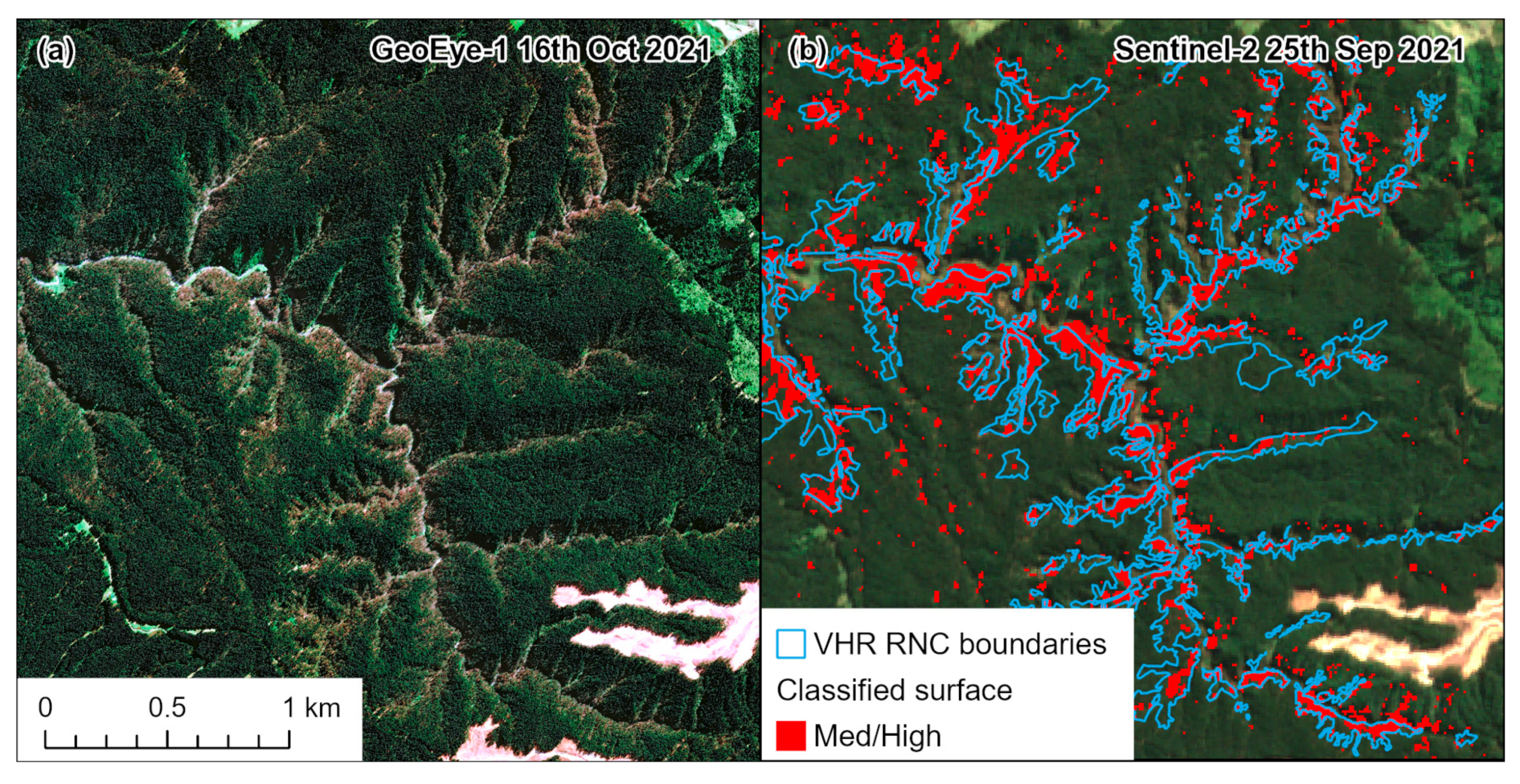
2.1. Spatial Predictions of RNC from Sentinel-2

2.1.1. Study Area and Plantation Delineation

The Gisborne region was selected for this study because of consistent RNC expression in the area, known to be primarily caused by P. pluvialis [2,8,19]. Annual ground visits by experienced forest pathologists between 2019 and 2023 [19] found RNC to be the main forest health issue of radiata pine in this region, with the disease constituting 89% of all 146 inspections (Forest Health Database). Samples of cast needles and accessible symptomatic needles in the lower canopy (Figure 1c) were tested for the presence of Phytophthora pluvialis and P. kernoviae through qPCR [35], and P. pluvialis was detected in the vast majority of cases. In contrast, Dothistroma needle blight symptoms were only observed in ca. 9% of inspections (Forest Health Database) and mainly occurred in very young stands during 2022 and 2023, which is consistent with long term observations showing the severity of Dothistroma needle blight to be relatively low in the Gisborne region [36].

Plantation boundaries within the Gisborne region were mapped using a previously developed deep learning model trained to delineate radiata pine in aerial imagery using a large hand-labeled dataset developed for this task. The model is based on the DeepLabv3+ [37] architecture for semantic segmentation with a ResNet-101-based backbone [38]. The model was used to map the boundaries of pine plantations ranging in scale from shelterbelts and small woodlots through to large forestry estates using 30 cm resolution RGB aerial imagery covering the Gisborne region, which was captured during the summer flying seasons from 2017 to 2019. As an indication of model performance, the Intersection over Union (IoU) on a withheld test set was 0.93. Model predictions were further improved using test-time augmentation to refine the boundary quality. Lastly, a process of semi-automatic cleaning followed by manual inspection of the predictions across the region was carried out. The final forest boundary layer provided a detailed and accurate representation of the spatial extent of all radiata pine plantations across the Gisborne region.

2.1.2. Data Collection

Copernicus Sentinel-2 data were manually reviewed from 2019 to 2023 using Google Earth Engine (GEE) over the Gisborne region of New Zealand, covering UTM grids 60HWB, 60HWC, 60HWD, 60HXC and 60HXD [39]. The Sentinel-2 constellation is a pair of multispectral satellites operated by the European Space Agency (ESA), capturing visible near-infrared (VNIR) and shortwave infrared (SWIR) bands at spatial resolutions ranging from 10 to 60 m [40]. The Bottom-Of-Atmosphere (BOA) Level 2A product was used, which was processed via Sen2Cor from Level 1C Top-Of-Atmosphere (TOA) at ingestion to the GEE image catalogue to produce an analysis-ready dataset [41].

A time series of Sentinel-2 data collected over a known RNC expression site was used to compare changes in four commonly used indices, with respect to the values estimated prior to RNC expression in mid-March 2023. The increases in the Normalized Difference Red/Green Index (NDRG) were markedly greater than the reductions in the other three indices (Figure 2), including the Normalized Difference Vegetation Index (NDVI; NIR and red bands), Enhanced Vegetation Index (EVI; a combination of red, blue and NIR bands), and Normalized Difference Red Edge (NDRE; NIR and Red Edge 1). Substantial increases in NDRG were apparent by June, while consistent reductions in the other three indices did not occur until late July. By the time that maximum RNC expression occurred in mid-September, increases in NDRE from the baseline were 0.425 which markedly exceeded the respective reductions from the baseline of 0.204, 0.203 and 0.159 for NDVI, NDRG and EVI (Figure 2). Based on this comparison, further analyses used NDRG to detect RNC.

For each year, a baseline image capture as close to the beginning of March as cloud cover allowed, was selected (T1). The baseline dates ranged from 11th of February in 2020 to 12th of March in 2022. A visual inspection of the imagery and NDRG time series showed that disease expression tended to peak in September, so corresponding image captures (T2) were selected for each year within this month and included the 13th (2020, 2022, 2023), 25th (2021) and 29th of September (2019).

2.1.3. Satellite Imagery Processing

Images were cloud- and cloud shadow-masked using the Cloud Score+ collection available within GEE and using the cs_cdf band, which describes the likelihood that a given Sentinel-2 pixel is clear on a dimensionless scale of 0 to 1, with 0 representing occlusion and 1 representing a clear observation relative to an estimated distribution of values for that pixel [42]. Given that the target region included a managed plantation forest, harvested areas consisting of large areas of bare earth were present. These areas were masked from analysis by comparing the NDVI values of the T1 and T2 images and eliminating pixels that had a drop of greater than 0.4. A pixel-wise erosion and dilation step was also undertaken within GEE to remove single pixel noise, and a final buffer was applied to avoid the high reflectance from bare soil in the recently clear-felled sites.

The R/G_diff was calculated by subtracting the NDRG of T1 from the NDRG of T2 per pixel for each year, with a scaling factor applied before the export from GEE.

$${\mathrm{R}/\mathrm{G}}_{\mathrm{d}\mathrm{i}\mathrm{f}\mathrm{f}}=\left({\mathrm{N}\mathrm{D}\mathrm{R}\mathrm{G}}_{\mathrm{T}2}-{\mathrm{N}\mathrm{D}\mathrm{R}\mathrm{G}}_{\mathrm{T}1}\right)\times 1000$$

(1)

In addition to the cloud masks, other masks were developed to reduce the incidence of changes not resulting from disease expression, resulting in high R/G_diff values. These included limiting the maximum difference value to 750, as observations showed these generally resulted from canopy loss due to slips or other small total loss events. A simple brightness band was added to both T1 and T2 images by summing the RGB bands, and areas with a brightness too high (generally resulting from cloud or harvest) or too low (from shadow) were masked. Finally, the yearly R/G_diff surfaces were masked to the extent of the forest boundaries to remove any pixels not representative of plantation forest. The resulting masked surfaces were filtered within ArcGIS Pro 3.2.1, using the low pass filter with a 3 × 3 neighborhood.

Figure 3 shows a comparison of Sentinel-2A images acquired (a) before expression (T1) and (b) during peak expression (T2). The filtered R/G_diff surface masked to the forest boundary extent shown in (c) captures the gradient of expression severity visible across the planted area. This image has been subsequently classified into regions (d) without RNC (R/G_diff < 200), and with low (R/G_diff 200–280) and medium–high severity (R/G_diff > 280). The calculation of R/G_diff for two areas with contrasting severity (illustrated in panels c, d) is shown in Figure 3e.

2.1.4. Sampling

A total of 3000 random points per year were generated within the forest boundaries and buffered by 20 m, creating pseudo plots (Figure 4). Plot locations were unique between years, and plots that fell within the areas of noData for each R/G_diff surface (due to masking) were eliminated. This left a total of 12,837 plots, with 2751, 2665, 2640, 2213 and 2568 plots within consecutive years from 2019 to 2023 (Figure 4). The values of R/G_diff were sampled for each year from within the pseudo plots using the Zonal Statistics tool within QGIS 3.28. Figure 3d shows an example of the resulting model data against the classified R/G_diff surface, classed as either expression or no expression depending on the underlying R/G_diff surface values in Figure 3c.

2.2. Weather Data

Weather data that were used in analyses were from the Virtual Climate Station Network (VCSN) supplied by the National Institute of Water and Atmospheric Research (NIWA). The VCSN data provide a national 5 km coverage of a range of weather variables that have been estimated from 150 automatic climate stations owned and operated by NIWA and the MetService. The VCSN data that were used included daily rainfall, maximum (T_max) and minimum air temperature (T_min), relative humidity, solar radiation, and windspeed. As part of the national coverage, estimates of these six variables were available every day over the period of the study (2018–2023) on a 5 km grid throughout the Gisborne region. All six variables were averaged from a daily to a monthly level across the 5 km spatial grid. Inverse distance weighting was then used to create a spatial surface for each climate variable for all months that were used for RNC prediction (i.e., 66 monthly surfaces from October 2018–August 2023), using ArcGIS Pro 3.2.1. September was not included as this was the month that disease expression was determined. Values for each weather variable were then extracted from these surfaces for the locations shown in Figure 4 and aligned with the year in which disease severity was determined (e.g., months from October 2018 to August 2019 were matched with R/G_diff points for September 2019).

2.3. Data Analysis

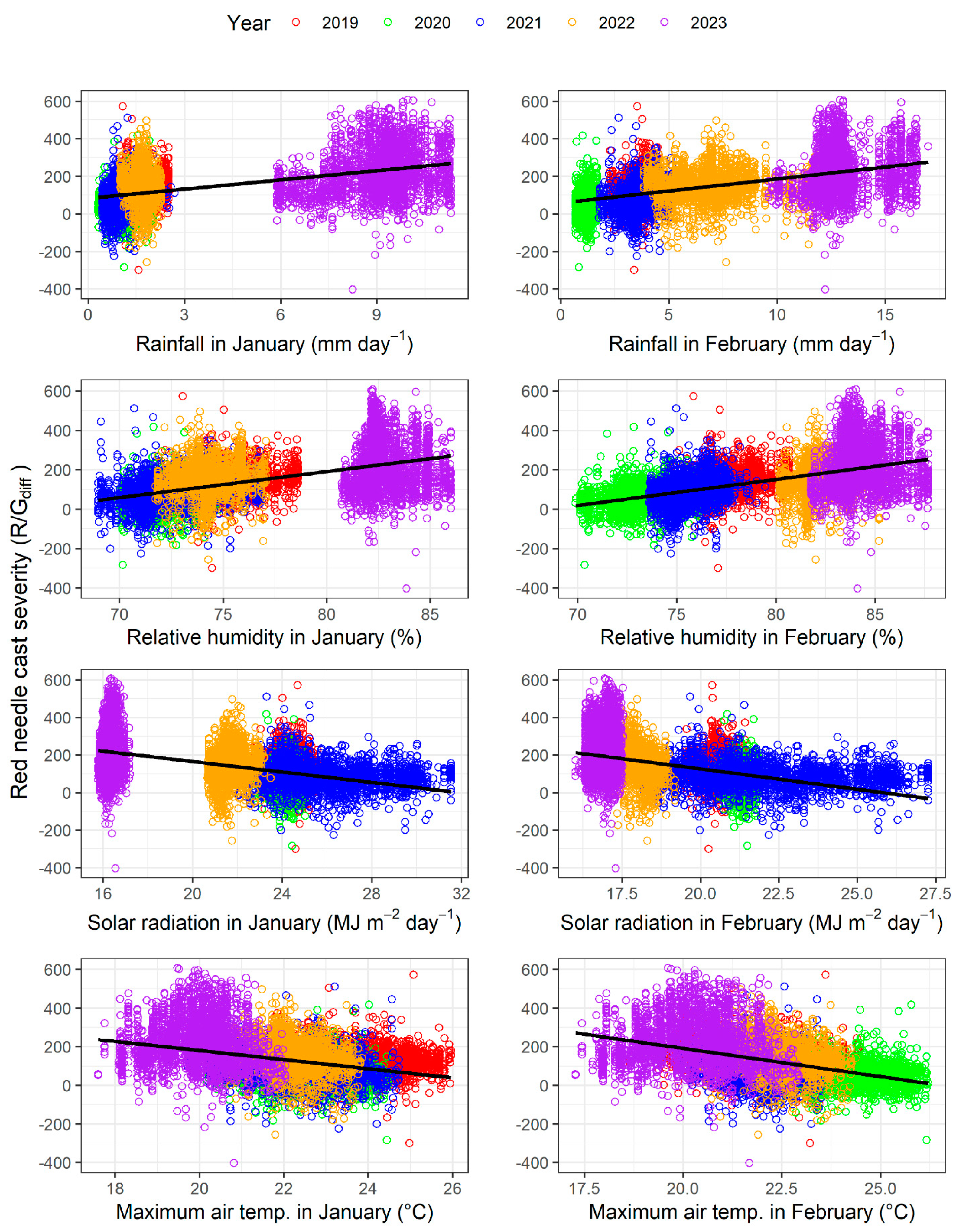
2.3.1. Relationships between R/G_diff and Weather Variables

Using R version 4.2.3. [43], linear models were fitted between R/G_diff and the monthly averages of the six weather variables using the full dataset. In total, this analysis included 66 models, with the predictor variable comprising each of the six weather variables × 11 months. The coefficient of determination (R²) was extracted from all models and plotted against each month to determine the seasonal strength of relationships between the six predictor variables and R/G_diff. The weather variables that were most strongly related to R/G_diff and, for these variables, the months with the strongest correlations were identified. Plots were constructed showing the relationship between R/G_diff and these variable/month combinations.

2.3.2. Classification Model

Random forest was used to classify no expression (No RNC) and the expression of RNC (RNC) from the weather variables using scikit-learn, version 0.23.2 [44] for Python (version 3.8.5). Random forest is an ensemble learning method that creates a collection of decision trees during training. Each tree in the forest is built from a sample drawn with a replacement (bootstrap sample) from the training set, and split decisions are made at each node based on a random subset of these features. This approach enhances diversity among the trees, which reduces overfitting and improves generalization to unseen data. The final classification decision is made based on the majority voting principle, where the class label predicted by the majority of the trees is chosen as the final output, thereby enhancing the accuracy and robustness of the model.

Prior to model development, two data preparation steps were undertaken. To ensure that these two classes were correctly identified within the underlying dataset (n = 12,837), the predictions of R/G_diff were categorized into two groups. Plots with R/G_diff < 200 comprised plots with no RNC (n = 10,533), while values of R/G_diff > 280 comprised plots with RNC (n = 988). Comparisons of these categories with hand-digitized boundaries from VHR GeoEye satellite imagery (pansharpened resolution of 0.5 m) provided accurate RNC delineation across a number of years [19]. The example illustrated in Figure 5 clearly shows that these cutoffs were able to accurately define the two groups through excluding potentially ambiguous observations, without RNC or low severity RNC, with R/G_diff values ranging from 200 to 280. The number of observations within the No RNC group was then randomly sampled so that it matched the number of observations within the RNC group (n = 988 in both groups) to avoid issues with data imbalance between groups [45].

Recursive feature elimination (RFE) was used with the random forest algorithm to subset the predictors to the most important variables. The RFE undertook cross validation and was constrained so that no more than 10 features that had correlations of <0.9 were selected to avoid redundancy and overfitting in the final models. This initial selection was subsequently refined by removing the less important variables during the model fitting process.

Following the feature selection, a stratified split (with respect to the group) was used to divide observations into a training dataset comprising 80% of the observations (n = 1580), with the remaining 20% (n = 396) retained as a test dataset. The random forest model was fitted to the training dataset using a stratified cross validation with predictions from this fitted model made on the independent test dataset. This process was repeated 49 times using a different train/test split during each iteration, and performance statistics were averaged over predictions on all 50 test datasets. This approach removed any potential bias that might have resulted from an unbalanced choice of the test dataset using a single train/test split and providing a more rigorous evaluation of true model performance.

Three hyperparameter grids were evaluated for model fitting that varied in complexity, with the simplest using default parameters and the most complex optimizing model performance across a range of five hyperparameters (the number of estimators, max depth, max features, min samples split, and min samples leaf). The default hyperparameter grid was selected for the final model as this had the best mean performance from the 50 iterations on the test dataset.

Using predictions made on the 50 independent test datasets, a confusion matrix was constructed for each model. As is common practice in experiments where disease is predicted [45], the plots with RNC were designated positive. Using data from the 50 confusion matrices the mean percentage of true positives (TP), true negatives (TN), false positives (FP) and false negatives (FN) was determined.

Model performance was determined from the confusion matrix data using precision, recall, F1 score, and accuracy, which were calculated as follows:

$$\mathrm{P}\mathrm{r}\mathrm{e}\mathrm{c}\mathrm{i}\mathrm{s}\mathrm{i}\mathrm{o}\mathrm{n}=\frac{\mathrm{T}\mathrm{P}}{\mathrm{T}\mathrm{P}+\mathrm{F}\mathrm{P}}$$

(2)

$$\mathrm{R}\mathrm{e}\mathrm{c}\mathrm{a}\mathrm{l}\mathrm{l}=\frac{\mathrm{T}\mathrm{P}}{\mathrm{T}\mathrm{P}+\mathrm{F}\mathrm{N}}$$

(3)

$$\mathrm{F}1\mathrm{s}\mathrm{c}\mathrm{o}\mathrm{r}\mathrm{e}=2\times \frac{\mathrm{P}\mathrm{r}\mathrm{e}\mathrm{c}\mathrm{i}\mathrm{s}\mathrm{i}\mathrm{o}\mathrm{n}\times \mathrm{R}\mathrm{e}\mathrm{c}\mathrm{a}\mathrm{l}\mathrm{l}}{\mathrm{P}\mathrm{r}\mathrm{e}\mathrm{c}\mathrm{i}\mathrm{s}\mathrm{i}\mathrm{o}\mathrm{n}+\mathrm{R}\mathrm{e}\mathrm{c}\mathrm{a}\mathrm{l}\mathrm{l}}$$

(4)

$$\mathrm{A}\mathrm{c}\mathrm{c}\mathrm{u}\mathrm{r}\mathrm{a}\mathrm{c}\mathrm{y}=\frac{\mathrm{T}\mathrm{P}+\mathrm{T}\mathrm{N}}{\mathrm{T}\mathrm{P}+\mathrm{F}\mathrm{P}+\mathrm{T}\mathrm{N}+\mathrm{F}\mathrm{N}}$$

(5)

Precision quantifies the fraction of correct positive predictions, whereas recall identifies the fraction of true positives that were accurately detected. High values of precision mean there are few false positives, while high values of recall indicate low numbers of false negatives. The F1 score represents the harmonic mean of precision and recall, serving as a balanced measure of model discriminatory power. F1 scores span a continuum from 0 to 1, with categorizations from 0.5 to 0.7, 0.7 to 0.8, 0.8 to 0.9, and >0.9, signifying poor, acceptable, excellent, and outstanding levels of discrimination, respectively. Accuracy was defined as the percentage of correctly predicted observations to the total observations.

Using the final fitted model, predictions were made across the Gisborne region. Predictions of disease absence or presence were made for each of the 5 years to visually display the changes between years. These predictions were overlaid with the categorized plots used within the model (RNC, No RNC) to check if model predictions spatially aligned with variations in disease presence/absence identified through R/G_diff.

3. Results

3.1. Variation in RNC Severity

The extracted data showed a wide variation in mean disease severity between the years. R/G_diff varied four-fold across the five years, ranging from 60 in 2020 to 225 in 2023 (

Table 1. Variation in RNC severity (mean ± S.E) and allocation of plots to the four severity classes.

	2019	2020	2021	2022	2023
R/Gdiff	132 (1.1)	60 (1.0)	88 (1.3)	150 (1.7)	225 (2.5)
RNC severity by class (%)
None	89.9	99.0	94.8	77.1	47.3
Low	8.4	0.9	4.3	17.4	21.8
Med	1.6	0.0	0.7	5.0	18.0
High	0.1	0.1	0.2	0.5	12.9

). From the extracted data, plots with disease expression (R/G_diff > 200) ranged from 1% in 2020 to 52.7% in 2023. The percentage of plots with medium/high severity (R/G_diff > 280) was very low during 2020 (only four extracted plots) and relatively low in 2019 and 2021, when these plots comprised 1.7% and 0.9% of the total, respectively. The percentage of plots with medium/high severity increased in 2022, when these plots were 5.5% of the total, and further increased in 2023, when these plots constituted 30.9% of the total (Table 1).

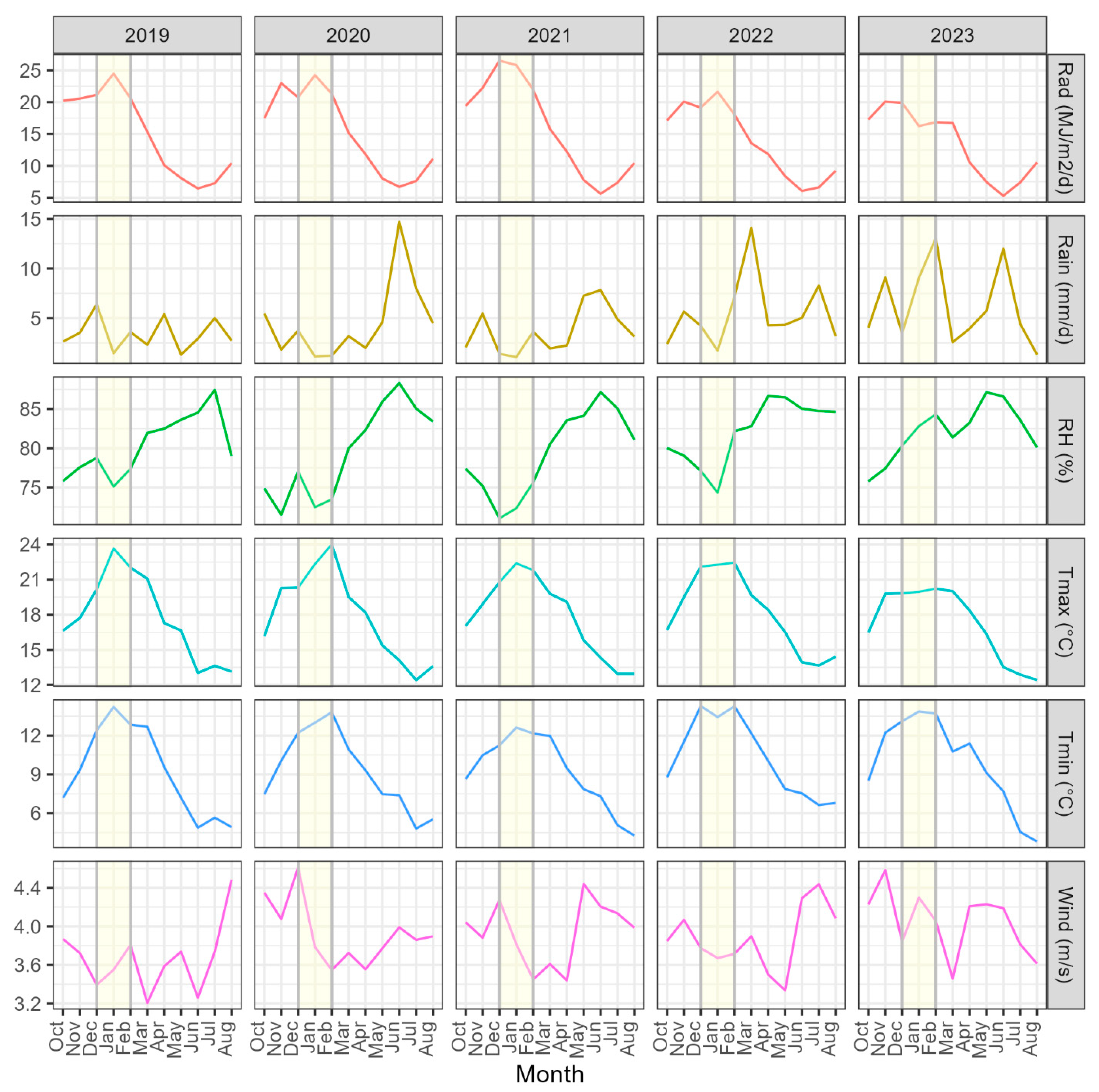
3.2. Variation in Environmental Conditions

Solar radiation in 2019–2021 peaked during summer in December and January at between 24.4 and 26.3 MJ m² day⁻¹ (Figure 6). During 2022 and 2023, summer solar radiation was lower, and values peaked at 21.6 MJ m² day⁻¹ and 19.9 MJ m² day⁻¹, respectively. Rainfall varied widely between months from 2019 to 2021 but, except for June 2020 (14.7 mm day⁻¹), was lower than 8 mm day⁻¹. Although there were marked monthly fluctuations, summer and autumn rainfall during 2022 and 2023 was markedly higher than in the preceding three years, reaching maximum values of 14.1 mm day⁻¹ in March 2022 and 13.1 mm day⁻¹ in February 2023 (Figure 6).

Relative humidity peaked in mid–late winter during all years. However, there was considerable variation in relative humidity between the years during summer. These differences were mostly marked in February, with the values for 2022 and 2023 at 82% and 84% considerably exceeding those of 73–77% between 2019 and 2021 (Figure 6). Although T_max peaked in mid–late summer each year, values were markedly lower in January and February during 2023 (19.9–20.2 °C) compared to those from 2019 to 2022 (21.8–24.0 °C). Changes in T_min over the five-year period followed a similar trend each year, generally peaking in mid-to-late summer, and, with the exceptions of 2020 and 2021, exhibited a similar range between years. There was no clear interannual or seasonal pattern in windspeed (Figure 6).

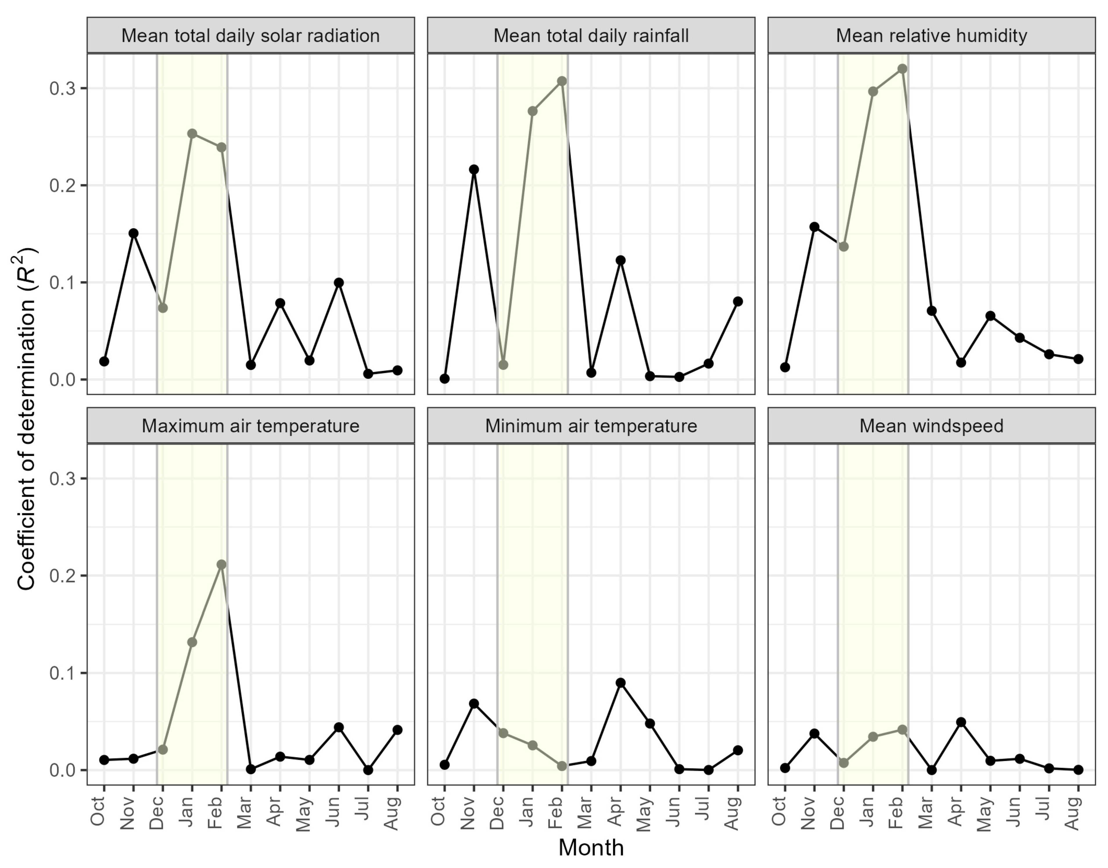
3.3. Relationships with Climatic Variables and Seasonal Patterns

Using the data pooled across all years, the strongest relationships between R/G_diff and weather variables were for relative humidity, rainfall, solar radiation, and T_max (Figure 7). The values for R² generally reached a peak in February and were 0.32, 0.31, 0.24, and 0.21 for relative humidity, rainfall, solar radiation, and T_max, respectively. Relationships between R/G_diff and these four variables during January were of a similar, but generally slightly lower strength. In contrast to these four variables, the strength of relationships between R/G_diff and both T_min and windspeed were relatively weak (Figure 7).

The relationships between the strongest four weather variables and R/G_diff during January and February are shown in Figure 8. Linear lines were fitted to these data, and equation coefficients and the coefficient of determination are given in

Table A1. Model information for linear equations (R/G_diff = a + bx) fitted between RNC severity (R/G_diff) and the four weather variables for January and February shown in Figure 8. Shown are the model coefficients (intercept and slope) and the coefficient of determination (R²) for each equation.

Variable	Month	Intercept	Slope	R2
Rainfall (mm day−1)	January	82.6	16.4	0.28
Relative humidity (%)	January	−866	13.2	0.30
Solar radiation (MJ m−2 day−1)	January	443	−13.9	0.25
Maximum air temperature (°C)	January	653	−23.6	0.13
Rainfall (mm day−1)	February	58.1	12.8	0.31
Relative humidity (%)	February	−910	13.3	0.32
Solar radiation (MJ m−2 day−1)	February	561	−21.7	0.24
Maximum air temperature (°C)	February	777	−29.3	0.21

. During both months, R/G_diff was positively related to rainfall and relative humidity and negatively related to solar radiation and T_max. The ordering of R/G_diff values between the years was relatively consistent with the values for these weather variables. For example, the extracted plots for 2023, which was the year of the worst outbreak, had very high rainfall and relative humidity and very low solar radiation and T_max, with these differences being most marked in January (Figure 8). Similarly, for 2022, which had the second highest values of R/G_diff, the values for these four variables were generally similar but not as extreme as for 2023, particularly for the four February variables. In contrast, the low values of R/G_diff in 2020 were associated with low values of rainfall and relative humidity and high values of solar radiation and T_max, with these patterns being particularly evident during February (Figure 8).

3.4. Classification Model

3.4.1. Variable Selection and Model Performance

The RFE identified eight variables, including relative humidity, T_max, and solar radiation during February, rainfall and T_max during January, November rainfall, March solar radiation, and July relative humidity. This initial model had an accuracy of 89% and F1 score of 0.89. Variables were eliminated from the model without reducing the model performance until the following four variables remained, which are listed in order of importance as follows: mean total daily solar radiation in February, mean relative humidity in February, mean total daily rainfall in January, and mean T_max in February.

The final random forest model with these four variables was able to distinguish the no RNC from RNC plots with a high level of accuracy. Contingency table values for the mean number of TN, FP, FN and TP (with percent in brackets) averaged across all iterations on the test dataset (n = 396) were 175.7 (44%), 22.3 (6%), 22.2 (6%), 175.8 (44%). The accuracy and F1 score were 89% and 0.89, respectively. Recall and precision were both 0.89, indicating that there were a similar number of false positives and incorrect RNC classifications.

3.4.2. Model Predictions

There was excellent agreement between model predictions and the underlying R/G_diff values by year (Figure 9). As with the underlying data, model predictions showed that RNC was most severe in 2023, followed by 2022. An intermediate level of disease occurrence was predicted in 2019 and 2021, and little disease was predicted in 2020.

The predicted location of the disease also shifted substantially between years (Figure 9). In 2022, most diseased areas were predicted to be in the western and southern areas, while in 2023, the disease was mainly concentrated in central and north-eastern parts of the region. Large areas of predicted expression extended beyond the underlying model data showing expression, particularly in the far west during 2022 and around the outskirts of model data during 2023. However, this is in line with expectations as there are very few radiata pine plantations located in these areas (bottom right panel, Figure 9).

4. Discussion

By integrating large scale observations from satellite imagery with climatic data, the developed methodology provides a unique framework for pre-visual disease prediction on a large scale. This method provides an efficient means of identifying the location and severity of the disease well in advance of peak disease expression, which could facilitate more focused monitoring and control programs. From a model development standpoint, the large dataset that can be generated through regional captures of satellite imagery provides a means of more robustly linking diseases, such as RNC, with key determinants of occurrence and severity. Using this method, RNC severity was most strongly correlated with solar radiation, relative humidity, rainfall, and maximum air temperature during mid-to-late summer. The random forest model, which included these four variables, was able to accurately predict the presence of RNC at a large scale.

The methodology developed here provides an effective and low-cost pre-visual prediction method for understanding the location and severity of RNC. As the model utilized summer weather data, predictions of disease incidence for the coming year could be made months in advance of peak disease expression. Regional R/G_diff data acquired during the following spring could then be used to validate predictions and further refine the model. This iterative process provides a framework for continuous predictive improvement through expanding the range and combinations of weather conditions and their impact on disease expression.

The early prediction of RNC has multiple applications. The data layers that have been created can provide baseline regional maps to focus on surveillance and control measures. The real time detection of disease typically relies on aerial sketch-mapping surveillance or spectral data collection from fixed wing aircraft or high-resolution satellites [18,46,47]. As these imagery acquisitions are very expensive, the predictions made here could be used to forecast outbreak years and, within a given year, refine the surveillance radius and eliminate areas unlikely to be at risk.

Predictions could also be used to target preventative sprays to mitigate the impacts of the disease on growth. The sporulation of P. pluvialis typically occurs on asymptomatic tissue, and therefore, preventative control is more likely to be effective than the treatment of visible symptoms identified through monitoring. The application of copper fungicides has been found to protect needles from infection for at least three months [48], and reduce subsequent disease severity [11,49]. The identification of hot spots that are confirmed by ground or aerial surveys from early autumn onwards could provide the basis for the targeted application of copper to reduce infection success, contributing to lower disease severity and impacts on growth later in the year. Areas which are identified as frequent disease hot spots may also inform genotype selections, initially as locations to install breeding trials for RNC resistance and then in the future as areas for the deployment of more resistant radiata pine genotypes or alternative species.

The climatic variables identified as important in this study were consistent with those found in previous research that linked temporal patterns in pathogen sporulation and infection with weather in a limited number of plots and years [8,9]. Our work complements this through the expansion of the study area to a regional scale and examination of symptoms resulting from the cumulative effect of infections over annual epidemics. Our study confirmed the positive relationship between both rainfall and relative humidity and RNC expression, as well as the negative effect of solar radiation and maximum temperature on disease. Recent research [8] monitored the sporulation of P. pluvialis and P. kernoviae over three years at sites in the Gisborne region and central North Island. The detection of inoculum in both species peaked in late winter and was positively linked with rainfall and relative humidity but decreased with increasing temperature, dew point, evaporation, and solar radiation. Windspeed was not significantly related to the presence of either pathogen. Infection has also been monitored on potted plants [9] over a two-year period at sites in the Central North Island. This research found infections to occur predominantly between mid-autumn and early spring during the period of the year when temperatures, solar radiation, and evapotranspiration are at their lowest, relative humidity is at its maximum, and rainfall is plentiful.

Although previous studies have suggested that summer conditions are the limiting phase in the RNC cycle, these data are the first to demonstrate a clear link between weather conditions in summer and the severity of disease during the following autumn, winter, and spring. Previous research has found that inoculum of P. pluvialis and P. kernoviae was not detected for a prolonged period at plots in the Gisborne region and Central North Island after a summer drought during 2012–2013 [8]. This finding was consistent with data from the New Zealand Forest Health Database collected over a 10-year period from 2008 to 2017. Nationally, the lowest numbers of P. pluvialis were reported following the 2012–2013 summer drought. Conversely, the mild and very wet summer during 2011–2012 preceded the highest reported numbers of both pathogens in 2012. The severity of a polycyclic epidemic is determined by the quantity of initial inoculum and the apparent rate of infection as the disease develops [50]. As outlined by [9], we currently have limited knowledge on the persistence mechanisms of these pathogens between epidemics or the impacts of weather variables on this process. It has been suggested that pockets of infection may persist through summer, which may present the source of outbreaks in the following autumn [9]. The opposite trend has also been hypothesized, in which trees that have suffered severe defoliation in the previous year may have a reduced severity due to the reduced availability of host tissue [4] and less favorable microclimate in lower density crowns [8].

Our current study supports the hypothesis that weather conditions impacting the levels of initial inoculum (i.e., summer conditions) are important for determining disease severity later in the epidemic and, thus, drive between-year variation in disease expression. We predict that during mild and wet summers, the infection cycle continues, whereas in warmer and drier summers, the infection cycle is unable to continue except in pockets with suitable microclimate. Summer weather, therefore, determines the base level of pathogen presence and abundance the following autumn and, under conditions that are generally favorable for infection rates, supports an exponential increase in resulting symptoms. There is still a need to understand the persistence mechanism of P. pluvialis to understand the impact of disease history on future expression. Although this work has clearly demonstrated the importance of summer weather, in particular late summer conditions, it is important to note the occurrence of a prolonged La Niña system between late 2020 and early 2023, with extreme rain events in later summer 2022 and 2023. Consecutive wet summers during this period may have had an additive effect on the resulting exceptional disease outbreak in 2023. Continued data capture and re-analysis could further our understanding of these processes.

The system developed here integrates multiple foundational elements that enhance the practical deployment and scalability of the methodology. The forest boundaries developed using deep learning provide an accurate base layer that defines the plantation extent. This layer, developed from aerial RGB imagery, helps constrain the monitoring area to plantation boundaries, thereby reducing the volume of Sentinel 2 data that needs to be analyzed to run the detection process. The simplicity of the R/G index allows the RNC detection approach to be generalized to other platforms, as many unmanned aerial vehicles (UAVs) or fixed-wing platforms use camera systems that still capture RGB or true color images. The R/G index is quick to implement and requires less computation than a traditional image classification approach that requires the manual identification of training sites. Further, classification approaches require constant review to ensure training sites are transferable between image captures. This is a slow and computationally expensive activity requiring whole image analysis.

Further research should use outputs from this approach to improve our understanding of RNC. When combined with past predictions from time series satellite coverage, model predictions using weather data provide a comprehensive understanding of areas likely to be affected by disease over both the short and long term. The predictive maps created could be used to place field plots spanning a severity range for determining the impact of spray on disease and the effects of RNC on growth.

As this framework was based on national climate datasets, the system could be readily deployed to other regions. Ideally, predictions outside of the Gisborne region should be based on a model that is built from the weather of the new region. Although model predictions in random forests can be made outside of the fitted data range, these empirical predictions are likely to be more robust when the fitted data range covers the range and combination of input variables used for predictions [51,52,53].

The modeling framework developed here has global applicability and could be useful for detecting outbreaks of other pests or diseases on a range of species. All the underpinning datasets that were used are widely available and are usually low-cost or free. Sentinel-2 has global coverage [54], while many countries have regional RGB imagery collected at a very high resolution [55] and weather data that can describe past conditions for a range of important variables [30,31,56]. This method is likely to be most useful for pests and diseases with clearly discernible symptoms visible from satellite data that are expressed within the upper canopy.

5. Conclusions

A novel methodology that integrated Sentinel-2 satellite observations and weather data was used to pre-visually predict the location of RNC over five consecutive years (2019–2023) within radiata pine forests in the Gisborne region. Sentinel-2 imagery was used to characterize the severity of RNC within the region using the difference in the R/G index between the time of maximum expression and no expression of RNC (R/G_diff). Values of R/G_diff were most strongly related to solar radiation, rainfall, relative humidity, and maximum air temperature during mid–late summer, which was 7–8 months prior to the peak expression in the following spring. Using a balanced dataset of 1976 plots, which were disease-free or showed expression of RNC, a random forest model was constructed from these four variables to pre-visually predict the incidence of RNC. Using a hold-out test dataset, the model had excellent performance with an accuracy of 89% and an F1 score of 0.89. The pre-visual prediction of RNC using this model could be used to focus monitoring and treatment to reduce the impact of this disease during the following spring.

References

1. NZFOA. New Zealand Forestry Industry, Facts and Figures 2022/2023. New Zealand Plantation Forest Industry. New Zealand Forest Owners Association, Wellington, 2023. Available online: https://www.nzfoa.org.nz/images/Facts_and_Figures_2022-2023_-_WEB.pdf (accessed on 11 March 2024).
2. Dick, M.A.; Williams, N.M.; Bader, M.K.-F.; Gardner, J.F.; Bulman, L.S. Pathogenicity of Phytophthora pluvialis to Pinus radiata and its relation with red needle cast disease in New Zealand. New Zealand J. For. Sci. 2014, 44, 6. [Google Scholar] [CrossRef]
3. Graham, N.J.; Suontama, M.; Pleasants, T.; Li, Y.; Bader, M.K.F.; Klápště, J.; Dungey, H.S.; Williams, N.M. Assessing the genetic variation of tolerance to red needle cast in a Pinus radiata breeding population. Tree Genet. Genom. 2018, 14, 55. [Google Scholar] [CrossRef]
4. Gomez-Gallego, M.; Gommers, R.; Bader, M.K.-F.; Williams, N.M. Modelling the key drivers of an aerial Phytophthora foliar disease epidemic, from the needles to the whole plant. PLoS ONE 2019, 14, e0216161. [Google Scholar] [CrossRef] [PubMed]
5. Ganley, R.J.; Williams, N.M.; Rolando, C.A.; Hood, I.A.; Dungey, H.S.; Beets, P.N.; Bulman, L.S. Management of red needle cast caused by Phytophthora pluvialis a new disease of radiata pine in New Zealand. New Zealand Plant Prot. 2014, 67, 48–53. [Google Scholar] [CrossRef]
6. Reeser, P.; Sutton, W.; Hansen, E.M. Phytophthora pluvialis, a new species from mixed tanoak-Douglas-fir forests of western Oregon, USA. North Am. Fungi 2013, 8, 1–8. [Google Scholar] [CrossRef]
7. Shelley, B.A.; Luster, D.G.; Garrett, W.M.; McMahon, M.B.; Widmer, T.L. Effects of temperature on germination of sporangia, infection and protein secretion by Phytophthora kernoviae. Plant Pathol. 2018, 67, 719–728. [Google Scholar] [CrossRef]
8. Fraser, S.; Gomez-Gallego, M.; Gardner, J.; Bulman, L.S.; Denman, S.; Williams, N.M. Impact of weather variables and season on sporulation of Phytophthora pluvialis and Phytophthora kernoviae. For. Pathol. 2020, 50, e12588. [Google Scholar] [CrossRef]
9. Hood, I.A.; Husheer, S.; Gardner, J.F.; Evanson, T.W.; Tieman, G.; Banham, C.; Wright, L.A.H.; Fraser, S. Infection periods of Phytophthora pluvialis and Phytophthora kernoviae in relation to weather variables and season in Pinus radiata forests in New Zealand. New Zealand J. For. Sci. 2022, 52, 17. [Google Scholar] [CrossRef]
10. Bulman, L.S.; Bradshaw, R.E.; Fraser, S.; Martín-García, J.; Barnes, I.; Musolin, D.L.; La Porta, N.; Woods, A.J.; Diez, J.J.; Koltay, A.; et al. A worldwide perspective on the management and control of Dothistroma needle blight. For. Pathol. 2016, 46, 472–488. [Google Scholar] [CrossRef]
11. Fraser, S.; Baker, M.; Pearse, G.; Todoroki, C.L.; Estarija, H.J.; Hood, I.A.; Bulman, L.S.; Somchit, C.; Rolando, C.A. Efficacy and optimal timing of low-volume aerial applications of copper fungicides for the control of red needle cast of pine. New Zealand J. For. Sci. 2022, 52, 18. [Google Scholar] [CrossRef]
12. Bárta, V.; Lukeš, P.; Homolová, L. Early detection of bark beetle infestation in Norway spruce forests of Central Europe using Sentinel-2. Int. J. Appl. Earth Obs. Geoinf. 2021, 100, 102335. [Google Scholar] [CrossRef]
13. Bozzini, A.; Francini, S.; Chirici, G.; Battisti, A.; Faccoli, M. Spruce bark beetle outbreak prediction through automatic classification of Sentinel-2 imagery. Forests 2023, 14, 1116. [Google Scholar] [CrossRef]
14. Dalponte, M.; Cetto, R.; Marinelli, D.; Andreatta, D.; Salvadori, C.; Pirotti, F.; Frizzera, L.; Gianelle, D. Spectral separability of bark beetle infestation stages: A single-tree time-series analysis using Planet imagery. Ecol. Indic. 2023, 153, 110349. [Google Scholar] [CrossRef]
15. Senf, C.; Pflugmacher, D.; Wulder, M.A.; Hostert, P. Characterizing spectral–temporal patterns of defoliator and bark beetle disturbances using Landsat time series. Remote Sens. Environ. 2015, 170, 166–177. [Google Scholar] [CrossRef]
16. Panzavolta, T.; Bracalini, M.; Benigno, A.; Moricca, S. Alien invasive pathogens and pests harming trees, forests, and plantations: Pathways, global consequences and management. Forests 2021, 12, 1364. [Google Scholar] [CrossRef]
17. Wingfield, M.J.; Slippers, B.; Wingfield, B.D. Novel Associations between Pathogens, Insects and Tree Species Threaten World Forests; University of Pretoria: Pretoria, South Africa, 2010. [Google Scholar]
18. Poona, N.K.; Ismail, R. Discriminating the occurrence of pitch canker fungus in Pinus radiata trees using QuickBird imagery and artificial neural networks. South. For. J. For. Sci. 2013, 75, 29–40. [Google Scholar] [CrossRef]
19. Camarretta, N.; Pearse, G.D.; Steer, B.S.C.; McLay, E.; Fraser, S.; Watt, M.S. Automatic Detection of Phytophthora pluvialis Outbreaks in Radiata Pine Plantations Using Multi-Scene, Multi-Temporal Satellite Imagery. Remote Sens. 2024, 16, 338. [Google Scholar] [CrossRef]
20. Mantas, V.; Fonseca, L.; Baltazar, E.; Canhoto, J.; Abrantes, I. Detection of tree decline (Pinus pinaster Aiton) in European forests using Sentinel-2 data. Remote Sens. 2022, 14, 2028. [Google Scholar] [CrossRef]
21. Migas-Mazur, R.; Kycko, M.; Zwijacz-Kozica, T.; Zagajewski, B. Assessment of Sentinel-2 images, support vector machines and change detection algorithms for bark beetle outbreaks mapping in the Tatra mountains. Remote Sens. 2021, 13, 3314. [Google Scholar] [CrossRef]
22. Venter, Z.S.; Barton, D.N.; Chakraborty, T.; Simensen, T.; Singh, G. Global 10 m land use land cover datasets: A comparison of dynamic world, world cover and esri land cover. Remote Sens. 2022, 14, 4101. [Google Scholar] [CrossRef]
23. Hernández-Clemente, R.; Hornero, A.; Mottus, M.; Penuelas, J.; González-Dugo, V.; Jiménez, J.C.; Suárez, L.; Alonso, L.; Zarco-Tejada, P.J. Early Diagnosis of Vegetation Health From High-Resolution Hyperspectral and Thermal Imagery: Lessons Learned from Empirical Relationships and Radiative Transfer Modelling. Curr. For. Rep. 2019, 5, 169–183. [Google Scholar] [CrossRef]
24. Hornero, A.; Zarco-Tejada, P.J.; Quero, J.L.; North, P.R.J.; Ruiz-Gómez, F.J.; Sánchez-Cuesta, R.; Hernandez-Clemente, R. Modelling hyperspectral-and thermal-based plant traits for the early detection of Phytophthora-induced symptoms in oak decline. Remote Sens. Environ. 2021, 263, 112570. [Google Scholar] [CrossRef]
25. Mahlein, A.K.; Rumpf, T.; Welke, P.; Dehne, H.W.; Plümer, L.; Steiner, U.; Oerke, E.C. Development of spectral indices for detecting and identifying plant diseases. Remote Sens. Environ. 2013, 128, 21–30. [Google Scholar] [CrossRef]
26. Poblete, T.; Camino, C.; Beck, P.S.A.; Hornero, A.; Kattenborn, T.; Saponari, M.; Boscia, D.; Navas-Cortes, J.A.; Zarco-Tejada, P.J. Detection of Xylella fastidiosa infection symptoms with airborne multispectral and thermal imagery: Assessing bandset reduction performance from hyperspectral analysis. ISPRS J. Photogramm. Remote Sens. 2020, 162, 27–40. [Google Scholar] [CrossRef]
27. Tian, L.; Xue, B.; Wang, Z.; Li, D.; Yao, X.; Cao, Q.; Zhu, Y.; Cao, W.; Cheng, T. Spectroscopic detection of rice leaf blast infection from asymptomatic to mild stages with integrated machine learning and feature selection. Remote Sens. Environ. 2021, 257, 112350. [Google Scholar] [CrossRef]
28. Zarco-Tejada, P.J.; Camino, C.; Beck, P.S.A.; Calderon, R.; Hornero, A.; Hernández-Clemente, R.; Kattenborn, T.; Montes-Borrego, M.; Susca, L.; Morelli, M.; et al. Previsual symptoms of Xylella fastidiosa infection revealed in spectral plant-trait alterations. Nat. Plants 2018, 4, 432–439. [Google Scholar] [CrossRef] [PubMed]
29. Calderón, R.; Navas-Cortés, J.A.; Zarco-Tejada, P.J. Early detection and quantification of Verticillium wilt in olive using hyperspectral and thermal imagery over large areas. Remote Sens. 2015, 7, 5584–5610. [Google Scholar] [CrossRef]
30. Lee, E.H.; Beedlow, P.A.; Waschmann, R.S.; Burdick, C.A.; Shaw, D.C. Tree-ring analysis of the fungal disease Swiss needle cast in western Oregon coastal forests. Can. J. For. Res. 2013, 43, 677–690. [Google Scholar] [CrossRef]
31. Lech, P.; Mychayliv, O.; Hildebrand, R.; Orman, O. Weather Conditions Drive the Damage Area Caused by Armillaria Root Disease in Coniferous Forests across Poland. Plant Pathol. J. 2023, 39, 548–565. [Google Scholar] [CrossRef]
32. Ades, P.K.; Simpson, J.A.; Eldridge, K.G.; Eldridge, R.H. Genetic variation in susceptibility to Dothistroma needle blight among provenances and families of Pinus muricata. Can. J. For. Res. 1992, 22, 1111–1117. [Google Scholar] [CrossRef]
33. Woods, A.; Coates, K.; Hamann, A. Is an unprecedented Dothistroma needle blight epidemic related to climate change? BioScience 2005, 55, 761–769. [Google Scholar] [CrossRef]
34. Bulman, L.S.; Dick, M.A.; Ganley, R.J.; McDougal, R.L.; Schwelm, A.; Bradshaw, R.E.; Gonthier, P.; Nicolotti, G. Dothistroma needle blight. In Infectious Forest Diseases; Gonthier, P., Nicolotti, G., Eds.; CPI Group (UK) Ltd.: Croydon, UK, 2013; pp. 436–457. [Google Scholar]
35. McDougal, R.L.; Cunningham, L.; Hunter, S.; Caird, A.; Flint, H.; Lewis, A.; Ganley, R.J. Molecular detection of Phytophthora pluvialis, the causal agent of red needle cast in Pinus radiata. J. Microbiol. Methods 2021, 189, 106299. [Google Scholar] [CrossRef] [PubMed]
36. Watt, M.S.; Tan, A.Y.S.; Fraser, S.; Bulman, L.S. Use of advanced modelling methods to predict dothistroma needle blight on Pinus radiata at a fine resolution within New Zealand. For. Ecol. Manage. 2021, 492, 119226. [Google Scholar] [CrossRef]
37. Chen, L.-C.; Zhu, Y.; Papandreou, G.; Schroff, F.; Adam, H. Encoder-decoder with atrous separable convolution for semantic image segmentation. In Proceedings of the European Conference on Computer Vision (ECCV), Online, 6 October 2018; pp. 801–818. [Google Scholar]
38. He, K.; Zhang, X.; Ren, S.; Sun, J. Deep residual learning for image recognition. In Proceedings of the IEEE Conference on Computer Vision and Pattern Recognition, Vegas, NV, USA, 27–30 June 2016; pp. 770–778. [Google Scholar]
39. Gorelick, N.; Hancher, M.; Dixon, M.; Ilyushchenko, S.; Thau, D.; Moore, R. Google Earth Engine: Planetary-scale geospatial analysis for everyone. Remote Sens. Environ. 2017, 202, 18–27. [Google Scholar] [CrossRef]
40. Drusch, M.; Del Bello, U.; Carlier, S.; Colin, O.; Fernandez, V.; Gascon, F.; Hoersch, B.; Isola, C.; Laberinti, P.; Martimort, P. Sentinel-2: ESA’s optical high-resolution mission for GMES operational services. Remote Sens. Environ. 2012, 120, 25–36. [Google Scholar] [CrossRef]
41. Main-Knorn, M.; Pflug, B.; Louis, J.; Debaecker, V.; Müller-Wilm, U.; Gascon, F. Sen2Cor for sentinel-2. In Proceedings of the Image and Signal Processing for Remote Sensing XXIII, SPIE, Warsaw, Poland, 4 October 2017; Volume 10427, pp. 37–48. [Google Scholar]
42. Pasquarella, V.J.; Brown, C.F.; Czerwinski, W.; Rucklidge, W.J. Comprehensive Quality Assessment of Optical Satellite Imagery Using Weakly Supervised Video Learning. In Proceedings of the IEEE/CVF Conference on Computer Vision and Pattern Recognition, Vancouver, BC, Canada, 17–24 June 2023; pp. 2124–2134. [Google Scholar]
43. R Core Team. R: A Language and Environment for Statistical Computing; R Foundation for Statistical Computing: Vienna, Austria, 2023; Available online: https://www.R-project.org/ (accessed on 15 January 2024).
44. Pedregosa, F.; Varoquaux, G.; Gramfort, A.; Michel, V.; Thirion, B.; Grisel, O.; Blondel, M.; Prettenhofer, P.; Weiss, R.; Dubourg, V. Scikit-learn: Machine Learning in Python. J. Mach. Learn.Res. 2011, 12, 2825–2830. [Google Scholar]
45. Yuan, X.; Chen, S.; Sun, C.; Yuwen, L. A novel early diagnostic framework for chronic diseases with class imbalance. Sci. Rep. 2022, 12, 8614. [Google Scholar] [CrossRef] [PubMed]
46. Coops, N.; Stanford, M.; Old, K.; Dudzinski, M.; Culvenor, D.; Stone, C. Assessment of dothistroma needle blight of Pinus radiata using airborne hyperspectral imagery. Phytopathology 2003, 93, 1524–1532. [Google Scholar] [CrossRef] [PubMed]
47. Leckie, D.; Jay, C.; Gougeon, F.; Sturrock, R.; Paradine, D. Detection and assessment of trees with Phellinus weirii (laminated root rot) using high resolution multi-spectral imagery. Int. J. Remote Sens. 2004, 25, 793–818. [Google Scholar] [CrossRef]
48. Rolando, C.A.; Dick, M.A.; Gardner, J.; Bader, M.K.F.; Williams, N.M. Chemical control of two Phytophthora species infecting the canopy of Monterey pine (Pinus radiata). For. Pathol. 2017, 47, e12327. [Google Scholar] [CrossRef]
49. Rolando, C.; Somchit, C.; Bader, M.K.F.; Fraser, S.; Williams, N. Can copper be used to treat foliar Phytophthora infections in Pinus radiata? Plant Dis. 2019, 103, 1828–1834. [Google Scholar] [CrossRef] [PubMed]
50. Van der Plank, J.E. Plant Diseases: Epidemics and Control; Academic Press: New York, NY, USA, 1963; p. 349. [Google Scholar]
51. Sabatia, C.O.; Burkhart, H.E. Predicting site index of plantation loblolly pine from biophysical variables. For. Ecol. Manag. 2014, 326, 142–156. [Google Scholar] [CrossRef]
52. González-Rodríguez, M.Á.; Diéguez-Aranda, U. Rule-based vs parametric approaches for developing climate-sensitive site index models: A case study for Scots pine stands in northwestern Spain. Ann. For. Sci. 2021, 78, 23. [Google Scholar] [CrossRef]
53. Watt, M.; Moore, J.R. Modelling spatial variation in radiata pine slenderness (height/diameter ratio) and vulnerability to wind damage under current and future climate in New Zealand. Front. For. Glob. Chang. 2023, 6, 1188094. [Google Scholar] [CrossRef]
54. Spoto, F.; Sy, O.; Laberinti, P.; Martimort, P.; Fernandez, V.; Colin, O.; Hoersch, B.; Meygret, A. Overview of Sentinel-2. In Proceedings of the 2012 IEEE International Geoscience and Remote Sensing Symposium, Munich, Germany, 22–27 July 2012; pp. 1707–1710. [Google Scholar]
55. Schepaschenko, D.; See, L.; Lesiv, M.; Bastin, J.-F.; Mollicone, D.; Tsendbazar, N.-E.; Bastin, L.; McCallum, I.; Laso Bayas, J.C.; Baklanov, A. Recent advances in forest observation with visual interpretation of very high-resolution imagery. Surv. Geophys. 2019, 40, 839–862. [Google Scholar] [CrossRef]
56. Gavilán-Acuña, G.; Olmedo, G.F.; Mena-Quijada, P.; Guevara, M.; Barría-Knopf, B.; Watt, M.S. Reducing the Uncertainty of Radiata Pine Site Index Maps Using an Spatial Ensemble of Machine Learning Models. Forests 2021, 12, 77. [Google Scholar] [CrossRef]
Figure 1. Overview of RNC disease symptoms showing (a) full expression at the stand level, (b) intermediate expression, showing how discoloration moves from the lower canopy upwards and (c) a close up of the needles affected by RNC. Photo credits (a) Bryan McKinlay; (b,c) Emily McLay.
Remotesensing 16 01401 g001
Figure 2. Changes in differences of four vegetation indices from a baseline during March 2023 (T1) for an area that showed RNC expression in September 2023. The four indices used to determine these differences were extracted using Sentinel-2 2A time-series data, and included the Enhanced Vegetation index (EVI), Normalized Difference Red Edge (NDRE), Normalized Difference Red/Green Index (NDRG) and Normalized Difference Vegetation Index (NDVI). The vertical lines Time 1 (T1) and Time 2 (T2) represent acquisition dates that included, respectively, a baseline (no expression) and the time of maximum RNC expression.
Remotesensing 16 01401 g002
Figure 3. Sentinel-2 images acquired on (a) 9 March (T1) and (b) 13 September 2023 (T2). Also shown is (c) R/Gdiff determined from these images and (d) R/Gdiff values classified into three classes. For selected areas with no expression and RNC expression (shown in (c,d)), the R/Gdiff calculation is displayed in panel (e) with R/Gdiff for both classes determined as the difference in R/G between Time 2 (T2) and Time 1 (T1).
Remotesensing 16 01401 g003
Figure 4. Distribution of R/Gdiff plots (red points) extracted from within the radiata pine forested areas (grey area) of the Gisborne region.
Remotesensing 16 01401 g004
Figure 5. Comparison of a (a) Maxar GeoEye-1 very high resolution (VHR) 0.5 m pansharpened image captured in October 2021 with the (b) T2 Sentinel-2 image captured in September 2021. Hand-digitalized boundaries of RNC derived from the GeoEye-1 image in (a) are shown in (b), and also overlaid are R/Gdiff values > 280 (Med/High classes) for 2021 derived from the T2 Sentinel-2 image.
Remotesensing 16 01401 g005
Figure 6. Variation in key climatic variables by year and month, that included from top to bottom mean total daily solar radiation, mean total daily rainfall, mean relative humidity, mean maximum (Tmax) and minimum (Tmin) air temperature, and mean windspeed. The displayed months are in chronological order from October to August inclusive, with this period ending immediately before maximum disease expression (September) in the displayed year (i.e., 2019–2023). September is not displayed as final estimates of RNC severity were taken mid-way through the month, and data from this month were not used for model development. The summer months are shaded yellow to provide a point of reference on the figure.
Remotesensing 16 01401 g006
Figure 7. Variation in the coefficient of determination (R2) for linear relationships between each of the displayed weather variables and RNC severity (R/Gdiff), by month, using pooled data from all years. The summer months are shaded yellow to provide a point of reference on the figure.
Remotesensing 16 01401 g007
Figure 8. Relationship between RNC severity (R/Gdiff) and from top to bottom, mean total daily rainfall, mean relative humidity, mean total daily solar radiation and maximum air temperature during (left panels) January and (right panels) February by year.
Remotesensing 16 01401 g008
Figure 9. Predictions from the model showing no expression (grey shade) and expression of RNC (orange shade) by year. Overlaid on these predictions are the model data, derived from Sentinel R/Gdiff, showing no expression (white circles) and expression (red circles). Also shown (bottom right panel) are the radiata pine forested areas within the Gisborne region.
Remotesensing 16 01401 g009