
Mapping Annual Tidal Flat Loss and Gain in the Micro-Tidal Area Integrating Dual Full-Time Series Spectral Indices

 ,
,  ,
,  ,
,
Abstract
1. Introduction
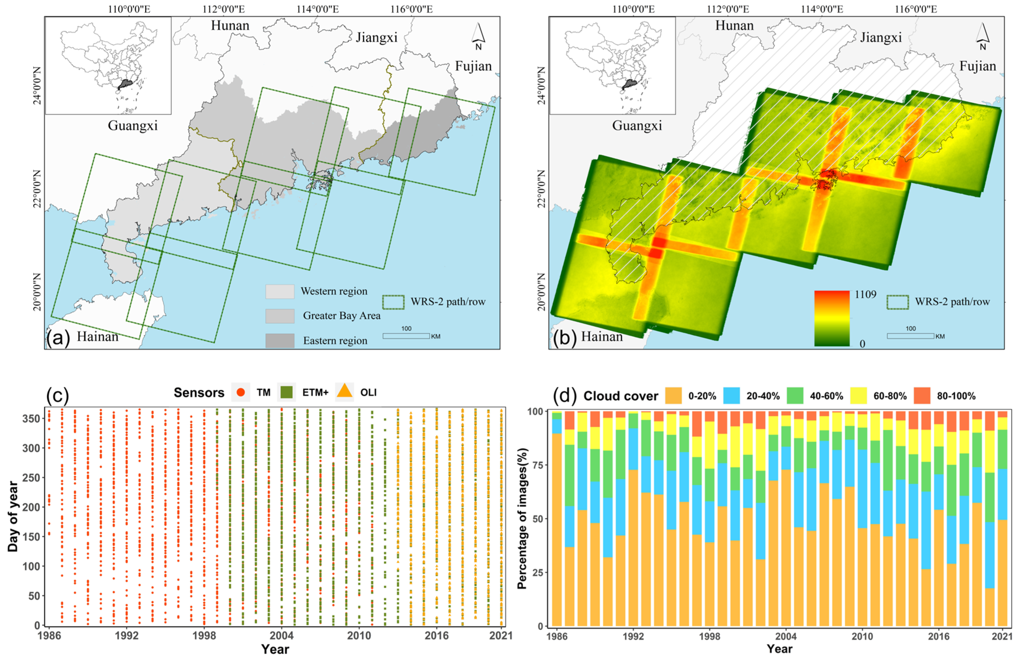
2. The Study Area and the Dataset
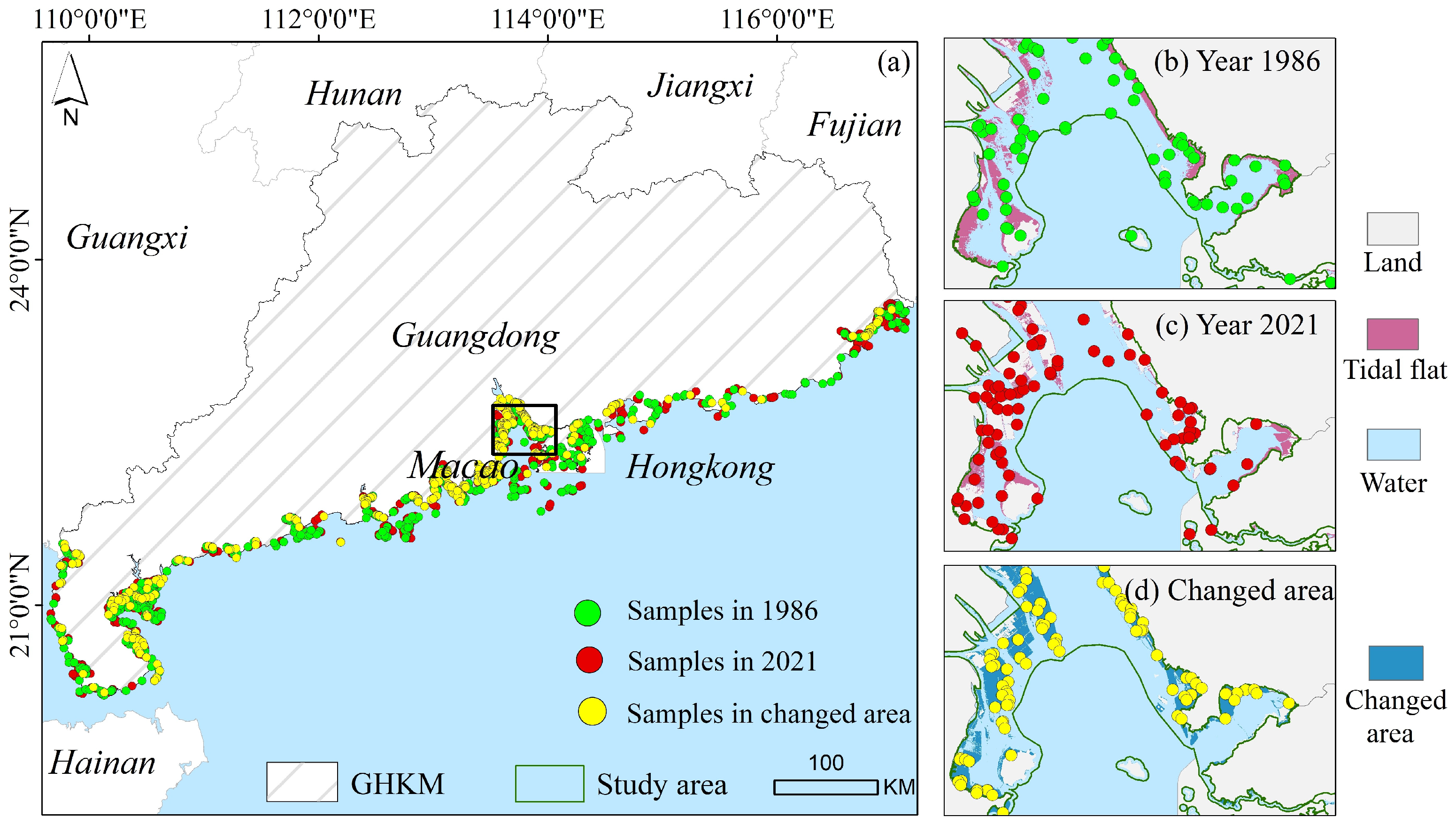
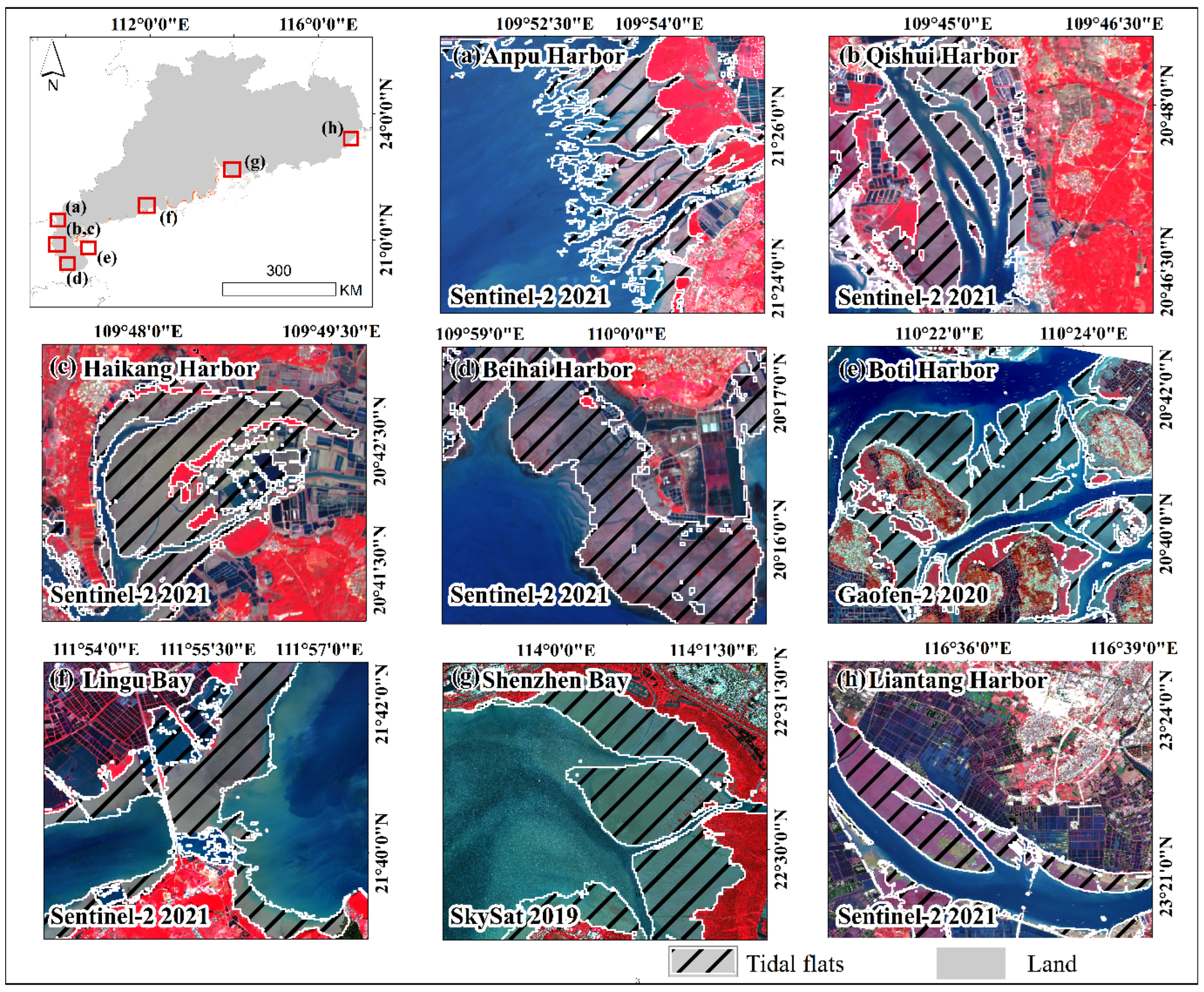
2.1. The Study Area
2.2. The Dataset
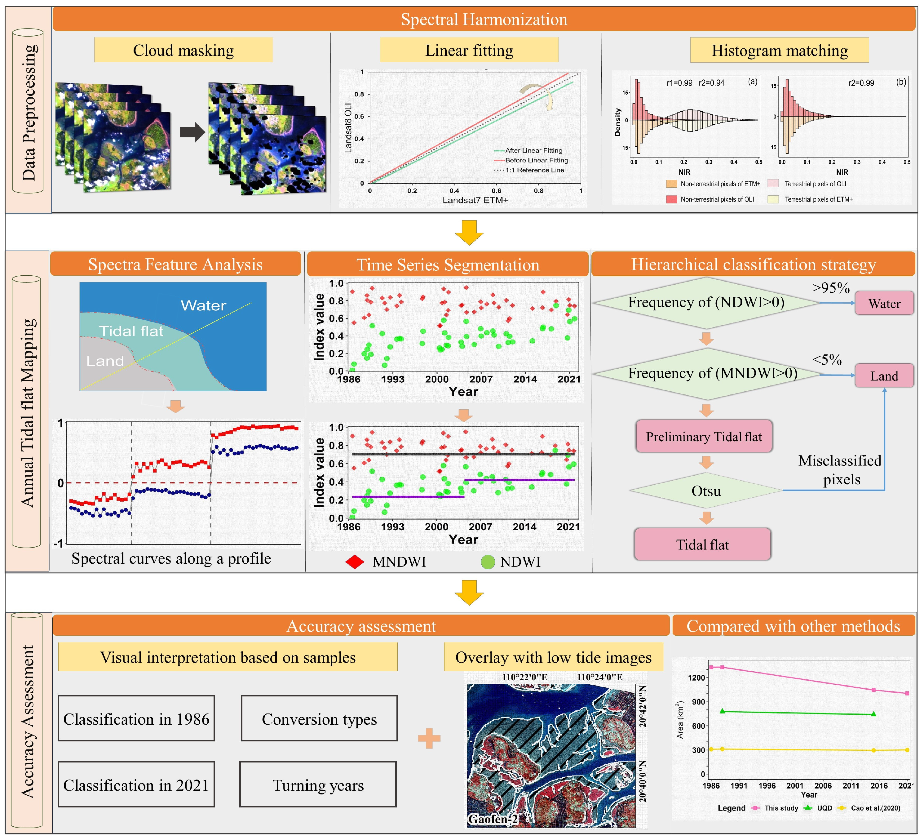
3. Methodology
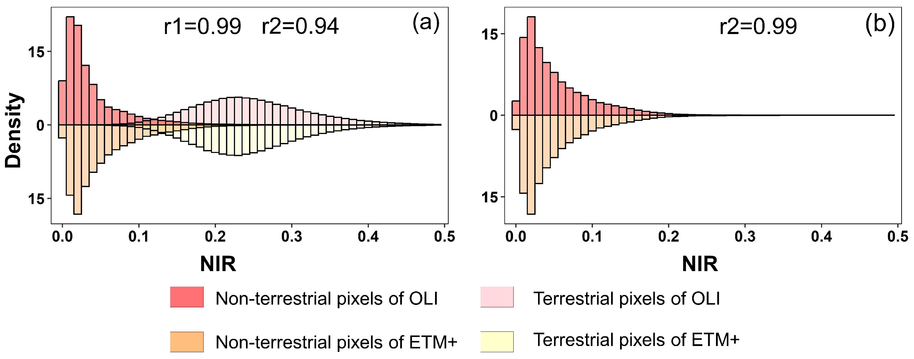
3.1. Spectral Harmonization
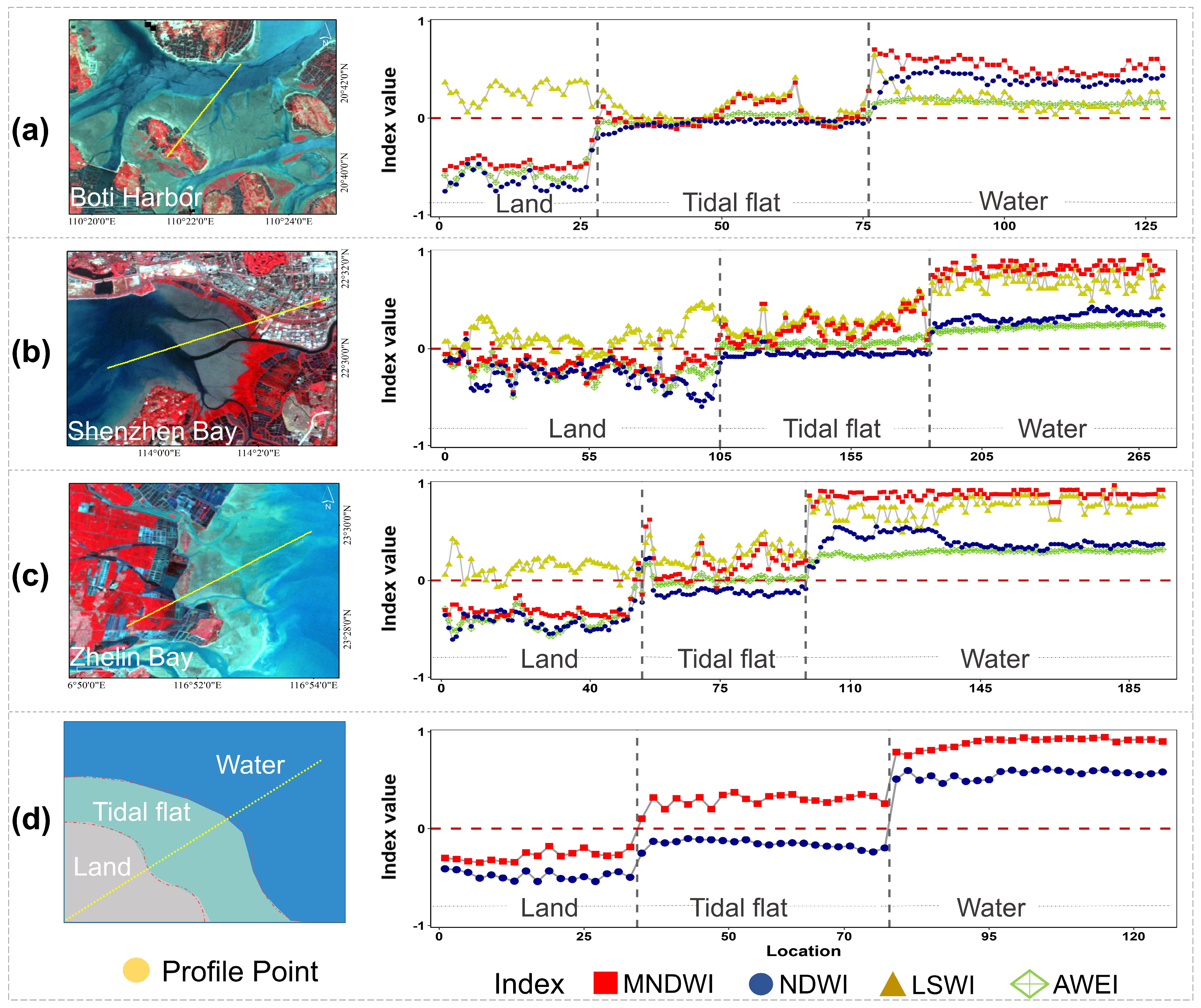
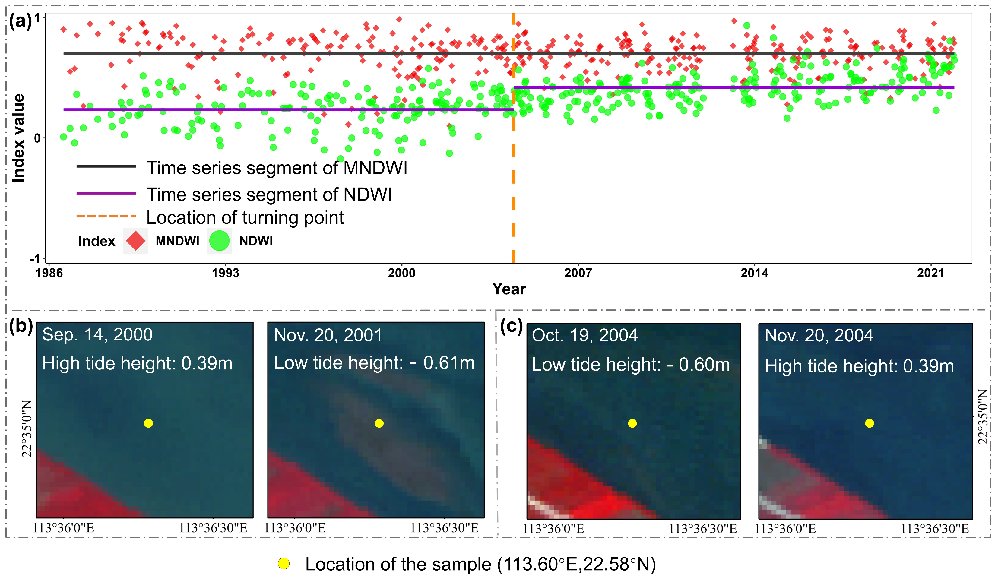
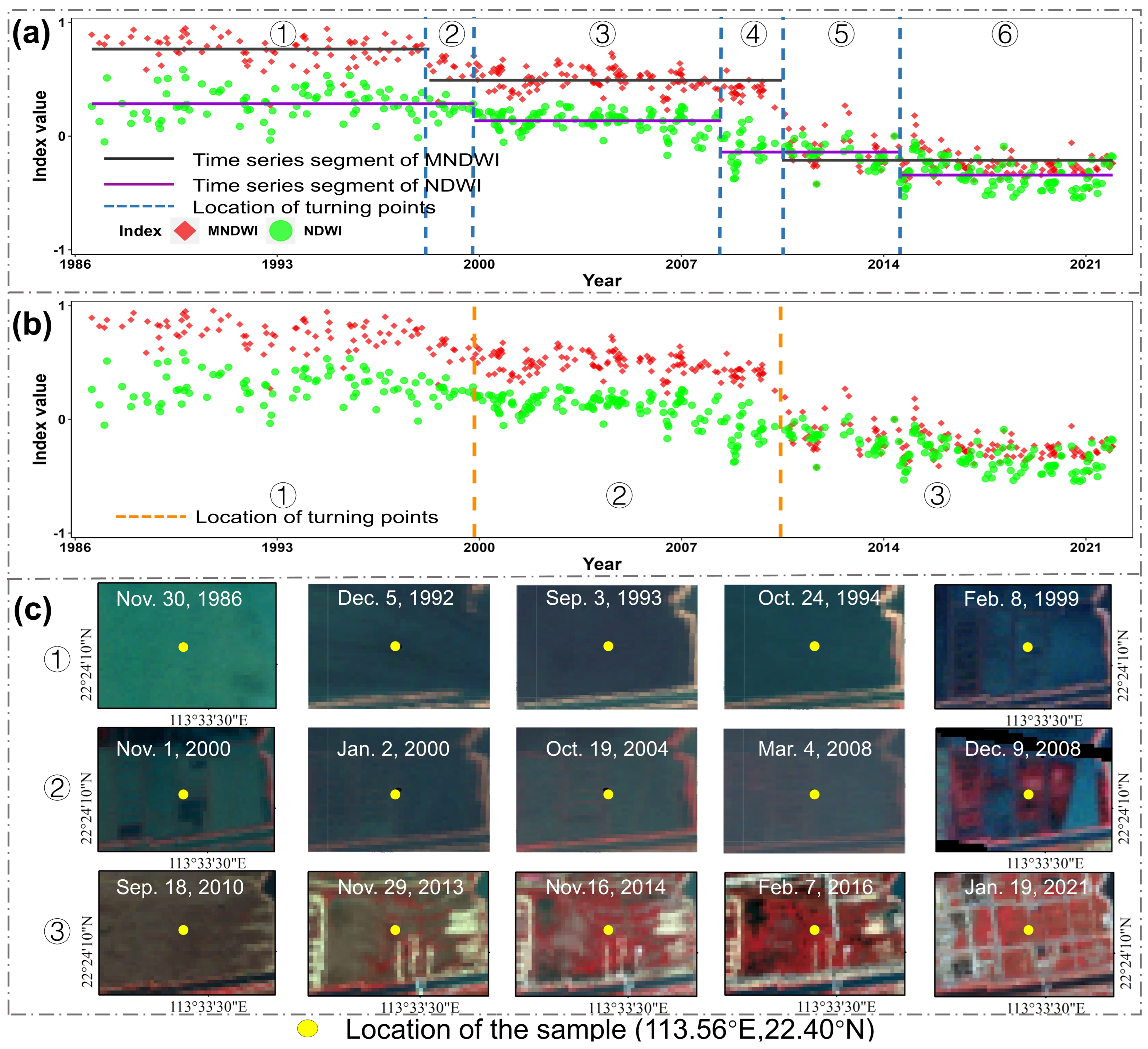
3.2. Spectra Feature Analysis
3.3. Time Series Segmentation
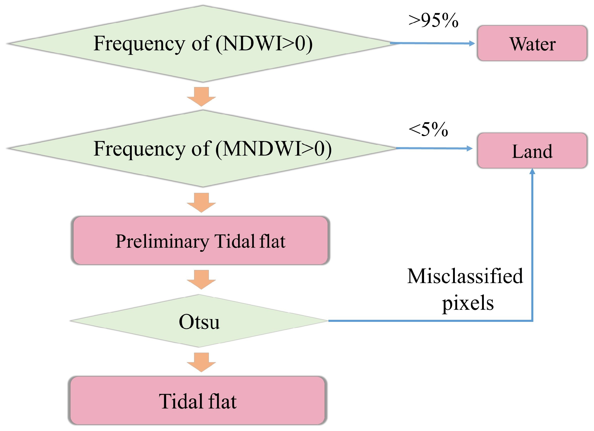
3.4. Tide-Independent Hierarchical Classification Strategy
3.5. Accuracy Assessment Strategy
4. Results
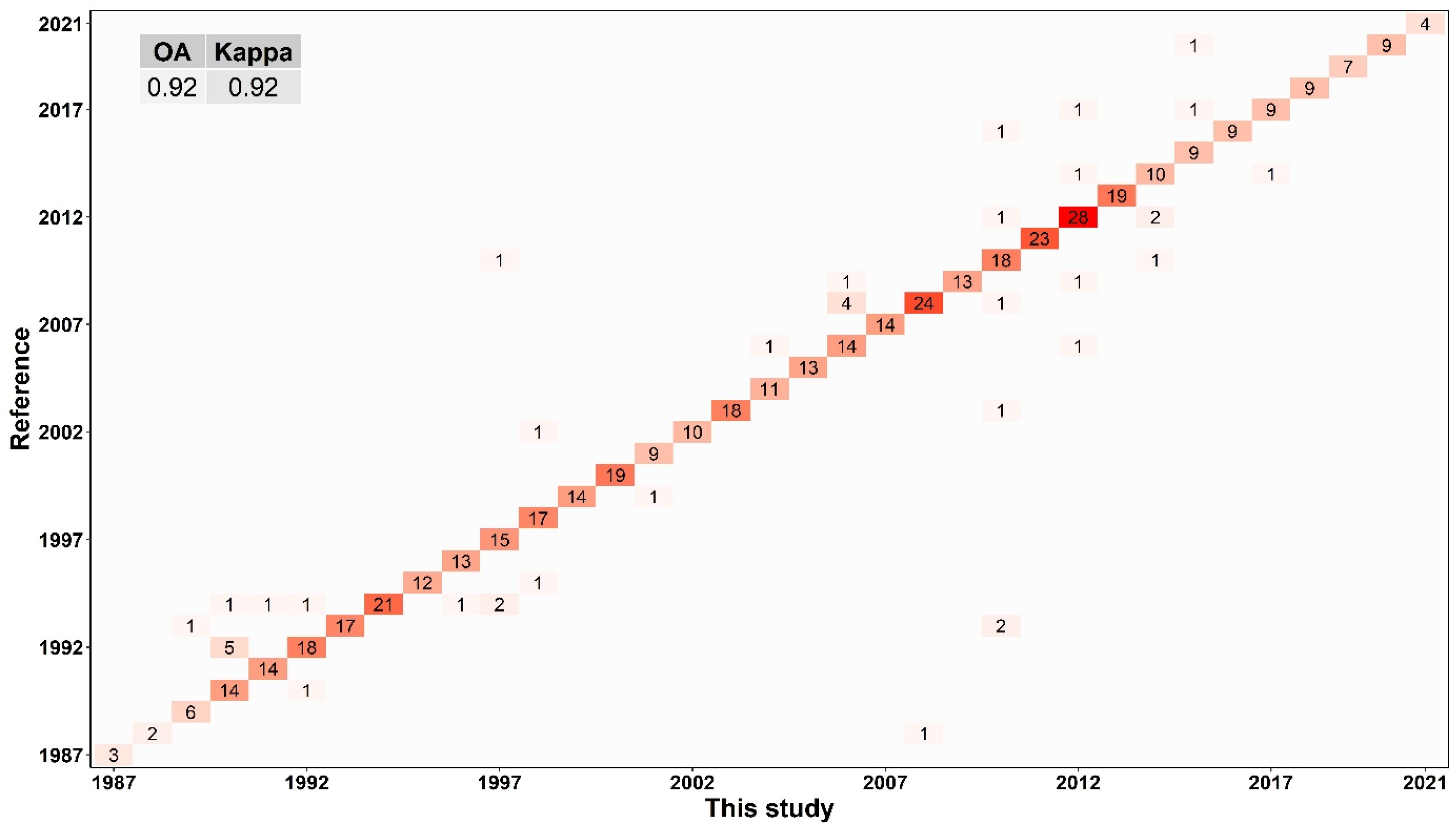
4.1. Accuracy of Annual Tidal Flats
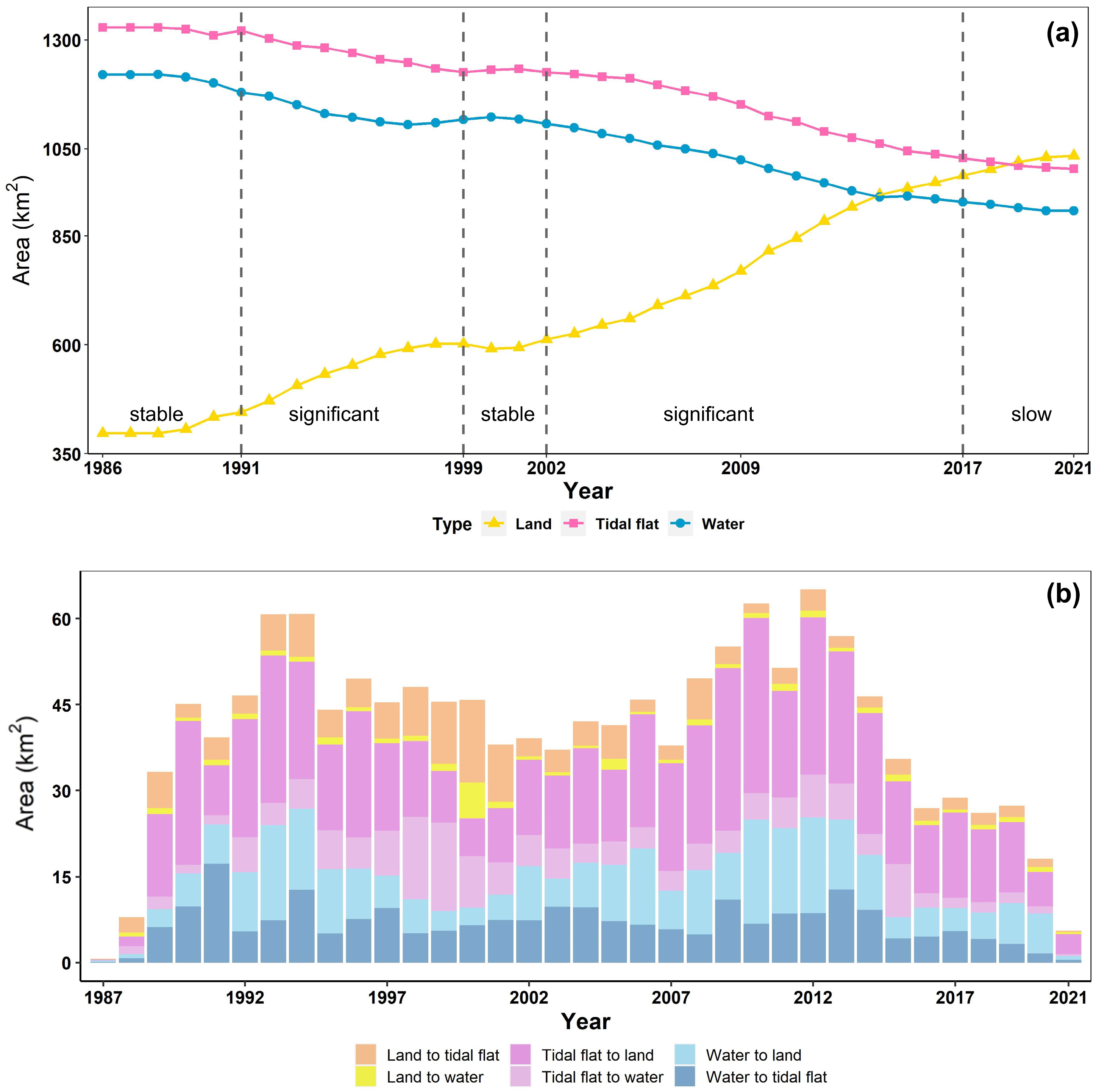
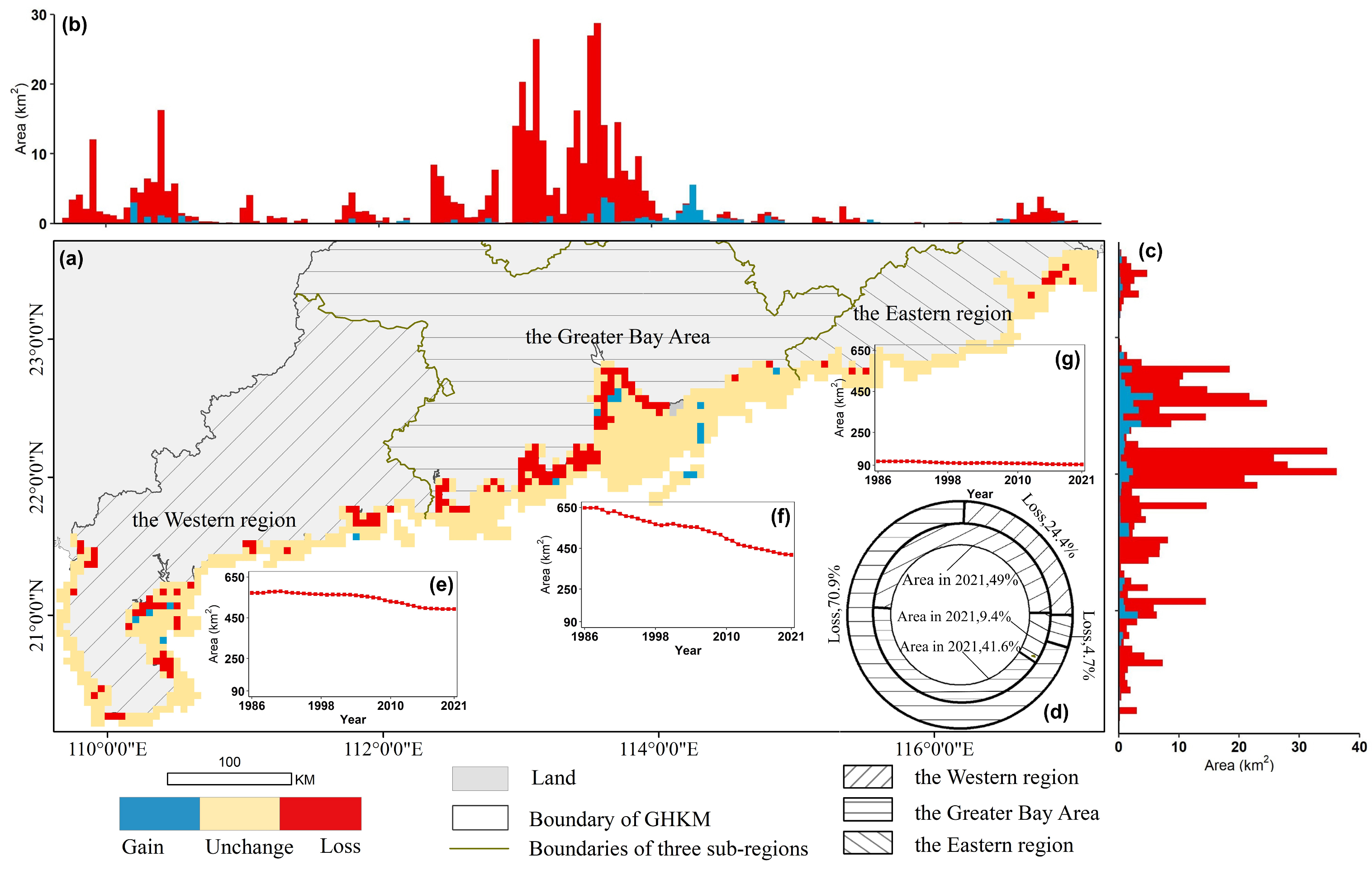
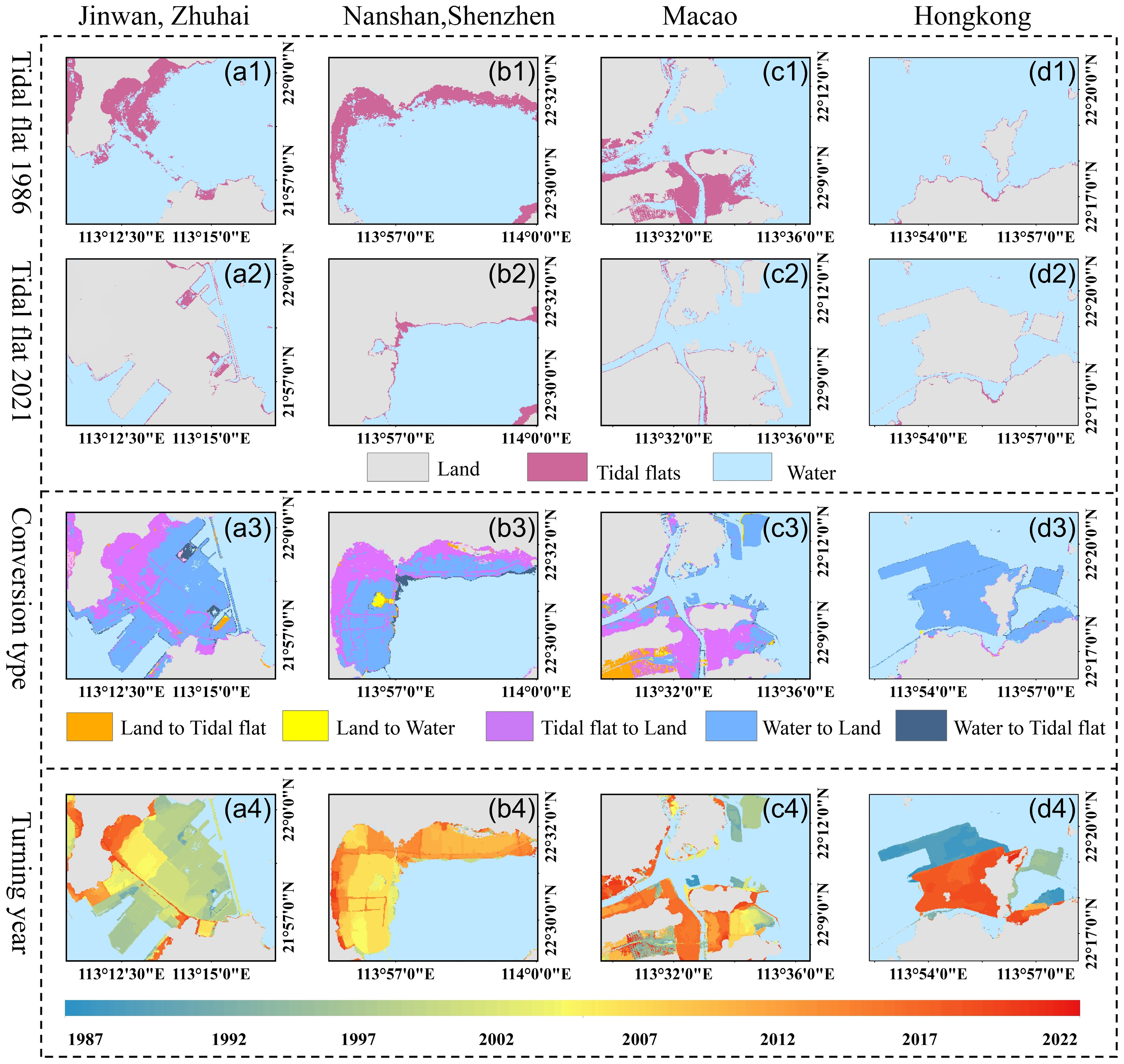
4.2. Annual Loss and Gain Dynamics of Tidal Flats
4.3. Policy Drivers for the Tidal Flat Dynamics
5. Discussion
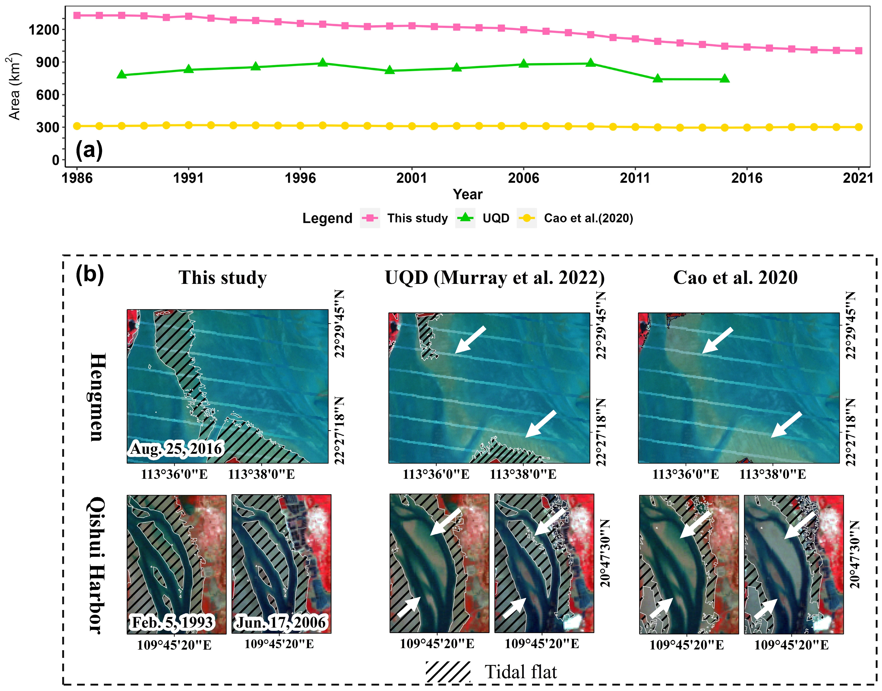
5.1. Mapping Performances Compared with Other Methods
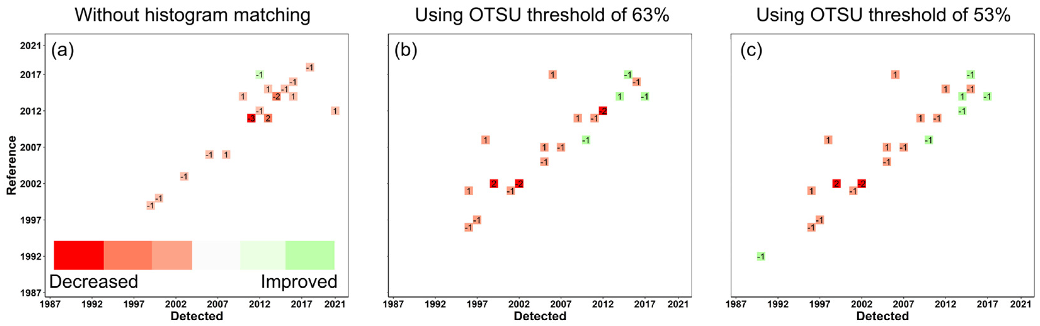
5.2. Sensitivity Analysis of the Method
6. Conclusions
Author Contributions
Funding
Data Availability Statement
Acknowledgments
Conflicts of Interest
References
- Dyer, K.R.; Christie, M.C.; Wright, E.W. The classification of intertidal mudflats. Cont. Shelf Res. 2000, 20, 1039–1060. [Google Scholar] [CrossRef]
- Barbier, E.B.; Hacker, S.D.; Kennedy, C.; Koch, E.W.; Stier, A.C.; Silliman, B.R. The value of estuarine and coastal ecosystem services. Ecol. Monogr. 2011, 81, 169–193. [Google Scholar] [CrossRef]
- Madhuanand, L.; Philippart, C.J.M.; Wang, J.; Nijland, W.; de Jong, S.M.; Bijleveld, A.I.; Addink, E.A. Enhancing the predictive performance of remote sensing for ecological variables of tidal flats using encoded features from a deep learning model. GIScience Remote Sens. 2023, 60, 2163048. [Google Scholar] [CrossRef]
- Murray, N.J.; Clemens, R.S.; Phinn, S.R.; Possingham, H.P.; Fuller, R.A. Tracking the rapid loss of tidal wetlands in the Yellow Sea. Front. Ecol. Environ. 2014, 12, 267–272. [Google Scholar] [CrossRef] [PubMed]
- Wang, Y.; Liu, Y.; Jin, S.; Sun, C.; Wei, X. Evolution of the topography of tidal flats and sandbanks along the Jiangsu coast from 1973 to 2016 observed from satellites. ISPRS J. Photogramm. Remote Sens. 2019, 150, 27–43. [Google Scholar] [CrossRef]
- Shi, J.; Feng, X.; Toumi, R.; Zhang, C.; Hodges, K.I.; Tao, A.; Zhang, W.; Zheng, J. Global increase in tropical cyclone ocean surface waves. Nat. Commun. 2024, 15, 174. [Google Scholar] [CrossRef] [PubMed]
- Murray, N.J.; Ma, Z.; Fuller, R.A. Tidal flats of the Yellow Sea: A review of ecosystem status and anthropogenic threats. Austral Ecol. 2015, 40, 472–481. [Google Scholar] [CrossRef]
- Cao, W.; Zhou, Y.; Li, R.; Li, X. Mapping changes in coastlines and tidal flats in developing islands using the full time series of Landsat images. Remote Sens. Environ. 2020, 239, 111665. [Google Scholar] [CrossRef]
- Gibson, R.; Atkinson, R.; Gordon, J. Loss, status and trends for coastal marine habitats of Europe. Oceanogr. Mar. Biol. Annu. Rev. 2007, 45, 345–405. [Google Scholar]
- Liu, Y.; Li, J.; Sun, C.; Wang, X.; Tian, P.; Chen, L.; Zhang, H.; Yang, X.; He, G. Thirty-year changes of the coastlines, wetlands, and ecosystem services in the Asia major deltas. J. Environ. Manag. 2023, 326, 116675. [Google Scholar] [CrossRef]
- Tong, S.S.; Deroin, J.P.; Pham, T.L. An optimal waterline approach for studying tidal flat morphological changes using remote sensing data: A case of the northern coast of Vietnam. Estuar. Coast. Shelf Sci. 2020, 236, 106613. [Google Scholar] [CrossRef]
- Wang, X.; Xiao, X.; Zou, Z.; Chen, B.; Ma, J.; Dong, J.; Doughty, R.B.; Zhong, Q.; Qin, Y.; Dai, S.; et al. Tracking annual changes of coastal tidal flats in China during 1986–2016 through analyses of Landsat images with Google Earth Engine. Remote Sens. Environ. 2020, 238, 110987. [Google Scholar] [CrossRef] [PubMed]
- Ghosh, S.; Mishra, D.R.; Gitelson, A.A. Long-term monitoring of biophysical characteristics of tidal wetlands in the northern Gulf of Mexico—A methodological approach using MODIS. Remote Sens. Environ. 2016, 173, 39–58. [Google Scholar] [CrossRef]
- Wu, W.; Zhi, C.; Gao, Y.; Chen, C.; Chen, Z.; Su, H.; Lu, W.; Tian, B. Increasing fragmentation and squeezing of coastal wetlands: Status, drivers, and sustainable protection from the perspective of remote sensing. Sci. Total Environ. 2022, 811, 152339. [Google Scholar] [CrossRef]
- Zhang, H.; Li, D.; Wang, J.; Zhou, H.; Guan, W.; Lou, X.; Cao, W.; Shi, A.; Chen, P.; Fan, K.; et al. Long time-series remote sensing analysis of the periodic cycle evolution of the inlets and ebb-tidal delta of Xincun Lagoon, Hainan Island, China. ISPRS J. Photogramm. Remote Sens. 2020, 165, 67–85. [Google Scholar] [CrossRef]
- Song, S.; Wu, Z.; Wang, Y.; Cao, Z.; He, Z.; Su, Y. Mapping the Rapid Decline of the Intertidal Wetlands of China Over the Past Half Century Based on Remote Sensing. Front. Earth Sci. 2020, 8, 16. [Google Scholar] [CrossRef]
- Yan, J.; Zhao, S.; Su, F.; Du, J.; Feng, P.; Zhang, S. Tidal Flat Extraction and Change Analysis Based on the RF-W Model: A Case Study of Jiaozhou Bay, East China. Remote Sens. 2021, 13, 1436. [Google Scholar] [CrossRef]
- Yang, W.; Sha, J.; Bao, Z.; Dong, J.; Li, X.; Shifaw, E.; Tan, J.; Sodango, T.H. Monitoring tidal flats boundaries through combining Sentinel-1 and Sentinel-2 imagery. Environ. Technol. Innov. 2021, 22, 101401. [Google Scholar] [CrossRef]
- Zhang, K.; Dong, X.; Liu, Z.; Gao, W.; Hu, Z.; Wu, G. Mapping Tidal Flats with Landsat 8 Images and Google Earth Engine: A Case Study of the China’s Eastern Coastal Zone circa 2015. Remote Sens. 2019, 11, 924. [Google Scholar] [CrossRef]
- Xu, C.; Liu, W. Mapping and analyzing the annual dynamics of tidal flats in the conterminous United States from 1984 to 2020 using Google Earth Engine. Environ. Adv. 2022, 7, 100147. [Google Scholar] [CrossRef]
- Chen, Y.; Dong, J.; Xiao, X.; Zhang, M.; Tian, B.; Zhou, Y.; Li, B.; Ma, Z. Land claim and loss of tidal flats in the Yangtze Estuary. Sci. Rep. 2016, 6, 24018. [Google Scholar] [CrossRef]
- Li, W.; Gong, P. Continuous monitoring of coastline dynamics in western Florida with a 30-year time series of Landsat imagery. Remote Sens. Environ. 2016, 179, 196–209. [Google Scholar] [CrossRef]
- Sagar, S.; Roberts, D.; Bala, B.; Lymburner, L. Extracting the intertidal extent and topography of the Australian coastline from a 28year time series of Landsat observations. Remote Sens. Environ. 2017, 195, 153–169. [Google Scholar] [CrossRef]
- Tseng, K.-H.; Kuo, C.-Y.; Lin, T.-H.; Huang, Z.-C.; Lin, Y.-C.; Liao, W.-H.; Chen, C.-F. Reconstruction of time-varying tidal flat topography using optical remote sensing imageries. ISPRS J. Photogramm. Remote Sens. 2017, 131, 92–103. [Google Scholar] [CrossRef]
- Wang, X.; Yan, F.; Su, F. Impacts of urbanization on the ecosystem services in the Guangdong-Hong Kong-Macao Greater Bay Area, China. Remote Sens. 2020, 12, 3269. [Google Scholar] [CrossRef]
- Murray, N.J.; Phinn, S.P.; Fuller, R.A.; DeWitt, M.; Ferrari, R.; Johnston, R.; Clinton, N.; Lyons, M.B. High-resolution global maps of tidal flat ecosystems from 1984 to 2019. Sci. Data 2022, 9, 542. [Google Scholar] [CrossRef]
- Murray, N.J.; Phinn, S.R.; DeWitt, M.; Ferrari, R.; Johnston, R.; Lyons, M.B.; Clinton, N.; Thau, D.; Fuller, R.A. The global distribution and trajectory of tidal flats. Nature 2019, 565, 222–225. [Google Scholar] [CrossRef] [PubMed]
- Zhang, X.; Liu, L.; Wang, J.; Zhao, T.; Liu, W.; Chen, X. Automated Mapping of Global 30-m Tidal Flats Using Time-Series Landsat Imagery: Algorithm and Products. J. Remote Sens. 2023, 3, 0091. [Google Scholar] [CrossRef]
- Davies, J.L.; Davies, J.L.; Davies, J.; Gideon, J.D.; Davies, L.; Davies, M.C. A morphogenic approach to world shorelines. Z. Geomorphol. 1964, 8, 127–142. [Google Scholar] [CrossRef]
- Daidu, F.; Yuan, W.; Min, L. Classifications, sedimentary features and facies associations of tidal flats. J. Palaeogeogr. 2013, 2, 66–80. [Google Scholar] [CrossRef]
- Wang, Y.; Zhu, D. Modern coral reefs in the South China Sea. In Oceanology of China Sea; Zhou, D., Liang, Y., Zeng, C.K., Eds.; Kluwer Academic Publ.: Norwell, MA, USA, 1994; Volume 2, pp. 445–456. [Google Scholar]
- Chen, B.; Xiao, X.; Li, X.; Pan, L.; Doughty, R.; Ma, J.; Dong, J.; Qin, Y.; Zhao, B.; Wu, Z.; et al. A mangrove forest map of China in 2015: Analysis of time series Landsat 7/8 and Sentinel-1A imagery in Google Earth Engine cloud computing platform. ISPRS J. Photogramm. Remote Sens. 2017, 131, 104–120. [Google Scholar] [CrossRef]
- Guo, H.; Cai, Y.; Yang, Z.; Zhu, Z.; Ouyang, Y. Dynamic simulation of coastal wetlands for Guangdong-Hong Kong-Macao Greater Bay area based on multi-temporal Landsat images and FLUS model. Ecol. Indic. 2021, 125, 107559. [Google Scholar] [CrossRef]
- Li, L.; Wang, Y. Land use/cover change from 2001 to 2010 and its socioeconomic determinants in Guangdong Province, a rapid urbanization area of China. Tarım Bilim. Derg. 2016, 22, 275–294. [Google Scholar] [CrossRef]
- Ma, C.; Ai, B.; Zhao, J.; Xu, X.; Huang, W. Change Detection of Mangrove Forests in Coastal Guangdong during the Past Three Decades Based on Remote Sensing Data. Remote Sens. 2019, 11, 921. [Google Scholar] [CrossRef]
- Hasan, S.; Shi, W.; Zhu, X.; Abbas, S. Monitoring of Land Use/Land Cover and Socioeconomic Changes in South China over the Last Three Decades Using Landsat and Nighttime Light Data. Remote Sens. 2019, 11, 1658. [Google Scholar] [CrossRef]
- National Bureau of Statistics of China. China Statistical Yearbook. 2022. Available online: https://www.stats.gov.cn/sj/ndsj/2022/indexeh.htm (accessed on 5 January 2023).
- Chen, Y.; Li, X.; Liu, X.; Ai, B. Analyzing land-cover change and corresponding impacts on carbon budget in a fast developing sub-tropical region by integrating MODIS and Landsat TM/ETM+ images. Appl. Geogr. 2013, 45, 10–21. [Google Scholar] [CrossRef]
- Hasan, S.; Shi, W.; Zhu, X. Impact of land use land cover changes on ecosystem service value—A case study of Guangdong, Hong Kong, and Macao in South China. PLoS ONE 2020, 15, e0231259. [Google Scholar] [CrossRef]
- He, H.; Miao, H.; Liang, Z.; Zhang, Y.; Jiang, W.; Deng, Z.; Tang, J.; Liu, G.; Luo, X. Prevalence of small for gestational age infants in 21 cities in China, 2014–2019. Sci. Rep. 2021, 11, 7500. [Google Scholar] [CrossRef] [PubMed]
- Li, F.; Jupp, D.L.; Thankappan, M.; Lymburner, L.; Mueller, N.; Lewis, A.; Held, A. A physics-based atmospheric and BRDF correction for Landsat data over mountainous terrain. Remote Sens. Environ. 2012, 124, 756–770. [Google Scholar] [CrossRef]
- Loveland, T.R.; Dwyer, J.L. Landsat: Building a strong future. Remote Sens. Environ. 2012, 122, 22–29. [Google Scholar] [CrossRef]
- Masek, J.G.; Vermote, E.F.; Saleous, N.E.; Wolfe, R.; Hall, F.G.; Huemmrich, K.F.; Feng, G.; Kutler, J.; Teng-Kui, L. A Landsat surface reflectance dataset for North America, 1990–2000. IEEE Geosci. Remote Sens. Lett. 2006, 3, 68–72. [Google Scholar] [CrossRef]
- Zhu, Z.; Woodcock, C.E. Object-based cloud and cloud shadow detection in Landsat imagery. Remote Sens. Environ. 2012, 118, 83–94. [Google Scholar] [CrossRef]
- Roy, D.P.; Kovalskyy, V.; Zhang, H.; Vermote, E.F.; Yan, L.; Kumar, S.; Egorov, A. Characterization of Landsat-7 to Landsat-8 reflective wavelength and normalized difference vegetation index continuity. Remote Sens. Environ. 2016, 185, 57–70. [Google Scholar] [CrossRef]
- Foga, S.; Scaramuzza, P.L.; Guo, S.; Zhu, Z.; Dilley, R.D.; Beckmann, T.; Schmidt, G.L.; Dwyer, J.L.; Hughes, M.J.; Laue, B. Cloud detection algorithm comparison and validation for operational Landsat data products. Remote Sens. Environ. 2017, 194, 379–390. [Google Scholar] [CrossRef]
- McFeeters, S.K. The use of the Normalized Difference Water Index (NDWI) in the delineation of open water features. Int. J. Remote Sens. 1996, 17, 1425–1432. [Google Scholar] [CrossRef]
- Xu, H. Modification of normalised difference water index (NDWI) to enhance open water features in remotely sensed imagery. Int. J. Remote Sens. 2006, 27, 3025–3033. [Google Scholar] [CrossRef]
- Xiao, X.; Boles, S.; Frolking, S.; Salas, W.; Moore, B.; Li, C.; He, L.; Zhao, R. Observation of flooding and rice transplanting of paddy rice fields at the site to landscape scales in China using VEGETATION sensor data. Int. J. Remote Sens. 2002, 23, 3009–3022. [Google Scholar] [CrossRef]
- Feyisa, G.L.; Meilby, H.; Fensholt, R.; Proud, S.R. Automated Water Extraction Index: A new technique for surface water mapping using Landsat imagery. Remote Sens. Environ. 2014, 140, 23–35. [Google Scholar] [CrossRef]
- Acharya, T.D.; Subedi, A.; Lee, D.H. Evaluation of Water Indices for Surface Water Extraction in a Landsat 8 Scene of Nepal. Sensors 2018, 18, 2580. [Google Scholar] [CrossRef]
- Fisher, A.; Flood, N.; Danaher, T. Comparing Landsat water index methods for automated water classification in eastern Australia. Remote Sens. Environ. 2016, 175, 167–182. [Google Scholar] [CrossRef]
- Scott, A.J.; Knott, M. A cluster analysis method for grouping means in the analysis of variance. Biometrics 1974, 30, 507–512. [Google Scholar] [CrossRef]
- Sen, A.; Srivastava, M.S. On tests for detecting change in mean. Ann. Stat. 1975, 3, 98–108. [Google Scholar] [CrossRef]
- Otsu, N. A Threshold Selection Method from Gray-Level Histograms. IEEE Trans. Syst. Man Cybern. 1979, 9, 62–66. [Google Scholar] [CrossRef]
- Ren, C.; Wang, Z.; Zhang, Y.; Zhang, B.; Chen, L.; Xi, Y.; Xiao, X.; Doughty, R.B.; Liu, M.; Jia, M.; et al. Rapid expansion of coastal aquaculture ponds in China from Landsat observations during 1984–2016. Int. J. Appl. Earth Obs. Geoinf. 2019, 82, 101902. [Google Scholar] [CrossRef]
- Ai, B.; Huang, K.; Zhao, J.; Sun, S.; Jian, Z.; Liu, X. Comparison of classification algorithms for detecting typical coastal reclamation in Guangdong Province with Landsat 8 and Sentinel 2 Images. Remote Sens. 2022, 14, 385. [Google Scholar] [CrossRef]
- Feng, T.; Xu, N. Satellite-based monitoring of annual coastal reclamation in Shenzhen and Hong Kong since the 21st Century: A comparative study. J. Mar. Sci. Eng. 2021, 9, 48. [Google Scholar] [CrossRef]
- Yan-hong, Y.; Cong, Y. The reasons, development and problems of the land reclamation. Chin. J. Nat. 2014, 36, 437–444. [Google Scholar]
- Duan, Y.; Tian, B.; Li, X.; Liu, D.; Sengupta, D.; Wang, Y.; Peng, Y. Tracking changes in aquaculture ponds on the China coast using 30 years of Landsat images. Int. J. Appl. Earth Obs. Geoinf. 2021, 102, 102383. [Google Scholar] [CrossRef]
- Li, L.Y.; Qi, Z.X.; Xian, S. Decoding spatiotemporal patterns of urban land sprawl in Zhuhai, China. Appl. Ecol. Environ. Res. 2020, 18, 913–927. [Google Scholar] [CrossRef]
- Miao, D.; Xue, Z. The current developments and impact of land reclamation control in China. Mar. Policy 2021, 134, 104782. [Google Scholar] [CrossRef]
- Jiang, X.-Z.; Liu, T.-Y.; Su, C.-W. China’s marine economy and regional development. Mar. Policy 2014, 50, 227–237. [Google Scholar] [CrossRef]


| a (1986) | Reference | ||||||||||||
| Land | Tidal flat | Water | UA | ||||||||||
| Classification | Land | 194 | 4 | 2 | 97% | ||||||||
| Tidal flat | 4 | 177 | 19 | 89% | |||||||||
| Water | 0 | 2 | 198 | 99% | |||||||||
| PA | 98% | 97% | 90% | ||||||||||
| OA | 95% | Kappa | 0.92 | ||||||||||
| b (2021) | Reference | ||||||||||||
| Land | Tidal flat | Water | UA | ||||||||||
| Classification | Land | 194 | 6 | 0 | 97% | ||||||||
| Tidal flat | 6 | 171 | 23 | 86% | |||||||||
| Water | 1 | 6 | 193 | 97% | |||||||||
| PA | 97% | 93% | 89% | ||||||||||
| OA | 93% | Kappa | 0.90 | ||||||||||
| c (Conversion types) | Reference | ||||||||||||
| Classification | Land to Tidal flat | Land to Water | Tidal flat to Land | Tidal flat to Water | Water to Land | Water to Tidal flat | Unchanged | ||||||
| Land to Tidal flat | 29 | 5 | 0 | 0 | 0 | 0 | 4 | ||||||
| Land to Water | 1 | 19 | 0 | 3 | 0 | 0 | 0 | ||||||
| Tidal flat to Land | 0 | 0 | 187 | 0 | 6 | 0 | 10 | ||||||
| Tidal flat to Water | 0 | 1 | 0 | 67 | 0 | 0 | 15 | ||||||
| Water to Land | 0 | 0 | 0 | 0 | 104 | 1 | 0 | ||||||
| Water to Tidal flat | 0 | 0 | 0 | 0 | 1 | 78 | 11 | ||||||
| Unchanged | 0 | 0 | 0 | 0 | 0 | 0 | 11 | ||||||
| OA | 89% | Kappa | 0.86 | ||||||||||
| OA of Conversion Types | OA of Turning Years | |
|---|---|---|
| This study | 89% | 92% |
| Without histogram matching | 86% | 91% |
| Using the OSTU threshold of 63% | 88% | 91% |
| Using the OSTU threshold of 53% | 88% | 91% |
| Without Histogram Matching | Reference | ||||||
|---|---|---|---|---|---|---|---|
| Classification | Land to Tidal flat | Land to Water | Tidal flat to Land | Tidal flat to Water | Water to Land | Water to Tidal flat | Unchanged |
| Land to Tidal flat | 4 (−1) | 0 | 0 | 0 | 0 | 0 | 0 |
| Land to Water | 1 (+1) | 2 | 0 | 1 | 0 | 0 | 0 |
| Tidal flat to Land | 0 | 0 | 41 (−1) | 0 | 1 | 0 | 3 (+1) |
| Tidal flat to Water | 0 | 0 | 0 | 11 (+1) | 0 | 0 | 6 (+4) |
| Water to Land | 0 | 0 | 1 (+1) | 0 | 20 | 0 | 0 |
| Water to Tidal flat | 0 | 0 | 0 | 0 | 0 | 9 | 2 |
| Unchanged | 0 | 0 | 0 | 0 (−1) | 0 | 0 | 0 (−5) |
| OA | 86% | ||||||
| (a) Using Otsu threshold of 63% | Reference | ||||||
| Classification | Land to Tidal flat | Land to Water | Tidal flat to Land | Tidal flat to Water | Water to Land | Water to Tidal flat | Unchanged |
| Land to Tidal flat | 29 | 5 | 0 | 0 | 0 | 0 | 41 |
| Land to Water | 1 | 19 | 0 | 4 (+1) | 0 | 0 | 0 |
| Tidal flat to Land | 0 | 0 | 183 (−4) | 0 | 6 | 0 | 10 |
| Tidal flat to Water | 0 | 1 | 0 | 66 (−1) | 0 | 0 | 15 |
| Water to Land | 0 | 0 | 3 | 0 | 104 | 4 (+3) | 0 |
| Water to Tidal flat | 0 | 0 | 0 | 0 | 1 | 75 (−3) | 11 |
| Unchanged | 0 | 0 | 4 (+4) | 0 | 0 | 0 | 11 |
| OA | 88% | ||||||
| (b) Using Otsu threshold of 53% | Reference | ||||||
| Classification | Land to Tidal flat | Land to Water | Tidal flat to Land | Tidal flat to Water | Water to Land | Water to Tidal flat | Unchanged |
| Land to Tidal flat | 29 | 5 | 0 | 0 | 0 | 0 | 4 |
| Land to Water | 1 | 19 | 0 | 4 (+1) | 0 | 0 | 0 |
| Tidal flat to Land | 0 | 0 | 183 (−4) | 0 | 6 | 0 | 10 |
| Tidal flat to Water | 0 | 1 | 0 | 66 (−1) | 0 | 0 | 15 |
| Water to Land | 0 | 0 | 3 | 0 | 104 | 1 | 0 |
| Water to Tidal flat | 0 | 0 | 0 | 0 | 1 | 78 | 11 |
| Unchanged | 0 | 0 | 4 (+4) | 0 | 0 | 0 | 11 |
| OA | 88% | ||||||
Disclaimer/Publisher’s Note: The statements, opinions and data contained in all publications are solely those of the individual author(s) and contributor(s) and not of MDPI and/or the editor(s). MDPI and/or the editor(s) disclaim responsibility for any injury to people or property resulting from any ideas, methods, instructions or products referred to in the content. |
© 2024 by the authors. Licensee MDPI, Basel, Switzerland. This article is an open access article distributed under the terms and conditions of the Creative Commons Attribution (CC BY) license (https://creativecommons.org/licenses/by/4.0/).
Share and Cite
Luo, J.; Cao, W.; Li, X.; Zhou, Y.; He, S.; Zhang, Z.; Li, D.; Zhang, H. Mapping Annual Tidal Flat Loss and Gain in the Micro-Tidal Area Integrating Dual Full-Time Series Spectral Indices. Remote Sens. 2024, 16, 1402. https://doi.org/10.3390/rs16081402
Luo J, Cao W, Li X, Zhou Y, He S, Zhang Z, Li D, Zhang H. Mapping Annual Tidal Flat Loss and Gain in the Micro-Tidal Area Integrating Dual Full-Time Series Spectral Indices. Remote Sensing. 2024; 16(8):1402. https://doi.org/10.3390/rs16081402
Chicago/Turabian StyleLuo, Jiayi, Wenting Cao, Xuecao Li, Yuyu Zhou, Shuangyan He, Zhaoyuan Zhang, Dongling Li, and Huaguo Zhang. 2024. "Mapping Annual Tidal Flat Loss and Gain in the Micro-Tidal Area Integrating Dual Full-Time Series Spectral Indices" Remote Sensing 16, no. 8: 1402. https://doi.org/10.3390/rs16081402
APA StyleLuo, J., Cao, W., Li, X., Zhou, Y., He, S., Zhang, Z., Li, D., & Zhang, H. (2024). Mapping Annual Tidal Flat Loss and Gain in the Micro-Tidal Area Integrating Dual Full-Time Series Spectral Indices. Remote Sensing, 16(8), 1402. https://doi.org/10.3390/rs16081402