Exploring the Effects of Topography on Leaf Area Index Retrieved from Remote Sensing Data at Various Spatial Scales over Rugged Terrains

Abstract

Topography significantly affects remotely sensed reflectance data and subsequently impacts the retrieval of the leaf area index (LAI) from surface reflectance data over rugged terrains. However, most LAI inversion algorithms ignore the influence of terrain. This paper quantitatively analyzes the topographic effects on LAI values retrieved from remote sensing data at various spatial scales (30, 90, 270, 540, 1080, and 5400 m) over rugged terrains. The PRO4SAILT (PROSPECT + 4SAILT) model and the Proy algorithm were used to simulate multiscale surface reflectance for different LAI values over rugged terrains. Based on Gaussian process regression (GPR), an LAI inversion algorithm that ignores terrain effects was first developed. The simulated multiscale reflectance data were subsequently input into the inversion algorithm to retrieve LAI values. Finally, the retrieved LAI values were compared with the corresponding reference LAI values. The results demonstrate that the finer the spatial resolution is, the more significant the topographic effects on the retrieved LAI values are. When the reference LAI is five, as the spatial resolution increases from 5400 m to 30 m, the mean percentage error (MPE) of the retrieved LAI increases from 10.46% to 13.72%, and the root mean square error (RMSE) increases from 0.5376 to 1.005. Regardless of the spatial resolution, the error in the retrieved LAI values increases with an increasing terrain slope. When the reference LAI is five and the spatial resolution is 30 m, the MPE at a slope of 15°–30° is close to 5%, and the RMSE is close to 0.3. The MPE at a slope of 30°–45° is close to 20%, and the RMSE is close to one. In addition, the accuracy of the retrieved LAI values is closely related to the sky view factor (SVF). In general, the larger the SVF is, the smaller the error in the retrieved LAI values. In addition, the conversion relationships between the retrieved LAI values using the algorithm that ignores terrain effects and the true LAI values are provided in this study.

1. Introduction

The leaf area index (LAI) is an important structural parameter that plays a crucial role in vegetation growth monitoring [1] and global climate change [2]. It is defined as the total one-sided surface area of all green leaves in the canopy [3]. Many methods, including empirical methods and physical model-based methods, have been developed to retrieve LAI values from remote sensing data.

In recent years, machine learning methods such as the artificial neural network (ANN) and Gaussian process regression (GPR) methods have been increasingly applied to retrieve LAI values from remote sensing data [4,5,6,7,8,9,10,11]. Xiao et al. [5] applied generalized regression neural networks (GRNNs) to retrieve LAI values from time series of Moderate Resolution Imaging Spectroradiometer (MODIS) and Advanced Very-High-Resolution Radiometer (AVHRR) surface reflectance data. Gewali et al. [10] successfully estimated canopy structural and biochemical parameters from hyperspectral data using the GPR model. ESTEVEZ et al. [11] developed an algorithm for retrieving LAI values from Sentinel-2 Top of Atmosphere (TOA) radiation data using the GPR method and achieved good accuracy. Adeluyi et al. [12] estimated the phenological dynamics of irrigated rice LAI values using a combination of the PROSAIL model and the GPR model, and the results were significantly better than the S2ToolBox Level 2 LAI results obtained via a combination of the PROSAIL model and an ANN.

Over the past two decades, many regional and global LAI products with low to medium spatial resolutions, such as the MODIS [13], CYCLOPES [4], GEOV1 [6], and Global Land Surface Satellite (GLASS) [5] LAI products, have been generated from satellite remote sensing data. These LAI products have played a crucial role in studies of climate change [14,15,16], carbon cycling [17,18], vegetation phenology [19,20], and land use change [21]. However, most of the current methods used to generate low- and medium-spatial-resolution LAI products assume a horizontal surface and ignore the influence of topographic effects. Therefore, the quality requirements of the Global Climate Observing System (GCOS) for LAI corresponding to the maximum values of relative accuracy (20%) and uncertainty (0.5) are difficult to satisfy over rugged surfaces [22]. This hinders further applications of these LAI products, such as land surface modeling, precision agriculture [23,24,25], forest mapping [26], and urban research [27,28], which require high-quality LAI data.

The topography changes the incoming and outgoing radiation of targeted pixels in three ways: (1) the topography alters sun-target-sensor geometries, thereby changing the direct radiation received by each pixel; (2) the incoming (from the sky) and outgoing diffuse irradiance from a pixel differ from those over horizontal surfaces due to the obstruction of the surrounding topography; and (3) the radiation reflected/emitted from adjacent pixels to a target pixel is another source of diffuse radiation, referred to as terrain radiation [29]. Moreover, the geotropic growth of vegetation on slopes can lead to the characterization of the vegetation scattering medium not as a direct coordinate rotation but rather in relation to the path length of the light path [30].

Several studies have demonstrated that ignoring topography induces errors in LAI estimation. Gonsamo et al. [31] reported that LAI values inverted by considering and ignoring the influence of topographic factors significantly differed over rugged terrains. Jin et al. [22] reported that the spatial and temporal integrity and accuracy of the MODIS and GLASS LAI products are significantly lower in high-elevation and high-terrain relief areas than in horizontal terrain areas. Mousivand et al. [29] reported that ignoring terrain effects could result in an LAI inversion error of more than 0.5. Based on simulation data from the DART model, Yu et al. [32] compared the accuracy of LAI inversion on horizontal surfaces and sloped surfaces and reported that the mean absolute error (MAE) of LAI inversion on horizontal surfaces was 0.15 while the error of the LAI inversion on sloped surfaces increased significantly with an increasing slope, and the inversion error reached 51% on average when the slope reached 60°. The above studies have directly or indirectly shown that topography plays an important role in the processing of low- and medium-spatial-resolution data [33,34,35,36].

However, there are still several challenges and limitations in the existing research on the topographic effects of LAI inversion over rugged terrains, and additional research is needed for further discussion. First, most of the current research has focused on a single spatial resolution rather than on different spatial resolutions; moreover, these approaches cannot meet the requirements of multiscale mountain LAI research and are not conducive to the construction of corresponding mountain LAI inversion algorithms. In addition, most of the studies have generally analyzed low-spatial-resolution LAI products, and few studies have analyzed topographic effects in high-spatial-resolution LAI inversion. Moreover, a comprehensive analysis of multiple topographical variables is needed instead of focusing on a single factor.

This study aimed to explore the topographic effects on LAI estimation at various spatial scales over rugged terrains. The LAI inversion error caused by ignoring topographic effects at different spatial scales was analyzed based on simulated multiscale surface reflectance over rugged terrains. First, the reflectance over rugged terrains at different spatial scales (30, 90, 270, 540, 1080, and 5400 m) were simulated, input into an LAI inversion model ignoring terrain effects based on the GPR method, and then inverted to obtain the biased LAI. The root mean square error (RMSE) and mean error percentage (MEP) were used to quantify the error from the perspectives of single factor analysis of the slope and sky view factor (SVF) and comprehensive analysis. Finally, the conversion relationships between the LAI values retrieved using the algorithm ignoring terrain effects and the reference LAI values are provided in this paper.

2. Materials and Methods

To comprehensively explore topographic effects in LAI inversion, it is necessary to use surface reflectance data with different spatial resolutions, slopes, and aspects, as well as their corresponding reference LAI values. Simulated surface reflectance is used in this study because (1) LAI reference data are needed. In situ measured mountain LAI data are difficult to obtain, scarce, and still controversial in terms of the measurement method [37,38,39]. In contrast, reference LAI is easily obtained by using simulated data. (2) A comprehensive evaluation is needed. It is achieved by comparing the inverted LAI values without the consideration of topographic effects with the reference LAI values under various conditions.

A flowchart of this study is shown in Figure 1. First, multiscale surface reflectance data are simulated (the upper-left side in Figure 1). Based on the PRO4SAILT model [40] and the Proy algorithm [41], the surface reflectance at a resolution of 30 m is simulated, and the surface reflectance of lower spatial resolutions (90, 270, 540, 1080, and 5400 m) is further obtained using the upscaling method as proposed by Wen et al. (2018) [33]. Then, a Gaussian process regression method is developed for retrieving LAI values from the simulated reflectance data (the upper-right side of Figure 1). A training dataset of the LAI values and the simulated reflectance over horizontal surfaces is constructed based on the PRO4SAILT model with a slope equal to 0°. The dataset is used to train a GPR model. The multiscale reflectance data simulated in the first step are subsequently used as the input of the trained GPR model to retrieve LAI values at various spatial scales. Finally, the differences between the retrieved and the reference LAI values are analyzed through single-factor analysis of the slope and SVF and comprehensive analysis (the bottom-left side in Figure 1). Meanwhile, the linear regression method was used to determine the relationships between the flat LAI and slope LAI values according to different slope ranges (the bottom-right side in Figure 1).

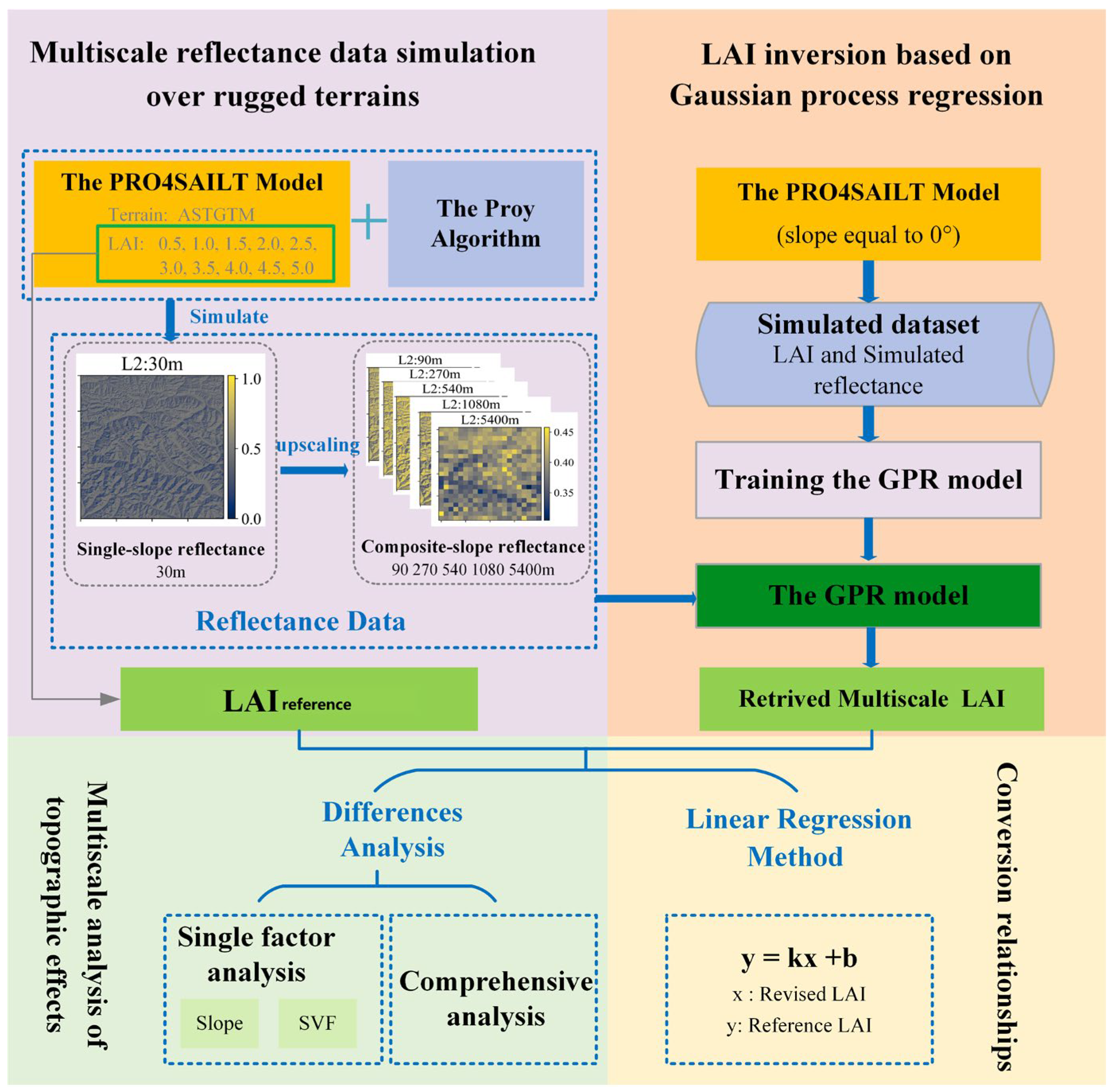
2.1. Multiscale Reflectance Data Simulation over Rugged Terrains

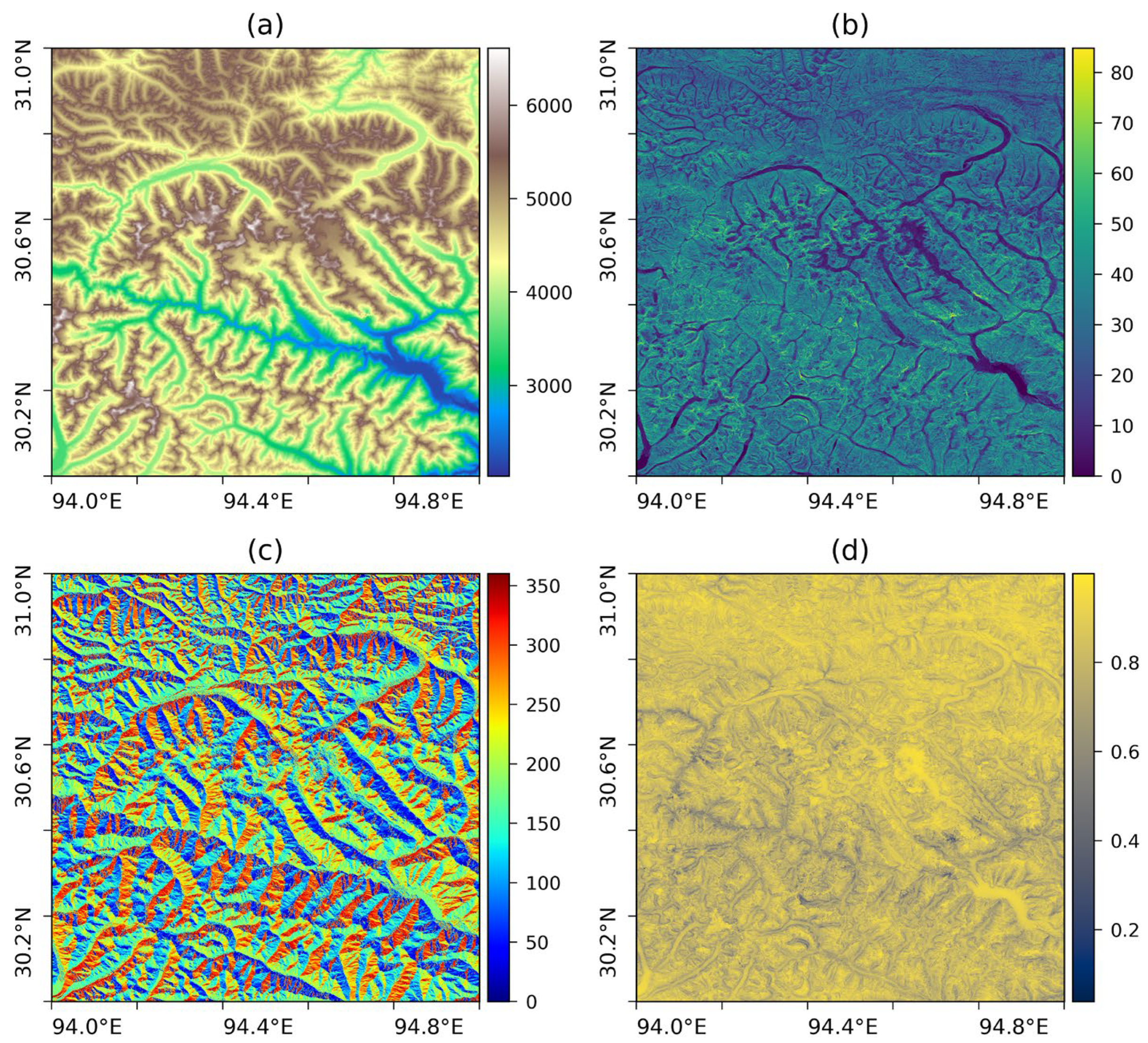
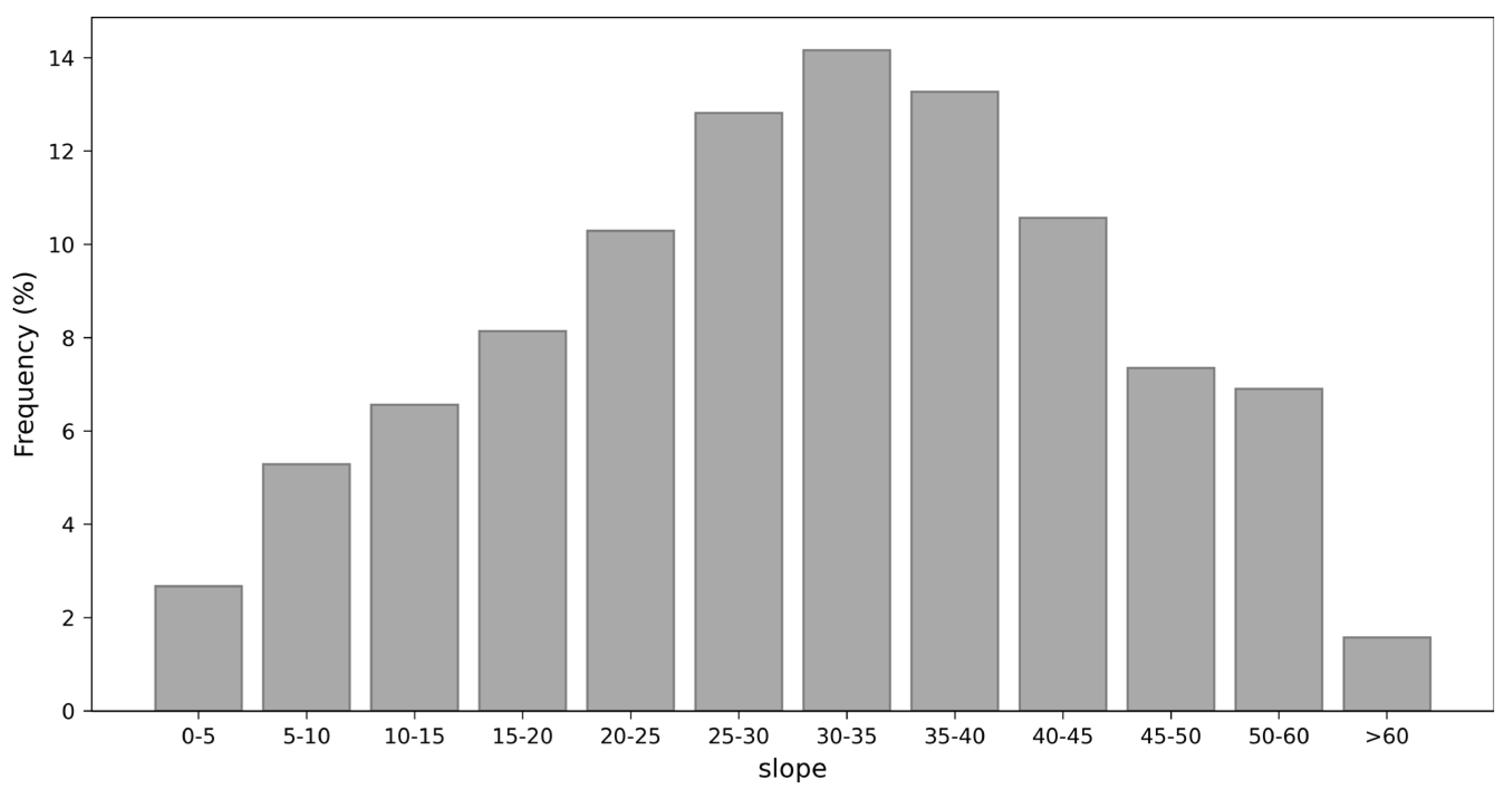
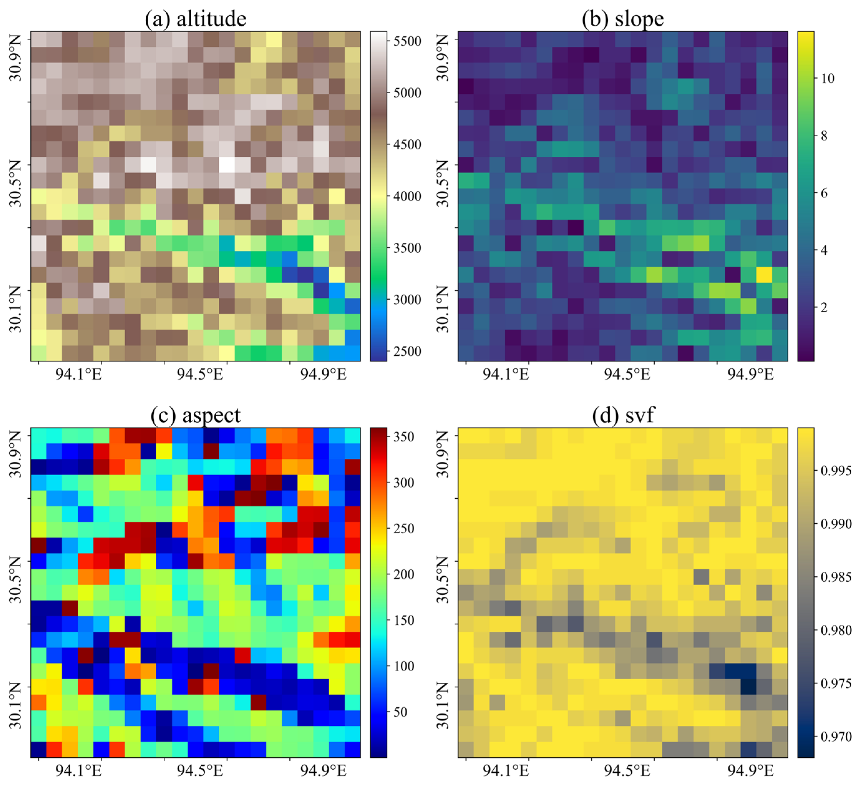
2.1.1. Study Area and Data

In this study, multiscale reflectance data are simulated based on complex terrain conditions in the southern part of the Tibetan Plateau (30°N–31°N, 94°E–95°E). The ASTER Global Digital Elevation Model (ASTGTM) [42] dataset is used to calculate the slope, aspect, and sky visibility factor (SVF) (shown in Figure 2). A frequency distribution histogram of the slope in this area is shown in Figure 3. As shown in the two figures, this area contains terrains under various conditions with slopes ranging from 0 to 80°. Therefore, the simulated reflectance data based on such terrain conditions are more representative and can provide more extensive basic data for a subsequent LAI inversion error analysis. The spatial resolution of the ASTGTM is approximately 30 m. It was resampled to 90, 270, 540, 1080, and 5400 m, respectively. Figure 4 shows the terrain parameters with a resolution of 5400 m. It can be seen that the slope of most pixels is very small (below 6°), and the maximum slope does not exceed 12°. It should be noted that this study only uses the DEM of this area. The actual surface conditions (e.g., the land cover and vegetation growth) are not used. A detailed experimental scheme is described in Section 2.1.2.

2.1.2. Reflectance Data Simulation Based on Topography Models

Topography modeling can be classified into solo-slope modeling and composite-slope modeling according to the size of the target pixels [33]. When the spatial resolutions of the DEM data and remote sensing data are roughly the same, each pixel contains only the unique slope and aspect features; this is called a solo slope. In contrast, when the spatial resolution of the remote sensing data is much lower than that of the DEM data, each pixel in the remote sensing data contains multiple slope and aspect features; this is called a composite slope. Because the spatial resolution of the ASTGTM dataset is approximately 30 m, this paper takes 30 m as the finest spatial resolution (the solo slope) and takes five other spatial resolutions of 90, 270, 540, 1080, and 5400 m as coarse spatial resolutions (the composite slope).

In general, the radiance observed by sensors at the bottom of the atmosphere (BOA) for a solo slope includes not only direct solar radiation and diffuse sky radiation from the target pixel but also the radiance contributed by adjacent slopes; that is, terrain radiation. In this study, a canopy radiative transfer model, PRO4SAILT, is used to simulate direct solar radiation and diffuse sky radiation. And, the Proy algorithm [41] is used to calculate the terrain radiation.

The PRO4SAILT model couples the 4SAILT canopy model [40], the PROSPECT-D leaf model [43], and the Walthall soil model [44]. The 4SAILT model, developed by Shi et al. [40], considers topographic effects on direct solar radiation, the surrounding topography obstruction of hemispherical radiation, and gravitropic influences on the leaf angle distribution (LAD). It is an extension of the 4SAIL model [45]. Three topographic variables (i.e., the slope, aspect, and SVF) are added to the 4SAIL model to consider topographic and gravitropic effects. Like the 4SAIL model, it can simulate canopy radiance in the optical to thermal infrared range. The 4SAILT model is an accurate and efficient model and can be used for forward modeling and parameter inversion from remote sensing data. The PROSPECT-D model is one of the most widely used radiative transfer (RT) models for simulating the optical characteristics of leaves. It simulates the directional hemisphere reflectance and transmittance in the spectral range from 400 nm to 2500 nm. The Walthall model is an empirical soil model that takes into account anisotropic surfaces and requires a soil spectrum to drive the model.

The parameters of the PRO4SAILT model are given in

Table 1. Parameter characteristics of the of the PRO4SAILT model and parameter setting for the experimental scheme.

Model	Parameter	Symbol	Model Parameter Range	Units	Parameter Setting for Reflectance Simulation over Rugged Terrains	Parameter Setting for Simulation of the Training Dataset
Leaf Model PROSPECT-D	Leaf chlorophyll content	Cab	0–100	$\mathsf{\mu }\mathrm{g}/{\mathrm{cm}}^2$	50	5–75	Uniform
	Carotenoids	Car	0–30	$\mathsf{\mu }\mathrm{g}/{\mathrm{cm}}^2$	10	10	-
	Anthocyanin	CAnth	0–20	$\mathsf{\mu }\mathrm{g}/{\mathrm{cm}}^2$	0	0	-
	Brown pigment content	Cbrown	0–1	$\mathsf{\mu }\mathrm{g}/{\mathrm{cm}}^2$	0	0	-
	Leaf water content	Cw	0.0001–0.05	$\mathrm{cm}$	0.010	0.002–0.05	Uniform
	Leaf dry matter content	Cm	0.0001–0.05	$\mathrm{g}/{\mathrm{cm}}^2$	0.0080	0.001–0.03	Uniform
	Leaf structure index	N	1–3.5	None	1.6	1.6	-
Canopy Model 4SAILT	Sun zenith angle	sza	0–90	°	30	30	-
	Sun azimuth angle	saa	0–360	°	130	130	-
	View zenith angle	vza	0–90	°	10	10	-
	View azimuth angle	vaa	0–360	°	40	40	-
	Average leaf inclination angle	ALA	0–90	°	45	30–80	Uniform
	Leaf area index	LAI	0–8	None	0.5, 1, 1.5, 2, 2.5, 3, 3.5, 4, 4.5, 5	0.1–6	Uniform
	Hot spot parameter	hspot	0.001–0.1	None	0	0	-
	Slope	slope	0–90	°	From DEM	0	-
	Aspect	aspect	0–360	°	From DEM	0	-
	Sky view factor	SVF	0–1	None	From DEM	1	-
Soil Model Walthall	Soil parameter 1	s1	0.05–0.4	None	0.4	0.05–0.4	Uniform
	Soil parameter 2	s2	−0.1–0.1	None	0	0	-
	Soil parameter 3	s3	−0.05–0.05	None	0	0	-
	Soil parameter 4	s4	−0.04–0.04	None	0	0	-

. This model has many parameters, but only a portion of them are sensitive to surface reflectance at certain wavelengths. Therefore, a sensitivity analysis of the model is conducted. In this paper, the Extension of the Fourier Amplitude Sensitivity Testing (EFAST) method [46] is used to find the sensitive parameters. It is a variance-based method and has been widely used in the parameter sensitivity analysis of remote sensing physical models [47,48,49]. Figure 5a,b show the first-order sensitivity index (SI) and total-order SI, respectively, of each parameter. We set 0.2 as the reference line for the first-order SI and the total-order SI. If a parameter’s SI value is greater than 0.2, the parameter is considered sensitive. By comprehensively analyzing the first-order and total-order SI, six parameters, namely the leaf area index (LAI), leaf chlorophyll content (C_ab), leaf water content (C_w), leaf dry matter content (C_m), average leaf inclination angle (ALA), and soil model parameter (s1), are determined to be sensitive parameters of the PRO4SAILT model. It is roughly consistent with the sensitive parameters used in other articles for the inversion of LAI values using the PROSAIL model [4,11,12].

To simulate the reflectance data over rugged terrains, the parameter settings of the PRO4SAILT model are given in Table 1. The terrain parameters, such as the slope, aspect, and SVF, are all extracted from the ASTGTM dataset. Moreover, to analyze the influence of terrain on different LAI values, different LAI values ranging from 0.5 to 5 with an interval of 0.5 are considered. The values of the other parameters of the PRO4SAILT model were fixed to certain values, e.g., C_ab is 50 and N is 1.6. These parameters are set with reference to the values of the PROSAILT model parameters in the literature [11,50]. The reflectance values at the center wavelengths of Sentinel-2 in 9 bands (B3, B4, B5, B6, B7, B8, B8A, B11, and B12; 560, 665, 705, 740, 783, 842, 865, 1610 and 2190 nm) under these LAI values are simulated in this study.

The Proy algorithm [41] is used to calculate terrain radiation in this study. Many studies have shown that this algorithm has high accuracy [29,32,51,52,53]. For each pixel in the image, the Proy algorithm calculates the contributions from all surrounding pixels (the effective radius is usually 0.5 to 1.5 km) and the visibility (0 or 1) between any two pixels. The search radius adopted in this study is 1 km, and this process requires iterative processing until a convergence threshold is reached. Therefore, for high-spatial-resolution DEM (e.g., the 30 m DEM used in this study), it is computationally expensive to calculate topographic radiation by using the accurate Proy algorithm [29] because there are hundreds of pixels within the 1 km search radius. Shi et al. [54] used the Proy algorithm to simulate different surface parameters, including surface reflectance and surface radiation, at a series of spatial resolutions (30, 90, 270, 540, 1080, and 5400 m). The results show that two iterations in the simulation of surface reflectance are sufficient. Performing more iterations is not meaningful since doing so requires more time and does not substantially improve accuracy. Therefore, a maximum of two iterations are performed in this study when using the Proy algorithm.

Once the radiance at a fine spatial resolution scale (i.e., the solo slope) is calculated, the corresponding radiance values at coarse spatial resolution scales (i.e., the composite slope) can then be calculated using upscaling procedures [33]. The accuracy of the solo-slope model determines the accuracy of the composite-slope model. As a result, based on the PRO4SAILT model and the Proy algorithm, the surface reflectance at a resolution of 30 m is simulated. Then, the surface reflectance at resolutions of 90, 270, 540, 1080, and 5400 m under the corresponding LAI values are further obtained.

2.2. LAI Inversion Based on Gaussian Process Regression

2.2.1. Gaussian Process Regression

In this study, the Gaussian process regression (GPR) method is used to retrieve LAI values from simulated multiscale reflectance data. GPR is a kernel-based machine learning method [55]. It has good applicability for addressing complex problems such as high dimensionality, small sample size, and nonlinearities, as well as uncertainty prediction capabilities. Moreover, highly importantly, the GPR model can conveniently accommodate different data sources (such as multimodal data, multisensor data, and multitime data) and can be designed to handle different noise sources [9]. The principle of this method is as follows:

From the perspective of function space, a Gaussian process (GP) is defined to describe the distribution of functions, and Bayesian inference is performed directly in the function space. A GP refers to a set in which any finite random variable obeys a Gaussian distribution, and its properties are completely determined by the mean function $\mathrm{m}\left(\mathrm{x}\right)$ and the covariance function $\mathrm{k}(\mathrm{x},{\mathrm{x}}^{\prime })$:

$$\left\{\begin{array}{c}\mathrm{m}\left(\mathrm{x}\right)=\mathrm{E}\left[\mathrm{f}\left(\mathrm{x}\right)\right]\\ \mathrm{k}\left({\mathrm{x},\mathrm{x}}^{\prime }\right)=\mathrm{E}\left[\right(\mathrm{f}\left(\mathrm{x}\right)-\mathrm{m}\left(\mathrm{x}\right)\left)\right(\mathrm{f}\left({\mathrm{x}}^{\prime }\right)-\mathrm{m}\left({\mathrm{x}}^{\prime }\right)\left)\right]\end{array}\right.$$

(1)

where $\mathrm{x},{\mathrm{x}}^{\prime }\in {\mathrm{R}}^{\mathrm{d}}$ represents any random variables; thus, the GP can be defined as $\mathrm{f}\left(\mathrm{x}\right)~\mathrm{GP}\left(\mathrm{m}\right(\mathrm{x}), \mathrm{k}(\mathrm{x},{\mathrm{x}}^{\prime }\left)\right)$. For symbolic simplicity, the data can usually be preprocessed to make their mean function 0.

The noise is taken into account in the target value y, i.e.,

$$\mathrm{y}=\mathrm{f}\left(\mathrm{x}\right)+\mathsf{\epsilon }$$

(2)

where $\mathrm{x}$ represents the input vector; $\mathrm{f}\left(\mathrm{x}\right)$ represents the function value; $\mathrm{y}$ represents the observation value contaminated by noise; and $\mathsf{\epsilon }$ represents the independent Gaussian white noise, which conforms to a Gaussian distribution with a mean value of 0 and a variance of ${\mathsf{\sigma }}^2$ and can be expressed as $\mathsf{\epsilon }~\mathrm{N}(0,{\mathsf{\sigma }}^2)$. Since the noise $\mathsf{\epsilon }$ is white noise independent of $\mathrm{f}\left(\mathrm{x}\right)$, when $\mathrm{f}\left(\mathrm{x}\right)$ obeys a Gaussian distribution, $\mathrm{y}$ also obeys a Gaussian distribution; that is, the prior distribution of the observed value $\mathrm{y}$ is as expressed in (3):

$$\mathrm{y}~\mathrm{N}(0,\mathrm{K}(\mathrm{X},\mathrm{X})+{\mathsf{\sigma }}_{\mathrm{n}}^2{\mathrm{I}}_{\mathrm{n}})$$

(3)

Moreover, the observed value $\mathrm{y}$ and the predicted value $\mathrm{f}\left(\mathrm{x}\right)$ conform to the following joint prior distribution:

$$\left[\begin{array}{c}\mathrm{y}\\ {\mathrm{f}}_{*}\end{array}\right]~\mathrm{N}(0,\left[\begin{array}{cc}\mathrm{K}\left(\mathrm{X},\mathrm{X}\right)+{\mathsf{\sigma }}_{\mathrm{n}}^2{\mathrm{I}}_{\mathrm{n}}& \mathrm{K}(\mathrm{X},{\mathrm{x}}_{*})\\ \mathrm{K}({\mathrm{x}}_{*},\mathrm{X})& \mathrm{k}({\mathrm{x}}_{*},{\mathrm{x}}_{*})\end{array}\right])$$

(4)

where $\mathrm{K}\left(\mathrm{X},\mathrm{X}\right)={\mathrm{K}}_{\mathrm{n}}=\left({\mathrm{k}}_{\mathrm{ij}}\right)$ represents an $\mathrm{n}\times \mathrm{n}$ symmetric positive definite covariance matrix, in which ${\mathrm{k}}_{\mathrm{ij}}=\mathrm{k}({\mathrm{x}}_{\mathrm{i}},{\mathrm{x}}_{\mathrm{j}})$ is used to measure the correlation between ${\mathrm{x}}_{\mathrm{i}}$ and ${\mathrm{x}}_{\mathrm{j}}$; $\mathrm{K}\left(\mathrm{X},{\mathrm{x}}_{*}\right)=\mathrm{K}{({\mathrm{x}}_{*},\mathrm{X})}^{\mathrm{T}}$ represents the n × 1 covariance matrix between test point ${\mathrm{x}}_{*}$ and input X of the training set; $\mathrm{k}({\mathrm{x}}_{*},{\mathrm{x}}_{*})$ represents the covariance of the test point ${\mathrm{x}}_{*}$ with itself; and ${\mathrm{I}}_{\mathrm{n}}$ represents the n-dimensional identity matrix.

The posterior distribution of the predicted value ${\mathrm{f}}_{*}$ can be calculated as

$${\mathrm{f}}_{*}|\mathrm{X},\mathrm{y}, {\mathrm{x}}_{*}~\mathrm{N}(\overline{{\mathrm{f}}_{*}},\mathrm{cov}({\mathrm{f}}_{*}\left)\right)$$

(5)

where

$$\overline{{\mathrm{f}}_{*}}=\mathrm{K}({\mathrm{x}}_{*},\mathrm{X}){[\mathrm{K}\left(\mathrm{X},\mathrm{X}\right)+{\mathsf{\sigma }}_{\mathrm{n}}^2{\mathrm{I}}_{\mathrm{n}}]}^{-1}\mathrm{y}$$

(6)

$$\mathrm{cov}\left({\mathrm{f}}_{*}\right)=\mathrm{k}\left({\mathrm{x}}_{*},{\mathrm{x}}_{*}\right)- \mathrm{K}({\mathrm{x}}_{*},\mathrm{X})\times {[\mathrm{K}\left(\mathrm{X},\mathrm{X}\right)+{\mathsf{\sigma }}_{\mathrm{n}}^2{\mathrm{I}}_{\mathrm{n}}]}^{-1}\mathrm{K}(\mathrm{X},{\mathrm{x}}_{*})$$

(7)

Then, ${\widehat{\mathrm{u}}}_{*}=\overline{{\mathrm{f}}_{*}}$ and ${\widehat{\mathsf{\sigma }}}_{{\mathrm{f}}_{*}}^2=\mathrm{cov}\left({\mathrm{f}}_{*}\right)$ are the mean and variance, respectively, of the predicted value ${\mathrm{f}}_{*}$ corresponding to the test point ${\mathrm{x}}_{*}$.

Different covariance functions, also known as kernel functions, can be selected during training and have a significant impact on the performance of GPR. The commonly used kernel function is the square exponential kernel, which is adopted in this study, namely

$$\mathrm{k}(\mathrm{x},{\mathrm{x}}^{\prime })={\mathsf{\sigma }}_{\mathrm{f}}^2\exp (-\frac{1}{2}{{(\mathrm{x}-{\mathrm{x}}^{\prime })}^{\mathrm{T}}\mathrm{M}}^{-1}(\mathrm{x}-{\mathrm{x}}^{\prime }\left)\right)$$

(8)

where $\mathrm{M}=\mathrm{diag}({\mathrm{l}}^2)$: l represents the variance scale and ${\mathsf{\sigma }}_{\mathrm{f}}^2$ represents the signal variance. Parameter $\mathsf{\theta }=\left\{\mathrm{M},{\mathsf{\sigma }}_{\mathrm{f}}^2,{\mathsf{\sigma }}_{\mathrm{n}}^2\right\}$ represents the hyperparameter, which can generally be obtained by the maximum likelihood method. First, the negative logarithmic likelihood function $\mathrm{L}\left(\mathsf{\theta }\right)=-\log \mathrm{p}\left(\mathrm{y}|\mathrm{X},\mathsf{\theta }\right)$ of the conditional probability of the training samples is established, and the partial derivative of the hyperparameter $\mathsf{\theta }$ is calculated. Then, the Newton method, the conjugate gradient method, and other optimization methods are used to minimize the partial derivative and obtain the optimal solution for the hyperparameter. Here, the negative logarithmic function $\mathrm{L}\left(\mathsf{\theta }\right)$ and the partial derivative form of hyperparameter $\mathsf{\theta }$ are as follows:

$$\mathrm{L}\left(\mathsf{\theta }\right)=\frac{1}{2}{\mathrm{y}}^{\mathrm{T}}{\mathrm{C}}^{-1}\mathrm{y}+\frac{1}{2}\log \left|\mathrm{C}\right|+\frac{\mathrm{n}}{2}\log 2\mathsf{\pi }$$

(9)

$$\frac{\partial \mathrm{L}\left(\mathsf{\theta }\right)}{\partial {\mathsf{\theta }}_{\mathrm{i}}}=\frac{1}{2}\mathrm{tr}\left(\right(\mathsf{\alpha }{\mathsf{\alpha }}^{\mathrm{T}}-{\mathrm{C}}^{-1})\frac{\partial \mathrm{C}}{\partial {\mathsf{\theta }}_{\mathrm{i}}})$$

(10)

where $\mathrm{C}={\mathrm{K}}_{\mathrm{n}}+{\mathsf{\sigma }}_{\mathrm{n}}^2{\mathrm{I}}_{\mathrm{n}}$ and $\mathsf{\alpha }={(\mathrm{K}+{\mathsf{\sigma }}_{\mathrm{n}}^2{\mathrm{I}}_{\mathrm{n}})}^{-1}\mathrm{y}={\mathrm{C}}^{-1}\mathrm{y}$. After obtaining the optimal parameters, the predicted value ${\mathrm{f}}_{*}$ and its variance ${\widehat{\mathsf{\sigma }}}_{{\mathrm{f}}_{*}}^2$ corresponding to the prediction point ${\mathrm{x}}_{\mathrm{*}}$ can be obtained by (6) and (7).

Until now, Gaussian process regression methods have formed their own packages based on different programming languages, such as GPML (http://www.gaussianprocess.org/gpml/code/matlab/doc/, accessed on 11 April 2024) based on the Matlab language and GPy based on Python (https://sheffieldml.github.io/GPy/, accessed on 11 April 2024). This study uses GPyTorch (https://gpytorch.ai/, accessed on 11 April 2024), which is a Gaussian process regression library implemented based on the PyTorch framework that can fully utilize GPUs to speed up the computational efficiency. Unlike most GP packages, GPyTorch does not provide users with a complete GP model. It provides the necessary tools for building a GP model, leaving users with great flexibility and facilitating personalized model customization.

2.2.2. GPR Training and LAI Inversion

For GPR training, a training dataset relating the LAI and surface reflectance simulated by the PRO4SAILT model with a slope equal to 0° is constructed. The six sensitive parameters, namely LAI, C_ab, C_w, C_m, ALA, and s1, are set as uniformly distributed, while the insensitive parameters are set to fixed values. The specific parameter settings are given in Table 1. The Latin hypercube sampling (LHS) method is used to sample these six parameters, which are input into the PRO4SAILT model together with other fixed parameters. The surface reflectance of nine bands (B3, B4, B5, B6, B7, B8, B8A, B11, and B12) corresponding to the Sentinel-2 sensor are simulated. In this study, a training dataset with a sample size of 5000 is constructed, where 75% of the dataset is used to train the GPR model and the other 25% is used to test the GPR model. The input of the GPR model is the simulated surface reflectance values of the 9 bands corresponding to the Sentinel-2 sensor, and the output of the GPR model is the LAI. Figure 6 shows the GPR training accuracy of the LAI inversion model. The results show that the model has a good training performance, with most scatter points occurring near the 1:1 line, an R² value of 0.9611, and an RMSE equal to 0.3558. However, when the LAI values are relatively large, the predicted results are slightly underestimated.

2.2.3. Multiscale Analysis of Topographic Effects

LAI inversion ignoring terrain effects leads to errors in complex terrain regions. This paper analyses the errors from the perspectives of single-factor analysis and comprehensive analysis. The RMSE and MPE are used to quantitatively analyze the error, and the formulas for calculating the RMSE and MPE are as follows:

$$\mathrm{RMSE}=\sqrt{\frac{1}{\mathrm{N}}{\sum }_1^{\mathrm{N}}{({\mathrm{LAI}}_{\mathrm{biased}}-{\mathrm{LAI}}_{\mathrm{reference}})}^2}$$

(11)

$$\mathrm{MPE}=\frac{100\%}{\mathrm{N}}{\sum }_1^{\mathrm{N}}\left|\frac{{\mathrm{LAI}}_{\mathrm{biased}}-{\mathrm{LAI}}_{\mathrm{reference}}}{{\mathrm{LAI}}_{\mathrm{reference}}}\right|$$

(12)

where ${\mathrm{LAI}}_{\mathrm{biased}}$ refers to the LAI values retrieved from the simulated reflectance by the PRO4SAILT model and the Proy algorithm and ${\mathrm{LAI}}_{\mathrm{reference}}$ refers to the given LAI values while simulating the reflectance by the PRO4SAILT model.

Shi et al. found that the slope and SVF well represents the degree of topographic influences and that terrain radiation cannot be ignored for small-SVF areas when using high-spatial-resolution data [54]. So, in the single-factor analysis, the effects of the slope and SVF on LAI inversion over rugged terrains are considered. Line plots are drawn for the errors (the RMSE and MPE) in the LAI inversion results when the LAI_reference values are 1, 2, 3, 4, and 5 at 6 different resolutions (30, 90, 270, 540, 1080, and 5400 m). The variation rules of the two topographic factors, the slope and SVF, for LAI inversion over rugged terrains under different spatial resolutions can be clearly observed. In a comprehensive analysis, heatmaps of the error values (the RMSE and MPE) at different spatial resolutions under different vegetation densities are drawn. Heatmaps can provide a quantitative analysis of the errors caused by ignoring terrain effects in mountain LAI inversion, which is highly important for the development of mountain LAI inversion algorithms.

2.2.4. Conversion Relationships between the Flat LAI and Slope LAI Values

Ignoring topographic effects has a significant impact on LAI inversion over rugged terrains, and the influence will be even greater in high-resolution images. However, most of the current LAI inversion algorithms do not consider the influence of terrain, which is often due to the complexity of radiative transfer models in mountainous areas and difficulties in correcting the reflectance according to the terrain. Researchers generally do not develop specialized inversion methods for mountainous areas. If there is a conversion relationship, the inverted LAI ignoring topographic effects can be directly converted into the corresponding LAI with the consideration of topography. It can not only reduce the complexity of the inversion but also improve the inversion accuracy in the corresponding area. In this study, biased LAI inversions based on simulated surface reflectance data provide an important dataset for constructing the conversion relationship.

This section is devoted to determining the relationships between the flat LAI and slope LAI values. As the LAI inversion error is closely related to the slope values, the larger the slope is, the greater the inversion error. Therefore, we use the linear regression method to find different relationships according to different slope ranges. Taking the slope range of 0°–5° as an example, 2000 pixels in this slope range from the inversion results of 10 LAI values (0.5, 1, 1.5, 2, 2.5, 3, 3.5, 4, 4.5, and 5) are randomly selected to form a dataset, 80% of which is used to determine the relationship and 20% of which is used to verify the accuracy of the relationship.

3. Results

3.1. Analysis of the Simulation Data

Figure 7 shows the simulated multiscale reflectance corresponding to the Sentinel-2 B8 (NIR, 842 nm) band when the LAI is 3.5. The different rows in the figure represent the different spatial resolutions (30, 90, 270, 540, 1080, and 5400 m). The subplots with the title “L0” represent the reflectance simulated without considering the contributions of adjacent slopes. The subplots labeled “L1” and “L2” represent the simulated reflectance when the Proy algorithm is applied for one iteration and two iterations, respectively. With an increase in the number of iterations, the simulation results become more accurate. Therefore, the subplots with the title “L2” have the highest accuracy and are used as the benchmark for further evaluation. The last two columns in Figure 7 show the differences between L2 and L0 and between L2 and L1.

The surface reflectance at 842 nm simulated by the PRO4SAILT model with a slope equal to 0° is 0.4631 when the LAI is 3.5. A comparison of the different rows in Figure 7 reveals that topography has an impact on the reflectance regardless of the spatial resolution. However, with decreasing spatial resolution, the image details are gradually lost, and the reflectance gradually approaches 0.4631. Therefore, the influence of terrain on reflectance simulation decreases with decreasing spatial resolution; conversely, terrain effects cannot be ignored in high-spatial-resolution data. A comparison of the different columns in the same row reveals that the result for L0 is quite different from that for L2. Ignoring the influence of adjacent pixels has a great impact on the reflectance data simulation results. With an increase in the number of iterations, the simulation results become more accurate. Increasing the number of iterations in the Proy algorithm can improve the accuracy of the results; however, this process takes a long time, and the accuracy and calculation efficiency need to be chosen according to the actual situation.

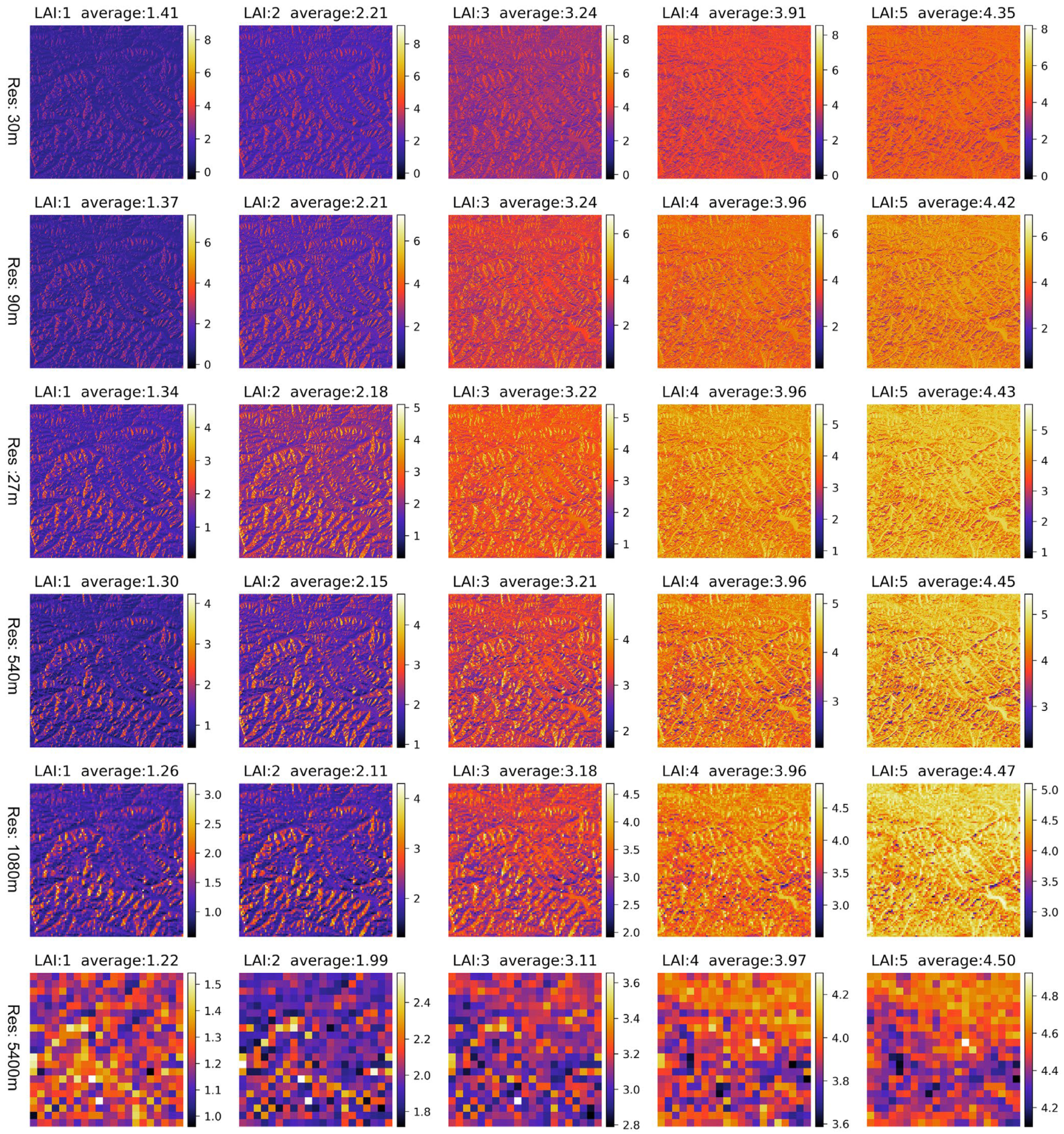
3.2. LAI Values Retrieved Using the Algorithm Ignoring Terrain Effects

The multiscale LAI inversion results based on the two-iteration surface reflectance using the algorithm ignoring terrain effects are shown in Figure 8. Each row includes data at a specific resolution (30, 90, 270, 540, 1080, or 5400 m), and each column represents data at a specific LAI_reference value (1, 2, 3, 4, or 5). The “average” above each subgraph represents the mean of the LAI inversion results for all pixels in the study area. No matter what the spatial resolution is and no matter what the LAI_reference value is, the inversion results obtained using the algorithm ignoring terrain effects will have an impact on the retrieved LAI values over rugged terrains. However, overall, the higher the spatial resolution is, the greater the deviation between the LAI inversion results and LAI_reference values. This phenomenon can not only be seen from the distribution of heat maps, but it is also reflected by the average value of the LAI inversion results. Taking the LAI_reference value of two as an example, when the spatial resolution is 30 m or 90 m, the LAI inversion results are greater than the LAI_reference value in some pixels, and most of these pixels are concentrated over rugged terrains. However, when the spatial resolution gradually decreases from 30 m to 5400 m, that is, from the first row to the last row in Figure 8, the LAI inversion results become closer to the LAI_reference value. At a resolution of 5400 m, the LAI inversion results are almost the same as the LAI_reference value. It can also be intuitively seen from the average value that when the spatial resolution gradually decreases from 30 m to 5400 m, the average value of the LAI inversion results ranges from 2.21 to 1.99, which is getting closer to the LAI_reference value. Taking the LAI_reference value of five as an example, the findings are similar to those for the LAI_reference value of two. Similarly, as the spatial resolution decreases, the results approach the reference value of five. However, the LAI inversion results are generally lower than the LAI_reference values, which is consistent with the GPR training results shown in Figure 6; that is, when the LAI is high, the prediction results are slightly underestimated. Figure 8 demonstrates that terrain has an impact on the retrieved LAI values when the algorithm ignores terrain effects, and this influence is more pronounced for high-spatial-resolution data.

3.3. Multiscale Analysis of Topographic Effects on the Retrieved LAI Values

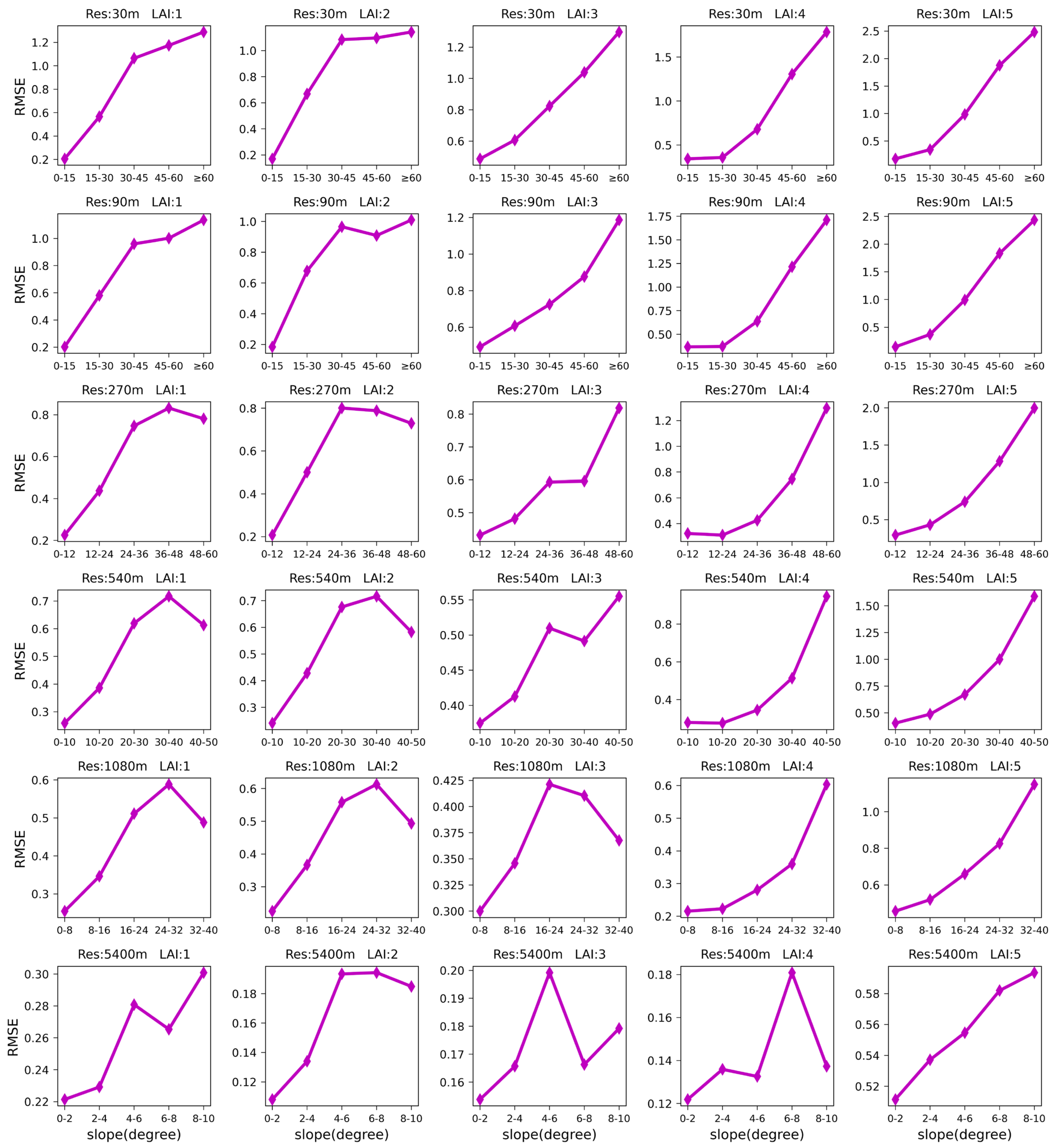
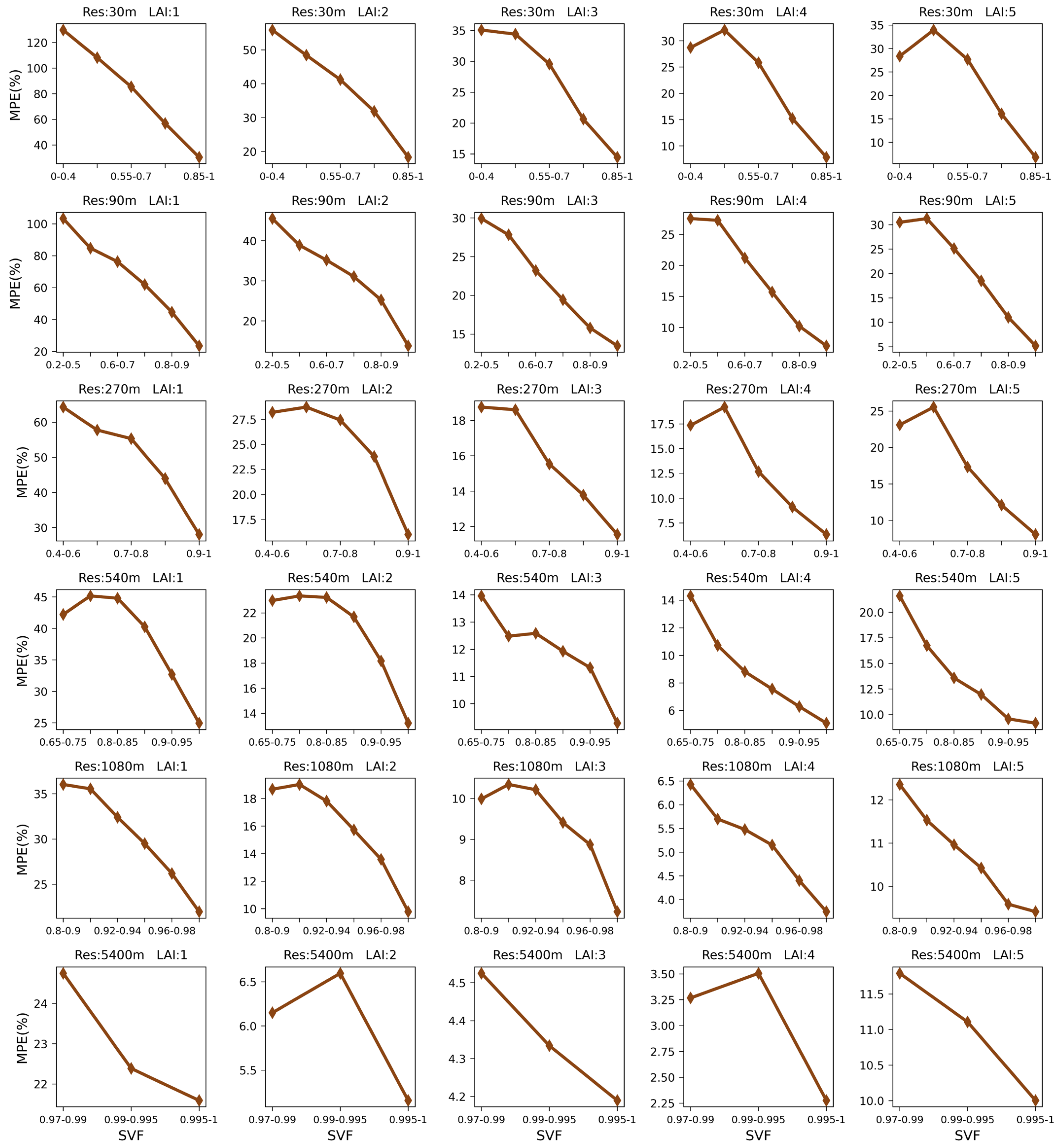
3.3.1. Single Factor Analysis

(1)

Impact analysis of the slope

Figure 9 and Figure 10 show the changes in the RMSE and MPE, respectively, of the multiscale LAI values retrieved using the algorithm ignoring terrain effects. Different rows represent different spatial resolutions (30, 90, 270, 540, 1080, and 5400 m), and different columns represent different LAI_reference values (1, 2, 3, 4, and 5). Figure 9 demonstrates that the RMSE of the retrieved LAI values over rugged terrains generally increases with an increasing slope regardless of the spatial resolution. At resolutions of 1080 m and 5400 m, the RMSE decreases with an increasing slope, which may be due to the small number of pixels with large slopes in coarse-scale images, and the RMSE is not representative. However, the overall trend is that the RMSE increases with an increasing slope, and this trend is observed at different spatial resolutions. Taking the LAI value of five at the resolution of 30 m as an example, when the slope is less than 15°, the RMSE is generally small, about 0.1. When the slope is between 15° and 30°, the RMSE generally does not exceed 0.5. However, when the slope is greater than 45°, the RMSE of the retrieved LAI values is relatively large.

Similarly, Figure 10 shows that the MPE of the LAI values retrieved using the algorithm ignoring terrain effects increases with an increasing slope at various spatial resolutions. For example, when the LAI_reference is five and the spatial resolution is 30 m, the MPE is close to 0; that is, the error is small when the slope is less than 15° and the surface is approximately horizontal. However, when the slope is greater than 15°, the MPE gradually increases. In pixels with slopes of 30°–45°, the MPE is close to 20%. In addition, in pixels with slopes of 45°–60°, the MPE is close to 30%. When the slope is ≥60°, the MPE gets greater. Combining Figure 9 and Figure 10, it is found that the slope plays a great role in LAI inversion over rugged terrains. That is, when inverting the LAI in areas with high slopes, ignoring terrain effects can have a significant impact on the inversion results.

(2)

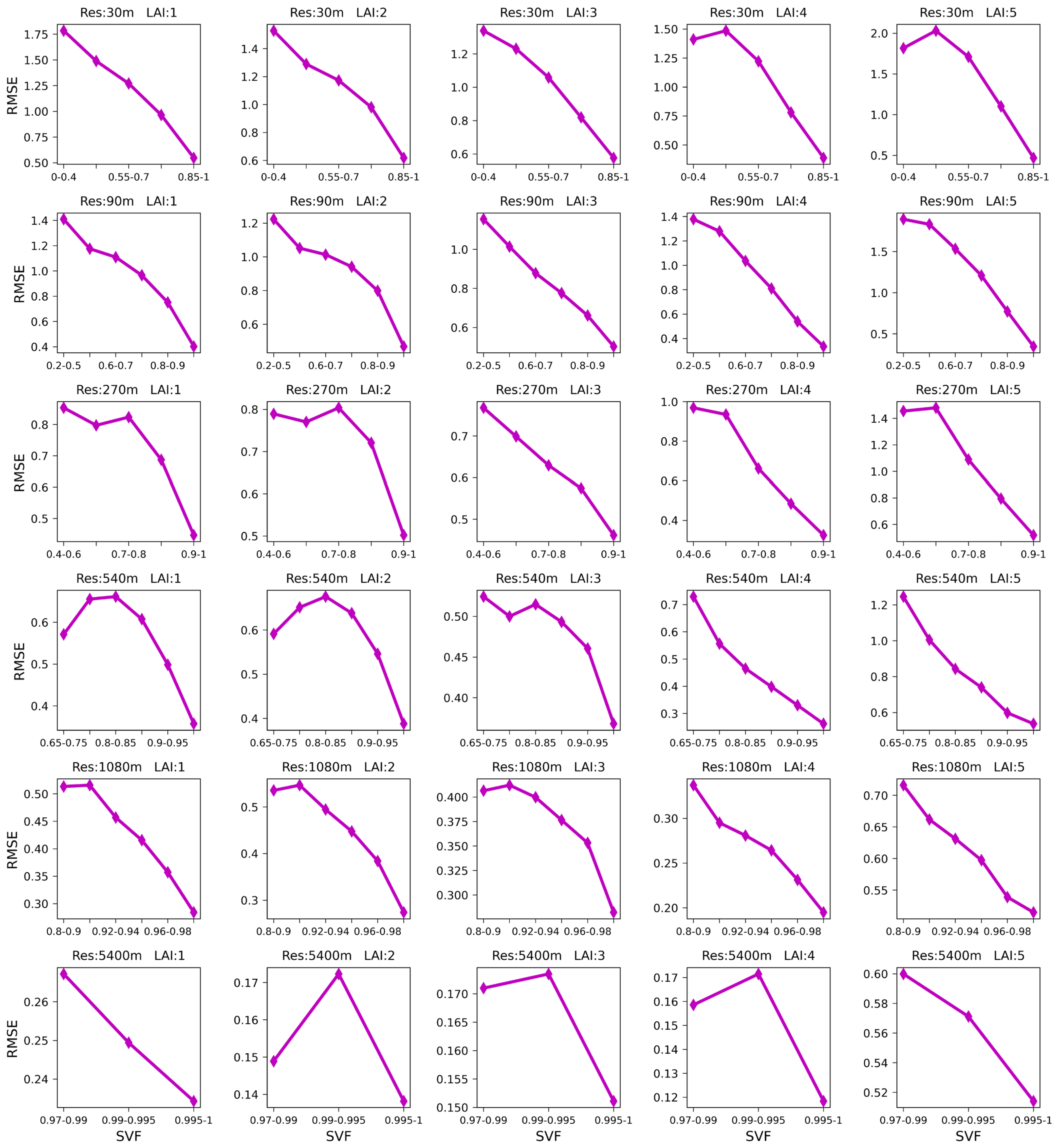
Impact analysis of the SVF

Figure 11 shows the changes in the RMSE of the LAI values retrieved using the algorithm ignoring terrain effects with the SVF. Overall, the larger the SVF is, the smaller the RMSE of the retrieved LAI values. At coarse-scale resolutions, such as 540 and 5400 m, the RMSE increases with an increasing SVF, the reason for which is the number of pixels corresponding to the SVF is low and the RMSE results are not representative.

Figure 12 shows the change in the MPE of the LAI values retrieved using the algorithm ignoring terrain effects with the SVF, which is consistent with the trend of the RMSE variation with the SVF in Figure 11. Regardless of the spatial resolution, overall, the larger the SVF is, the smaller the MPE of the retrieved LAI values. For example, in the subgraph with a LAI_reference value of five and a spatial resolution of 30 m, when the SVF is lower than 0.7, the MPE of the retrieved LAI values is greater than 25%. When the SVF is greater than 0.7, the MPE is relatively low, especially when the SVF is between 0.85 and 1, for which the MPE is less than 10%.

3.3.2. Comprehensive Analysis of Topographic Effects

Figure 13 summarizes the RMSE (a) and MPE (b) of the multiscale LAI values retrieved using the algorithm ignoring terrain effects. The horizontal axis represents different LAI_reference values, and the vertical axis represents different spatial resolutions. Figure 13a shows that the RMSE values of the retrieved LAI values differ under different LAI values. Under the same LAI values, the RMSE of the retrieved LAI values decreases with decreasing spatial resolution. For example, when the LAI_reference value is one, the RMSE of the retrieved LAI values at the scale of 30 m can reach 0.8723. However, with decreasing spatial resolution, the RMSE is 0.6602 at 270 m, 0.4212 at 1080 m, and only 0.2421 at 5400 m. Similarly, when the LAI_reference value is five, the RMSE of the retrieved LAI values gradually increases from 0.5376 to 0.608, 0.6907, 0.7746, 0.8914, and 1.005 as the spatial scale gradually decreases from 5400 to 1080, 540, 270, 90, and 30 m, respectively.

Figure 13b summarizes the MPE of the multiscale LAI values retrieved using the algorithm ignoring terrain effects. The MPE values of the retrieved LAI values differ under different LAI values. Under the same LAI values, the MPE of the retrieved LAI values decreases with decreasing spatial resolution. For example, when the LAI_reference value is one, the MPE of the retrieved LAI values can reach 49.74% at a scale of 30 m. However, with decreasing spatial resolution, the MPE of the retrieved LAI values reached 39.93% at 270 m and 29.59% at 1080 m. At a 5400 m resolution, the RMSE is only 22.19%. When the LAI_reference is five, the MPE of the retrieved LAI increases from 10.46% to 13.72% as the spatial scale increases from 5400 m to 30 m.

3.4. Conversion Relationships between the LAI Values Retrieved Using the Algorithm Ignoring Terrain Effects and the Reference LAI Values

Table 2. Conversion relationships between the LAI values retrieved via the algorithm ignoring terrain effects and the reference LAI values at a resolution of 30 m.

Slope Range	Conversion Relationships (x: Retrieved LAI; y: Reference LAI)
0°–5°	y = 0.9712x − 0.1437
5°–10°	y = 0.9800x − 0.1604
10°–15°	y = 0.9898x − 0.1799
15°–20°	y = 0.9970x − 0.2134
20°–25°	y = 0.9786x − 0.1768
25°–30°	y = 0.9236x − 0.0455

lists the conversion relationships between the LAI values retrieved using the algorithm ignoring terrain effects and the reference LAI values at a resolution of 30 m according to different slope ranges. The relationships are obtained using the linear regression method based on 80% of the samples in the dataset in Section 2.2.2. Figure 14 verifies the accuracy (the RMSE and R²) of these relationships using the remaining 20% of the samples in the dataset in Section 2.2.2, where the horizontal axis represents the true value in this 20% of the sample and the vertical axis represents the converted LAI obtained through the conversion relationship in Table 2. When the slope is between 0° and 5°, the conversion relationship is y = 0.9712x − 0.1437, with high accuracy, as shown in Figure 14a. This is because when the slope is small, the surface is close to being horizontal, and the difference between the retrieved LAI values and the reference LAI values is not significant. However, as the slope increases, the R² value of the conversion relationship decreases and the RMSE increases. When the slope is between 25° and 30°, the R² value of the relationship is only 0.8239, and the RMSE is 0.6025, indicating a relatively low accuracy. When the slope is larger than 30°, the accuracy is even lower, which is not shown in the table. This is because when the slope is greater than 30°, the simple linear relationship is not sufficient to represent the relationship between the retrieved and reference LAI values. However, considering that the slope of most areas in practice does not exceed 30°, the conversion relationships proposed in this study can still provide support for LAI inversion over rugged terrains.

4. Discussion

This paper analyzes the influence of topography on mountain LAI inversion by comparing the LAI values retrieved from multiscale surface reflectance simulated by the PRO4SAILT model and the Proy algorithm over rugged terrains with the corresponding reference LAI data. In this study, all the pixels in the study area are assumed to be identical, except for their topography, during the simulations. This assumption helps identify the influences of topography alone. In addition, because the terrain conditions of the selected study area are complex, with slopes spanning from 0° to 80°, the results can be used to analyze the errors in LAI inversion under various terrain conditions to make the results more comprehensive and objective. Compared with the actual remote sensing reflectance data and the measured LAI, the method proposed in this paper avoids the difficulty of obtaining measured mountain LAI data and actual remote sensing reflectance data. The results demonstrate that the error in the retrieved LAI values increases with an increasing slope. This finding is consistent with that of previous studies [29,32].

However, LAI inversion using simulated reflectance data has several limitations. Firstly, due to the long computation time and large memory space required by the Proy algorithm when simulating the multiscale reflectance data over rugged terrains, we only simulated the reflectance when the PRO4SAILT model parameters were fixed values, e.g., C_ab was chosen to be 50, N was chosen to be 1.6, and so on. Here, in order to analyze the effect of terrain on the inversion of different LAI values, the terrain parameters were taken from the DEM images, and 10 LAI values ranging from 0.5 to 5 at intervals of five were selected. In the future, we will try to simulate the reflectance with other values for these parameters.

Secondly, since actual scenes are much more complicated, the reflectance of each pixel is related to the land cover. During the reflectance simulation process, it is assumed that all the pixels in the study area have the same type of land cover. However, the actual scenario is much more complex, and the heterogeneity among pixels is often large [56]. Additionally, the reflectance simulation does not consider the influence of the atmosphere. The atmosphere between two pixels affects terrain radiation, such as the attenuation of radiation and atmospheric path radiation [57,58]. In summary, the influence of topography is coupled with surface and atmospheric characterizations. Therefore, additional effort is needed when applying this study’s conclusions to practical scenarios.

Thirdly, this study analyzes the effects of slope and the SVF on mountain LAI inversion errors. In general, the larger the slope or the smaller the SVF is, the larger the errors. This approach is highly important for the development of LAI retrieval strategies over rugged terrains. However, this paper discussed only the impact of the slope and the SVF on the LAI retrieval error. Rugged terrain is often complex, and many indicators are available for describing terrain characteristics. Only these two factors are considered here, without considering the heterogeneity of rugged terrains, climate, vegetation type, mountain shadow [59], etc. Therefore, these factors can be included in a mountain LAI error analysis in the future.

In addition, this paper proposes relationships that can be used to directly convert the retrieved LAI ignoring topographic effects into corresponding LAI values with the consideration of topography. The relationships are constructed based on different slope ranges because the LAI inversion error is closely related to the slope, as demonstrated in Figure 9 and Figure 10. In this way, if the slope is less than 30°, the retrieved LAI values using the algorithm ignoring terrain effects can be directly converted into mountain LAI values based on the relationships given in this paper, which greatly reduces the complexity of the inversion of mountain LAI values. However, these relationships also have certain limitations. The relationships are based on the linear regression method. When the slope is large, a simple linear relation may not be able to summarize all the relevant situations, resulting in a decrease in the inversion accuracy. Furthermore, these relationships have been validated only based on simulated data. Therefore, it is necessary to construct a universal and simple LAI inversion strategy over rugged terrains. These topics need to be explored in depth in the future.

5. Conclusions

This study explored the topographic effects on LAI retrieval from surface reflectance data at various spatial scales (30, 90, 270, 540, 1080, and 5400 m) over rugged terrains. The PRO4SAILT model and the Proy algorithm were used to simulate surface reflectance at the 30 m scale for different LAI values (0.5, 1.0, 1.5, 2.0, 2.5, 3.0, 3.5, 4.0, 4.5, and 5.0). Reflectance data at spatial scales of 90 m, 270 m, 540 m, 1080 m, and 5400 m were obtained by an upscaling method. To improve the universality of the results, complex terrain conditions were used in the simulation. Based on the simulation data, the topographic effects of multiscale LAI inversion were quantitatively analyzed. The results demonstrated that the higher the spatial resolution is, the greater the error in the retrieved LAI values. Regardless of the spatial resolution, the error in the retrieved LAI values increases with an increasing slope. The larger the sky visibility factor is, the smaller the error in the retrieved LAI values. This study also constructed linear regression relationships to convert the retrieved LAI values using an algorithm that ignores terrain effects to mountain LAI values according to different slope ranges.

These conclusions provide a reference for those interested in estimating LAI values over mountain areas from remote sensing data at various spatial scales. Future studies will focus on constructing LAI inversion algorithms for mountainous areas based on radiation transfer models.

References

1. Jin, H.; Li, A.; Wang, J.; Bo, Y. Improvement of Spatially and Temporally Continuous Crop Leaf Area Index by Integration of CERES-Maize Model and MODIS Data. Eur. J. Agron. 2016, 78, 1–12. [Google Scholar] [CrossRef]
2. Martin, C.; Jessica, M.; Eric, V.; Christopher, J. A 30+ Year AVHRR LAI and FAPAR Climate Data Record: Algorithm Description and Validation. Remote Sens. 2016, 8, 263. [Google Scholar] [CrossRef]
3. Chen, J.M.; Black, T.A. Defining Leaf Area Index for Non-flat Leaves. Agric. For. Meteorol. 1992, 15, 421–429. [Google Scholar] [CrossRef]
4. Baret, F.; Hagolle, O.; Geiger, B.; Bicheron, P.; Miras, B.; Huc, M.; Berthelot, B.; Niño, F.; Weiss, M.; Samain, O.; et al. LAI, fAPAR and fCover CYCLOPES Global Products Derived from VEGETATION Part 1: Principles of the Algorithm. Remote Sens. Environ. 2009, 110, 275–286. [Google Scholar] [CrossRef]
5. Xiao, Z.; Liang, S.; Wang, J.; Chen, P.; Yin, X.; Zhang, L.; Song, J. Use of General Regression Neural Networks for Generating the GLASS Leaf Area Index Product from Time-Series MODIS Surface Reflectance. IEEE Trans. Geosci. Remote Sens. 2014, 52, 209–223. [Google Scholar] [CrossRef]
6. Baret, F.; Weiss, M.; Lacaze, R.; Camacho, F.; Makhmara, H.; Pacholcyzk, P.; Smets, B. GEOV1: LAI and FAPAR Essential Climate Variables and FCOVER Global Time Series Capitalizing over Existing Products. Part1: Principles of Development and Production. Remote Sens. Environ. 2013, 137, 299–309. [Google Scholar] [CrossRef]
7. Zhu, Z.; Bi, J.; Pan, Y.; Ganguly, S.; Anav, A.; Xu, L.; Samanta, A.; Piao, S.; Nemani, R.R.; Myneni, R.B. Global Data Sets of Vegetation Leaf Area Index (LAI)3g and Fraction of Photosynthetically Active Radiation (FPAR)3g Derived from Global Inventory Modeling and Mapping Studies (GIMMS) Normalized Difference Vegetation Index (NDVI3g) for the Period 1981 to 2011. Remote Sens. 2013, 5, 927–948. [Google Scholar] [CrossRef]
8. Atzberger, C. Object-Based Retrieval of Biophysical Canopy Variables Using Artificial Neural Nets and Radiative Transfer Models. Remote Sens. Environ. 2004, 93, 53–67. [Google Scholar] [CrossRef]
9. Camps-Valls, G.; Verrelst, J.; Munoz-Mari, J.; Laparra, V.; Mateo-Jimenez, F.; Gomez-Dans, J. A Survey on Gaussian Processes for Earth-Observation Data Analysis: A Comprehensive Investigation. IEEE Geosci. Remote Sens. Mag. 2016, 4, 58–78. [Google Scholar] [CrossRef]
10. Gewali, U.B.; Monteiro, S.T.; Saber, E. Gaussian Processes for Vegetation Parameter Estimation from Hyperspectral Data with Limited Ground Truth. Remote Sens. 2019, 11, 1614. [Google Scholar] [CrossRef]
11. Estévez, J.; Vicent, J.; Rivera-Caicedo, J.P.; Morcillo-Pallarés, P.; Vuolo, F.; Sabater, N.; Camps-Valls, G.; Moreno, J.; Verrelst, J. Gaussian Processes Retrieval of LAI from Sentinel-2 Top-of-Atmosphere Radiance Data. ISPRS J. Photogramm. Remote Sens. 2020, 167, 289–304. [Google Scholar] [CrossRef] [PubMed]
12. Adeluyi, O.; Harris, A.; Verrelst, J.; Foster, T.; Clay, G.D. Estimating the Phenological Dynamics of Irrigated Rice Leaf Area Index Using the Combination of PROSAIL and Gaussian Process Regression. Int. J. Appl. Earth Obs. Geoinf. 2021, 102, 102454. [Google Scholar] [CrossRef] [PubMed]
13. Myneni, R.B.; Hoffman, S.; Knyazikhin, Y.; Privette, J.L.; Glassy, J.; Tian, Y.; Wang, Y.; Song, X.; Zhang, Y.; Smith, G.R.; et al. Global Products of Vegetation Leaf Area and Fraction Absorbed PAR from Year One of MODIS Data. Remote Sens. Environ. 2002, 83, 214–231. [Google Scholar] [CrossRef]
14. Allan, R.P.; Soden, B.J. Atmospheric Warming and the Amplification of Precipitation Extremes. Science 2008, 321, 1481–1484. [Google Scholar] [CrossRef] [PubMed]
15. Jin, M.; Dickinson, R.E. New Observational Evidence for Global Warming from Satellite. Geophys. Res. Lett. 2002, 29, 39-1–39-4. [Google Scholar] [CrossRef]
16. Vinnikov, K.Y.; Grody, N.C. Global Warming Trend of Mean Tropospheric Temperature Observed by Satellites. Science 2003, 302, 269–272. [Google Scholar] [CrossRef]
17. Potter, C.S. Terrestrial Biomass and the Effects of Deforestation on the Global Carbon Cycle. BioScience 1999, 49, 769–778. [Google Scholar] [CrossRef]
18. Jung, M. Global Patterns of Land-Atmosphere Fluxes of Carbon Dioxide, Latent Heat, and Sensible Heat Derived from Eddy Covariance, Satellite, and Meteorological Observations. J. Geophys. Res. Biogeosci. 2011, 116, G00J07. [Google Scholar] [CrossRef]
19. Julien, Y.; Sobrino, J.A. Global Land Surface Phenology Trends from GIMMS Database. Int. J. Remote Sens. 2009, 30, 3495–3513. [Google Scholar] [CrossRef]
20. Zhang, X.; Friedl, M.A.; Schaaf, C.B.; Strahler, A.H.; Hodges, J.C.; Gao, F.; Reed, B.C.; Huete, A. Monitoring Vegetation Phenology Using MODIS. Remote Sens. Environ. 2003, 84, 471–475. [Google Scholar] [CrossRef]
21. Townshend, J.; Justice, C.; Li, W.; Gurney, C.; Mcmanus, J. Global Land Cover Classification by Remote Sensing: Present Capabilities and Future Possibilities. Remote Sens. Environ. 1991, 35, 243–255. [Google Scholar] [CrossRef]
22. Jin, H.; Li, A.; Bian, J.; Nan, X.; Zhao, W.; Zhang, Z.; Yin, G. Intercomparison and Validation of MODIS and GLASS Leaf Area Index (LAI) Products over Mountain Areas: A Case Study in Southwestern China. Int. J. Appl. Earth Obs. Geoinf. 2017, 55, 52–67. [Google Scholar] [CrossRef]
23. Duveiller, G.; Defourny, P. A Conceptual Framework to Define the Spatial Resolution Requirements for Agricultural Monitoring Using Remote Sensing. Remote Sens. Environ. 2010, 114, 2637–2650. [Google Scholar] [CrossRef]
24. Mulla, D.J. Twenty Five Years of Remote Sensing in Precision Agriculture: Key Advances and Remaining Knowledge Gaps. Biosyst. Eng. 2013, 114, 358–371. [Google Scholar] [CrossRef]
25. Seelan, S.K.; Laguette, S.; Casady, G.M.; Seielstad, G.A. Remote Sensing Applications for Precision Agriculture: A Learning Community Approach. Remote Sens. Environ. 2003, 88, 157–169. [Google Scholar] [CrossRef]
26. Asner, G.P.; Powell, G.V.N.; Mascaro, J.; Knapp, D.E.; Clark, J.K.; Jacobson, J.; Kennedy-Bowdoin, T.; Balaji, A.; Paez-Acosta, G.; Victoria, E.; et al. High-Resolution Forest Carbon Stocks and Emissions in the Amazon. Proc. Natl. Acad. Sci. USA 2010, 107, 16738–16742. [Google Scholar] [CrossRef] [PubMed]
27. Sobrino, J.A.; Oltra-Carrió, R.; Sòria, G.; Bianchi, R.; Paganini, M. Impact of Spatial Resolution and Satellite Overpass Time on Evaluation of the Surface Urban Heat Island Effects. Remote Sens. Environ. 2012, 117, 50–56. [Google Scholar] [CrossRef]
28. Welch, R. Spatial Resolution Requirements for Urban Studies. Int. J. Remote Sens. 1982, 3, 139–146. [Google Scholar] [CrossRef]
29. Mousivand, A.; Verhoef, W.; Menenti, M.; Gorte, B. Modeling Top of Atmosphere Radiance over Heterogeneous Non-Lambertian Rugged Terrain. Remote Sens. 2015, 7, 8019–8044. [Google Scholar] [CrossRef]
30. Yin, G.; Li, A.; Zhao, W.; Jin, H.; Bian, J.; Wu, S. Modeling Canopy Reflectance over Sloping Terrain Based on Path Length Correction. IEEE Trans. Geosci. Remote Sens. 2017, 55, 4597–4609. [Google Scholar] [CrossRef]
31. Gonsamo, A.; Chen, J.M. Improved LAI Algorithm Implementation to MODIS Data by Incorporating Background, Topography, and Foliage Clumping Information. IEEE Trans. Geosci. Remote Sens. 2014, 52, 1076–1088. [Google Scholar] [CrossRef]
32. Yu, W.; Li, J.; Liu, Q.; Yin, G.; Zeng, Y.; Lin, S.; Zhao, J. A Simulation-Based Analysis of Topographic Effects on LAI Inversion over Sloped Terrain. IEEE J. Sel. Top. Appl. Earth Obs. Remote Sens. 2020, 13, 794–806. [Google Scholar] [CrossRef]
33. Wen, J.; Liu, Q.; Xiao, Q.; Liu, Q.; You, D.; Hao, D.; Wu, S.; Lin, X. Characterizing Land Surface Anisotropic Reflectance over Rugged Terrain: A Review of Concepts and Recent Developments. Remote Sens. 2018, 10, 370. [Google Scholar] [CrossRef]
34. Wang, K.; Zhou, X.; Liu, J.; Sparrow, M. Estimating Surface Solar Radiation over Complex Terrain Using Moderate-resolution Satellite Sensor Data. Int. J. Remote Sens. 2005, 26, 47–58. [Google Scholar] [CrossRef]
35. Wen, J.; Liu, Q.; Liu, Q.; Xiao, Q.; Li, X. Scale Effect and Scale Correction of Land-Surface Albedo in Rugged Terrain. Int. J. Remote Sens. 2009, 30, 5397–5420. [Google Scholar] [CrossRef]
36. Burgess, D.W.; Lewis, P.; Muller, J.-P.A.L. Topographic Effects in AVHRR NDVI Data. Remote Sens. Environ. 1995, 54, 223–232. [Google Scholar] [CrossRef]
37. Gonsamo, A.; Pellikka, P. The Computation of Foliage Clumping Index Using Hemispherical Photography. Agric. For. Meteorol. 2009, 149, 1781–1787. [Google Scholar] [CrossRef]
38. María Luisa, E.; Frédéric, B.; Marie, W. Slope Correction for LAI Estimation from Gap Fraction Measurements. Agric. For. Meteorol. 2008, 148, 1553–1562. [Google Scholar] [CrossRef]
39. Yan, G.; Hu, R.; Luo, J.; Weiss, M.; Jiang, H.; Mu, X.; Xie, D.; Zhang, W. Review of Indirect Optical Measurements of Leaf Area Index: Recent Advances, Challenges, and Perspectives. Agric. For. Meteorol. 2019, 265, 390–411. [Google Scholar] [CrossRef]
40. Shi, H.; Xiao, Z. The 4SAILT Model: An Improved 4SAIL Canopy Radiative Transfer Model for Sloping Terrain. IEEE Trans. Geosci. Remote Sens. 2021, 59, 5515–5525. [Google Scholar] [CrossRef]
41. Proy, C.; Tanré, D.; Deschamps, P.Y. Evaluation of Topographic Effects in Remotely Sensed Data. Remote Sens. Environ. 1989, 30, 21–32. [Google Scholar] [CrossRef]
42. Fujisada, H.; Urai, M.; Iwasaki, A. Technical Methodology for ASTER Global DEM. IEEE Trans. Geosci. Remote Sens. 2012, 50, 3725–3736. [Google Scholar] [CrossRef]
43. Feret, J.-B.; François, C.; Asner, G.P.; Gitelson, A.A.; Martin, R.E.; Bidel, L.P.R.; Ustin, S.L.; le Maire, G.; Jacquemoud, S. PROSPECT-4 and 5: Advances in the Leaf Optical Properties Model Separating Photosynthetic Pigments. Remote Sens. Environ. 2008, 112, 3030–3043. [Google Scholar] [CrossRef]
44. Walthall, C.L.; Norman, J.M.; Welles, J.M.; Campbell, G.; Blad, B.L. Simple Equation to Approximate the Bidirectional Reflectance from Vegetative Canopies and Bare Soil Surfaces. Appl. Opt. 1985, 24, 383. [Google Scholar] [CrossRef] [PubMed]
45. Verhoef, W.; Jia, L.; Xiao, Q.; Su, Z. Unified Optical-Thermal Four-Stream Radiative Transfer Theory for Homogeneous Vegetation Canopies. IEEE Trans. Geosci. Remote Sens. 2007, 45, 1808–1822. [Google Scholar] [CrossRef]
46. Saltelli, A.; Annoni, P.; Azzini, I.; Campolongo, F.; Ratto, M.; Tarantola, S. Variance Based Sensitivity Analysis of Model Output. Design and Estimator for the Total Sensitivity Index. Comput. Phys. Commun. 2010, 181, 259–270. [Google Scholar] [CrossRef]
47. Mousivand, A.; Menenti, M.; Gorte, B.; Verhoef, W. Global Sensitivity Analysis of the Spectral Radiance of a Soil–Vegetation System. Remote Sens. Environ. 2014, 145, 131–144. [Google Scholar] [CrossRef]
48. Verrelst, J.; Rivera, J.P.; van der Tol, C.; Magnani, F.; Mohammed, G.; Moreno, J. Global Sensitivity Analysis of the SCOPE Model: What Drives Simulated Canopy-Leaving Sun-Induced Fluorescence? Remote Sens. Environ. 2015, 166, 8–21. [Google Scholar] [CrossRef]
49. Prikaziuk, E.; van der Tol, C. Global Sensitivity Analysis of the SCOPE Model in Sentinel-3 Bands: Thermal Domain Focus. Remote Sens. 2019, 11, 2424. [Google Scholar] [CrossRef]
50. Berger, K.; Atzberger, C.; Danner, M.; Wocher, M.; Mauser, W.; Hank, T. Model-Based Optimization of Spectral Sampling for the Retrieval of Crop Variables with the PROSAIL Model. Remote Sens. 2018, 10, 2063. [Google Scholar] [CrossRef]
51. Yan, G.; Wang, T.; Jiao, Z.; Mu, X.; Zhao, J.; Chen, L. Topographic Radiation Modeling and Spatial Scaling of Clear-Sky Land Surface Longwave Radiation over Rugged Terrain. Remote Sens. Environ. 2016, 172, 15–27. [Google Scholar] [CrossRef]
52. Yan, G.; Jiao, Z.-H.; Wang, T.; Mu, X. Modeling Surface Longwave Radiation over High-Relief Terrain. Remote Sens. Environ. 2020, 237, 111556. [Google Scholar] [CrossRef]
53. Jiao, Z.-H.; Yan, G.; Wang, T.; Mu, X.; Zhao, J. Modeling of Land Surface Thermal Anisotropy Based on Directional and Equivalent Brightness Temperatures over Complex Terrain. IEEE J. Sel. Top. Appl. Earth Obs. Remote Sens. 2019, 12, 410–423. [Google Scholar] [CrossRef]
54. Shi, H.; Xiao, Z. Exploring Topographic Effects on Surface Parameters over Rugged Terrains at Various Spatial Scales. IEEE Trans. Geosci. Remote Sens. 2022, 60, 4404616. [Google Scholar] [CrossRef]
55. Rasmussen, C.E.; Williams, C.K.I. Gaussian Processes for Machine Learning; Adaptive computation and machine learning; MIT Press: Cambridge, MA, USA, 2006; ISBN 978-0-262-18253-9. [Google Scholar]
56. Riley, S.J.; DeGloria, S.D.; Elliot, R. Index That Quantifies Topographic Heterogeneity. Intermt. J. Sci. 1999, 5, 23–27. [Google Scholar]
57. Liang, S.; Strahler, A.H. An Analytic Radiative Transfer Model for a Coupled Atmosphere and Leaf Canopy. J. Geophys. Res. Atmos. 1995, 100, 5085–5094. [Google Scholar] [CrossRef]
58. Shi, H.; Xiao, Z.; Wen, J.; Wu, S. An Optical-Thermal Surface-Atmosphere Radiative Transfer Model Coupling Framework with Topographic Effects. IEEE Trans. Geosci. Remote Sens. 2021, 60, 4400312. [Google Scholar] [CrossRef]
59. Soenen, S.A.; Peddle, D.R.; Coburn, C.A. SCS+C: A Modified Sun-Canopy-Sensor Topographic Correction in Forested Terrain. IEEE Trans. Geosci. Remote Sens. 2005, 43, 2148–2159. [Google Scholar] [CrossRef]
Figure 1. Flowchart of the exploration of topographic effects on LAI inversion over rugged terrains.
Remotesensing 16 01404 g001
Figure 2. Terrain parameters in the southern part of the Tibetan Plateau (30°N–31°N, 94°E–95°E) with the resolution of 30 m. (a) Elevation in meters. (b) Slope in degrees. (c) Aspect in degrees. (d) SVF.
Remotesensing 16 01404 g002
Figure 3. Histogram of the frequency distribution of the slope in the southern part of the Tibetan Plateau (30°N–31°N, 94°E–95°E).
Remotesensing 16 01404 g003
Figure 4. Terrain parameters in the southern part of the Tibetan Plateau (30°N–31°N, 94°E–95°E) with the resolution of 5400 m.
Remotesensing 16 01404 g004
Figure 5. Sensitivity analysis of the PRO4SAILT model. (a) First-order SI. (b) Total-order SI.
Remotesensing 16 01404 g005
Figure 6. GPR training accuracy of the LAI inversion model.
Remotesensing 16 01404 g006
Figure 7. Multiscale surface reflectance simulation data (LAI = 3.5, 842 nm).
Remotesensing 16 01404 g007
Figure 8. Retrieved multiscale LAI values obtained using the algorithm ignoring terrain effects (LAIreference = 1, 2, 3, 4, and 5).
Remotesensing 16 01404 g008
Figure 9. Changes in the RMSE of the retrieved LAI values obtained using the algorithm ignoring terrain effects with slope.
Remotesensing 16 01404 g009
Figure 10. Changes in the MPE of the retrieved LAI values obtained using the algorithm ignoring terrain effects with slope.
Remotesensing 16 01404 g010
Figure 11. Changes in the RMSE of the LAI values retrieved using the algorithm ignoring terrain effects with the SVF.
Remotesensing 16 01404 g011
Figure 12. Changes in the MPE of the LAI values retrieved using the algorithm ignoring terrain effects with the SVF.
Remotesensing 16 01404 g012
Figure 13. The (a) RMSE and (b) MPE of the LAI values retrieved using the algorithm ignoring terrain effects.
Remotesensing 16 01404 g013
Figure 14. Accuracy (RMSE and R2) of the conversion relationships for different slope ranges (X represents the true LAI and Y represents the LAI obtained through the conversion relationship). The dotted line is the 1:1 line. (a) 0°–5°, (b) 5°–10°, (c) 10°–15°, (d) 15°–20°, (e) 20°–25°, and (f) 25°–30°.
Remotesensing 16 01404 g014