Vertical Features of Volatile Organic Compounds and Their Potential Photochemical Reactivities in Boundary Layer Revealed by In-Situ Observations and Satellite Retrieval

Abstract

Based on in-situ vertical observations of volatile organic compounds (VOCs) in the lower troposphere (0–1.0 km) in Nanjing, China, during the summer and autumn, we analyzed the VOCs vertical profiles, diurnal variation, and their impact factors in meteorology and photochemistry. The results showed that almost all the concentrations of VOC species decreased with height, similar to the profiles of primary air pollutants, as expected. However, we found the ratios of inactive species (e.g., acetylene) and secondary VOCs (e.g., ketones and aldehydes) in total VOCs (TVOCs) increased with height. Combined with satellite-retrieved data, we found the average HCHO tropospheric column concentrations were 2.0 times higher in the summer than in the autumn. While the average of tropospheric NO₂ column concentrations was 3.0 times lower in the summer than in the autumn, the seasonal differences in the ratio of oxygenated VOCs (OVOCs) to NO₂ (e.g., HCHO/NO₂) shown in TROPOMI satellite-retrieved data were consistent with in-situ observations (e.g., acetone/NO₂). On average, during autumn daytime, the mixing layer (ML), stable boundary layer (SBL), and residual layer (RL) had OH loss rates (LOH) of 6.9, 6.3, and 5.5 s⁻¹, respectively. The LOH of alkenes was the largest in the ML, while the LOH of aromatics was the largest in the SBL and RL. At autumn night, the NO₃ loss rates (LNO₃) in the SBL and RL were 2.0 × 10⁻² and 1.6 × 10⁻² s⁻¹, respectively, and the LNO₃ of aromatics was the largest in the SBL and RL. In the daytime of summer, the LOH of VOCs was ~40% lower than that in autumn in all layers, while there was no significant difference in LNO₃ at night between the two seasons. This study provides data support and a theoretical basis for VOC composite pollution control in the Nanjing region.

1. Introduction

Volatile organic compounds (VOCs) generate gaseous pollutants, such as ozone (O₃) and secondary organic aerosols (SOA), through photochemical reactions under solar radiation. As precursors of O₃ and SOA, VOCs play two-tier roles in ozone and PM_2.5 pollution [1]. Since vigorously implementing the “Air Pollution Prevention and Control Action Plan”, China has achieved remarkable success in reducing emissions of particulate matter. However, issues related to VOCs and photochemical pollution remain severe [2]. In urban areas, controlling VOC emissions is an effective way to mitigate ozone pollution. Therefore, an in-depth understanding of VOCs’ photochemical reaction characteristics is imperative for O₃ pollution control.

Numerous scholars have conducted domestic and international research on the concentration levels, spatial and temporal distribution characteristics, chemical reactivity, and source apportionment of VOCs. The attention to VOCs can be traced back to the Los Angeles photochemical smog era [3,4,5,6,7]. Haagen et al. [3] pointed out that VOCs, along with NOx, underwent a series of photochemical reactions in the atmosphere to form the irritating gas O₃ in photochemical smog. Gee et al. [8] compared the concentrations of VOCs in some cities in Europe, America, and Asia and found that the VOC concentrations in Asia were the highest. The VOC concentrations in Vienna, Europe [9], Sydney, Oceania [10], Atlanta, North America [11], and Osaka, Asia [12] were 283.2, 279.9, 332.3, and 501.2 mg/m³, respectively. Domestically, research on VOCs can be traced back to the photochemical smog era in Lanzhou. In recent years, research locations have been mainly concentrated in economically developed regions such as Beijing-Tianjin-Hebei, the Yangtze River Delta, and the Pearl River Delta [13,14,15].

There are many species of VOCs, and the chemical properties of each species vary greatly, leading to differing contributions to O₃ generation when participating in photochemical reactions [16]. The contribution to photochemical O₃ production does not directly correlate with VOC concentrations [17] but is determined by photochemical reactivity. Even high concentrations of low-reactivity species may not significantly impact O₃ production, while trace concentration species with high reactivity contribute significantly to photochemical O₃ generation. In most Chinese areas, alkanes comprise the highest proportion of VOCs [18,19,20], but highly reactive alkenes drive most O₃ production as the main chemical contributors [21,22]. For example, Hui et al. [21] investigated the photochemical reactivity characteristics of VOCs in Wuhan and found that alkenes only accounted for 10.9% of the total VOC concentration but contributed 47.0% to the OH radical loss rate (LOH) and 49.5% to the ozone formation potential (OFP). The seasonal variations of VOCs and OFP are mostly ascribed to the seasonal differences in atmospheric diffusion and photochemical reactivity of VOCs. Lin et al. [22] found that in the northern Nanjing suburbs, the contribution of alkenes to OFP was the largest in the autumn and smallest in the summer, which was consistent with the seasonal changes in their concentration. Additionally, in economically developed urban areas, although anthropogenic VOCs (AVOCs) emissions were relatively large, the contribution of biogenic VOCs (BVOCs) to O₃ production cannot be ignored [23]. Liu et al. [24] found that the contribution of BVOCs to O₃ generation in the Yangtze River Delta region in summer was 4.2 μg/m³.

At present, the detection of vertical profiles of boundary layer (BL) VOCs is still in the development stage. Commonly used observation methods include tower monitoring [25,26], airboat detection [27,28], UAV detection [29,30], aircraft aerial surveying [31,32], etc. Each of these methods has its own advantages and limitations. Tower-based monitoring provides comprehensive data but is limited to a single location and lower altitudes. Tethered balloon measurements offer high data resolution and multiple sampling points but are susceptible to environmental influences (strong wind and thermal inversion) and have a limited altitude range (1 km). UAV measurements provide high data resolution, are less affected by the environment, offer multiple sampling points, but are constrained by payload and battery limitations (1–2 km). Aircraft-based measurements have a larger payload capacity, comprehensive coverage, but lower data resolution (especially at lower altitudes) and a higher cost (5–6 km). Many vertical studies on VOCs have shown that VOC concentrations generally decrease with increasing height [33,34,35,36]. At the same time, they were affected by the temperature inversion layer and often accumulated in that layer [28,34]. For example, based on the vertical study of VOCs in the lower troposphere (0–500 m) over Milan observation, Sangiorgi et al. [33] found that VOC concentrations decreased significantly with height due to vertical mixing and photophysical reactions. Wohrnschimmel et al. [34] conducted tethered balloon flights over the southeastern part of Mexico City, obtaining vertical profiles of VOCs (0–200 m). They found that VOC concentrations rapidly decreased in the inversion layer, while the concentrations showed little variation in the mixing layer. Wu et al. [27] conducted studies on VOCs in winter and summer in the Shijiazhuang area and found that the vertical decrease in VOCs concentration was greater in the stable boundary layer than in the mixing layer. Koßmann et al. [35] found that as the altitude increased, isopentane with high reactivity decreased faster than ethane with low reactivity. Zhang et al. [36] studied the photochemical reactivity of low-tropospheric VOCs species in Shanghai suburbs and found that the dominant species in OFP at different altitudes were alkenes (50~350 m), aromatics (350~700 m), and alkenes (700~1000 m), respectively. Therefore, the vertical distribution of VOCs in the boundary layer was not only affected by local emissions [28] and regional transport [27] but also by differences in thermal layers of the BL caused by meteorological factors, which affected the mixing and dilution of VOCs [27,29].

Vertical column concentrations of formaldehyde (HCHO) and nitrogen dioxide (NO₂) in the troposphere can be retrieved via satellite observations. These retrieved data on HCHO and NO₂ distributions can inform research related to both air quality and chemical climatology. The Sentinel-5 Precursor (S5P) satellite was launched on 13 October 2017 with the Tropospheric Monitoring Instrument (TROPOMI) on board. TROPOMI provides measurements of atmospheric trace gases. These trace gases measured include NO₂, O₃, HCHO, etc. Compared to traditional vertical profiling approaches (e.g., UAVs, aircraft), TROPOMI satellite data features higher spatial and temporal resolution alongside superior data quality. NO₂ constitutes a vital O₃ precursor in tropospheric photochemistry, capable of influencing atmospheric OH and O₃ levels through chemical reactions [37,38]. Oxygenated VOCs (OVOCs) constitute the major component of VOCs. Primarily composed of aldehydes, ketones, and alcohols, OVOCs significantly influence atmospheric photochemistry. Due to OVOCs’ high reactivity, they can readily oxidize with OH to generate secondary pollutants such as O₃ and SOA [39,40]. Both NO₂ and OVOCs are important precursors and intermediate products that affect photochemical reactions. Therefore, using satellite observation data to understand their spatiotemporal distribution characteristics and seasonal changes is very important for the control of photochemical pollution.

Nanjing, as one of the representative cities in the Yangtze River Delta urban agglomeration, experiences high levels of urbanization and developed industry, leading to complex sources of man-made emissions of VOCs [41]. While many scholars have conducted research on the concentration levels, sources, photochemical reaction mechanisms, and VOCs’ contribution to ozone formation in the atmosphere of Nanjing, and proposed corresponding ozone control measures [42,43], due to the limitations of observational conditions, most VOC observational studies have been near the surface. There is a lack of quantitative studies on the vertical features of VOCs and their potential photochemical reactivities in the BL. Therefore, this study aims to address the vertical VOC species ratios in the lower troposphere (0–1.0 km) revealed by in-situ observations and satellite-retrieved data during summer and autumn. Based on the vertical structure of potential temperature and relative humidity profiles, it classifies the thermal stratification characteristics of BL, and investigates the VOCs vertical profiles, diurnal variation, and photochemical reaction characteristics of VOCs in different thermal layers. Further, combined with satellite-retrieved data, we explored the seasonal distribution differences of OVOCs (HCHO and acetone) and NO₂ concentrations and ratios. At last, the LOH and NO₃ loss rates (LNO₃) were used to characterize the relative contribution of VOC species to daytime O₃ generation and night-time SOA formation, exploring the VOC species potential photochemical reactivities in different thermal layers of BL. This study aims to provide data support and a theoretical basis for the comprehensive control of VOC pollution in Nanjing and surrounding regions.

2. Materials and Methods

2.1. Observation Sites, Instruments, and Measurements

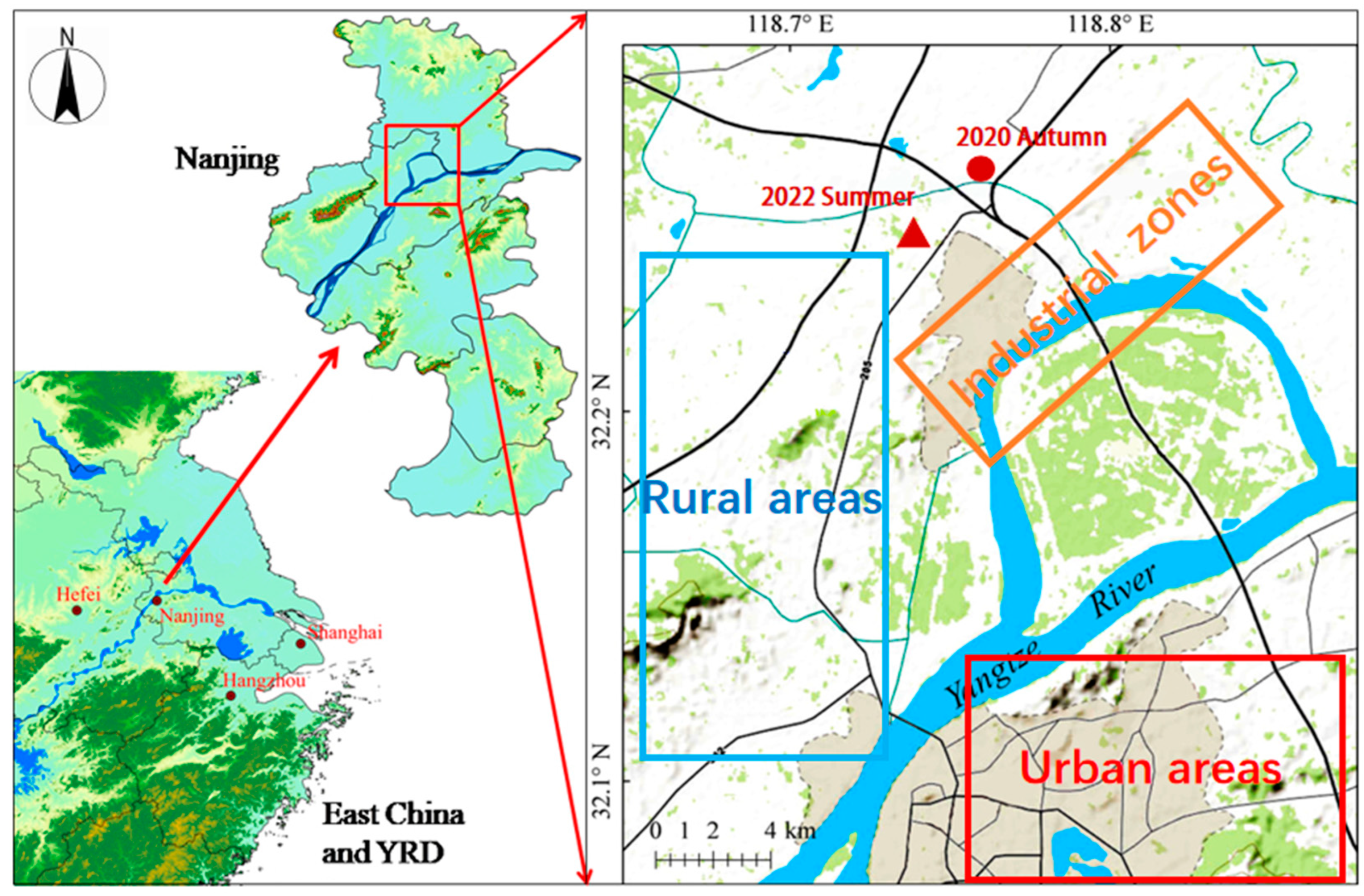
2.1.1. Observation Sites

The field campaigns in autumn of 2020 (32.26°N, 118.72°E) and summer of 2022 (32.23°N, 118.70°E) are located at the intersection of the industrial area and agricultural area in northern Nanjing. During the summer field observations, due to the impact of the COVID-19 pandemic, the original observation site unexpectedly closed. Consequently, we chose a new observation site located approximately 3.2 km away from the original site. Approximately 3.5 km to the east of the two observation points are the industrial parks, including steel, power generation, and chemical plants. The west is adjacent to the agricultural area. Approximately 15 km to the southeast is the Nanjing urban area. There are highways and transportation hubs within 1 km to the east and north. Their surrounding environment is shown in Figure 1.

The statistical analysis of meteorological parameters and surface concentrations of NO₂ and TVOCs at the observation sites during the summer and autumn is shown in

Table 1. Statistical characteristics of temperature, wind speed, NO₂, and VOCs during the observation period.

	Averaged		Standard Deviation		Maximum		Minimum
	Autumn	Summer	Autumn	Summer	Autumn	Summer	Autumn	Summer
Temperature (°C)	15.2	33.5	3.8	4.0	24.0	41.2	4.0	26.0
Wind speed (m/s)	2.2	2.8	1.3	1.7	7.0	8.0	0.3	0.2
NO2 (ppb)	30.9	8.4	13.7	3.9	45.3	18.7	4.9	1.3
TVOCs (ppb)	61.0	33.9	20.5	14.6	132.1	77.7	33.4	17.0

. During the autumn observation period, the average surface temperature and wind speed were 15.2 °C and 2.2 m/s, respectively, with prevailing winds from the northeast and northern directions. There was a significant difference in the daily variation of surface temperature and wind speed, with average standard deviations of 3.8 °C and 1.3 m/s, respectively. The average surface NO₂ concentration in autumn was 30.9 ppb, with a peak of 45.3 ppb occurring at 08:00 on November 7th. The average concentration of TVOCs at the surface in autumn was 61.0 ppb, with a maximum value of 132.1 ppb. During the summer observation period, the average surface temperature was 33.5 °C, which was 18.3 °C higher than in autumn, with a maximum temperature of 42.1 °C. The average wind speed was 2.8 m/s, with prevailing winds from the southwest. The average surface NO₂ concentration in summer was only 8.4 ppb, significantly lower than in autumn.

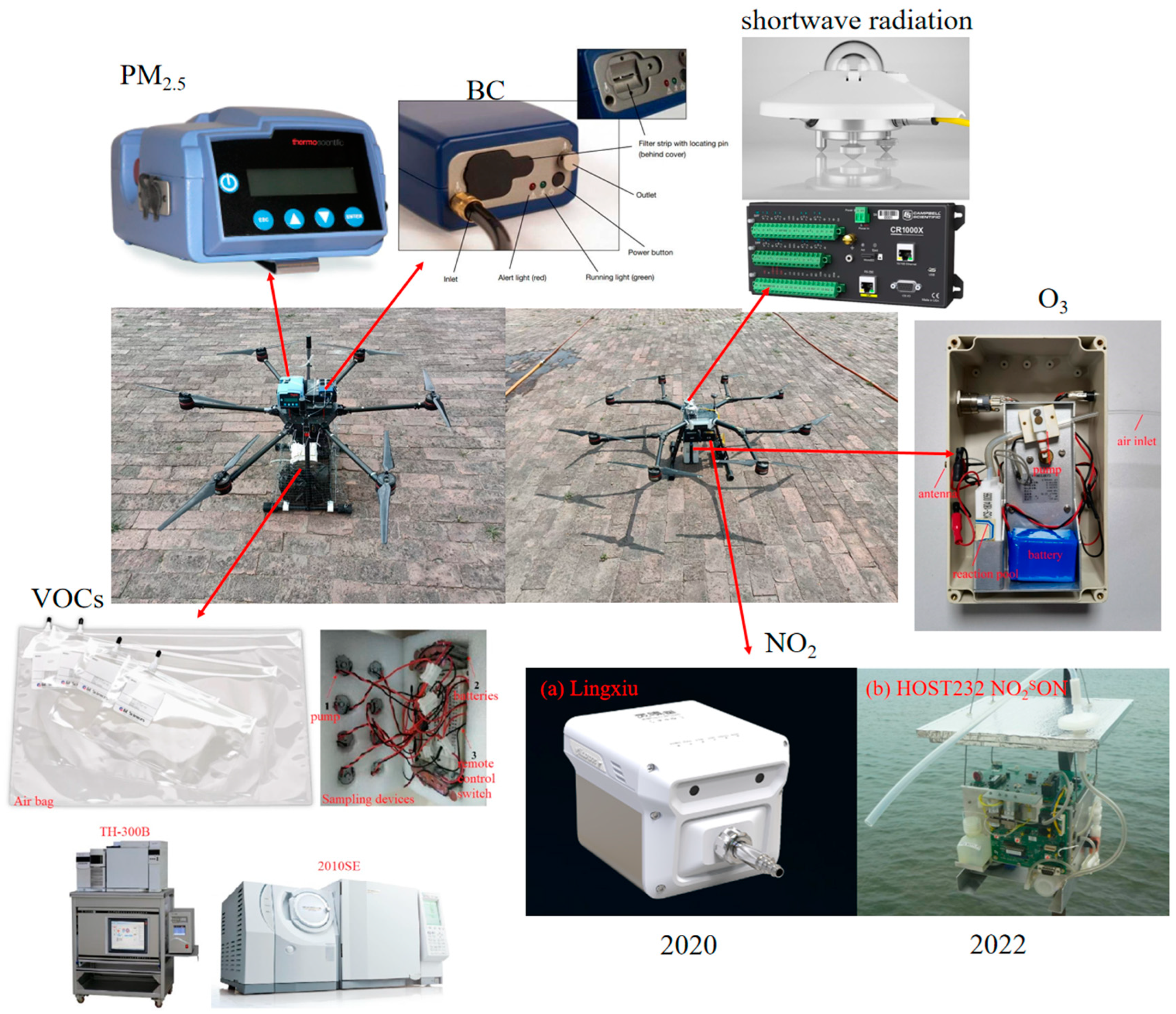
2.1.2. Observation Platforms, Instruments, and Sampling Methods

In the specific sampling process, this study relied on the UAV sounding system developed by the Institute of Atmospheric Physics, Chinese Academy of Sciences, which is mature and has been widely used in the Beijing-Tianjin-Hebei region [27,28] (Figure 2). The VOC detection system used in this study includes two independent modules: field collection and laboratory analysis. The VOC sampling device consists of 1-L Tedlar sampling bags (Shimadzu-GL, Tokyo, Japan) and a wireless remote-controlled miniature sampling pump, which are installed below the UAV. Sampling flights from the ground to a maximum altitude of 1 km were planned to take place at 08:00, 14:00, and 20:00 local time (LT) in the autumn of 2020 (18 October–15 November) and 06:00, 09:00, and 14:00 LT in the summer of 2022 (9–20 August). Ambient air was collected into Tedlar bags by corresponding pumps with a height resolution of 200 m, with each sample representing approximately ±100 m of air signature in the vertical direction [27,28,30]. Prior to field observations, the sampling bags were cleaned with high-purity nitrogen gas and evacuated with a vacuum pump to reduce measurement errors. At the same time, the bags were placed in black sunshade bags to reduce exposure to sunlight through the ground remote control system before flight. During the sampling process, the UAV platform carried the collection system and ascended at a constant speed of 2 m/s, sampling the air at the surface (approximately 2 m above ground) (before the UAV flight, air samples were collected at the ground level), 200 m, 400 m, 600 m, 800 m, and 1000 m. The air samples at different heights were collected by remotely controlling the pump switch. At different heights, air was pumped into different safety bags. The pump flow rate was 2 L/min, and the sampling time was approximately 1 min. The analysis module includes the TH-300B rapid online monitoring system for atmospheric VOCs produced by Wuhan Tianhong Environmental Protection Industry in China, and the gas chromatography-mass spectrometry/flame ionization detector (GS-MS/FID, 2010SE, Shimadzu-GL, Tokyo, Japan). After the field collection, all samples were sent to the laboratory for measurement in time. The time interval between sampling and testing was less than 36 h [44]. The daily collected samples were preconcentrated using the TH-300B system and then analyzed by GS-MS/FID. The analysis system has two channels, FID and MS. The air samples in the sampling bags enter the FID, where they are dehydrated and condensed at −50 °C, and then CO₂ is removed using a CO₂ absorption tube. Finally, C2–C5 hydrocarbons are captured by a PLOT capillary column at −150 °C. After entering the MS channel, the air samples are dehydrated and condensed at −20 °C, and then C6–C12 hydrocarbons and halocarbons are captured by a passivated air capillary column at −150 °C. The analysis procedures and detection limits of the tested compounds were the same as in the previous study [45,46,47]. The analysis module detected a total of 87 VOCs, 28 alkanes, 12 alkenes, 16 aromatics, and 30 halogenated hydrocarbons and acetylene. Due to the limitations of observation technology, this study did not comprehensively monitor formaldehyde and other OVOCs in the VOC observation experiment. The detailed components and corresponding detection limits can be found in the study conducted by Wu et al. [27,28].

During the autumn observation in 2020, the Lingxiu V1 instrument (Shenzhen Kefei Technology Co., Ltd., Shenzhen, China) was installed below the UAV to monitor the NO₂ concentration profile in real time, and the data was transmitted to the supporting software for analysis. Sampling flights from the ground to a maximum altitude of 1 km were conducted at 08:00, 14:00, and 16:00 local time (LT) in the autumn of 2020 (18 October 18–15 November); during the summer observation, the HOST232 NO₂^SON Tether Sonde (DRUMMOND TECHNOLOGY INC) was installed below the UAV to monitor the NO₂ concentration profile in real time. The primary display of the data was conducted using the HOST232 Windows program. The planned flight time and flight altitude of the UAV were consistent with the summer VOC observations. Both instruments are available to monitor real-time changes in NO₂ concentration and have demonstrated reliability and accuracy in NO₂ monitoring and have performed well in field tests [48,49,50].

In addition to the VOCs and NO₂ data mentioned above, GPS radiosondes also measured the vertical profiles of basic meteorological variables. This study utilized the wireless GPS radiosonde system developed by Nanjing Junquan Technology Co., Ltd. to vertically probe conventional meteorological elements. The GPS radiosonde system consists of a radiosonde instrument and a ground data-receiving system. The radiosonde instrument includes temperature and humidity modules, a pressure module, a GPS module, and a data transmission module, enabling the monitoring and transmission of data. The radiosonde instrument, carried aloft by a helium-filled balloon, can provide real-time vertical distribution data, including temperature, humidity, wind speed, wind direction, and pressure, which can be obtained through the ground receiving system. This radiosonde system exhibits high detection sensitivity, is virtually unaffected by weather conditions, and ensures data integrity. The temporal resolution of the meteorological data in this study is 1 s, with a maximum updraft of 3 m/s.

In the autumn of 2020, a total of 202 profiles were obtained from observations. Among them, there were 61 VOC profiles, 65 NO₂ profiles, and 76 meteorological profiles. In the summer of 2022, a total of 103 profiles were obtained from observations. Among them, there were 34 VOC profiles, 34 NO₂ profiles, and 35 meteorological profiles.

2.1.3. Quality Assurance and Quality Control

During sample analysis, the species measured by the FID detector (13 VOCs ranging from C2 to C5) are quantified using an external standard method. The species measured by the MS detector (79 VOCs ranging from C5 to C12) are quantified using the internal standard method, with real-time monitoring of quantitative changes in ion peak areas. Standard curves are constructed for 117 VOCs (consisting of PAMS (57 species), TO15 (65 species), and 13 aldehyde and ketone substances), where the relative standard deviation (RSD) of the target species’ relative response factors is less than 15%, and R2 > 0.98 [51]. After analyzing every 24 samples, the concentration of the second-highest point on the standard curve is analyzed to monitor whether the relative deviation of the measured results from the initial concentration values is less than 30%.

2.2. Observation Data and Methods

2.2.1. Observation Data Filtering

The original data from VOCs has problems, such as data discontinuity and outliers, so the original data needs to be processed. The principles are: (1) Remove wild points that are obviously beyond the reasonable range caused by human factors and instrument fluctuations; (2) remove missing observation data; and (3) remove individual peaks and singular peaks based on variance testing. The criteria are:

$$\left|X_i-X\right|>2.5\sigma$$

(1)

In the formula, $X_i$ is the measured value, $X$ is the average of the observed values, and $\sigma$ is the standard deviation. The vertical observation study by Lu et al. [52] used this principle for data processing. A total of 287 original samples were obtained during the autumn observation, and a total of 233 valid samples were retained after processing, accounting for 81% of the total samples. A total of 176 original samples were obtained during the summer observation, and a total of 139 valid samples were retained after processing, accounting for 79% of the total samples.

2.2.2. Calculation of BL NO₂ Vertical Column Concentration

Through in-situ observations, we can obtain the vertical profile of NO₂ concentration in the lower troposphere (with a resolution of 200 m). To further calculate the vertical column concentration of NO₂ in the BL based on this data, we used a simple numerical integration method for estimation. The calculation steps are as follows: first, we discretized the observed NO₂ concentration values by height, and then integrated them using the trapezoidal rule. Therefore, the formula for calculating the NO₂ column concentration in the BL is as follows:

$$\left\{BL {NO}_2 vertical column concentration\right\}={\sum }_{i=1}^n\frac{c_i+c_{i+1}}{2}\times ∆h$$

(2)

Here $c_i$ represents the NO₂ observed concentration at its height, $∆h$ is the difference between adjacent heights, and n is the number of height intervals. The obtained unit is ppb∙m, therefore, we further convert the unit to ×10¹⁶ molec/cm². The conversion formula is as follows:

$$c_{molec/{cm}^2}=c_{ppb·m}\times {10}^{-9}\times N_A$$

(3)

where N_A is Avogadro’s constant, approximately 6.022 × 10²³ molec/mol.

2.2.3. Calculation of the OH and NO₃ Loss Rates

The OH loss rate of VOCs, denoted LOH, provides an estimate of the initial formation rate of peroxyl radicals (RO₂). This peroxyl radical formation constitutes the rate-limiting step in atmospheric photochemical O₃ production. The value of LOH indicates the relative contribution of VOC species to daytime photochemical reactions. At night, the NO₃ radical is integral to atmospheric chemical cycles, governing the oxidation and removal of many trace gases. This substantially affects night-time SOA formation. The LNO₃ of VOCs signifies the relative role of VOC species in night-time SOA formation. Overall, LOH and LNO₃ reflect vertical changes in the reactivity of VOCs across daytime and night-time conditions. For the calculation of LOH and LNO₃, see Formulas (4)–(7).

$$LOH=\sum {\left[VOC\right]}_i\times K_i^{OH}$$

(4)

$$K_i^{OH}=A_1{T}^{n1}{e}^{-B_1/T}$$

(5)

$$L{NO}_3=\sum {\left[VOC\right]}_i\times K_i^{{NO}_3}$$

(6)

$$K_i^{{NO}_3}=A_2{T}^{n2}{e}^{-B_2/T}$$

(7)

where ${\left[VOC\right]}_i$ is the concentration of a certain VOC substance, $K_i^{OH}$ is the OH reaction constant of a certain VOC substance, $K_i^{{NO}_3}$ is the NO₃ reaction constant of a certain VOC substance, A₁, B₁, n1, A₂, B₂, and n2 are parameters that change with temperature, and T is the temperature [53].

2.3. Satellite Data Sources

2.3.1. TROPOMI

TROPOMI was launched aboard the European Space Agency’s (ESA) S5P spacecraft in October 2017. TROPOMI utilizes four spectral bands (ultraviolet, visible, near infrared, and shortwave infrared) to measure various atmospheric constituents like O₃, NO₂, carbon monoxide (CO), methane (CH₄), HCHO, and aerosols [54,55]. The visible band from 400 to 496 nm used for NO₂ retrieval has a spectral resolution of 0.54 nm sampled at 0.20 nm intervals and a signal-to-noise ratio of approximately 1500 [56]. HCHO retrieval employs the ultraviolet band spanning 320–405 nm [57].

TROPOMI features a push-broom configuration, covering a ~2600 km swath width on Earth’s surface. Most spectral bands have a typical pixel size of 7 km × 3.5 km near nadir, except for the UV1 band (7 km × 28 km) and shortwave infrared bands (7 km × 7 km). Compared to predecessor instruments like the Ozone Monitoring Instrument (OMI), TROPOMI’s higher spatial resolution and daily global coverage support enhanced observations of NO₂ and HCHO. Such fine-scale satellite measurements facilitate the analysis of localized spatiotemporal patterns in these species.

2.3.2. TROPOMI Observations Used in This Study

In this work, the near-real-time Level 2 NO₂ and HCHO tropospheric column data for the 2022 summer observation period (9–20 August) and the 2020 autumn observation period (18 October–15 November) were used [58,59,60]. The data from the Copernicus open data access hub https://browser.dataspace.copernicus.eu/, accessed on 5 December 2023. The near-real-time product available within 3 h after data acquisition can ensure the timeliness of data. Two additional versions of the data are available: the reprocessed version and an offline stream (available within a few days of collection).

In this study, the NO₂ and HCHO tropospheric vertical column concentrations retrieved from TROPOMI were redistributed, with the original pixels of approximately 7 × 3.5 km², setting to a newly defined 0.08° × 0.08° grid, centered on Jiangsu Province (southwest: 30°N, 116°E; north-east: 36°N, 123°E). After the original data were regridded, the data were averaged over different time frames, as described in Section 3.2.

3. Results

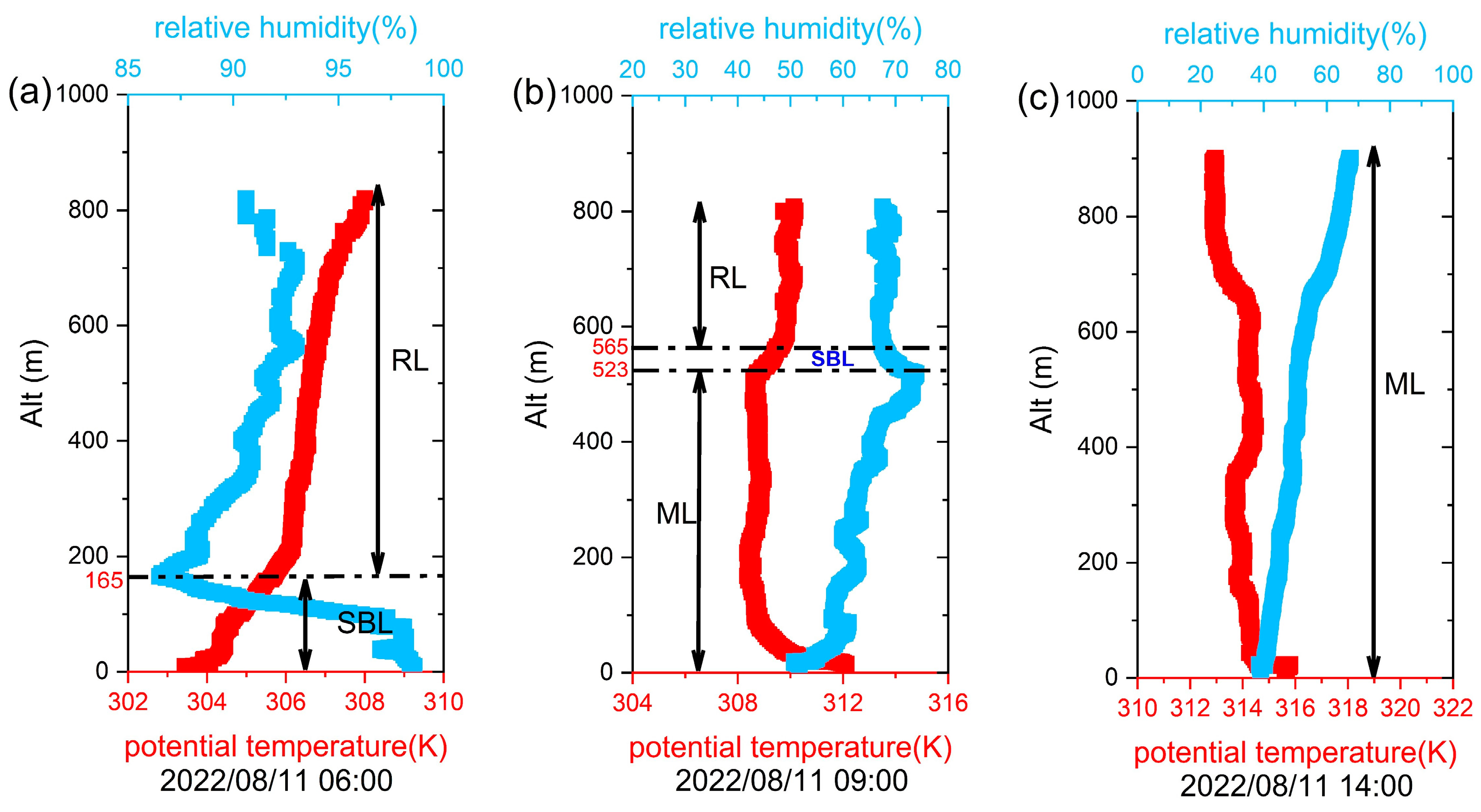
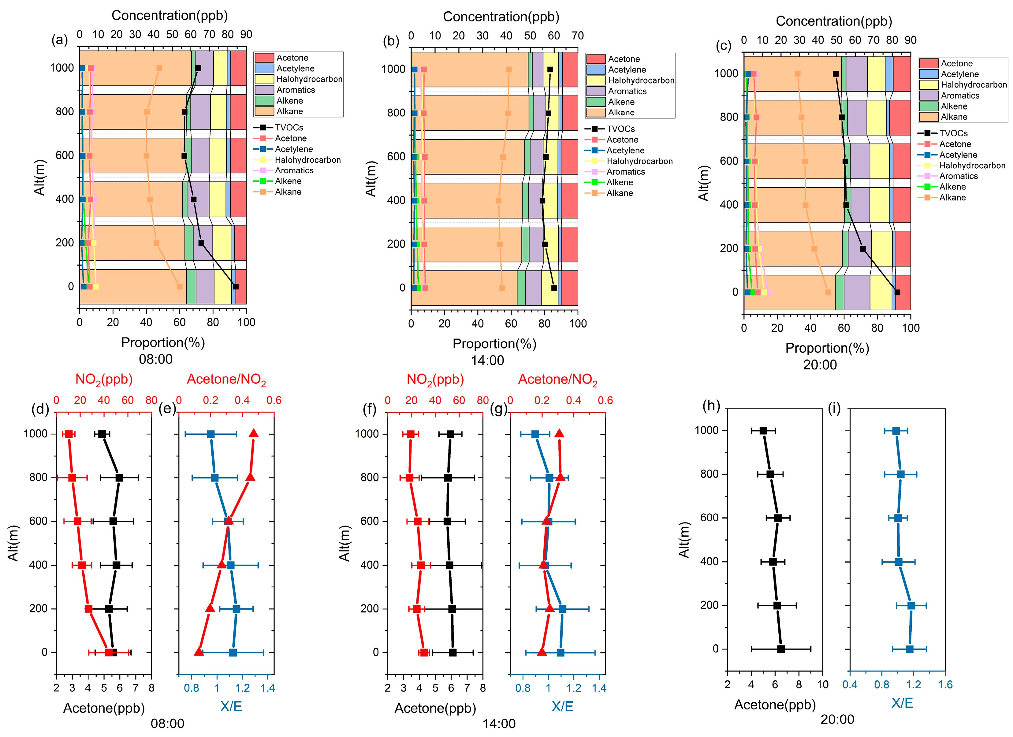
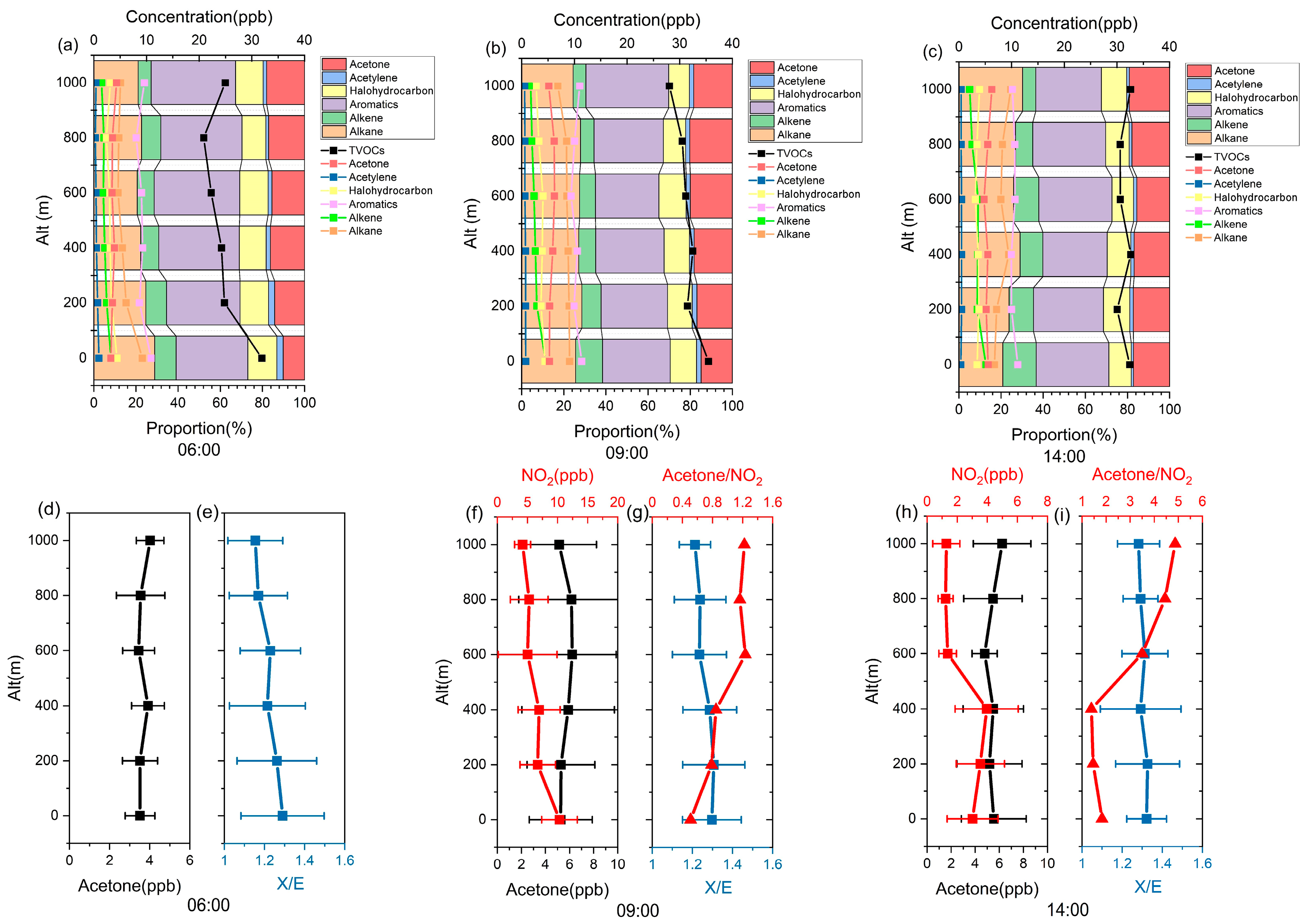
3.1. Thermal Layer Classification of BL and Characteristics of Vertical VOCs and NO₂

In this study, we classified the BL into a stable boundary layer (SBL), mixing layer (ML), and residual layer (RL) based on the diurnal evolution of potential temperature and relative humidity profiles [61]. Figure 3 provides an example explaining the criteria used to identify the BL thermal layers on 11 August 2022. In Figure 3a, in the early morning, the potential temperature below 165 m exhibited a notable increase with height, while the relative humidity decreased rapidly. These profiles were the persisting conditions of the night-time SBL conditions. Above 165 m, the profiles of potential temperature and humidity resembled those in the ML of the previous afternoon, and it was defined as the RL. In Figure 3b at 09:00, the potential temperature below 50 m decreased sharply with height as the result of surface heating by solar radiation. This layer was a super-adiabatic lapse rate layer. There were slight fluctuations in potential temperature and relative humidity from 50 m to 523 m, and it was defined as the ML from the surface to 523 m. Within the altitude range of 523–565 m, the potential temperature increased with height, concurrently accompanied by a decrease in relative humidity. This was characterized as a relatively shallow SBL zone. Above 565 m, the potential temperature and relative humidity changed gently with height, similar to that in the ML, likely retaining the ML characteristics of the previous afternoon, which was defined as the RL. In Figure 3c at 14:00, the potential temperature and relative humidity changed slightly, and the entire layer became a well-developed ML.

Figure 4a–c depict the diurnal variation of VOC average concentration profiles and the proportion of VOC species to TVOCs in autumn 2020. At 08:00, during rush hour, VOCs emitted from the surface accumulated in the shallow ML as they could not penetrate the upper SBL, reaching a maximum concentration of 84.3 ppb. The averaged concentration of TVOCs in the SBL dropped rapidly from 65.7 ppb at 200 m to 56.5 ppb at 600 m. The RL retained the vertical characteristics of VOCs from the previous day, exhibiting a relatively uniform distribution. As for the different VOC species, the distributions of alkanes and acetylene, both having low photochemical activity, followed similar profiles to TVOCs. In contrast, the alkenes with high photochemical activity were rapidly consumed at lower layers, as evidenced by decreasing mixing ratios (in ppb) and proportions to TVOCs with height. Although aromatic concentrations gradually decreased with height, their proportions were highest in the SBL (

Table 2. The averaged concentrations and proportions to TVOCs of VOC species in different layers of BL in summer and autumn (the values after the average concentrations represent plus or minus one standard deviation) (unit: ppb; %).

Autumn (2020)
	Alkane	Alkene	Aromatics	Acetylene	Acetone	TVOCs
ML	40.3 ± 18.0 (64.9%)	3.1 ± 2.4 (5.0%)	5.8 ± 2.7 (9.3%)	1.3 ± 0.8 (2.1%)	5.5 ± 1.1 (8.8%)	62.1 ± 21.8
SBL	37.9 ± 14.9 (60.4%)	2.5 ± 1.7 (4.0%)	8.1 ± 4.8 (12.9%)	1.6 ± 1.0 (2.6%)	5.9 ± 1.8 (9.4%)	62.7 ± 20.0
RL	38.3 ± 16.8 (64.0%)	1.9 ± 1.4 (3.2%)	6.2 ± 2.4 (10.4%)	1.3 ± 0.8 (2.2%)	6.0 ± 1.9 (10.0%)	59.9 ± 19.4
Summer (2022)
ML	8.3 ± 5.7 (26.1%)	3.5 ± 3.1 (11.0%)	10.5 ± 5.9 (33.0%)	0.5 ± 0.3 (1.6%)	5.4 ± 2.5 (17.1%)	31.9 ± 13.8
SBL	7.8 ± 3.0 (27.5%)	2.9 ± 1.5 (10.1%)	9.9 ± 5.4 (34.7%)	0.6 ± 0.3 (2.0%)	3.4 ± 1.1 (11.8%)	28.6 ± 8.6
RL	6.9 ± 5.0 (23.9%)	2.3 ± 1.6 (8.0%)	10.9 ± 7.3 (37.9%)	0.5 ± 0.3 (1.6%)	5.0 ± 3.3 (17.4%)	28.8 ± 14.1

). The proportion of acetone, primarily derived from VOC oxidation [39,40], gradually increased with height. At 14:00, the entire lower troposphere comprised the ML with good vertical diffusion, and VOC species were evenly distributed. At 20:00, the suppressed turbulence in nocturnal SBL hindered upward VOC diffusion. Thus, the surface TVOC concentration was relatively high, up to 82.8 ppb, while VOC species were evenly distributed in the RL.

The oxidation processes of VOCs in the atmosphere can be described by the variations in specific VOC species ratios that have the same sources but notably different photochemical activities. VOC species with higher reactivity were more easily oxidized by OH radicals than those with lower reactivity. Therefore, the ratio of highly reactive species concentration to low reactive species concentration was the largest in fresh emitted air masses and became smaller as the air mass aged [29,62]. In this study, we utilized the ratio of m,p-xylene concentration to ethylbenzene concentration to characterize the aging degree of the air mass. Their respective rate constants are 1.87 × 10⁻¹¹ and 7.0 × 10⁻¹² cm³ molecule⁻¹ s⁻¹, respectively, representing a 2.7 times difference in reactivity. Furthermore, m,p-xylene and ethylbenzene were highly correlated, with correlation coefficients of 0.98 and 0.96 in the autumn and summer, respectively. Figure 4e,g,i illustrate m,p-xylene/ethylbenzene ratio variations with height in the autumn of 2020. At 08:00, the m,p-xylene/ethylbenzene ratio significantly decreased from 1.13 at ground level to 0.95 at 1000 m, which indicated significant aging in the RL. At 14:00, the m,p-xylene/ethylbenzene ratio overall decreased with height, albeit with weaker gradients. At 20:00, the m,p-xylene/ethylbenzene ratio peaked in the SBL, with no discernible change in the RL but significantly smaller ratios than the SBL. In summary, the diurnal changes in m,p-xylene/ethylbenzene ratio profiles indicated that active species in freshly emitted VOCs from the surface were rapidly oxidized and depleted during vertical diffusion, and the air mass was more aged in the upper of the BL compared to the lower layer.

Previous studies have indicated that acetone mainly comes from the secondary generation of VOCs [63], while NO₂ is mainly directly emitted. Therefore, the acetone/NO₂ concentration ratio can also be used to characterize the oxidation consumption of VOCs and the generation of OVOCs. The greater the value of acetone/NO₂, the greater the oxidation consumption of directly emitted VOCs and the greater the generation of OVOCs. Figure 4d,f,h present NO₂ and acetone concentration profiles, and Figure 4e,g,i depict acetone/NO₂ ratio variations with height in the autumn of 2020. At 08:00, NO₂ concentrations rapidly decreased, whereas acetone initially increased, then decreased with height, exhibiting two concentration peaks at 400 m and 800 m. The acetone/NO₂ ratio gradually increased from 0.13 on the ground to 0.47 at 1000 m. At 14:00, NO₂ concentrations slowly declined with height, while acetone remained constant. The acetone/NO₂ ratio exhibited an overall increasing trend with height.

Figure 5a–c depict the diurnal variations of VOC averaged concentration profiles and the proportions of VOC species to TVOCs in summer 2022. At 06:00, the presence of the nocturnal SBL inhibited the upward diffusion of VOCs, resulting in relatively elevated surface TVOC concentrations of 31.9 ppb. From 200 m to 800 m, VOC species concentrations gradually decreased, with a subtle elevation observed at 1000 m, potentially due to long-range transport of air pollutants [27,28]. At 09:00, VOCs had accumulated in the ML and SBL, culminating in a maximum surface concentration of 35.5 ppb. The concentration profiles of VOCs exhibited marginal changes from 200 m to 600 m, with a gradual decline observed above 600 m (in the RL). At 14:00, the concentration profiles of individual VOC species exhibited insignificant variations with respect to height. It was worth noting that easterly winds potentially contributed to marginally elevated TVOCs at 400 m, as the sampling position was being influenced by fresh emissions from the high stack sources to the east in the nearby industrial zone (see description of the measurement sites).

In addition to diurnal fluctuations, the concentrations and species composition of VOCs exhibited significant variations in the three thermal layers of summer and autumn. Table 2 illustrates that overall, the TVOC concentration in the autumn was notably higher (50%) than that in the summer. Moreover, the proportions of alkanes were predominant during the autumn, whereas the proportions of aromatics prevailed during the summer. Despite substantial disparities in both concentrations and species compositions of VOCs, similar trends were observed in the concentration levels and proportions of VOC species across the three layers during the two seasons. Specifically, the proportions of less reactive alkanes and acetylene remained relatively consistent in ML, SBL, and RL. In contrast, alkenes demonstrated high photochemical reactivity and oxidized faster than inactive VOCs like alkanes, resulting in notable proportional differences across layers. In autumn and summer, alkenes accounted for 5.0% and 11.0% in the ML, but only 3.2% and 8.0% in the RL. It was noteworthy that the proportion (12.9%) of aromatics peaked in the nocturnal SBL in autumn due to VOCs emitted by steel and chemical companies around the observation site at night. While the proportion (37.9%) of aromatics peaked in RL in the summer, as a secondary oxidation product, acetone proportions gradually increased with height, reaching maximums of 10.0% and 17.4% in the autumn and summer RL, respectively.

Comparing the m,p-xylene/ethylbenzene ratio profiles in summer and autumn (Figure 4e,g,i and Figure 5e,g,i), it can be seen that the ratios in autumn were larger and demonstrated more pronounced vertical gradient changes compared to summer. For instance, between 08:00 and 09:00, the m,p-xylene/ethylbenzene ratio in autumn decreased from 1.13 at the ground to 0.95 at 1000 m, while in summer it only decreased from 1.30 to 1.21. As discussed previously, the smaller m,p-xylene/ethylbenzene ratio indicates a more aged air mass. Consequently, the degree of air mass aging was notably higher in the autumn compared to the summer. Analyzing the diurnal characteristics of m,p-xylene/ethylbenzene ratio profiles in the summer of 2022 (Figure 5e,g,i), it was evident that at 06:00, the concentration ratio was highest in the nocturnal SBL and markedly lower in the RL, with the m,p-xylene/ethylbenzene ratio decreasing from 1.29 at the surface to 1.15 at 1000 m. At 09:00, the m,p-xylene/ethylbenzene ratio peaked in the ML, decreased markedly in the SBL, and exhibited minimal changes in the RL, similar to that in the autumn. At 14:00, the m,p-xylene/ethylbenzene ratio exhibited negligible variation with height.

The photolysis rate of NO₂ is contingent upon the intensity of solar radiation, with heightened solar radiation resulting in accelerated NO₂ photolysis [64,65]. Comparing the acetone/NO₂ ratio profiles in summer and autumn, it was evident that the gradient of the ratio increase at 14:00 was more pronounced in the summer than in the autumn. In the autumn, the acetone/NO₂ ratio increased from 0.20 at ground level to 0.31 at 1000 m (1000 m was 1.6 times of that at the ground), while in the summer it increased from 1.83 to 4.87 (1000 m was 2.7 times of the ground). This disparity may be attributed to the intense solar radiation experienced in the upper and middle layers of the BL and rapid NO₂ consumption on summer afternoons. Analyzing the diurnal variations of NO₂ and acetone concentration profiles as well as acetone/NO₂ ratio profiles in summer 2022 (Figure 5d–i), in the daytime (at 06:00, 09:00, and 14:00), acetone concentrations overall increased with height, while NO₂ concentrations sharply decreased. At 09:00, the acetone/NO₂ ratio markedly increased from 0.51 at ground level to 1.22 at 1000 m, indicating significantly higher secondary VOC oxidation in the upper layers compared to the lower layers. At 14:00, NO₂ rapidly decreased, leading to a marked rise in acetone/NO₂ ratio from 1.39 at 400 m to 3.50 at 600 m.

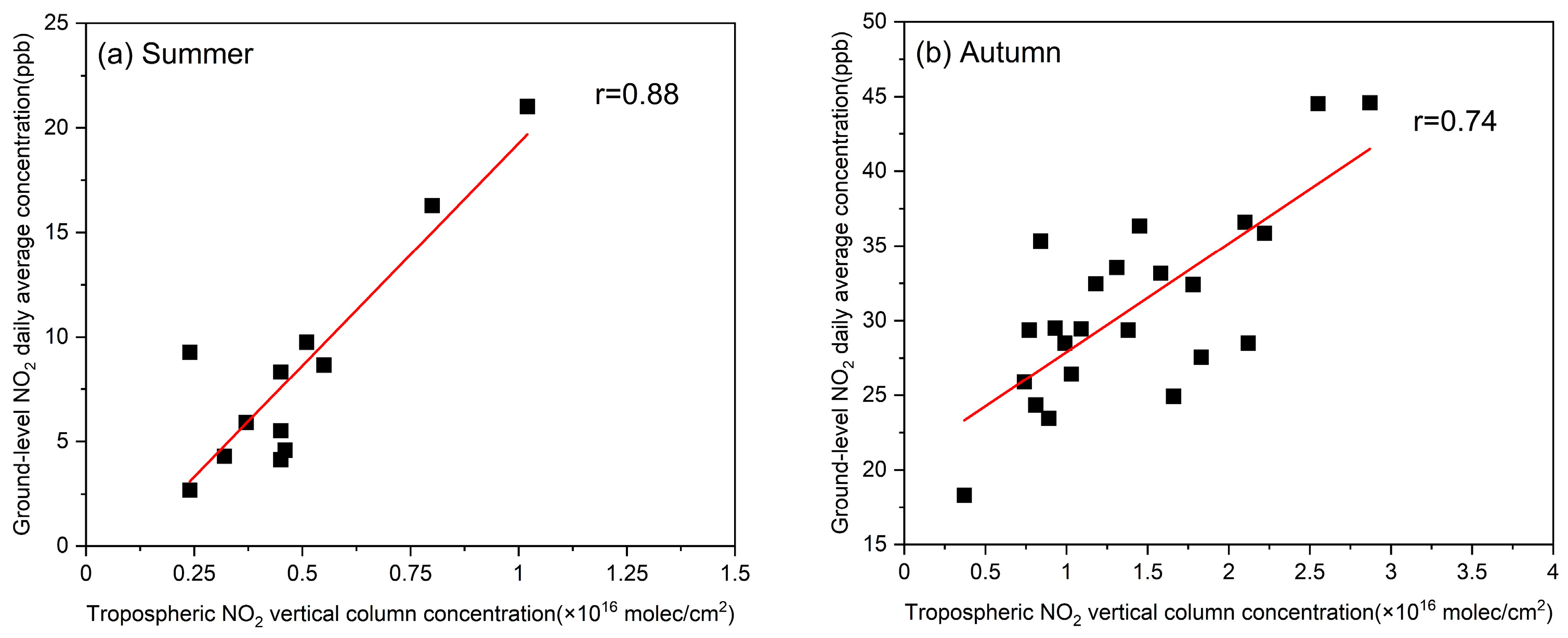
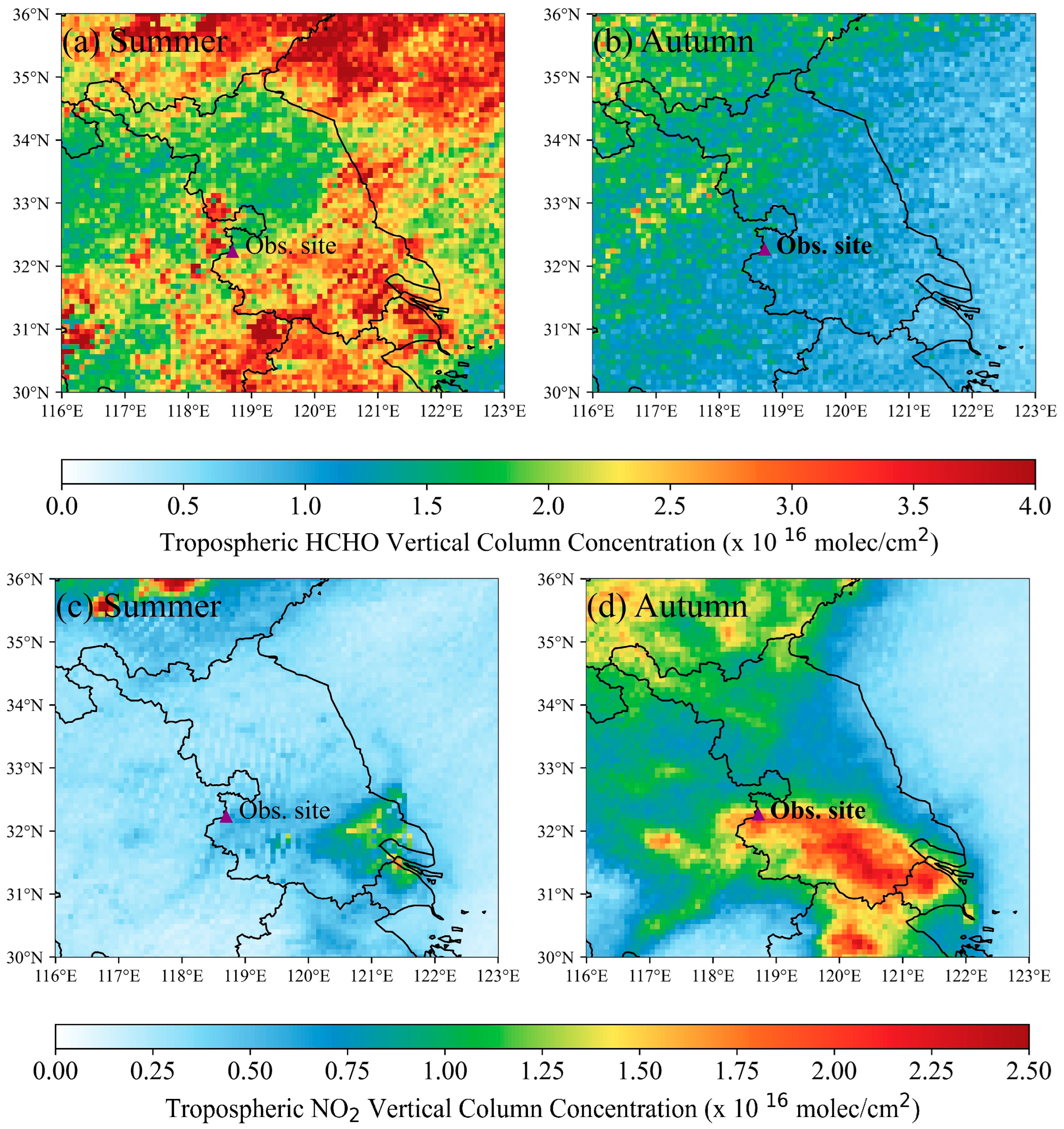
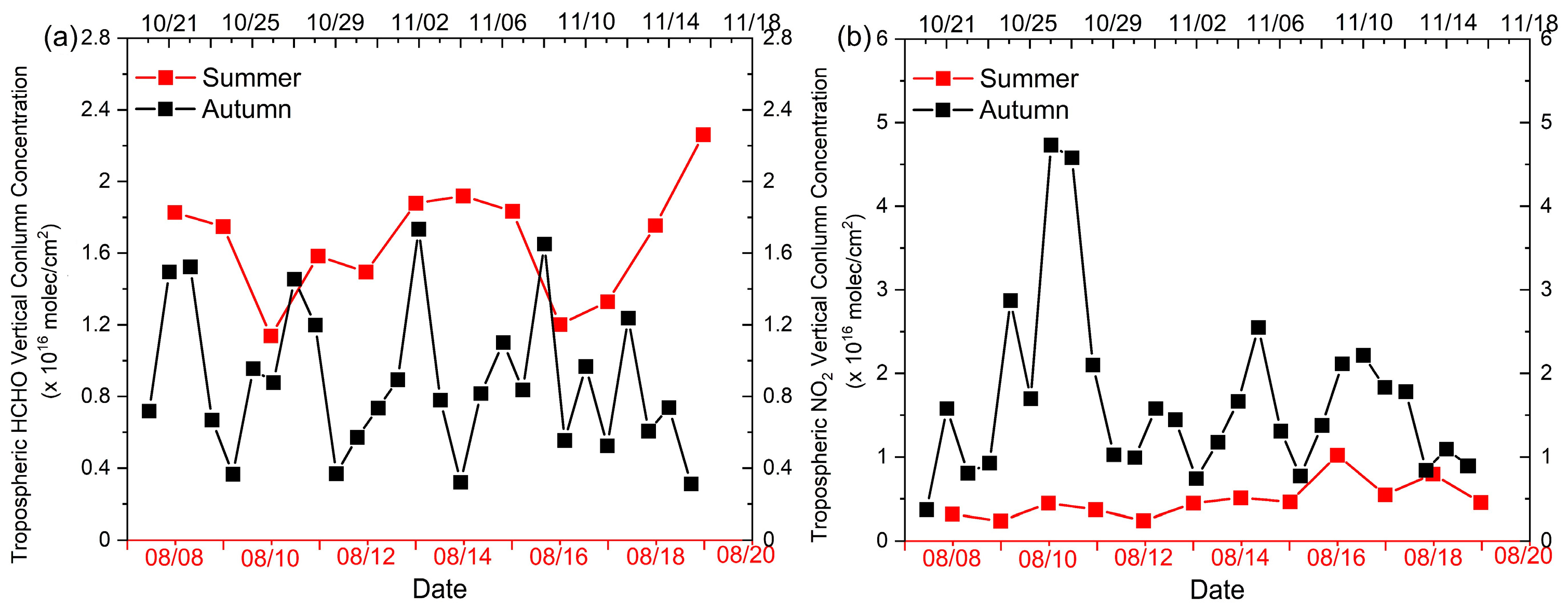
3.2. Satellite Data and Observations

This study analyzed seasonal differences in NO₂ and OVOCs (ketones and aldehydes) concentrations at observation points based on TROPOMI satellite retrieval data and in-situ observation data. The averaged HCHO tropospheric vertical column concentration in the summer was 1.82 (×10¹⁶ molec/cm²), while in autumn it was 0.89 (×10¹⁶ molec/cm²), 2.0 times higher than autumn (Figure 6 and Figure 7). The averaged surface acetone concentration from our in-situ observations was slightly higher in the summer (6.06 ppb) than autumn (5.78 ppb), like the seasonal differences in OVOCs shown in the TROPOMI satellite retrieval. In contrast, the NO₂ tropospheric vertical column concentration was higher in the autumn than that in the summer. The autumn and summer averages were 1.66 (×10¹⁶ molec/cm²) and 0.50 (×10¹⁶ molec/cm²), respectively. Correspondingly, the averaged surface NO₂ concentrations were 30.89 ppb in autumn and only 8.38 ppb in summer. This may be attributed to the stronger solar radiation in the summer than autumn resulted in faster NO₂ photolysis and rapid reactive consumption in the troposphere.

Furthermore, in order to further validate the credibility of our research by better integrating observational data and satellite data, we analyzed the correlation between the tropospheric NO₂ vertical column concentration derived from satellite retrieval and the ground-level NO₂ daily average concentration obtained from our in-situ observations during the summer and autumn seasons. The correlation coefficients between the tropospheric NO₂ vertical column concentration and the ground-level NO₂ daily average concentration were 0.88 and 0.74 (p < 0.05) in the two seasons, respectively, as shown in Figure 8. These two types of data exhibit a good correlation. Additionally,

Table 3. Statistical results of the tropospheric NO₂ vertical column concentration, the NO₂ vertical column concentration in the BL, and its proportion to the total tropospheric vertical column concentration.

Autumn (2020)
Dates	1020	1022	1023	1024	1028	1029	1030	1031	1102	1103	1104	1105
Tropospheric NO2 vertical column (×1016 molec/cm2)	0.37	0.81	0.93	2.87	2.10	1.03	0.99	1.58	0.74	1.18	1.66	2.55
BL NO2 vertical column (×1016 molec/cm2)	0.21	0.34	0.37	1.64	1.44	0.55	0.56	0.89	0.37	0.52	1.06	1.49
BL/Tropospheric (%)	56.76	41.98	39.78	57.14	68.57	53.40	56.57	56.33	50.00	44.07	63.86	58.43
dates	1106	1108	1109	1110	1111	1112	1114	1115	Averaged
Tropospheric NO2 vertical column (×1016 molec/cm2)	1.31	1.38	2.12	2.22	1.83	1.78	1.09	0.89
BL NO2 vertical column (×1016 molec/cm2)	0.93	0.85	1.02	1.48	1.32	0.89	0.72	0.39
BL/Tropospheric (%)	70.99	61.59	48.11	66.67	72.13	50.00	66.06	43.82	55.87
Summer (2022)
dates	0808	0810	0811	0812	0813	0814	0815	0816	0817	0818	0819	Averaged
Tropospheric NO2 vertical column (×1016 molec/cm2)	0.32	0.45	0.37	0.24	0.45	0.51	0.46	1.02	0.55	0.80	0.45
BL NO2 vertical column (×1016 molec/cm2)	0.21	0.28	0.19	0.09	0.12	0.34	0.24	0.57	0.27	0.43	0.16
BL/Tropospheric (%)	65.63	62.22	51.35	37.50	26.67	66.67	52.17	55.88	49.09	53.75	35.56	50.59

provides the tropospheric NO₂ column concentration, the NO₂ column concentration in the BL, and their proportion. Excluding some outliers, during the observation periods in summer and autumn, the average proportion of BL NO₂ vertical column concentration to the tropospheric NO₂ vertical column concentration exceeded 50% in both seasons, reaching 50.6% and 55.9% in the summer and autumn, respectively. The maximum proportion in autumn was 72.1%, and in summer it was 66.7% (Table 3). This indicated that the NO₂ vertical column concentration in the BL accounted for a significant portion of the entire tropospheric vertical column concentration.

In addition to direct emissions, acetone and HCHO, as typical OVOC species, are largely produced from the secondary oxidation of VOCs. In contrast, the vertical distribution of NO₂ is influenced by surface emissions and turbulent diffusion [66]. It was previously noted that the lower troposphere acetone/NO₂ ratio increased with altitude (Figure 4 and Figure 5). Similar conclusions have been found in many studies investigating vertical OVOCs and NO₂ profiles based on in-situ observational or satellite-retrieval data [67,68,69,70,71,72]. For example, Jin et al. [68] found an overall smaller vertical decrease for HCHO compared to NO₂ based on satellite-retrieval data. Souri et al. [71] also found that NO₂ concentrations tend to decrease faster than HCHO from the surface to 5.75 km (including the boundary layer and midfree troposphere), and the HCHO/NO₂ ratio increased with altitude below 1.5 km. From the atmospheric pollutant vertical observation study conducted by Wang et al. [72], we can also conclude that within the range from the ground to 1 km, NO₂ concentration decreased by more than 80%, while HCHO concentration decreased by approximately 30%. The gradient of NO₂ concentration decrease in the lower troposphere was much greater than that of HCHO.

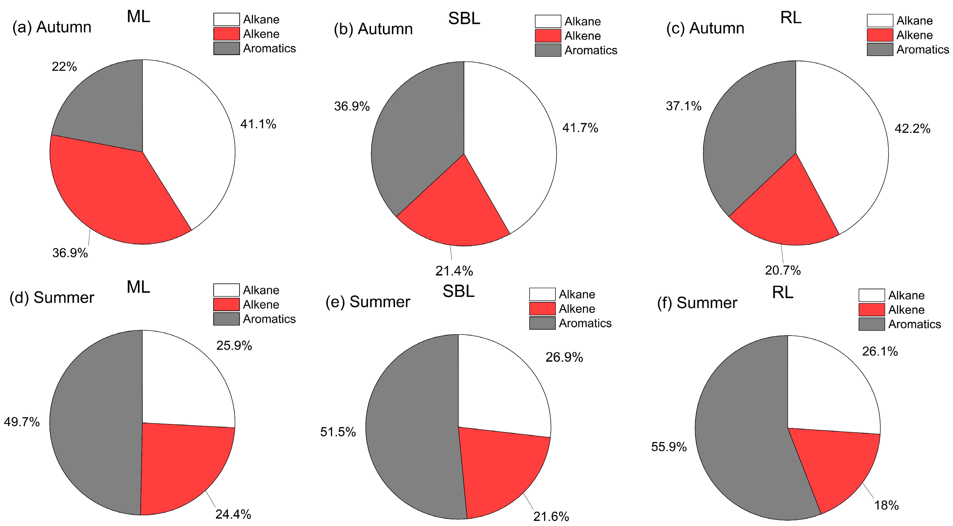
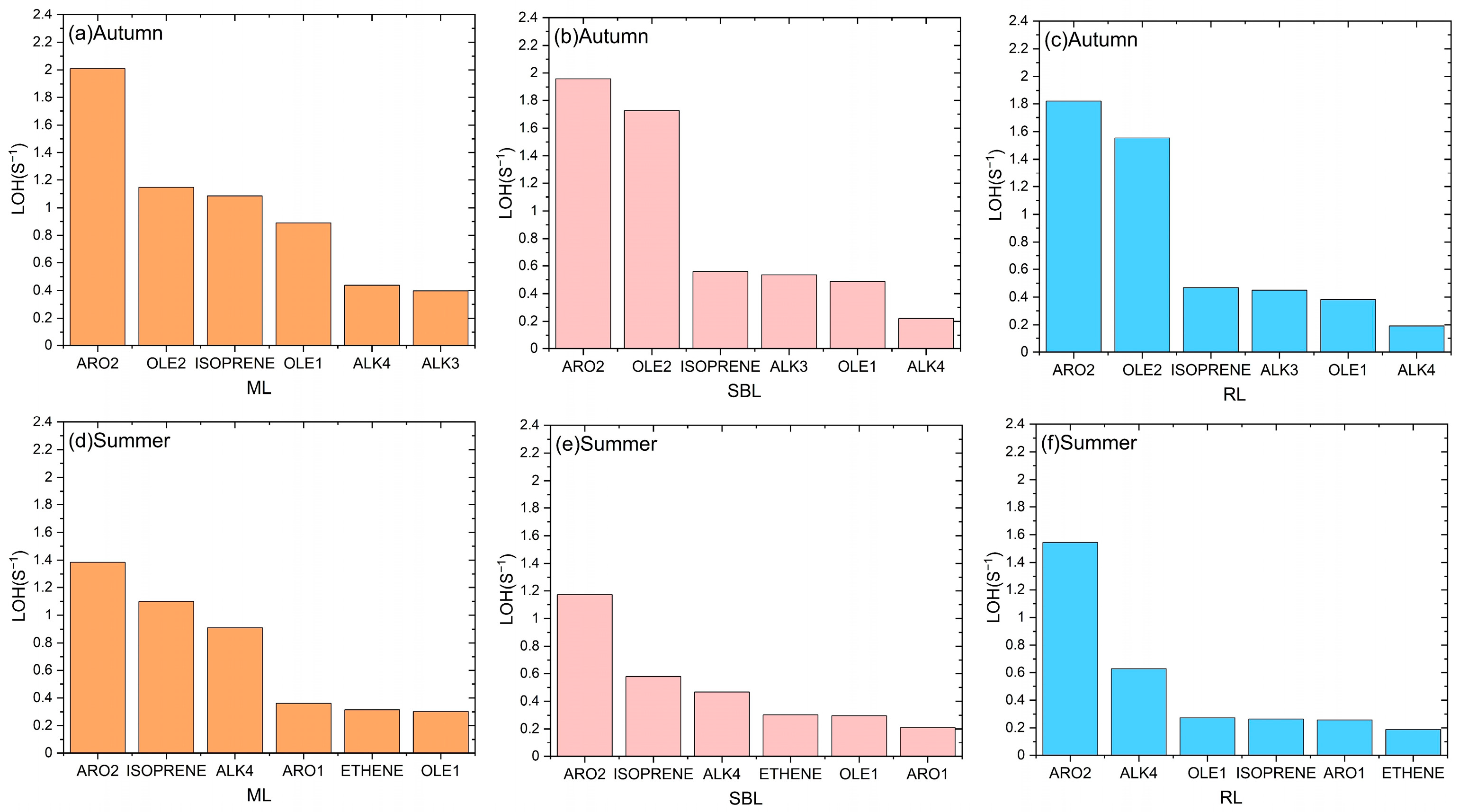
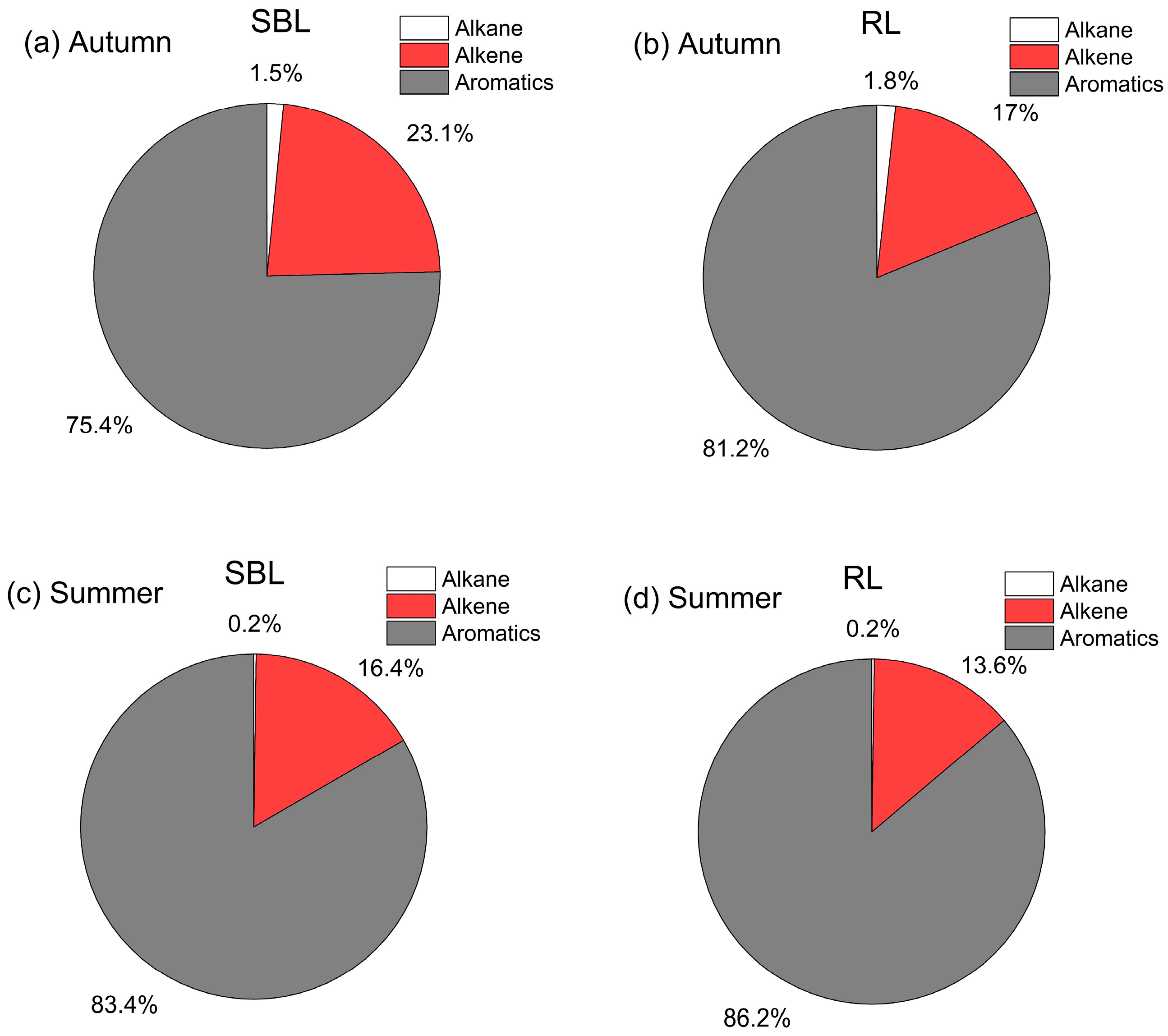
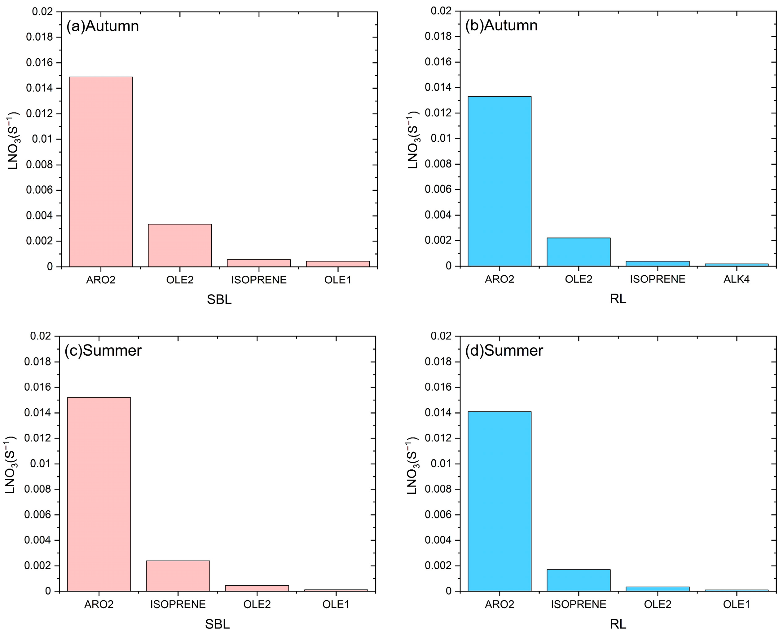
3.3. Differences in VOC Photochemical Reactivity in Different Layers

During the daytime, atmospheric OH radicals engage in reactions with VOCs to produce RO₂, which is the rate-determining step for photochemical O₃ formation. Various VOC species exhibit distinct photochemical reactivity with OH radicals. Consequently, the LOH measures the relative contribution of VOC species to daytime O₃ generation; a higher LOH of VOC species denotes a greater contribution to O₃ production [73]. Similarly, at night in the SBL and RL, O₃ reacts with NO₂ to yield NO₃ radicals, which degrade VOCs to form SOA [74]. Since NO₃ radicals are key in night-time atmospheric chemistry, the LNO₃ indicates the relative VOC species contribution to night-time SOA formation. As delineated by the relevant equations, LOH or LNO₃ of the VOC species equals the product of its concentrations and its reaction rate constant with OH (KOH) or NO₃ (KNO₃), respectively. Subsequently, we aim to elucidate the contribution of the main VOC species (alkanes, alkenes, and aromatics) in different layers of BL during the daytime to photochemical O₃ generation and at night to SOA generation.

Table 4. The averaged LOH of VOC species in different layers during the day in summer and autumn (units: s⁻¹).

Autumn (2020)
	Alkane (s−1)	Alkene (s−1)	Aromatics (s−1)	LOH (s−1)
ML	2.8 ± 0.6	2.6 ± 1.3	1.5 ± 0.7	6.9 ± 1.3
SBL	2.6 ± 0.4	1.3 ± 0.3	2.3 ± 0.4	6.3 ± 0.9
RL	2.3 ± 0.4	1.1 ± 0.2	2.0 ± 0.5	5.5 ± 0.8
Summer (2022)
ML	1.3 ± 0.3	1.2 ± 0.4	2.5 ± 0.7	5.0 ± 1.1
SBL	1.1 ± 0.2	0.9 ± 0.2	2.2 ± 0.5	4.3 ± 0.6
RL	1.0 ± 0.1	0.7 ± 0.3	2.2 ± 0.3	4.0 ± 0.7

and Figure 9 present the averaged LOH and proportions for VOC species in different layers of BL during the daytime in the summer and autumn. Overall, autumnal LOH exceeded summer values by approximately 40% in all layers. This discrepancy primarily stems from the 50% higher TVOC concentration in the autumn compared to the summer, despite lower ratios of active VOCs in the autumn. Additionally, there were distinct differences in LOH in different layers of BL, with maximal values in the ML for both seasons (6.9 s⁻¹ and 5.0 s⁻¹ in the summer and autumn, respectively), followed by the SBL (6.3 s⁻¹ and 4.3 s⁻¹ in the summer and autumn, respectively). The RL exhibited the lowest LOH (5.5 s⁻¹ and 4.0 s⁻¹ in the summer and autumn, respectively). These differences indicated that the VOCs in ML contributed the greatest potential photochemical reactivity and O₃ production during daytime than that in SBL and RL. Combining the data in Table 2, the averaged concentrations of VOCs in ML were greater than those in RL, and the concentrations and proportions of active species (e.g., alkenes) in RL were the lowest. For example, the alkene concentration in RL in autumn was only 1.9 ppb, which was 38.7% less than that in ML. Therefore, VOCs in RL had the smallest potential contribution to O₃ generation.

Specifically, for alkanes, their LOH and proportion exhibited minimal variations among the three thermal layers of BL. In autumn, the LOHs of alkanes were 2.8, 2.6, and 2.3 s⁻¹ in the ML, SBL, and RL, respectively (approximately 41–42% of total LOH). Due to substantially higher alkane concentrations relative to other VOC species, their proportion of total LOH was highest in all layers. Similarly, in the summer, the LOHs of alkanes were 1.3, 1.1, and 1.0 s⁻¹ in the ML, SBL, and RL, respectively (approximately 26% of total LOH). The LOHs of alkenes were 2.6, 1.3, and 1.1 s⁻¹ in the ML, SBL, and RL in the autumn, respectively, and the proportion decreased rapidly from 36.9% in the ML to 20.7% in the RL. The LOHs of alkenes were 1.2, 0.9, and 0.7 s⁻¹ in the ML, SBL, and RL in the summer, respectively, with the largest proportion in the ML (24.4%) and the smallest proportion in the RL (only 18.0%). The contribution of alkenes to photochemical reactions was highest in the ML during the daytime, indicating that alkanes were more effective in the generation of photochemical O₃. This was mainly because the ML was greatly affected by surface emissions, and the proportions of alkenes in the ML were highest at 11.0% and 5.0% in summer and autumn, respectively. Meanwhile, the more aged air in the SBL and RL had lower proportions of alkenes, at only 8.0% and 3.2% in the summer and autumn, respectively, resulting in less contribution to O₃ generation in the RL and SBL. The LOH and proportion of aromatics were higher in the SBL and RL compared to the ML. During autumn, the proportion of aromatic LOH peaked at 36.9% in the SBL but comprised only 22.0% in the ML. In the summer, aromatics accounted for the maximum LOH (55.9%) in the RL and the minimum (49.7%) occurring in the ML, which indicated that aromatics were the primary species contributing to photochemistry and O₃ generation in the SBL and RL.

As for the LOH of specific VOC species, we further subdivided alkanes, alkenes, and aromatics into species based on the SAPRC chemical mechanism to explore the main VOC contributors to daytime photochemical O₃ generation and night-time SOA generation in different layers of BL. The SAPRC chemical mechanism mainly divides VOCs through the reactivity of VOC species and OH radicals. Specifically, for alkanes, there are five categories: ALK1 (200 ppmv⁻¹ min⁻¹ < KOH < 500 ppmv⁻¹ min⁻¹), ALK2 (500 ppmv⁻¹ min⁻¹ < KOH < 2500 ppmv⁻¹ min⁻¹), ALK3 (2500 ppmv⁻¹ min⁻¹ < KOH < 5000 ppmv⁻¹ min⁻¹), ALK4 (5000 ppmv⁻¹ min⁻¹ < KOH < 10,000 ppmv⁻¹ min⁻¹), and ALK5 (KOH > 10,000 ppmv⁻¹ min⁻¹). Alkenes are classified into four groups: ETHENE, ISOPRENE, OLE1 (KOH < 70,000 ppmv⁻¹ min⁻¹), and OLE2 (KOH > 70,000 ppmv⁻¹ min⁻¹). Lastly, aromatics are categorized into three types: BENZENE, ARO1 (KOH < 20,000 ppmv⁻¹ min⁻¹), and ARO2 (KOH > 20,000 ppmv⁻¹ min⁻¹) [52,75]. In Figure 10, it was found that the top three VOC species contributing to LOH in the three layers of BL in autumn were all ARO2, OLE2, and ISOPRENE. The sum of the top three VOC species LOH accounts for more than 60% of the total LOH in each layer. In summer, the top three VOC species contributing to LOH were ARO2, ISOPRENE, and ALK4 in the ML and SBL. In the RL, they were ARO2, ALK4, and OLE1.

Table 5. The averaged LNO₃ of VOC species in different layers at night in summer and autumn (units: s⁻¹).

Autumn (2020)
	Alkane (s−1)	Alkene (s−1)	Aromatics (s−1)	LNO3 (s−1)
SBL	3.1 × 10−4 ± 0.6 × 10−4	4.6 × 10−3 ± 1.1 × 10−3	1.5 × 10−2 ± 0.5 × 10−2	2.0 × 10−2 ± 0.5 × 10−2
RL	2.9 × 10−4 ± 0.9 × 10−4	2.8 × 10−3 ± 0.8 × 10−3	1.3 × 10−2 ± 0.4 × 10−2	1.6 × 10−2 ± 0.3 × 10−2
Summer (2022)
SBL	4.1 × 10−5 ± 0.7 × 10−5	3.0 × 10−3 ± 0.4 × 10−3	1.5 × 10−2 ± 0.3 × 10−2	1.9 × 10−2 ± 0.5 × 10−2
RL	3.9 × 10−5 ± 0.3 × 10−5	2.2 × 10−3 ± 0.3 × 10−3	1.4 × 10−2 ± 0.4 × 10−2	1.7 × 10−2 ± 0.4 × 10−2

and Figure 11 show the averaged LNO₃ and proportions for VOC species in the SBL and RL at night during the summer and autumn. There was no ML at night. In general, the LNO₃ in the two layers had no significant seasonal differences. In the autumn, LNO₃ in the SBL was approximately 5% higher than that in the summer, while LNO₃ in the RL was approximately 6% lower than that in the summer. It was worth noting that the LNO₃ in the SBL was higher than the RL in both seasons, indicating that VOCs in the SBL contributed more to the formation of SOA. Aromatics and alkenes were the dominant species in the formation of SOA at night. In the autumn, aromatic LOH contribution accounted for more than 75% in SBL and RL, and alkenes exceeded 17%; the aromatic LOH contribution reached 83% in both layers, and the alkenes contribution proportions were 16.4% (in SBL) and 13.6% (in RL), respectively, in the summer. The top three VOC species contributing to LNO₃ were ARO2, OLE2, and ISOPRENE in SBL and RL in autumn. Among them, ARO2 contributes more than 75% to the two layers. The top three VOC species contributing to LNO₃ were ARO2, ISOPRENE, and OLE2 in SBL and RL in summer. Among them, ARO2 contributes more than 78% to the two layers (Figure 12).

4. Conclusions

In this study, based on the vertical observations of VOCs in the northern suburbs of Nanjing, China, in summer and autumn, the VOCs vertical profiles, diurnal variation, and their impact factors on meteorology and photochemistry were analyzed. Further, we used LOH and LNO₃ to characterize the relative contribution of VOC species to daytime O₃ generation and night-time SOA formation to explore the VOC species potential photochemical reactivities in different thermal layers of the BL. At the same time, combined with satellite-retrieved data, we explored the seasonal distribution differences of OVOCs (HCHO and acetone) and NO₂ concentrations.

The results showed that almost all the concentrations of VOC species decreased with height, like the profiles of primary air pollutants, as expected. Similar conclusions were found in Milan, Italy, the coral reefs of the South Pacific, southwest Mexico City, Shanghai, China, and the southern plains of northern China [33,34,36,76,77]. While the ratios of inactive species (e.g., acetylene) and secondary VOCs (e.g., ketone) in TVOC increased with height, further analysis of the changes in the values of m,p-xylene/ethylbenzene and acetone/NO₂ with height showed that the lower atmosphere was relatively freshly affected by surface emissions, while the upper air mass was obviously aged, and OVOCs were mainly generated and residual in the upper troposphere.

Combined with satellite-retrieved data, we found the average HCHO tropospheric vertical column concentration during the observation period in the summer was 2.0 times higher than that of the autumn. The vertical column concentration of NO₂ in the troposphere was high in the autumn and low in the summer. The seasonal differences in HCHO and NO₂ concentrations shown in TROPOMI satellite-retrieved data and in-situ observations were consistent. Both showed that the OVOC concentration was higher in the summer and lower in the autumn. It was previously noted that the lower troposphere acetone/NO₂ ratio increased with altitude in our in-situ observations. From the vertical observation study conducted by Wang et al. [72], we can also conclude that the amplitude of the decrease in NO₂ with altitude was greater compared to the decrease in HCHO. Therefore, based on our in-situ observations and previous studies [67,68,69,70,71,72], we determined that there was a greater generation of oxidation of OVOCs in the upper BL.

During the autumn daytime, ML, SBL, and RL had LOHs of 6.9, 6.3, and 5.5 s⁻¹, respectively, and the LOH of alkenes was largest in the ML, while the LOH of aromatics was largest in the SBL and RL. At night in autumn, the LNO₃ in the SBL and RL were 2.0 × 10⁻² and 1.6 × 10⁻² s⁻¹, respectively, and the LNO₃ of aromatics was the largest in the SBL and RL. The distribution of LOH and LNO₃ in different layers of BL in summer was like that in autumn, with maximal in the ML (5.0 s⁻¹), followed by the SBL (4.3 s⁻¹). The RL exhibited the lowest LOH (4.0 s⁻¹). At night in summer, the LNO₃ in the SBL and RL were 1.9 × 10⁻² and 1.7 × 10⁻² s⁻¹, respectively. Specifically, during the daytime in summer and autumn, alkenes were the main contributing species consumed by photochemical reactions in the ML. Aromatics made a greater contribution to photochemistry and O₃ generation in the SBL and RL. Moreover, alkenes and aromatics were the main contributing species that generated SOA at night.

In summary, this study revealed that in the upper atmosphere of the BL, there were more secondary generations of OVOCs and a higher degree of air mass aging. Alkenes and aromatics were the main contributing species for daytime photochemical O₃ and night-time SOA formation. This study provides data support and a theoretical basis for VOC composite pollution control in the Nanjing region.

References

1. Shao, M.; Yuan, B.; Wang, M.; Zheng, J.Y.; Liu, Y.; Lu, S.H. Sources and Atmospheric Chemical Reactions of Volatile Organic Compounds (VOCs); Science Press: Beijing, China, 2020; Chapter 1; pp. 3–4. ISBN 9787030658760. [Google Scholar]
2. Liu, Y.X.; Geng, G.N.; Cheng, J.; Liu, Y.; Xiao, Q.Y.; Liu, L.K.; Shi, Q.R.; Tong, D.; He, K.B.; Zhang, Q. Drivers of Increasing Ozone during the Two Phases of Clean Air Actions in China. Environ. Sci. Technol. 2023, 57, 8954–8964. [Google Scholar] [CrossRef] [PubMed]
3. Haagen-Smit, A.J. Chemistry, and physiology of Los Angeles smog. Ind. Eng. Chem. 1952, 44, 1342–1346. [Google Scholar] [CrossRef]
4. Guo, H.; Lee, S.; Louie, P.; Ho, K. Characterization of hydrocarbons, halocarbons, and carbonyls in the atmosphere of Hong Kong. Chemosphere 2004, 10, 1363–1372. [Google Scholar] [CrossRef] [PubMed]
5. Lu, X.Q.; Han, M.; Ran, L.; Han, S.Q.; Zhao, C.S. Characterization and ozone production potential analysis of non-methane organic compounds in the central urban area of Tianjin in summer. Environ. Sci. 2011, 31, 373–380. [Google Scholar]
6. Garzón, J.P.; Huertas, J.I.; Magaña, M.; Huertas, M.E.; Cárdenas, B.; Watanabe, T.; Maeda, T.; Wakamatsu, S.; Blanco, S. Volatile organic compounds in the atmosphere of Mexico City. Atmos. Environ. 2015, 119, 415–429. [Google Scholar] [CrossRef]
7. Zhang, Y.X.; An, J.L.; Wang, J.X.; Shi, Y.Z.; Liu, J.D.; Liang, J.S. Source apportionment and ozone contribution assessment of volatile organic compounds in an industrial area in Nanjing. Environ. Sci. 2018, 39, 502–510. [Google Scholar]
8. Gee, I.L.; Sollars, C.J. Ambient air levels of volatile organic compounds in Latin American and Asian cities. Chemosphere 1998, 36, 2497–2506. [Google Scholar] [CrossRef]
9. Lanzerstorfer, C.H.; Puxbaum, H. Volatile hydrocarbons in and around Vienna, Austria. Water Air Soil Pollut. 1990, 51, 345–355. [Google Scholar] [CrossRef]
10. Nelson, P.F.; Quigley, S.M. Nonmethane hydrocarbons in the atmosphere of Sydney, Australia. Environ. Sci. Technol. 1982, 16, 650–655. [Google Scholar] [CrossRef]
11. National Research Council (NRC). Rethinking the Ozone Problem in Urban and Regional Air Pollution; The National Academies Press: Washington, DC, USA, 1991; pp. 233–234. [Google Scholar]
12. Tsujino, Y.; Kuwata, K. Sensitive flame ionization detector for the determination of traces of atmospheric hydrocarbons by capillary gas chromatography. J. Chromatogr. A 1993, 642, 383–388. [Google Scholar] [CrossRef]
13. Duan, J.; Tan, J.; Yang, L.; Wu, S.; Hao, J. Concentration, sources, and ozone formation potential of volatile organic compounds (VOCs) during ozone episode in Beijing. Atmos. Res. 2008, 88, 25–35. [Google Scholar] [CrossRef]
14. Mo, Z.; Shao, M.; Lu, S.; Niu, H.; Zhou, M.; Sun, J. Characterization of non-methane hydrocarbons and their sources in an industrialized coastal city, Yangtze River Delta, China. Sci. Total Environ. 2017, 593–594, 641. [Google Scholar] [CrossRef]
15. Liu, B.; Liang, D.; Yang, J.; Dai, Q.; Bi, X.; Feng, Y.; Yuan, J.; Xiao, Z.; Zhang, Y.; Xu, H. Characterization and source apportionment of volatile organic compounds based on 1-year of observational data in Tianjin, China. Environ. Pollut. 2016, 218, 757–769. [Google Scholar] [CrossRef]
16. Atkinson, R. Atmospheric chemistry of VOCs and NOx. Atmos. Environ. 2000, 34, 2063–2101. [Google Scholar] [CrossRef]
17. Sillman, S. The relation between ozone, NOx, and hydrocarbons in urban and polluted rural environments. Atmos. Environ. 1999, 33, 1821–1845. [Google Scholar] [CrossRef]
18. Li, K.; Jacob, D.J.; Shen, L.; Lu, X.; De Smedt, I.; Liao, H. Increases in surface ozone pollution in China from 2013 to 2019: Anthropogenic and meteorological influences. Atmos. Chem. Phys. 2020, 20, 11423–11433. [Google Scholar] [CrossRef]
19. Liu, Y.F.; Song, M.D.; Liu, X.G.; Zhang, Y.P.; Hui, L.R.; Kong, L.W.; Zhang, Y.Y.; Zhang, C.; Qu, Y.; An, J.L.; et al. Characterization and sources of volatile organic compounds (VOCs) and their related changes during ozone pollution days in 2016 in Beijing, China. Environ. Pollut. 2020, 257, 113599. [Google Scholar] [CrossRef] [PubMed]
20. Wang, Z.S.; Wang, H.Y.; Zhang, L.; Guo, J.; Li, Z.G.; Wu, K.; Zhu, G.Y.; Hou, D.L.; Su, H.Y.; Sun, Z.B.; et al. Characteristics of volatile organic compounds (VOCs) based on multisite observations in Hebei province in the warm season in 2019. Atmos. Environ. 2021, 256, 118435. [Google Scholar] [CrossRef]
21. Hui, L.R.; Liu, X.G.; Tan, Q.W.; Feng, M.; An, J.L.; Qu, Y.; Zhang, Y.H.; Deng, Y.J.; Zhai, R.X.; Wang, Z. VOC characteristics, chemical reactivity and sources in urban Wuhan, central China. Atmos. Environ. 2020, 224, 117340. [Google Scholar] [CrossRef]
22. Lin, X.; Zhu, B.; An, J.L.; Yang, H. Potential contribution of secondary organic aerosols and ozone of VOCs in the Northern Suburb of Nanjing. China Environ. Sci. 2015, 35, 976–986. [Google Scholar]
23. Calfapietra, C.; Fares, S.; Manes, F.; Morani, A.; Sgrigna, G.; Loreto, F. Role of biogenic volatile organic compounds (BVOC) emitted by urban trees on ozone concentration in cities: A review. Environ. Pollut. 2013, 183, 71–80. [Google Scholar] [CrossRef] [PubMed]
24. Liu, Y.; Li, L.; An, J.; Huang, L.; Yan, R.; Huang, C.; Wang, H.; Wang, Q.; Wang, M.; Zhang, W. Estimation of biogenic VOC emissions and its impact on ozone formation over the Yangtze River Delta region, China. Atmos. Environ. 2018, 186, 113–128. [Google Scholar] [CrossRef]
25. Zhang, H.N.; Zhang, Y.L.; Huang, Z.H.; Acton, W.J.F.; Wang, Z.Y.; Nemitz, E.; Langford, B.; Mullinger, N.; Davison, B.; Shi, Z.B.; et al. Vertical profiles of biogenic volatile organic compounds as observed online at a tower in Beijing. J. Environ. Sci. 2020, 95, 33–42. [Google Scholar] [CrossRef]
26. Mo, Z.W.; Huang, S.; Yuan, B.; Pei, C.L.; Song, Q.C.; Qi, J.P.; Wang, M.; Wang, B.L.; Wang, C.; Li, M.; et al. Deriving emission fluxes of volatile organic compounds from tower observation in the Pearl River Delta, China. Sci. Total Environ. 2020, 741, 139763. [Google Scholar] [CrossRef] [PubMed]
27. Wu, S.; Tang, G.Q.; Wang, Y.H.; Mai, R.; Yao, D.; Kang, Y.Y.; Wang, Q.L.; Wang, Y.S. Vertical Evolution of Boundary Layer Volatile Organic Compounds in Summer over the North China Plain and the Differences with Winter. Adv. Atmos. Sci. 2021, 38, 1165–1176. [Google Scholar] [CrossRef]
28. Wu, S.; Tang, G.Q.; Wang, Y.H.; Yang, Y.; Yao, D.; Zhao, W.; Gao, W.K.; Sun, J.; Wang, Y.S. Vertically decreased VOC concentration and reactivity in the planetary boundary layer in winter over the North China Plain. Atmos. Res. 2020, 240, 104930. [Google Scholar] [CrossRef]
29. Liu, Y.H.; Wang, H.L.; Jing, S.G.; Zhou, M.; Lou, S.R.; Qu, K.; Qiu, W.Y.; Wang, Q.; Li, S.L.; Gao, Y.Q.; et al. Vertical profiles of volatile organic compounds in suburban Shanghai. Adv. Atmos. Sci. 2021, 38, 1177–1187. [Google Scholar] [CrossRef]
30. Vo, T.D.H.; Lin, C.; Weng, C.E.; Yuan, C.S.; Lee, C.W.; Hung, C.H.; Bui, X.T.; Lo, K.C.; Lin, J.X. Vertical stratification of volatile organic compounds and their photochemical product formation potential in an industrial urban area. J. Environ. Manag. 2018, 217, 327–336. [Google Scholar] [CrossRef]
31. Xue, L.K.; Wang, T.; Simpson, I.J.; Ding, A.J.; Gao, J.; Blake, D.R.; Wang, X.Z.; Wang, W.X.; Lei, H.C.; Jin, D.Z. Vertical distributions of non-methane hydrocarbons and halocarbons in the lower troposphere over northeast China. Atmos. Environ. 2011, 45, 6501–6509. [Google Scholar] [CrossRef]
32. Benish, S.E.; He, H.; Ren, X.R.; Roberts, S.J.; Salawitch, R.J.; Li, Z.Q.; Wang, F.; Wang, Y.Y.; Zhang, F.; Shao, M.; et al. Measurement report: Aircraft observations of ozone, nitrogen oxides, and volatile organic compounds over Hebei Province, China. Atmos. Chem. Phys. 2020, 20, 14523–14545. [Google Scholar] [CrossRef]
33. Sangiorgi, G.; Ferrero, L.; Perrone, M.; Bolzacchini, E.; Duane, M.; Larsen, B. Vertical distribution of hydrocarbons in the low troposphere below and above the mixing height: Tethered balloon measurements in Milan, Italy. Environ. Pollut. 2011, 159, 3545–3552. [Google Scholar] [CrossRef] [PubMed]
34. Wohrnschimmel, H.; Marquez, C.; Mugica, V.; Stahel, W.A.; Staehelin, J.; Cardenas, B.; Blanco, S. Vertical profiles, and receptor modeling of volatile organic compounds over Southeastern Mexico City. Atmos. Environ. 2006, 40, 5125–5136. [Google Scholar] [CrossRef]
35. Koßmann, M.; Vogel, H.; Vogel, B.; Vogtlin, R.; Corsmeier, U.; Fiedler, F.; Klemm, O.; Schlager, H. The composition and vertical distribution of volatile organic compounds in southwestern Germany, eastern France, and northern Switzerland during the TRACT campaign in September 1992. Phys. Chem. Earth 1996, 21, 429–433. [Google Scholar] [CrossRef]
36. Zhang, K.; Xiu, G.L.; Zhou, L.; Bian, Q.G.; Duan, Y.S.; Fei, D.N.; Wang, D.F.; Fu, Q.Y. Vertical distribution of volatile organic compounds within the lower troposphere in late spring of Shanghai. Atmos. Environ. 2018, 186, 150–157. [Google Scholar] [CrossRef]
37. Sillman, S.; Logan, J.A.; Wofsy, S.C. The sensitivity of ozone to nitrogen oxides and hydrocarbons in regional ozone episodes. J. Geophys. Res. Atmos. 1990, 95, 1837–1851. [Google Scholar] [CrossRef]
38. Fuglestvedt, J.S.; Berntsen, T.K.; Isaksen, I.S.A.; Mao, H.T.; Liang, X.Z.; Wang, W.C. Climatic forcing of nitrogen oxides through changes in tropospheric ozone and methane; global 3D model studies. Atmos. Environ. 1999, 33, 961–977. [Google Scholar] [CrossRef]
39. Huang, X.F.; Zhang, B.; Xia, S.Y.; Han, Y.; Wang, C.; Yu, G.H.; Feng, N. Sources of oxygenated volatile organic compounds (OVOCs) in urban atmospheres in North and South China. Environ. Pollut. 2020, 261, 114152. [Google Scholar] [CrossRef] [PubMed]
40. Lee, A.; Goldstein, A.H.; Keywood, M.D.; Gao, S.; Varutbangkul, V.; Bahreini, R.; Ng, N.L.; Flagan, R.C.; Seinfeld, J.H. Gas-phase products and secondary aerosol yields from the ozonolysis of ten different terpenes. J. Geophys. Res. Atmos. 2006, 111, D7. [Google Scholar] [CrossRef]
41. Fan, M.Y.; Zhang, Y.L.; Lin, Y.C.; Li, L.; Ye, F.; Hu, J.; Cao, F. Source apportionments of atmospheric volatile organic compounds in Nanjing, China during high ozone pollution season. Chemosphere 2021, 263, 128025. [Google Scholar] [CrossRef] [PubMed]
42. Wu, R.; Zhao, Y.; Zhang, J.; Zhang, L. Variability and sources of ambient volatile organic compounds based on online measurements in a suburban region of Nanjing, Eastern China. Aerosol Air Qual. Res. 2020, 20, 606–619. [Google Scholar] [CrossRef]
43. Zhao, Q.; Bi, J.; Liu, Q.; Ling, Z.; Shen, G.; Chen, F.; Ma, Z. Sources of volatile organic compounds and policy implications for regional ozone pollution control in an urban location of Nanjing, East China. Atmos. Chem. Phys. 2020, 20, 3905–3919. [Google Scholar] [CrossRef]
44. Tan, P.; Lian, J.; Li, X. Stability of volatile organic compounds in three sampling devices. Anal. Chem. 2006, 34, 187–191. [Google Scholar]
45. Hui, L.; Liu, X.; Tan, Q.; Feng, M.; An, J.; Qu, Y.; Zhang, Y.; Cheng, N. VOC characteristics, sources, and contributions to SOA formation during haze events in Wuhan, Central China. Sci. Total Environ. 2019, 650, 2624–2639. [Google Scholar] [CrossRef] [PubMed]
46. Sun, J.; Wu, F.; Hu, B.; Tang, G.; Wang, Y. VOC characteristics, emissions, and contributions to SOA formation during hazy episodes. Atmos. Environ. 2016, 141, 56–570. [Google Scholar] [CrossRef]
47. Wang, M.; Zeng, L.; Lu, S.; Shao, M.; Liu, X.; Yu, X.; Chen, W.; Yuan, B.; Zhang, Q.; Hu, M.; et al. Development, and validation of a cryogen-free automatic gas chromatograph system (GC-MS/FID) for online measurements of volatile organic compounds. Anal. Methods 2014, 6, 9424–9434. [Google Scholar] [CrossRef]
48. Li, C.; Liu, M.; Hu, Y.; Zhou, R.; Huang, N.; Wu, W.; Liu, C. Spatial distribution characteristics of gaseous pollutants and particulate matter inside a city in the heating season of Northeast China. Sustain. Cities Soc. 2020, 61, 102302. [Google Scholar] [CrossRef]
49. Senarathna, M.; Priyankara, S.; Jayaratne, R.; Weerasooriya, R.; Morawska, L.; Bowatte, G. Measuring TrafficRelated Air Pollution Using Smart Sensors in Sri Lanka: Before and During a New Traffic Plan. Geogr. Environ. Sustain. 2022, 15, 27–36. [Google Scholar] [CrossRef]
50. Sluis, W.W.; Allaart, M.A.; Piters, A.J.; Gast, L.F.L. The development of a nitrogen dioxide sonde. Atmos. Meas. Technol. 2010, 3, 1753–1762. [Google Scholar] [CrossRef]
51. HJ 1010-2018; Technical Requirements, and Detection Methods for Continuous Monitoring System of Volatile Organic Compounds in Environmental Air by Gas Chromatography. China Environmental Publishing Group: Beijing, China, 2019.
52. Lu, Y.; Zhu, B.; Huang, Y.; Shi, S.S.; Wang, H.L.; An, J.L.; Yu, X.N. Vertical distributions of black carbon aerosols over rural areas of the Yangtze River Delta in winter. Sci. Total Environ. 2019, 661, 1–9. [Google Scholar] [CrossRef]
53. Atkinson, R.; Arey, J. Atmospheric degradation of volatile organic compounds. Chem. Rev. 2003, 103, 4605–4638. [Google Scholar] [CrossRef]
54. Veefkind, J.P.; Aben, I.; McMullan, K.; Forster, H.; Vries, J.D.; Otter, G.; Claas, J.; Eskes, H.J.; Haan, J.F.D.; Kleipool, Q.; et al. TROPOMI on the ESA Sentinel-5 Precursor: A GMES mission for global observations of the atmospheric composition for climate, air quality and ozone layer applications. Remote Sens. Environ. 2012, 120, 70–83. [Google Scholar] [CrossRef]
55. Ljubiša, B.; Remco, B.; Werner, D.; Jonathan, K.-A.; Quintus, K.; Jonatan, L.; Erwin, L.; Antje, L.; Nico, R.; Joost, S.; et al. Algorithm Theoretical Basis Document for the TROPOMI L01b Data Processor, Issue 10.0.0; Koninklijk Nederlands Meteorologisch Instituut (KNMI): De Bilt, The Netherlands, 2022. [Google Scholar]
56. Van, G.J.; Boersma, K.F.; Eskes, H.; Sneep, M.; Linden, M.T.; Zara, M.; Veefkind, J.P. S5P TROPOMI NO2 slant column retrieval: Method, stability, uncertainties, and comparisons with OMI. Atmos. Meas. Technol. 2020, 13, 1315–1335. [Google Scholar]
57. Su, W.; Liu, C.; Chan, K.L.; Hu, Q.H.; Liu, H.R.; Ji, X.G.; Zhu, Y.Z.; Liu, T.; Zhang, C.X.; Chen, Y.J.; et al. An improved TROPOMI tropospheric HCHO retrieval over China. Atmos. Meas. Technol. 2020, 13, 6271–6292. [Google Scholar] [CrossRef]
58. Eskes, H.J.; Eichmann, K.-U. S5P MPC Product Readme Nitrogen Dioxide, Report S5P-MPC-KNMI-PRF-NO2, Version 1.4; ESA: Paris, France, 2019. [Google Scholar]
59. Eskes, H.J.; van Geffen, J.H.G.M.; Boersma, K.F.; Eichmann, K.-U.; Apituley, A.; Pedergnana, M.; Sneep, M.; Veefkind, J.P.; Loyola, D. S5P/TROPOMI Level-2 Product User Manual Nitrogen Dioxide, Report S5P-KNMI-L2-0021-MA, Version 3.0.0; ESA: Paris, France, 2019. [Google Scholar]
60. Lambert, J.-C.; Keppens, A.; Hubert, D.; Langerock, B.; Eichmann, K.-U.; Kleipool, Q.; Sneep, M.; Verhoelst, T.; Wagner, T.; Weber, M.; et al. Quarterly Validation Report of the Copernicus Sentinel-5 Precursor Operational Data Products, 05: April 2018–November 2019; Koninklijk Nederlands Meteorologisch Instituut (KNMI): De Bilt, The Netherlands, 2019; p. 151. [Google Scholar]
61. Stull, R.B. An Introduction to Boundary Layer Meteorology; Springer Science & Business Media: Berlin/Heidelberg, Germany, 1988. [Google Scholar]
62. Wei, W.; Chen, S.S.; Wang, Y.; Cheng, L.; Wang, X.Q.; Cheng, S.Y. The impacts of VOCs on PM2.5 increasing via their chemical losses’ estimates: A case study in a typical industrial city of China. Atmos. Environ. 2022, 273, 118978. [Google Scholar] [CrossRef]
63. Singh, H.B.; O’hara, D.; Herlth, D.; Sachse, W.; Blake, D.R.; Bradshaw, J.D.; Kanakidou, M.; Crutzen, P.J. Acetone in the atmosphere: Distribution, sources, and sinks. J. Geophys. Res. Atmos. 1994, 99, 1805–1819. [Google Scholar] [CrossRef]
64. Zhao, S.; Hu, B.; Liu, H.; Du, C.; Xia, X.; Wang, Y. The influence of aerosols on the NO2 photolysis rate in a suburban site in North China. Sci. Total Environ. 2021, 767, 144788. [Google Scholar] [CrossRef] [PubMed]
65. Lefer, B.L.; Hall, S.R.; Cinquini, L.; Shetter, R.E.; Barrick, J.D.; Crawford, J.H. Comparison of airborne NO2 photolysis frequency measurements during PEM-Tropics, B. J. Geophys. Res. Atmospheres. 2001, 106, 32645–32656. [Google Scholar] [CrossRef]
66. Meng, Z.Y.; Ding, G.A.; Xu, X.B.; Xu, X.D.; Yu, H.Q.; Wang, S.F. Vertical distributions of SO2 and NO2 in the lower atmosphere in Beijing urban areas, China. Sci. Total Environ. 2008, 390, 456–465. [Google Scholar] [CrossRef] [PubMed]
67. Schroeder, J.R.; Crawford, J.H.; Fried, A.; Walega, J.; Weinheimer, A.; Wisthaler, A.; Müller, M.; Mikoviny, T.; Chen, G.; Shook, M.; et al. new insights into the column CH2O/NO2 ratio as an indicator of near-surface ozone sensitivity. J. Geophys. Res. Atmos. 2017, 122, 8885–8907. [Google Scholar] [CrossRef]
68. Jin, X.; Fiore, A.M.; Murray, L.T.; Valin, L.C.; Lamsal, L.N.; Duncan, B.; Folkert Boersma, K.; De Smedt, I.; Abad, G.G.; Chance, K.; et al. Evaluating a space-based indicator of surface ozone-NOx-VOC sensitivity over midlatitude source regions and application to decadal trends. J. Geophys. Res. Atmos. 2017, 122, 10439–10461. [Google Scholar] [CrossRef]
69. Chan, K.L.; Wang, Z.; Ding, A.; Heue, K.P.; Shen, Y.; Wang, J.; Zhang, F.; Shi, Y.; Hao, N.; Wenig, M. MAX-DOAS measurements of tropospheric NO2 and HCHO in Nanjing and a comparison to ozone monitoring instrument observations. Atmos. Chem. Phys. 2019, 19, 10051–10071. [Google Scholar] [CrossRef]
70. Ren, B.; Xie, P.; Xu, J.; Li, A.; Qin, M.; Hu, R.; Zhang, T.; Fan, G.; Tian, X.; Zhu, W.; et al. Vertical characteristics of NO2 and HCHO, and the ozone formation regimes in Hefei, China. Sci. Total Environ. 2022, 823, 153425. [Google Scholar] [CrossRef] [PubMed]
71. Souri, A.H.; Johnson, M.S.; Wolfe, G.M.; Crawford, J.H.; Fried, A.; Wisthaler, A.; Brune, W.H.; Blake, D.R.; Weinheimer, A.J.; Verhoelst, T.; et al. Characterization of errors in satellite-based HCHO/NO2 tropospheric column ratios with respect to chemistry, column-to-PBL translation, spatial representation, and retrieval uncertainties. Atmos. Chem. Phys. 2023, 23, 1963–1986. [Google Scholar] [CrossRef]
72. Wang, Y.; Dörner, S.; Donner, S.; Böhnke, S.; De Smedt, I.; Dickerson, R.R.; Dong, Z.; He, H.; Li, Z.; Li, Z.; et al. Vertical profiles of NO2, SO2, HONO, HCHO, CHOCHO and aerosols derived from MAX-DOAS measurements at a rural site in the central western North China Plain and their relation to emission sources and effects of regional transport. Atmos. Chem. Phys. 2019, 19, 5417–5449. [Google Scholar] [CrossRef]
73. Kovacs, T.A.; Brune, W.H. Total OH loss rate measurement. J. Atmos. Chem. 2001, 39, 105–122. [Google Scholar] [CrossRef]
74. Geyer, A.; Platt, U. Temperature dependence of the NO3 loss frequency: A new indicator for the contribution of NO3 to the oxidation of monoterpenes and NOx removal in the atmosphere. J. Geophys. Res. Atmos. 2002, 107, ACL-8. [Google Scholar] [CrossRef]
75. Carter, W.P.L. Development of the SAPRC-07 chemical mechanism. Atmos. Environ. 2010, 44, 5324–5335. [Google Scholar] [CrossRef]
76. Bonsang, B.; Martin, D.; Lambert, G.; Kanakidou, M.; Le Roulley, J.C.; Sennequier, G. Vertical distribution of nonmethane hydrocarbons in the remote marine boundary layer. J. Geophys. Res. 1991, 96, 7313–7324. [Google Scholar] [CrossRef]
77. Sun, J.; Wang, Y.; Wu, F.; Tang, G.; Wang, L.; Wang, Y.; Yang, Y. Vertical characteristics of VOCs in the lower troposphere over the North China Plain during pollution periods. Environ. Pollut. 2018, 236, 907–915. [Google Scholar] [CrossRef]
Figure 1. The observation sites and their surrounding environment in the north suburb of Nanjing, China.
Remotesensing 16 01403 g001
Figure 2. UAV sounding platform.
Remotesensing 16 01403 g002
Figure 3. An example of BL classification on 11 August 2022. The ordinate of (ac) represents altitude (units: m); blue scattered points are relative humidity profiles (units: %), while red scattered points are potential temperature profiles (units: K).
Remotesensing 16 01403 g003
Figure 4. (ac) are the diurnal variations of VOCs averaged concentration (units: ppb) profiles and their proportions (units: %) to TVOCs in the autumn of 2020; (d,f,h) are the NO2 and acetone averaged concentration profiles (the black lines and points are the acetone concentrations, and the red points and lines are the NO2 concentrations, the thin horizontal error bars denote the standard deviation); (e,g,i) are the values of m,p-xylene/ethylbenzene (X/E) and acetone/NO2 change with height. (The blue points and lines are the m,p-xylene/ethylbenzene ratios, and the red points and lines are the acetone/NO2 ratios, the thin horizontal error bars denote the standard deviation). At 20:00, there was no vertical observation data for NO2.
Remotesensing 16 01403 g004
Figure 5. (ac) are the VOC concentration (units: ppb) profiles and their proportion (units: %) changes in the summer of 2022; (d,f,h) are the NO2 and acetone concentration profiles (the black lines and points are the acetone concentrations, and the red points and lines are the NO2 concentrations, the thin horizontal error bars denote the standard deviation); (e,g,i) are the averaged values of m,p-xylene/ethylbenzene (X/E) and acetone/NO2 change with height (the blue points and lines are the m,p-xylene/ethylbenzene ratios, and the red points and lines are the acetone/NO2 ratios, the thin horizontal error bars denote the standard deviation). At 06:00, there was no vertical observation data for NO2.
Remotesensing 16 01403 g005
Figure 6. (a,b) are the averaged vertical column concentrations of tropospheric HCHO in the summer and autumn, respectively. (c,d) are the averaged vertical column concentrations of tropospheric NO2 in the summer and autumn, respectively (units: ×1016 molec/cm2).
Remotesensing 16 01403 g006
Figure 7. (a) is the time series of the vertical column concentrations of tropospheric HCHO. (b) is the time series of the vertical column concentrations of tropospheric NO2 (units: ×1016 molec/cm2).
Remotesensing 16 01403 g007
Figure 8. (a) and (b) are linear regressions between the vertical column concentration of tropospheric NO2 and the daily average concentration of surface NO2 in summer and autumn respectively.
Remotesensing 16 01403 g008
Figure 9. (ac) are the LOH proportions of VOC species in ML, SBL, and RL in the autumn, respectively; (df) are the LOH proportions of VOC species in ML, SBL, and RL in the summer, respectively (units: %).
Remotesensing 16 01403 g009
Figure 10. (ac) are the top six VOC species contributing to LOH in ML, SBL, and RL in the autumn, respectively; (df) are the top six VOC species contributing to LOH in ML, SBL, and RL in the summer, respectively (units: s−1).
Remotesensing 16 01403 g010
Figure 11. (a,b) are the LNO3 proportions of VOC species in SBL and RL in the autumn, respectively; (c,d) are the LNO3 proportions of VOC species in SBL and RL in the summer, respectively (units: %).
Remotesensing 16 01403 g011
Figure 12. (a,b) are the top four VOC species contributing to LNO3 in SBL and RL in the autumn, respectively; (c,d) are the top four VOC species contributing to LNO3 in SBL and RL in the summer, respectively (units: s−1).
Remotesensing 16 01403 g012