Asymptotic Performance of GNSS Positioning Approaches under Cross-Correlation Effects

Abstract

Conventional global navigation satellite system receivers typically employ a two-step positioning procedure (2SP) by first independently estimating the synchronization parameters and then using these parameters to solve a system of superdeterministic equations derived from multilateration to accomplish positioning. Direct position estimation (DPE) has emerged as a promising alternative that utilizes a single-step procedure to obtain the maximum likelihood estimate of a position. This approach has been shown to effectively mitigate biases incurred by the second estimation step in 2SP. However, for code-division multiple-access systems, the pseudo-orthogonality of the spreading codes causes the estimation problem not to be mapped to a perfectly orthogonal space. Additionally, the cross-correlation interference between satellites renders the maximum likelihood invariant theory untenable in the first estimation step of the 2SP. This study presents the derivation of the Cramér–Rao bound constraint for both the 2SP and DPE, evaluating the performance degradation of the 2SP compared to that of the DPE with the consideration of cross-correlation. Furthermore, a more stringent result is proven, indicating that the 2SP is not as asymptotically efficient as the DPE in all scenarios. The derived bounds are validated using realistic scenarios, and the root-mean-square error performance of the respective maximum likelihood estimators is compared.

1. Introduction

Positioning approaches can be either direct or indirect. Global navigation satellite systems (GNSSs) rely on the same indirect estimation approach, which is a two-step procedure (2SP): the signals received by the GNSS receiver from satellites enter an independent processing channel to obtain the corresponding synchronization parameters, and these parameters are used to estimate the position–velocity–time (PVT) state of the receiver through a multilateration procedure. The first step is to perform a two-dimensional search for the actual time delay and Doppler shift of each satellite separately by correlating the received signals with the known orthogonal direct-sequence spread spectrum emitted by each satellite. This is typically accomplished with two modules for acquisition and tracking. Subsequently, the second step involves solving a nonlinear least square (LS) minimization problem, which is commonly performed by iteratively linearizing the cost function around an initial estimate. While 2SP-based receivers are widely utilized for their near-optimal performance in open-sky environments, their accuracy is usually limited in complex scenarios characterized by jamming, multiple paths, and channel fading. These effects pose a greater challenge for positioning accuracy and are not easily mitigated with conventional methods, such as employing differential measurements or assisted error modeling.

Direct position estimation (DPE), conversely, uses a single-step procedure to estimate the PVT state from the received GNSS signal and has emerged as an attractive alternative to the 2SP. It was first introduced for locating narrowband radio-frequency transmitters and handling multiple radio signals [1]. This concept known as DPE for GNSS receivers was presented in [2] for the single-antenna case, and it was extended to the array antenna receiver case in [3]. The DPE exploits the fact that the signals emitted by satellites are all received from the same PVT state. Hence, all channels are processed simultaneously, enabling the sharing of information among them. In contrast, the 2SP handles each channel separately, potentially leading to incompatible parameter combinations and erroneous estimates. Avoiding the intermediate estimation step has proven to be effective in mitigating some of the inherent limitations of the 2SP and improving performance in challenging scenarios [4,5]. Directly incorporating PVT estimation through a single-step procedure also facilitates the integration of prior information within a natural framework, as it involves the direct manipulation of the PVT state of the receiver. Hence, the DPE has been extended to incorporate prior information within the Bayesian paradigm [6,7]. Several DPE-based GNSS receivers have been proposed [8,9,10], and various extended applications have been explored [11,12,13,14,15].

However, the potential benefits of the DPE do not come without costs. The optimal direct estimation processing of the DPE entails a significant computational burden, hindering its application. The nonlinear multi-dimensional optimization problem can be computationally intensive. To address this challenge, various approaches have been proposed. The most intuitive method is to employ the method of exhaustion, evaluating the function on a grid to identify the global minimum. A multi-resolution grid method involving a three-level search is proposed in [16] to reduce the number of computational points required. Additionally, Ref. [17] analyzes the features of a multi-resolution search algorithm and proposes an optimization-based 3D dichotomous search scheme to improve the overall efficiency of the multi-resolution grid method. Moreover, heuristic algorithms offer a promising approach for optimizing the relative position vector of the user with good resolution and without exhaustively searching the entire search space [18,19]. Indeed, while these methods are effective for lower-dimensional problems, they become impractical for high-dimensional scenarios due to the exponential growth of the grid of points required to evaluate the cost function. Another solution is to decompose multi-dimensional optimization into a series of recursive and simpler searches. Based on the expectation maximization principle, the space-alternating generalized expectation maximization optimization algorithm is introduced as an effective method in [20]. Nevertheless, despite these advancements, methods such as these still impose heavy computational costs and are challenging to implement in real-time applications. As mentioned by the authors of [21], more computationally efficient optimization algorithms still need to be developed.

The theoretical results in [22] prove that DPE-based localization shows a performance improvement compared to that of 2SP. For GNSS receivers, the Cramér–Rao bound (CRB), which is an essential tool for the analysis of the performance of localization systems, is used to show the asymptotic performance of each approach, as derived for both the 2SP and DPE in [23], with the latter exhibiting superior performance. In particular, the 2SP can achieve the same performance as that of the DPE only when the Fisher information matrix (FIM) of the time of arrival is known [24]. The results from [25] show that the DPE can obtain a lower root-mean-square error (RMSE) than that of the 2SP. They also point out that if the received signal strength is a part of the estimation parameters and is used as a weighted matrix, then the 2SP is asymptotically effectively the same as the DPE. In summary, these studies compare the asymptotic performance of the DPE and 2SP by evaluating their covariance matrices. It is pointed out that the maximum likelihood (ML) invariant can not be satisfied when independently estimated synchronization parameters are used in the second estimation step of the 2SP, and it is shown that the estimates remain ML-invariant only when the intermediate parameters are estimated with an appropriately weighted matrix for the weighted least square (WLS) [26]. The appropriately weighted matrix corresponds to the FIM of the considered model, which is calculated from the time delays and Doppler shifts. This explanation is related to the extended invariance principle (EXIP) [27], which aims to simplify the ML criterion by reparameterizing the estimation problem so that intermediate estimates are obtained, and their refinement through an appropriate WLS minimization achieves the same asymptotic performance as that of the initial model. In the context of GNSSs, the positioning problem is parameterized into a framework for the independent processing of the time delay and Doppler shift for each satellite, streamlining the PVT estimation process, and the EXIP also holds [28]. Overall, the EXIP provides a theoretical method for comparing the asymptotic performance of the 2SP and DPE, demonstrating that the 2SP can achieve the same asymptotic performance as that of the DPE through an appropriate WLS procedure. However, the previous works neglected the effect of the cross-correlation in GNSSs, leading to the false conjecture that the 2SP is asymptotically efficient, i.e., the covariance matrix of the estimates tends toward the CRB. It is crucial to note that the pseudo-orthogonality of pseudo-random noise (PRN) codes causes the estimation problem of synchronization parameters to be unable to be mapped into a completely orthogonal space or be decomposed into independent subproblems for each satellite. This is due to the existence of cross-correlation errors, rendering the theory of ML invariance inapplicable. Instead, the DPE provides a way to process all signals jointly, which can be seen as equipping the receiver with abilities to mitigate cross-correlation errors [21,23,24], but corresponding theoretical analyses and quantitative comparisons are still missing.

This study shows that the 2SP cannot reach the same asymptotic performance as that of the DPE due to the presence of cross-correlation. It is demonstrated that the optimization problems for the DPE and 2SP are maximization in the projection space and direct maximization with the received signal, respectively. The latter is a transformation of the approximation trick for the former without considering the cross-correlation effects; therefore, a performance degradation exists. The derivation of the CRBs for the 2SP and DPE is presented, and the performance degradation of the 2SP compared to the DPE is evaluated by considering the cross-correlation errors. Furthermore, a more strict result is proved: the 2SP is not asymptotically efficient in GNSSs, and the DPE outperforms the 2SP in all scenarios. The remainder of this paper is organized as follows. Section 2 describes the signal model. Section 3 and Section 4 present an analysis of the asymptotic performance of the DPE and 2SP, respectively. In Section 5, the numerical results are reported, and they are discussed in Section 6. Finally, Section 7 concludes the paper.

2. Signal Model

A GNSS comprises a constellation of satellites with accurately known orbits transmitting predefined messages to their users. The primary purpose of a GNSS is navigation, as users employ receivers to compute correct position, velocity, and time estimates using the known positions of the satellites and the signals received by an antenna. This yields a PVT state representation:

$$\mathit{\gamma }\triangleq [\mathit{p},\mathit{v},\delta t]\in \Gamma ,$$

where $\mathit{p}=[x,y,z]$ describes the 3-dimensional position vector of the receiver, which, in this study, is assumed to be a geographic and Cartesian coordinate system, i.e., Earth-centered and Earth-fixed. $\mathit{v}=[\dot{x},\dot{y},\dot{z}]$ denotes the velocity vector of the receiver, which is equal to the partial derivative of $\mathit{p}$, and $\delta t$ is the clock bias of the receiver. Without loss of generality, we assume that $\mathit{\gamma }$ in the space of possible states $\Gamma \in {\mathbb{R}}^7$.

The received measurements are considered to be a superposition of plane waves with a known signal structure; they are interfered with by noise and are potentially corrupted by interference and multiple paths. Each plane wave corresponds to the line-of-sight signal of a visible satellite. Assuming that there are M satellites, the received GNSS signal sampled at time $t_k$ can be written as [29]

$$y\left(t_k\right)=\sum _{i=1}^M{a}_i{c}_i\left(t_k\right)g_i(t_k-{\tau }_i)cos\left(2\pi (f_c+f_{d_i})t_k+{\varphi }_i\right)+n\left(t_k\right),$$

where the subindex $i\in \{1,\cdots ,M\}$ denotes the number of visible satellites. $a_i$, $c_i$, and $g_i$ are the signal amplitude, the navigation bit, and the known PRN codes of the i-th satellite, respectively. $f_c$ is the carrier frequency. ${\varphi }_i$ is the initial carrier phase shift of the i-th satellite, which is considered to be known from the carrier-phase loop. $n\left(t_k\right)$ is zero-mean additive white Gaussian noise (AWGN) with variance ${\sigma }^2$. ${\tau }_i$ and $f_{d_i}$ denote the time delay and Doppler shift of the i-th satellite, respectively, which can be expressed as functions of the PVT state from the pseudorange and the pseudorange rate models [30]:

$$\begin{array}{cc}\hfill {\tau }_i& ={\displaystyle \frac{\parallel {\mathit{p}}_i-\mathit{p}\parallel }{c}}+\delta t-\delta t_i+{ϵ}_i,\hfill \end{array}$$

(1)

$$\begin{array}{cc}\hfill f_{d_i}& =-{\displaystyle \frac{f_c}{c}}({\mathit{v}}_i-\mathit{v}){\displaystyle \frac{{({\mathit{p}}_i-\mathit{p})}^{\top }}{\parallel {\mathit{p}}_i-\mathit{p}\parallel }}+{ϵ}_f,\hfill \end{array}$$

(2)

where ${\mathit{p}}_i=[x_i,y_i,z_i]$ and ${\mathit{v}}_i=[{\dot{x}}_i,{\dot{y}}_i,{\dot{z}}_i]$ are the position and velocity of the i-th satellite, respectively, which can be computed from the known ephemeris. The operator $\parallel ·\parallel$ denotes the Euclidean norm of a vector. $\parallel {\mathit{p}}_i-\mathit{p}\parallel$ represents the Euclidean distance between the receiver and the i-th satellite. $\delta t_i$ is the clock bias of the i-th satellite, and it is known from the navigation message. ${ϵ}_i$ contains errors arising from diverse sources, including atmospheric delays, multipath biases, ephemeris mismodeling, and relativistic effects, among other contributing factors. ${ϵ}_f$ refers to noise in the phase rate measurement due to non-modeled terms [31]. c is the speed of light.

If the receiver observes K snapshots, the signal model can be expressed in a compact form as [2]

$$\mathbf{y}=\mathbf{a}\mathbf{D}\left(\mathit{\omega }\right)+\mathbf{n},$$

(3)

with the following definitions:

• $\mathbf{y}=[y\left(t_1\right),\cdots ,y\left(t_K\right)]\in {\mathbb{R}}^{1\times K}$ is the observed signal vector;
• $\mathbf{a}=[a_1,\cdots ,a_M]\in {\mathbb{R}}^{1\times M}$ is a vector whose elements are the amplitudes of the M received signals;
• $\mathit{\omega }=[\mathit{\tau },{\mathit{f}}_d]\in {\mathbb{R}}^{1\times 2M}$ is a vector containing the time delay and the Doppler shift of each satellite;
• $\mathbf{D}\left(\mathit{\omega }\right)={[{\mathbf{d}}^{\top }\left({\omega }_1\right),\cdots ,{\mathbf{d}}^{\top }\left({\omega }_M\right)]}^{\top }\in {\mathbb{R}}^{M\times K}$ is referred to as the basis function matrix, where ${\omega }_i=[{\tau }_i,f_{d_i}]$ is the synchronization parameter for the i-th satellite, and $\mathbf{d}\left({\omega }_i\right)=[d(t_1,{\omega }_i),\cdots ,d(t_K,{\omega }_i)]$; each component is defined by the delayed Doppler-shifted signal envelope $d(t_k,{\omega }_i)=g_i(t_k-{\tau }_i)cos\left(2\pi (f_c+f_{d_i})t_k+{\varphi }_i\right)$;
• $\mathbf{n}=[n\left(t_1\right),\cdots ,n\left(t_K\right)]\in {\mathbb{R}}^{1\times K}$ represents K snapshots of the AWGN vector, where ${\sigma }^2{\mathbf{1}}_K$ is the invariable covariance matrix of $\mathbf{n}$ during the observation interval, and ${\mathbf{1}}_K$ is a $K\times K$ identity matrix.

Based on a collection of K snapshots, the probability density function (pdf) of the received signal conditioned on the unknown parameters $\mathbf{a}$ and $\mathit{\omega }$ is given by

$$p\left(\mathbf{y}\right|\mathbf{a},\mathit{\omega })={\displaystyle \frac{1}{{\left(2\pi {\sigma }^2\right)}^{\frac{K}{2}}}}exp\left\{-\frac{1}{2{\sigma }^2}\left(\mathbf{y}-\mathbf{a}\mathbf{D}\left(\mathit{\omega }\right)\right){\left(\mathbf{y}-\mathbf{a}\mathbf{D}\left(\mathit{\omega }\right)\right)}^{\top }\right\}.$$

(4)

Their log-likelihood function, ${\mathcal{L}}_{\mathbf{y}}$, is defined as

$${\mathcal{L}}_{\mathbf{y}}(\mathbf{a},\mathit{\omega })=lnp\left(\mathbf{y}\right|\mathbf{a},\mathit{\omega }).$$

It follows that [32]

$${\mathcal{L}}_{\mathbf{y}}(\mathbf{a},\mathit{\omega })=-\frac{K}{2}ln\left(2\pi {\sigma }^2\right)-\frac{1}{2{\sigma }^2}\left(\mathbf{y}-\mathbf{a}\mathbf{D}\left(\mathit{\omega }\right)\right){\left(\mathbf{y}-\mathbf{a}\mathbf{D}\left(\mathit{\omega }\right)\right)}^{\top }.$$

(5)

In essence, the primary objective of positioning algorithms in GNSSs is to calculate the PVT state $\mathit{\gamma }$ by maximizing the log-likelihood function shown in Equation (5) according to the parameterized probability distribution model shown in Equation (4). The PVT state $\mathit{\gamma }$ can be directly estimated from the observation vectors $\mathbf{y}$ using the DPE or, alternatively, can be estimated through the 2SP by first determining the synchronization parameter $\mathit{\omega }$ and then using this estimate to compute $\mathit{\gamma }$. The objective of this study is to assess and compare the asymptotic performance of these two methods. When K tends to infinity, the covariance matrices of $\mathit{\gamma }$ for the DPE and 2SP are denoted by ${\mathbf{C}}_1$ and ${\mathbf{C}}_2$, respectively.

3. Asymptotic Performance Analysis for the DPE

The DPE is based on the fact that the synchronization parameters of each satellite correspond uniquely to the receiver PVT state. Given that the number of visible satellites is generally larger than the dimension of the PVT state, the relationship between the synchronization parameter and the PVT state ensures that for every $\mathit{\gamma }$, there is a unique $\mathit{\omega }$. This relationship can be expressed as an injection function, signifying that a given PVT state can only be associated with a single pair consisting of a time delay and a Doppler shift for each satellite. It is easy to identify that

$$\mathit{\omega }=h\left(\mathit{\gamma }\right),\forall \mathit{\gamma }\in \Gamma .$$

(6)

The time–frequency parameterization model can be represented by the parameters $\mathit{\gamma }$. It is worth noting that $\mathbf{D}\left(\mathit{\gamma }\right)$ is used instead of $\mathbf{D}\left(h\left(\mathit{\gamma }\right)\right)$ for simplicity in notation. The DPE counterpart of the model in Equation (3) is

$$\mathbf{y}=\mathbf{a}\mathbf{D}\left(\mathit{\gamma }\right)+\mathbf{n},$$

with the same definitions, including the constant assumption of $\mathit{\gamma }$ and the remaining unknown parameters.

The DPE incorporates the measurement model by obtaining the ML estimate of the PVT state from $\mathbf{y}$ and reconstructs the signal by parameterizing the time delay and Doppler shift for each satellite. It is important to note that the DPE is a single-step procedure for estimating $\mathit{\gamma }$ from all observations. This implies that the search is performed within the known space $\Gamma$. The ML estimation appears as follows:

$$\widehat{\mathbf{a}},\widehat{\mathit{\gamma }}=\underset{\mathit{\gamma }\in \Gamma }{argmax}{\mathcal{L}}_{\mathbf{y}}(\mathbf{a},\mathit{\gamma }),$$

where the joint log-likelihood function ${\mathcal{L}}_{\mathbf{y}}(\mathbf{a},\mathit{\gamma })$ is given by

$${\mathcal{L}}_{\mathbf{y}}(\mathbf{a},\mathit{\gamma })=lnp\left(\mathbf{y}|\mathbf{a},h(\mathit{\gamma })\right).$$

The ML estimate of $\mathit{\gamma }$ is given by maximizing the likelihood function or, equivalently, minimizing the following nonlinear LS problem:

$$\widehat{\mathbf{a}},\widehat{\mathit{\gamma }}=\underset{\mathit{\gamma }\in \Gamma }{argmax}\frac{1}{K}{∥\mathbf{y}-\mathbf{a}\mathbf{D}\left(\mathit{\gamma }\right)∥}^2,$$

(7)

where the operator ${\parallel ·\parallel }^2$ denotes the ${\mathrm{L}}_2$-norm of a vector. After applying the orthogonality principle to Equation (7), the ML estimate of the amplitude vector $\mathbf{a}$ is

$${\widehat{\mathbf{a}}}_{ML}=\mathbf{y}{\mathbf{D}}^{\top }\left(\mathit{\gamma }\right){\left(\mathbf{D}\left(\mathit{\gamma }\right){\mathbf{D}}^{\top }\left(\mathit{\gamma }\right)\right)}^{-1}.$$

It is intuitive that the ML estimate of $\mathbf{a}$ is the LS solution of the difference between the reconstructed signal and the received signal $\mathbf{y}$. By substituting this result into Equation (7) and expanding it, we obtain

$${\widehat{\mathit{\gamma }}}_{ML}=\underset{\mathit{\gamma }\in \Gamma }{argmin}{\parallel \mathbf{y}\parallel }^2-{\widehat{\mathbf{a}}}_{ML}\mathbf{D}\left(\mathit{\gamma }\right){\mathbf{y}}^{\top }.$$

The resulting ML cost function can be expressed in relation to a projection onto the signal subspace as

$${\widehat{\mathit{\gamma }}}_{ML}=\underset{\mathit{\gamma }\in \Gamma }{argmax}∥\mathbf{y}{\mathbf{D}}^{\top }\left(\mathit{\gamma }\right){\left(\mathbf{D}\left(\mathit{\gamma }\right){\mathbf{D}}^{\top }\left(\mathit{\gamma }\right)\right)}^{-1}\mathbf{D}\left(\mathit{\gamma }\right){\mathbf{y}}^{\top }∥.$$

(8)

As the projection matrix is idempotent, the optimization problem of the DPE is actually finding a parameter $\mathit{\gamma }$ such that $\mathbf{y}$ has the maximum effective projection onto the column space of $\mathbf{D}\left(\mathit{\gamma }\right)$.

Equation (8) is a well-known, intuitive, and conceptually simple method that is recognized as an ML estimate that is asymptotically efficient [33]. The multiple-parameter CRB indicates that the inverse of the FIM serves as a lower bound on the variance of any unbiased estimator. In this case, the FIM is a function of $\mathbf{a}$ and $\mathit{\gamma }$ with the $(M+7)\times (M+7)$ block matrix, and it is expressed in terms of submatrices as

$$\left[\begin{array}{cc}\mathbf{I}\left(\mathbf{a}\right)& {\mathbf{I}}^{\top }(\mathit{\gamma },\mathbf{a})\\ \mathbf{I}(\mathit{\gamma },\mathbf{a})& \mathbf{I}\left(\mathit{\gamma }\right)\end{array}\right],$$

(9)

where $\mathbf{I}\left(\mathbf{a}\right)$ is the FIM of $\mathbf{a}$, $\mathbf{I}\left(\mathit{\gamma }\right)$ is the FIM of $\mathit{\gamma }$, and $\mathbf{I}(\mathit{\gamma },\mathbf{a})$ is the cross-FIM of $\mathit{\gamma }$ and $\mathbf{a}$. The elements of each submatrix can be computed with the Slepian–Bang formula [34]. For $u,v\in \{1,\cdots ,M\}$ and $p,q\in \{1,\cdots ,7\}$, we have

$$\begin{array}{cc}\hfill {\left[\mathbf{I}\left(\mathit{a}\right)\right]}_{u,v}=& {\displaystyle \frac{1}{{\delta }^2}}{\displaystyle \frac{\partial \mathit{a}}{\partial {\left[\mathit{a}\right]}_u}}\mathbf{D}\left(\mathit{\gamma }\right){\mathbf{D}}^{\top }\left(\mathit{\gamma }\right){\displaystyle \frac{\partial {\mathit{a}}^{\top }}{\partial {\left[\mathit{a}\right]}_v}},\hfill \\ \hfill {\left[\mathbf{I}(\mathit{\gamma },\mathit{a})\right]}_{p,v}=& {\displaystyle \frac{1}{{\delta }^2}}\mathit{a}{\displaystyle \frac{\partial \mathbf{D}\left(\mathit{\gamma }\right)}{\partial {\left[\mathit{\gamma }\right]}_p}}{\mathbf{D}}^{\top }\left(\mathit{\gamma }\right){\displaystyle \frac{\partial {\mathit{a}}^{\top }}{\partial {\left[\mathit{a}\right]}_v}},\hfill \\ \hfill {\left[\mathbf{I}\left(\mathit{\gamma }\right)\right]}_{p,q}=& {\displaystyle \frac{1}{{\delta }^2}}\mathit{a}{\displaystyle \frac{\partial \mathbf{D}\left(\mathit{\gamma }\right)}{\partial {\left[\mathit{\gamma }\right]}_p}}{\displaystyle \frac{\partial {\mathbf{D}}^{\top }\left(\mathit{\gamma }\right)}{\partial {\left[\mathit{\gamma }\right]}_q}}{\mathit{a}}^{\top },\hfill \end{array}$$

(10)

where the symbol ${[·]}_u$ denotes the u-th element of the vector, $\partial \mathit{a}/\partial {\left[\mathit{a}\right]}_u$ is an all-zero $1\times M$ vector, except for a 1 in the u position. Applying basic linear algebra, the derivative $\partial {\mathbf{D}}^{\top }\left(\mathit{\gamma }\right)/\partial {\left[\mathit{\gamma }\right]}_p$ is found as follows:

$$\frac{\partial {\mathbf{D}}^{\top }\left(\mathit{\gamma }\right)}{\partial {\left[\mathit{\gamma }\right]}_p}=\left[\begin{array}{ccc}{\displaystyle \frac{\partial {\mathbf{d}}^{\top }\left({\omega }_1\right)}{\partial {\omega }_1}}& \cdots & {\displaystyle \frac{\partial {\mathbf{d}}^{\top }\left({\omega }_M\right)}{\partial {\omega }_M}}\end{array}\right]\frac{\partial {\mathit{\omega }}^{\top }}{\partial {\left[\mathit{\gamma }\right]}_p},$$

(11)

where $\partial {\mathbf{d}}^{\top }\left({\omega }_i\right)/\partial {\omega }_i$ stands for the derivative with respect to the element of ${\omega }_i$ as follows:

$$\begin{array}{c}\hfill \left[\begin{array}{cc}-c_i\left(t_1\right){\dot{g}}_i(t_1-{\tau }_i)cos(2\pi (f_c+f_{d_i})t_1+{\varphi }_i)& 2\pi t_1{c}_i\left(t_1\right)g_i(t_1-{\tau }_i)sin(2\pi (f_c+f_{d_i})+{\varphi }_i)\\ ⋮& ⋮\\ -c_i\left(t_K\right){\dot{g}}_i(t_K-{\tau }_i)cos(2\pi (f_c+f_{d_i})t_K+{\varphi }_i)& 2\pi t_K{c}_i\left(t_K\right)g_i(t_K-{\tau }_i)sin(2\pi (f_c+f_{d_i})+{\varphi }_i)\end{array}\right].\end{array}$$

(12)

In the first column in Equation (12), ${\dot{g}}_i\left(t_k\right)$ is the derivative of time of the waveform $g_i\left(t_k\right)$. Finally, the derivative $\partial \mathit{\omega }/\partial {\left[\mathit{\gamma }\right]}_p$ is the p-th row of $\partial \mathit{\omega }/\partial {\mathit{\gamma }}^{\top }$ and can be calculated using Equation (1):

$$\begin{array}{c}\hfill {\displaystyle \frac{\partial {\mathit{\omega }}^{\top }}{\partial \mathit{\gamma }}}=\left[\begin{array}{ccc}{\displaystyle \frac{\partial {\mathit{\tau }}^{\top }}{\partial \mathit{p}}}& {\displaystyle \frac{\partial {\mathit{\tau }}^{\top }}{\partial \mathit{v}}}& {\displaystyle \frac{\partial {\mathit{\tau }}^{\top }}{\partial \delta t}}\\ {\displaystyle \frac{\partial {\mathit{f}}_d^{\top }}{\partial \mathit{p}}}& {\displaystyle \frac{\partial {\mathit{f}}_d^{\top }}{\partial \mathit{v}}}& {\displaystyle \frac{\partial {\mathit{f}}_d^{\top }}{\partial \delta t}}\end{array}\right].\end{array}$$

(13)

The FIM is completely defined by using Equations (10)–(13); therefore, the CRB for all of the parameters can be directly computed by inverting Equation (9).

The DPE takes advantage of the fact that the signals emitted by the satellites are all received from the same PVT state, and the mutual information is shared across channels. It is recognized for its asymptotic efficiency and unbiasedness. This implies that the covariance matrix of the PVT state $\mathit{\gamma }$ approaches the lower error bound as determined by the inverse of the FIM. Thus, we obtain

$${\mathbf{C}}_1={\mathbf{I}}^{-1}\left(\mathit{\gamma }\right)={\left[{\displaystyle \frac{1}{{\sigma }^2}}{\displaystyle \frac{\partial \mathbf{a}\mathbf{D}\left(\mathit{\gamma }\right)}{\partial {\mathit{\gamma }}^{\top }}}{\displaystyle \frac{\partial {\mathbf{D}}^{\top }\left(\mathit{\gamma }\right){\mathbf{a}}^{\top }}{\partial \mathit{\gamma }}}\right]}^{-1}.$$

(14)

By applying the chain rule, we have

$${\displaystyle \frac{\partial {\mathcal{L}}_{\mathbf{y}}}{\partial {\mathit{\gamma }}^{\top }}}={\displaystyle \frac{\partial \mathit{\omega }}{\partial {\mathit{\gamma }}^{\top }}}{\displaystyle \frac{\partial {\mathcal{L}}_{\mathbf{y}}}{\partial {\mathit{\omega }}^{\top }}}.$$

(15)

Substituting Equation (15) into Equation (14), we can extend the derivative as follows:

$${\mathbf{C}}_1={\left[{\displaystyle \frac{\partial \mathit{\omega }}{\partial {\mathit{\gamma }}^{\top }}}\mathbf{I}\left(\mathit{\omega }\right){\displaystyle \frac{\partial {\mathit{\omega }}^{\top }}{\partial \mathit{\gamma }}}\right]}^{-1},$$

(16)

where $\mathbf{I}\left(\mathit{\omega }\right)$ is the FIM of $\mathit{\omega }$ and is given by

$$\mathbf{I}\left(\mathit{\omega }\right)={\displaystyle \frac{1}{{\sigma }^2}}{\displaystyle \frac{\partial \mathbf{a}\mathbf{D}\left(\mathit{\omega }\right)}{\partial {\mathit{\omega }}^{\top }}}{\displaystyle \frac{\partial {\mathbf{D}}^{\top }\left(\mathit{\omega }\right){\mathbf{a}}^{\top }}{\partial \mathit{\omega }}}.$$

The expression on the right side of Equation (16) is recognized as the CRB for unbiased estimators of the parameter $\mathit{\gamma }$.

4. Asymptotic Performance Analysis for the 2SP

The primary objective of the 2SP is to establish a mapping that simplifies the process compared to that of the DPE. A natural reparameterization that comes to mind in GNSSs is to use the time delay and Doppler shift. By relaxing the constraints in Equation (6), this approach enables the decomposition of a single multivariate non-convex optimization problem into lower-dimensional counterparts by exploiting the near orthogonality of PRN codes. Receivers based on the 2SP typically initiate the estimation of synchronization parameters through scalar tracking, followed by computing the PVT estimate using the principle of multilateration.

Thanks to the independence provided by the reparameterization, the pdf $p\left(\mathbf{y}|\mathbf{a},\mathit{\omega }\right)$ can be decomposed into

$$p\left(\mathbf{y}|\mathbf{a},\mathit{\omega }\right)=\prod _{i=1}^{M}p\left(\mathbf{y}|a_i,{\omega }_i\right).$$

In fact, $a_i$ and ${\omega }_i$ are only related to the signals from the i-th satellite. Let us define $x_i\left(t_k\right)$ as the observation at sampling time $t_k$ while excluding signals from other satellites:

$$x_i\left(t_k\right)=a_i{c}_i\left(t_k\right)g_i(t_k-{\tau }_i)cos\left(2\pi (f_c+f_{d_i})t_k+{\varphi }_i\right)+n\left(t_k\right),$$

then, the pdf $p\left(\mathbf{y}|a_i,{\omega }_i\right)$ can be written in the form of a marginal distribution:

$$p\left(\mathbf{y}|a_i,{\omega }_i\right)=\int p\left(\mathbf{y}|{\mathbf{x}}_i\right)p\left({\mathbf{x}}_i|a_i,{\omega }_i\right)\mathrm{d}{\mathbf{x}}_i,$$

where ${\mathbf{x}}_i=[x_i\left(t_1\right),\cdots ,x_i\left(t_K\right)]$. Due to the invariance principle of the ML estimate with the injective function in Equation (6) [35], the pdf $p\left(\mathbf{y}|a_i,{\omega }_i\right)$ can be decomposed into two estimation problems by first estimating ${\mathbf{x}}_i$ using

$${\widehat{\mathbf{x}}}_i=argmaxlnp\left(\mathbf{y}|{\mathbf{x}}_i\right).$$

Then, the pdf of ${\widehat{\mathbf{x}}}_i$ conditioned on the unknown parameters $a_i$ and ${\omega }_i$ is given by

$$p\left({\widehat{\mathbf{x}}}_i\right|a_i,{\omega }_i)={\displaystyle \frac{1}{{\left(2\pi {\sigma }^2\right)}^{\frac{K}{2}}}}exp\left\{-{\displaystyle \frac{1}{2{\sigma }^2}}\left({\widehat{\mathbf{x}}}_i-a_i\mathbf{d}\left({\omega }_i\right)\right){\left({\widehat{\mathbf{x}}}_i-a_i\mathbf{d}\left({\omega }_i\right)\right)}^{\top }\right\}.$$

When ${\mathcal{L}}_{{\widehat{\mathbf{x}}}_i}(a_i,{\omega }_i)=lnp\left({\widehat{\mathbf{x}}}_i\right|a_i,{\omega }_i)$ is defined as the log-likelihood function, it follows that

$${\mathcal{L}}_{{\widehat{\mathbf{x}}}_i}(a_i,{\omega }_i)=-\frac{K}{2}ln\left(2\pi {\sigma }^2\right)-\frac{1}{2{\sigma }^2}\left({\widehat{\mathbf{x}}}_i-a_i\mathbf{d}\left({\omega }_i\right)\right){\left({\widehat{\mathbf{x}}}_i-a_i\mathbf{d}\left({\omega }_i\right)\right)}^{\top }.$$

Then, the ML estimates of $a_i$ and ${\omega }_i$ are defined by

$${\widehat{a}}_i,{\widehat{\omega }}_i=argmax{\mathcal{L}}_{{\widehat{\mathbf{x}}}_i}(a_i,{\omega }_i).$$

(17)

This can be equated to solving a cost function of size $1/M$ that is similar to that in Equation (7), yielding a solution of the same form as that of

$${\widehat{\omega }}_i=argmax∥{\widehat{\mathbf{x}}}_i{\mathbf{d}}^{\top }\left({\omega }_i\right){\left(\mathbf{d}\left({\omega }_i\right){\mathbf{d}}^{\top }\left({\omega }_i\right)\right)}^{-1}\mathbf{d}\left({\omega }_i\right){\widehat{\mathbf{x}}}_i^{\top }∥,$$

where the elements obtained by multiplying $\mathbf{d}\left({\omega }_i\right)$ and $\mathbf{d}{\left({\omega }_i\right)}^{\top }$ are the sum of the corresponding elements in the two sampled signals. By applying $\mathbf{d}\left({\omega }_i\right)\mathbf{d}{\left({\omega }_i\right)}^{\top }=K$, we obtain

$${\widehat{\omega }}_i=argmax\frac{1}{K}∥{\widehat{\mathbf{x}}}_i{\mathbf{d}}^{\top }\left({\omega }_i\right)\mathbf{d}\left({\omega }_i\right){\widehat{\mathbf{x}}}_i^{\top }∥.$$

(18)

This corresponds to the maximization of the correlation involving the time delay and Doppler shift of each satellite. It represents the ideal correlation procedure employed in the processing of a GNSS receiver.

Estimating $\widehat{\mathit{\omega }}$ is equivalent to simultaneously maximizing M subproblems:

$$\widehat{\mathit{\omega }}=argmax\sum _{i=1}^M\frac{1}{K}∥{\widehat{\mathbf{x}}}_i{\mathbf{d}}^{\top }\left({\omega }_i\right)\mathbf{d}\left({\omega }_i\right){\widehat{\mathbf{x}}}_i^{\top }∥.$$

(19)

It is important to note that no assumptions are made about the space in the estimation process of $\widehat{\mathit{\omega }}$. However, the geometric relationship between the satellites and the receiver imposes constraints on the time delays and Doppler shifts of the received signals. It is crucial to recognize that not every vector comprising time delays and Doppler shifts can be uniquely associated with the PVT state $\mathit{\gamma }$ through the inverse function of h alone. In other words, h operates as an injection function but not necessarily as a bijection function. This implies that the mapping defines a subset denoted as $\mathrm{\Omega }=\{\mathit{\omega }:\mathit{\omega }=h(\mathit{\gamma }),\mathit{\gamma }\in \Gamma \}$, for which a unique inverse mapping exists

$$\mathit{\gamma }=h^{-1}\left(\mathit{\omega }\right),\forall \mathit{\omega }\in \mathrm{\Omega }.$$

Obviously, since the estimate ${\widehat{\omega }}_i$ is obtained individually without knowing the other ${\left\{{\widehat{\omega }}_j\right\}}_{j\ne i}$, there is no guarantee that the estimated vector $\widehat{\mathit{\omega }}$ consisting of ${\widehat{\omega }}_i$ belongs to the subset $\mathrm{\Omega }$. Therefore, the desired parameter $\mathit{\gamma }$ cannot be obtained directly from $\widehat{\mathit{\omega }}$ using the inverse function $h^{-1}$.

The common practice uses the LS method to compute the position and clock bias of the receiver based on the pseudorange model from Equation (1), which provides a nonlinear relation among the position, clock bias, and time delay estimates of each satellite:

$${\widehat{\tau }}_i+\delta t_i-{ϵ}_i=r_i+\delta t,$$

(20)

where $r_i=\frac{1}{c}\parallel {\mathit{p}}_i-\mathit{p}\parallel$ denotes the propagation time for the geometric distance between the receiver and the i-th satellite. This results in a nonlinear and overdetermined system for $M\ge 4$ that is usually solved with a linearized method and approximated with a Taylor series with respect to an initial position–time guess ${[{\mathit{p}}^o,\delta t^o]}^{\top }={[x^o,y^o,z^o,\delta t^o]}^{\top }$. The linearized equation is

$$\begin{array}{c}\hfill {\tau }_i\approx {\displaystyle \frac{x_i-x^o}{r_i^{o}c}}\delta x+{\displaystyle \frac{y_i-y^o}{r_i^{o}c}}\delta y+{\displaystyle \frac{z_i-z^o}{r_i^{o}c}}\delta z+{\delta }_t+{\tau }_i^o,\end{array}$$

where $\delta x=x^o-x$, $\delta y=y^o-y$, $\delta z=z^o-z$, ${\delta }_t=\delta t^o-\delta t$, and ${\tau }_i^o=\frac{1}{c}\parallel {\mathit{p}}_i-{\mathit{p}}^o\parallel +\delta t^o-\delta t_i$ is the pseudorange scaled by c between the initial position guess of the receiver and the i-th satellite. In this case, the system can be formulated as the following LS problem:

$$\Delta =argmin\left\{\left|\right|\delta \mathit{\tau }-{\mathbf{H}}_1\Delta {\left|\right|}^2\right\},$$

(21)

where

$$\begin{array}{cc}\hfill \delta \mathit{\tau }& =\left[\begin{array}{c}{\tau }_1+\delta t_1-{ϵ}_1-{\tau }_1^o\\ ⋮\\ {\tau }_M+\delta t_M-{ϵ}_M-{\tau }_M^o\end{array}\right],\hfill \\ \hfill {\mathbf{H}}_1& =\left[\begin{array}{cccc}{\displaystyle \frac{x_1-x^o}{r_1^{o}c}}& {\displaystyle \frac{y_1-y^o}{r_1^{o}c}}& {\displaystyle \frac{z_1-z^o}{r_1^{o}c}}& 1\\ ⋮& ⋮& ⋮& ⋮\\ {\displaystyle \frac{x_M-x^o}{r_M^{o}c}}& {\displaystyle \frac{y_M-y^o}{r_M^{o}c}}& {\displaystyle \frac{z_M-z^o}{r_M^{o}c}}& 1\end{array}\right],\hfill \\ \hfill \Delta & ={\left[\delta x,\delta y,\delta z,{\delta }_t\right]}^{\top },\hfill \end{array}$$

and the solution of the problem in Equation (21) is given by

$$\widehat{\Delta }={\left({{\mathbf{H}}_1}^{\top }{\mathbf{H}}_1\right)}^{-1}{{\mathbf{H}}_1}^{\top }\delta \mathit{\tau }.$$

In this study, we consider the PVT state $\mathit{\gamma }$; both time delays and Doppler shifts are used in the estimation process. As shown in Equation (2), the Doppler shifts also provide information on the receiver position, i.e., through the pseudorange rate model. This nonlinear equation can be linearized with respect to the initial PVT state guess ${\mathit{\gamma }}^o={[{\mathit{p}}^o,\delta t^o,{\mathit{v}}^o]}^{\top }$ as follows:

$$\begin{array}{c}{f}_{d_i}\approx {\displaystyle \frac{f_c}{c}}\left[\left({\displaystyle \frac{{\dot{x}}_i-{\dot{x}}^o}{r_i^o}}+{\displaystyle \frac{x_i-x^o}{{\left(r_i^o\right)}^3}}\right)\delta x+\left({\displaystyle \frac{{\dot{y}}_i-{\dot{y}}^o}{r_i^o}}+{\displaystyle \frac{y_i-y^o}{{\left(r_i^o\right)}^3}}\right)\delta y+\left({\displaystyle \frac{{\dot{z}}_i-{\dot{z}}^o}{r_i^o}}+{\displaystyle \frac{z_i-z^o}{{\left(r_i^o\right)}^3}}\right)\delta z\right]\hfill \\ \hfill +{\displaystyle \frac{f_c}{c}}\left[{\displaystyle \frac{x_i-x^o}{r_i^o}}\delta \dot{x}+{\displaystyle \frac{y_i-y^o}{r_i^o}}\delta \dot{y}+{\displaystyle \frac{z_i-z^o}{r_i^o}}\delta \dot{z}\right]+f_{d_i}^o,\end{array}$$

where ${\mathit{v}}^o=[{\dot{x}}^o,{\dot{y}}^o,{\dot{z}}^o]$, $\delta \dot{x}={\dot{x}}^o-\dot{x}$, $\delta \dot{y}={\dot{y}}^o-\dot{y}$, and $\delta \dot{z}={\dot{z}}^o-\dot{z}$.

$$f_{d_i}^o=-{\displaystyle \frac{f_c}{c}}{({\mathit{v}}_i-{\mathit{v}}^o)}^{\top }{\displaystyle \frac{{\mathit{p}}_i-{\mathit{p}}^o}{\parallel {\mathit{p}}_i-{\mathit{p}}^o\parallel }}$$

represents the Doppler shift of the i-th satellite calculated from the initial state guess. As an improvement, each observation can be weighted according to the received signal quality using a weighted matrix $\mathbf{W}$, which is real, positive definite, and symmetric. Therefore, the measurements and the desired parameter $\mathit{\gamma }$ can be linearized and formulated as a WLS problem:

$$\Delta \widehat{\mathit{\gamma }}=argmin\left\{\left(\delta \mathit{\omega }-\mathbf{H}\Delta \mathit{\gamma }\right)\mathbf{W}{\left(\delta \mathit{\omega }-\mathbf{H}\Delta \mathit{\gamma }\right)}^{\top }\right\},$$

(22)

where

$$\begin{array}{cc}\hfill \delta \mathit{\omega }& ={[{\delta \mathit{\rho }}^{\top },{\delta {\mathit{f}}_d}^{\top }]}^{\top },\hfill \\ \hfill \delta {\mathit{f}}_d& =\left[\begin{array}{c}{f}_{d_1}-{ϵ}_f-f_{d_1}^o\\ ⋮\\ f_{d_M}-{ϵ}_f-f_{d_M}^o\end{array}\right],\hfill \\ \hfill \mathbf{H}& =\left[\begin{array}{cc}{\mathbf{H}}_1& \mathbf{0}\\ {\mathbf{H}}_2& {\mathbf{H}}_3\end{array}\right],\hfill \\ \hfill \Delta \mathit{\gamma }& ={\left[\delta x,\delta y,\delta z,{\delta }_t,\delta \dot{x},\delta \dot{y},\delta \dot{z}\right]}^{\top }.\hfill \end{array}$$

The definitions of matrices ${\mathbf{H}}_2$ and ${\mathbf{H}}_3$ are given by

$$\begin{array}{c}{\mathbf{H}}_2={\displaystyle \frac{f_c}{c}}\left[\begin{array}{cccc}{\displaystyle \frac{{\dot{x}}_i-{\dot{x}}^o}{r_i^o}}+{\displaystyle \frac{x_i-x^o}{{\left(r_i^o\right)}^3}}& {\displaystyle \frac{{\dot{x}}_i-{\dot{x}}^o}{r_i^o}}+{\displaystyle \frac{x_i-x^o}{{\left(r_i^o\right)}^3}}& {\displaystyle \frac{{\dot{x}}_i-{\dot{x}}^o}{r_i^o}}+{\displaystyle \frac{x_i-x^o}{{\left(r_i^o\right)}^3}}& 0\\ ⋮& ⋮& ⋮& ⋮\\ {\displaystyle \frac{{\dot{x}}_i-{\dot{x}}^o}{r_i^o}}+{\displaystyle \frac{x_i-x^o}{{\left(r_i^o\right)}^3}}& {\displaystyle \frac{{\dot{x}}_i-{\dot{x}}^o}{r_i^o}}+{\displaystyle \frac{x_i-x^o}{{\left(r_i^o\right)}^3}}& {\displaystyle \frac{{\dot{x}}_i-{\dot{x}}^o}{r_i^o}}+{\displaystyle \frac{x_i-x^o}{{\left(r_i^o\right)}^3}}& 0\end{array}\right],\\ {\mathbf{H}}_3={\displaystyle \frac{f_c}{c}}\left[\begin{array}{ccc}{\displaystyle \frac{x_1-x^o}{r_1^o}}& {\displaystyle \frac{y_1-y^o}{r_1^o}}& {\displaystyle \frac{z_1-z^o}{r_1^o}}\\ ⋮& ⋮& ⋮\\ {\displaystyle \frac{x_M-x^o}{r_M^o}}& {\displaystyle \frac{y_M-y^o}{r_M^o}}& {\displaystyle \frac{z_M-z^o}{r_M^o}}\end{array}\right],\end{array}$$

and the solution to the WLS problem is

$$\Delta \widehat{\mathit{\gamma }}={\left({\mathbf{H}}^{\top }\mathbf{W}\mathbf{H}\right)}^{-1}{\mathbf{H}}^{\top }\mathbf{W}\delta \mathit{\omega }.$$

(23)

Therefore, we have that $\widehat{\mathit{\gamma }}={\mathit{\gamma }}^o+\Delta \widehat{\mathit{\gamma }}$ is the estimation provided by the 2SP.

Following the derivation presented in [36], when $\widehat{\mathit{\gamma }}$ is located at a reasonable proximity to the ideal solution of $\mathit{\gamma }$, we have $\partial {\mathit{\omega }}^{\top }{/\partial \mathit{\gamma }=\mathbf{H}|}_{{\mathit{\gamma }}^o=\mathit{\gamma }}$. This transformation leads to a covariance matrix of $\widehat{\mathit{\gamma }}$ that is lower-bounded as follows:

$$\underset{K\to +\infty }{lim}\mathbf{C}\left(\widehat{\mathit{\gamma }}\right)={\left[\frac{{\partial }^2\ell }{\partial {\mathit{\gamma }}^2}\right]}^{-1}{\displaystyle \frac{\partial \mathit{\omega }}{\partial {\mathit{\gamma }}^{\top }}}\mathbf{W}\mathbf{C}\left(\widehat{\mathit{\omega }}\right)\mathbf{W}{\displaystyle \frac{\partial {\mathit{\omega }}^{\top }}{\partial \mathit{\gamma }}}{\left[\frac{{\partial }^2\ell }{\partial {\mathit{\gamma }}^2}\right]}^{-1},$$

(24)

where $\mathbf{C}\left(\widehat{\mathit{\gamma }}\right)$ is the covariance matrix of $\widehat{\mathit{\gamma }}$ for the 2SP with a generic weighted matrix, and $\mathbf{C}\left(\widehat{\mathit{\omega }}\right)$ is the covariance matrix of $\widehat{\mathit{\omega }}$ obtained in Equation (19).

Recall that ${\widehat{\omega }}_i$ is estimated under the ML principle with ${\mathbf{x}}_i$, and it is known that for a sufficiently large sample of data and certain regularity conditions, ${\widehat{\omega }}_i$ is normally distributed with mean ${\omega }_i$ and the following covariance matrix:

$$\underset{K\to +\infty }{lim}\mathbf{C}\left({\widehat{\omega }}_i\right)={\mathbf{I}}^{-1}\left({\widehat{\omega }}_i\right)={\left[{\displaystyle \frac{{a_i}^2}{{\sigma }^2}}{\displaystyle \frac{\partial \mathbf{d}\left({\omega }_i\right)}{\partial {\omega }_i^{\top }}}{\displaystyle \frac{\partial {\mathbf{d}}^{\top }\left({\omega }_i\right)}{\partial {\omega }_i}}\right]}^{-1}.$$

(25)

Thus, we find that the covariance matrix of the estimated vector $\widehat{\mathit{\omega }}$ consisting of ${\widehat{\omega }}_i$ converges to the inverse of $\mathbf{I}\left(\mathit{\omega }\right)$. In many cases of interest (see Appendix A), $\mathbf{C}\left(\widehat{\mathit{\gamma }}\right)$ has the same performance as that of the DPE, and we have

$$\underset{K\to \infty }{lim}\mathbf{C}\left(\widehat{\mathit{\gamma }}\right)={\left[{\displaystyle \frac{\partial \mathit{\omega }}{\partial {\mathit{\gamma }}^{\top }}}\mathbf{I}\left(\mathit{\omega }\right){\displaystyle \frac{\partial {\mathit{\omega }}^{\top }}{\partial \mathit{\gamma }}}\right]}^{-1}.$$

(26)

Equation (26) shows that $\widehat{\mathit{\gamma }}$ is an efficient estimator in the sense that each step of the estimation is ML and is called an unbiased indirect estimation. This result is similar to that of the EXIP [26], which indicates that the 2SP can not outperform the DPE, but the two methods are approximately equal when choosing an appropriately weighted matrix for the second step of WLS in the 2SP.

However, the estimation process above does not precisely align with the actual procedure followed by the 2SP. The problem of estimating the parameter ${\omega }_i$ in Equation (17) involves the signal component ${\mathbf{x}}_i$. However, the determinism of the pdf $p\left(\mathbf{y}|{\mathbf{x}}_i\right)$ contradicts the randomness of the PRN codes, thereby preventing the correctness of processing each satellite individually. To address this problem, the 2SP-based receivers exploit the near orthogonality in ${\mathbf{x}}_i$, using $\mathbf{y}$ instead of ${\mathbf{x}}_i$ in the correlation step in Equation (18). This leads to the following optimization:

$${\tilde{\omega }}_i=argmax\frac{1}{K}∥\mathbf{y}{\mathbf{d}}^{\top }\left({\omega }_i\right)\mathbf{d}\left({\omega }_i\right){\mathbf{y}}^{\top }∥,$$

which is the actual correlation step for 2SP-based GNSS receiver processing. It is straightforward to obtain

$$\tilde{\mathit{\omega }}=argmax∥\mathbf{y}{\mathbf{D}}^{\top }\left(\mathit{\omega }\right)\mathbf{D}\left(\mathit{\omega }\right){\mathbf{y}}^{\top }∥.$$

(27)

where $\tilde{\mathit{\omega }}$ denotes the synchronization parameter of the i-th satellite obtained through the 2SP. Following the same derivation as that in Equation (17) to Equation (26), we have that the variance of $\tilde{\mathit{\gamma }}$ is

$${\mathbf{C}}_2={\left[{\displaystyle \frac{\partial \mathit{\omega }}{\partial {\mathit{\gamma }}^{\top }}}\mathbf{I}\left(\tilde{\mathit{\omega }}\right){\displaystyle \frac{\partial {\mathit{\omega }}^{\top }}{\partial \mathit{\gamma }}}\right]}^{-1}.$$

(28)

Comparing Equation (28) with Equation (26), the distinction between the CRBs of unbiased indirect estimation and those of the 2SP lies in the two distinct optimization problems corresponding to different FIMs, as represented in Equation (19) and Equation (27). Indeed, the approximation trick allows the relaxation of the relationship that exists between the different values of ${\omega }_i$, enabling the estimation problem to work in a larger space, thus simplifying the procedure [26]. However, this simplification comes at the cost of a reduction in accuracy due to the deviation of $\mathbf{y}{\mathbf{d}}^{\top }\left({\omega }_i\right)$ from ${\mathbf{x}}_i{\mathbf{d}}^{\top }\left({\omega }_i\right)$, which is denoted as

$${\xi }_i=\mathbf{y}{\mathbf{d}}^{\top }\left({\omega }_i\right)-{\mathbf{x}}_i{\mathbf{d}}^{\top }\left({\omega }_i\right),$$

which represents the cross-correlation error and can be expressed as [37]

$${\xi }_i=\sum _{j=1,j\ne i}^M{\displaystyle \frac{a_{i}K}{2}}{c}_i\left(t_k\right)R_{i,j}(\Delta {\tau }_{i,j})cos\left(2\pi \Delta f_{d_{i,j}}{t}_k+\Delta {\varphi }_{i,j}\right),$$

where $\Delta {\tau }_{i,j}={\widehat{\tau }}_i-{\tau }_j$ denotes the relative delay between $g_i$ and $g_j$. $\Delta f_{d_{i,j}}={\widehat{f}}_{d_i}-f_{d_j}$ denotes the relative Doppler shift between the i-th satellite and j-th satellite. $\Delta {\varphi }_{i,j}={\varphi }_i-{\varphi }_j$ denotes the deviation of the carrier phase between the i-th satellite and the j-th satellite. $R_{i,j}(\Delta {\tau }_{i,j})=\frac{1}{K}{\sum }_{k=1}^K{g}_i(t_k-{\widehat{\tau }}_i)g_j(t_k-{\tau }_j)$ denotes the cross-correlation function between $g_i$ and $g_j$.

To quantify the magnitude of variance of ${\xi }_i$, we investigate the cross-correlation function $R_{i,j}$. As we know, GNSSs generally use Gold code sequences; there are three possible peak values for Gold codes of length $2^n-1$ during synchronization [30]:

$$R_{i,j}\in \left\{\frac{2^{\lfloor \frac{n+2}{2}\rfloor }-1}{2^n-1},\frac{-1}{2^n-1},\frac{-2^{\lfloor \frac{n+2}{2}\rfloor }-1}{2^n-1}\right\},$$

where n is the number of the shift register stage, and the operator $\lfloor ·\rfloor$ denotes rounding to the nearest integer towards negative infinity. The probabilities corresponding to the three values of $R_{i,j}$ are $\{0.25,0.5,0.25\}$ and $\{0.125,0.75,0.125\}$ for odd and even values of n, respectively. In both cases, the variance of $R_{i,j}$ has a uniform expression:

$$\mathbb{D}\left(R_{i,j}\right)=\frac{2^n}{{(2^n-1)}^2},$$

where $\mathbb{D}(·)$ denotes the variance.

As the 2SP processes each satellite channel individually, the differences between synchronization parameters from different satellites cannot be exploited. Therefore, a reasonable assumption is that the deviation of the time delay $\Delta {\tau }_{i,j}$ and the deviation of the carrier phase $\Delta {\varphi }_{i,j}$ can be considered as random variables that are uniformly distributed on one period of the PRN code and $[0,2\pi ]$, respectively. Neglecting the effect of the navigation bit $c_i$, the variance of ${\xi }_i$ can be expressed as

$$\mathbb{D}\left({\xi }_i\right)=\sum _{j=1,j\ne i}^M{a}_j^2{K}^2{P}_0,$$

where $P_0=2^{n-2}/{(2^n-1)}^2$ is a constant with respect to n. The variance of ${\xi }_i$ is positive with respect to the signal structure, received amplitude, and the processing length of the signal. In each of the independent estimation problems in Equation (18), using $\mathbf{y}$ can be approximated as a degradation of the observation ${\widehat{\mathbf{x}}}_i$, indicating an increase in AWGN [38]. Removing the effects of measurement length, the variance of the equivalent AWGN, including the cross-correlation error, for a single snapshot signal of the i-th satellite is

$${\sigma }_i^2={\sigma }^2+\sum _{j=1,j\ne i}^M{a}_j^2{P}_0.$$

Remark 1.

Notice that although the PRN codes carry certain properties of a random sequence, they are entirely deterministic, leading to predictable cross-correlation values. Consequently, for each $R_{i,j}$, the occurrence probability does not align with the estimation based on the cross-correlation of random sequences [39]. For given i and j, their cross-correlation function $R_{i,j}$, relative time delay $\Delta {\tau }_{i,j}$, and relative Doppler shift $\Delta f_{i,j}^d$ are computable, meaning that the cross-correlation error can be calculated and eliminated through the cross-correlation function between satellites. This offset renders the 2SP estimate suboptimal, and $\tilde{\omega }$ is strictly biased. Furthermore, these errors do not follow a standard Gaussian distribution [40,41]. For the purpose of comparing the estimation performance between the 2SP and the DPE, only the magnitude of the variance is considered. Therefore, the cross-correlation errors are considered as AWGN and represent a reduction in the quality of the desired satellite signal [42].

Using $\mathbf{y}$ in the correlation step of the i-th channel is equivalent to considering ${\widehat{\mathbf{x}}}_i+{\xi }_i$ as the observation. This equivalence results in an unavoidable performance degradation for the 2SP. This results in a decrease in $\mathbf{I}\left(\tilde{\mathit{\omega }}\right)$:

$$\mathbf{I}\left(\tilde{\mathit{\omega }}\right)={\mathbf{Q}}^{-1}{\displaystyle \frac{\partial \mathbf{a}\mathbf{D}\left(\mathit{\omega }\right)}{\partial {\mathit{\omega }}^{\top }}}{\displaystyle \frac{\partial {\mathbf{D}}^{\top }\left(\mathit{\omega }\right){\mathbf{a}}^{\top }}{\partial \mathit{\omega }}},$$

(29)

where $\mathbf{Q}=\mathrm{diag}\left(\tilde{\mathit{\delta }}\right)$ is a $2M\times 2M$ diagonal matrix whose diagonal elements are given by the $1\times 2M$ vector

$$\tilde{\mathit{\delta }}=[{\sigma }_1^2,\cdots ,{\sigma }_M^2,{\sigma }_1^2,\cdots ,{\sigma }_M^2].$$

By substituting Equation (29) into Equation (28) and comparing it with Equation (16), it is obvious that ${\sigma }_i^2>{\sigma }^2$, thus proving that ${\mathbf{C}}_2>{\mathbf{C}}_1$. The conclusion holds even if $\partial \mathit{\gamma }/\partial {\mathit{\omega }}^{\top }$ is invertible, if the weighted matrix $\mathbf{W}$ is an identity matrix, and in any other cases mentioned in Appendix A.

Remark 2.

In the above results, these increases in variance cannot be theoretically eliminated by a 2SP-based receiver, although the loops similar to the delay lock loop can mitigate them below some thresholds. This study focuses on discussing the magnitude of the errors. More extended research on the bounds of the code-tracking error is described in [43].

5. Simulation Results

In this section, we present the numerical and simulation results. The variances of the position estimators obtained with the 2SP and DPE are compared. The former was computed by first computing estimates of synchronization parameters and transforming them with the WLS procedure, which is the common choice in 2SP-based GNSS receivers. The diagonal entries in the weighted matrix $\mathbf{W}$ were set to the carrier-to-noise density ratios ($C/N_0$) of the corresponding satellites. The latter was obtained by solving the ML estimator of the position. This was performed by using the grid search method, with the search step size set to be less than half of the sampling distance.

We focused on a civilian GPS L1 signal, a spread-spectrum signal transmitted at a chip rate of $1.023$ MHz on a carrier frequency of $f_c=1575.42$ MHz. The received signals were filtered with a 1 MHz bandwidth filter and sampled at an intermediate frequency of $f_s=8.184$ MHz. The reconstructed scenario from real ephemeris data corresponded to a realistic constellation geometry involving $M=12$ satellites while considering an elevation mask of 5°. The corresponding PRN code numbers, azimuth angles, and elevation angles of the satellites are summarized in

Table 1. The degrees of the azimuth and elevation angles of satellites.

PRN	2	3	4	6	9	14	16	23	25	26	29	31
Azimuth	62.4	190.1	254.6	108.7	128.1	276.2	230.7	158.5	10.8	244.7	338.7	297.5
Elevation	29.9	17.8	46.4	20.3	15.7	39.7	11.2	12.7	32.1	38.3	41.4	53.1

.

To simplify the plotting, we computed the CRB of the position vector as follows:

$${\epsilon }_{\mathit{p}}=\sqrt{\mathbb{E}\left({\parallel \mathit{p}-\widehat{\mathit{p}}\parallel }^2\right)}=\sqrt{{\epsilon }_x^2+{\epsilon }_y^2+{\epsilon }_z^2},$$

where ${\epsilon }_x^2,{\epsilon }_y^2,{\epsilon }_z^2$ are the CRBs for each coordinate and were obtained with the corresponding CRB at the true position.

With this setup, we compared the RMSEs of both position estimators against their respective theoretical lower bounds provided by the CRBs.

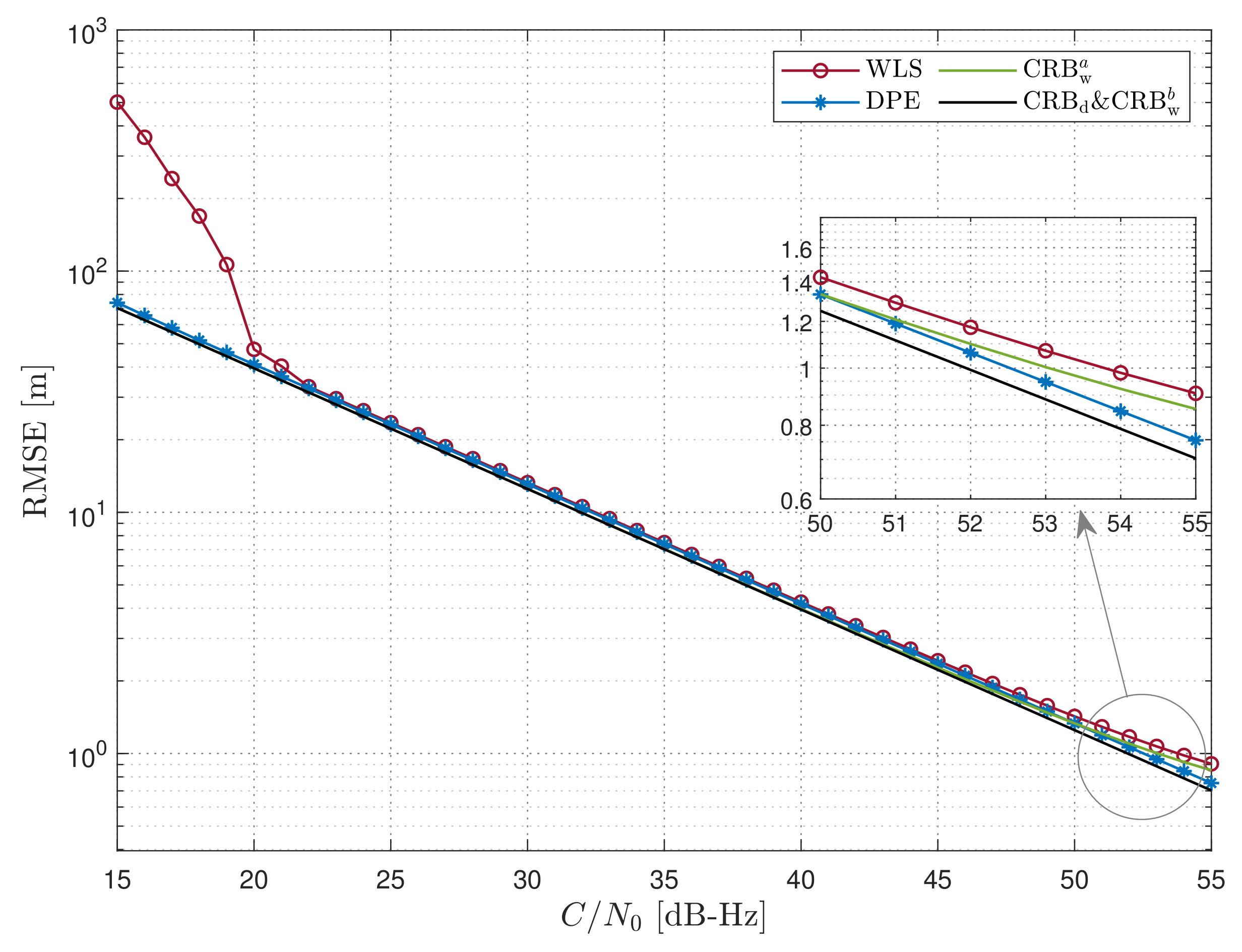
Figure 1 shows the curves plotted against the $C/N_0$ of the satellites, and all were assumed to be equal in this simulation. The blue curve, which is connected by stars, represents the RMSE of the DPE, and its corresponding bound is the black curve denoted as ${\mathrm{CRB}}_{\mathrm{d}}$. The red curve, which is connected by circles, represents the RMSE of the 2SP with WLS, and its corresponding bound from Equation (28) is the green curve denoted as ${\mathrm{CRB}}_{\mathrm{w}}^a$. As a contrast, the yellow curve represents the CRB from [23] and is shown to account for the 2SP; it is denoted as ${\mathrm{CRB}}_{\mathrm{w}}^b$. Note that in this scenario, all satellites had the same $C/N_0$, and the optimal weighted matrix was the identity matrix, which implies that ${\mathrm{CRB}}_{\mathrm{w}}^b$ and ${\mathrm{CRB}}_{\mathrm{d}}$ are the same in Figure 1. Regarding the RMSEs, both estimators exhibited similar performance for $C/N_0$ values larger than 20 dB-Hz, and both approximations approached their corresponding CRBs. In the low $C/N_0$ region, between 15 to 20 dB-Hz, WLS yielded a higher RMSE. Notably, the DPE estimator demonstrated greater robustness to high-energy noise, with a break-point that was approximately 6 dB-Hz lower than that of WLS. Concerning the derived CRBs, ${\mathrm{CRB}}_{\mathrm{w}}^a$ and ${\mathrm{CRB}}_{\mathrm{w}}^b$ mostly overlapped. In this case, the transmitted noise was the main source of error, and the cross-correlation errors were low when all satellite signals had the same $C/N_0$. Although the difference between their bounds was small, a closer look at the enlarged portion of Figure 1 reveals that ${\mathrm{CRB}}_{\mathrm{w}}^a$ was slightly higher than ${\mathrm{CRB}}_{\mathrm{w}}^b$ in the high $C/N_0$ region, between 50 to 55 dB-Hz, where the power of cross-correlation errors could reach a magnitude comparable to that of the noise. In comparison, the ${\mathrm{CRB}}_{\mathrm{w}}^a$ proposed in this study aligned more consistently with the RMSE of WLS.

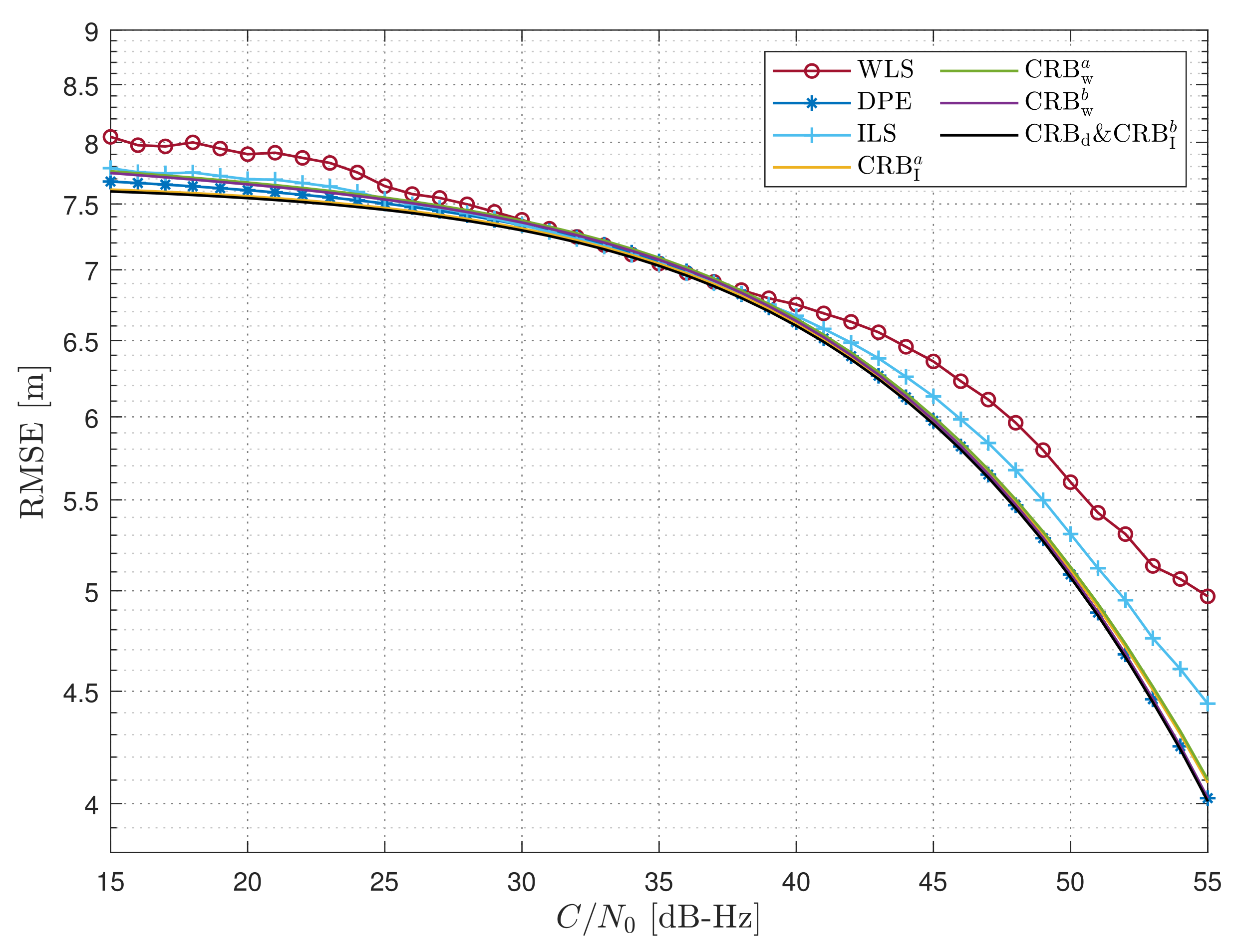
To assess the performance with varying received signal energies, we considered a scenario where all satellites, except one, had the same $C/N_0$ at 30 dB-Hz, while one varying satellite altered its $C/N_0$ value. The RMSE was calculated by averaging different satellites, treating each satellite as a varying one to eliminate the impact of geometry. Following the configuration of the curves in Figure 1, we considered another estimator, the ideal least square (ILS), an unrealistic estimator in which the true FIM is used as the weighted matrix; it is shown to account for the 2SP with the cyan curves connected by crosses. It is worth noting that the bound of the ILS, which is denoted as ${\mathrm{CRB}}_{\mathrm{I}}^b$ in [23], is the same bound as that of ${\mathrm{CRB}}_{\mathrm{d}}$ in the DPE. The bounds on the estimators and their corresponding RMSEs are presented in Figure 2. In terms of the RMSE, in the $C/N_0$ region between 25 and 55 dB-Hz, it is observed that the DPE and ILS exhibited similar performance, outperforming the WLS. The WLS achieved comparable performance to that of the other methods only when the varying satellite had a $C/N_0$ value of 35 dB-Hz. For this specific $C/N_0$, all satellites had the same energy; the appropriately weighted matrix was the identity matrix, and in this case, the WLS and ILS were equivalent, and all estimators could reach their respective bounds. In the low $C/N_0$ region, between 15 to 20 dB-Hz, both the WLS and ILS experienced a slight performance degradation. This degradation was attributed to the interference from other satellites affecting the signals of the varying satellite. Similarly, when the $C/N_0$ of the varying satellite exceeded 50 dB-Hz, the varying satellite introduced interference to the rest, leading to significant performance degradation in both the WLS and ILS. The variance of cross-correlation errors, which was related to the energies of the received signals, had a more pronounced impact in the region with a large $C/N_0$ gap. Both of these performance degradations were reflected in ${\mathrm{CRB}}_{\mathrm{w}}^a$, but not in ${\mathrm{CRB}}_{\mathrm{w}}^b$ and ${\mathrm{CRB}}_{\mathrm{I}}^b$. On the contrary, the DPE provides an optimal approach where the effects of cross-correlation errors have already been taken into account. As a result, optimal performance is achieved, approaching the CRB in all ranges of $C/N_0$.

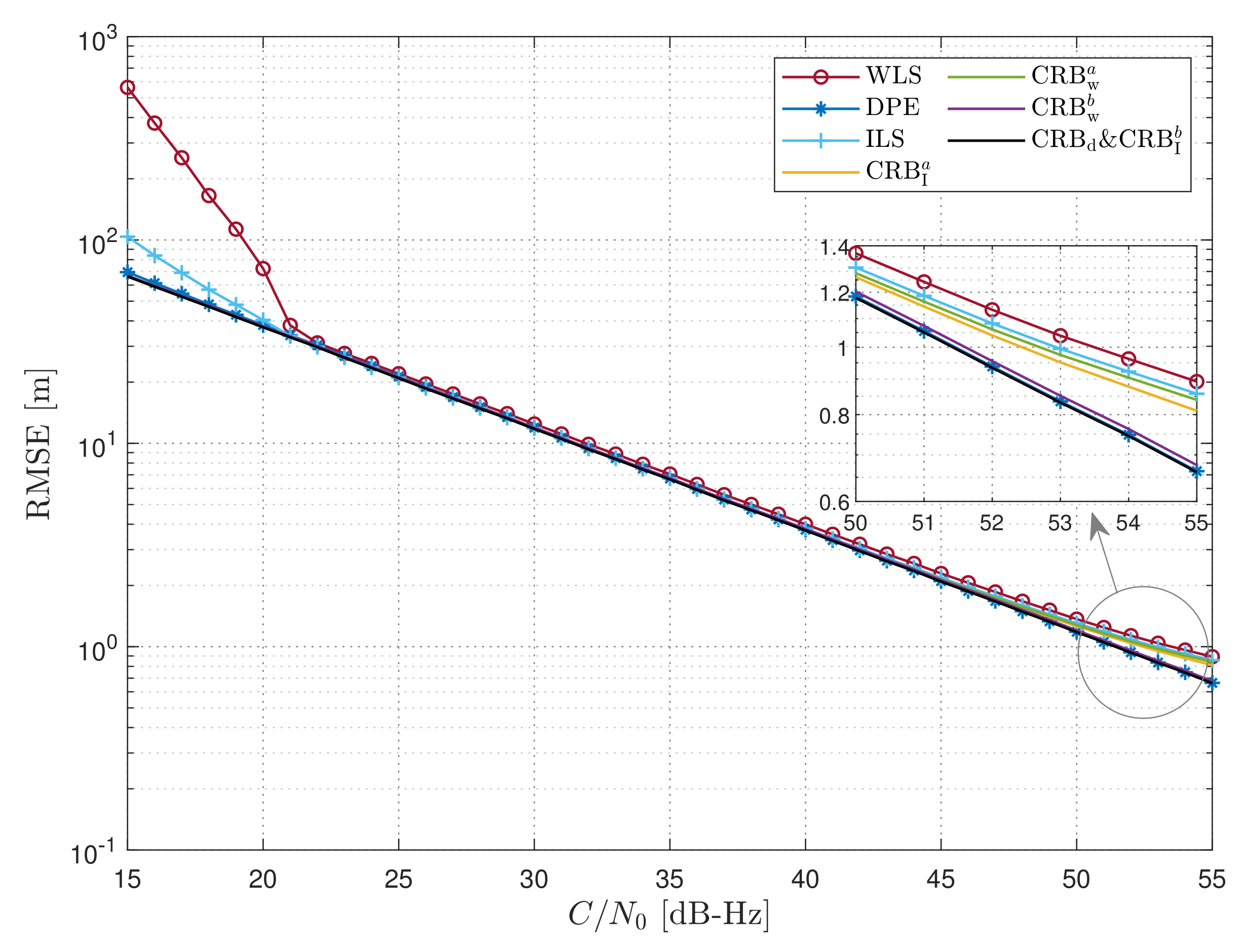
Although the signal energies of the satellites are not the same as those in Figure 2, this scenario is still considered ideal, and various approaches can be employed to eliminate individual anomalous observations, ensuring that the estimation accuracy is not significantly degraded. Comparing Figure 2 with the results in [23], the degradation of one satellite does not significantly affect the overall results. To further validate this concept, a more challenging scenario was tested. The received energy was described by a log-normal distribution, which is typically applied to land mobile channels [44]; the $C/N_0$ value of the satellites was configured to follow a normal distribution with a variable mean and a variance of 3. The bounds on the estimators and the corresponding RMSEs are presented in Figure 3. In terms of RMSEs, the WLS exhibited the most significant performance degradation, while the ILS, despite experiencing a smaller degradation, failed to match the ${\mathrm{CRB}}_{\mathrm{I}}^b$, as presented in Figure 1 and Figure 2. The RMSE of the ILS suggests that the estimation error cannot be reduced even with an optimal weighted matrix provided for the 2SP. On the other hand, the DPE demonstrated the best performance, maintaining a flat trajectory close to the CRB in all $C/N_0$ ranges. Concerning the CRBs, ${\mathrm{CRB}}_{\mathrm{w}}^b$ and ${\mathrm{CRB}}_{\mathrm{I}}^b$ did not account for the deterioration caused by the cross-correlation errors, thus failing to accurately represent the performance bounds. These bounds were lower than ${\mathrm{CRB}}_{\mathrm{w}}^a$ and ${\mathrm{CRB}}_{\mathrm{I}}^a$, even though the WLS and ILS were not achievable. In contrast, ${\mathrm{CRB}}_{\mathrm{w}}^a$ and ${\mathrm{CRB}}_{\mathrm{I}}^a$ more accurately represented the performance boundaries of the WLS and ILS, especially in the high $C/N_0$ region.

6. Discussion

Previous studies on the asymptotic performance of the 2SP can be seen as simplifying the joint time delay and Doppler shift estimation problem in GNSSs through the EXIP, which relaxes the constraints on the structure of the synchronization parameter vector; then, by using a diagonal weighted matrix to determine the confidence of these intermediate estimates, the performance of the approximate initial model is achieved by refining them through WLS minimization. As shown by the curves of the WLS in Figure 1, this allows the approximation of the CRB in certain $C/N_0$ intervals. The improvement can be illustrated from the point of view of information theory; the 2SP discards all but the most likely code phases and associated signal-to-noise ratios after the acquisition stage and then performs positioning [45]. In contrast, the DPE uses all of the information of the signal for positioning. This allows the DPE to find the best solution only from the space of possible states, so the erroneous peaks in the correlation function will most likely never be aligned, which improves the noise resistance [46]. Specifically, the 2SP can achieve the same asymptotic performance as that of the DPE when the weighted matrix is equal to the FIM of the time delay and Doppler shift [22], as shown by the curves of the ILS in Figure 2. Consequently, these studies converge on the same conclusion: the 2SP can achieve equivalent asymptotic performance to that of the DPE when an appropriately weighted matrix is employed [23,25]. However, these conclusions are derived under the condition that the estimation of the synchronization parameter in the first step is unbiased and asymptotically effective. In a GNSS, the cross-correlation error is non-negligible and is correlated with the synchronization parameters of other satellites, which leads to a bias in the synchronization parameters obtained from the first step of the individual estimation with the 2SP.

This study focuses on analyzing the asymptotic performance of the 2SP compared to that of the DPE while taking the effect of cross-correlation errors into account. Specifically, it fills the analysis of the first step for the 2SP, which has been previously overlooked. Theoretically, the difference in asymptotic performance can be obtained by comparing different optimization problems, as shown in Equations (8) and (27). It is evident that the 2SP solves the synchronization parameters by maximizing the norms of $\mathbf{y}$ and $\mathbf{D}\left(\mathit{\gamma }\right)$. This represents a special case of the DPE where the multiplication $\mathbf{D}\left(\mathit{\gamma }\right){\mathbf{D}}^{\top }\left(\mathit{\gamma }\right)$ is approximated as a diagonal matrix. However, the pseudo-orthogonality of PRN codes causes the off-diagonal elements of the multiplication $\mathbf{D}\left(\mathit{\gamma }\right){\mathbf{D}}^{\top }\left(\mathit{\gamma }\right)$ to represent non-zero cross-correlations, making it a non-diagonal matrix. In this case, a simple scaled diagonal weighing matrix does not suffice [47]. In contrast, the DPE performs an ML estimation of the PTV state, which is calculated from all visible satellites’ signals, with the aim of maximizing the norm of the projection of signal $\mathbf{y}$ onto the column space of matrix $\mathbf{D}\left(\mathit{\gamma }\right)$. The projection matrix plays the role of correcting for cross-correlation interference; then, the corrected received signals have the maximum effective projection in the signal structure matrix, thus eliminating the cross-correlation errors. Therefore, a scenario with a larger number of visible satellites with varying signal energies is provided, and the simulation results demonstrate that the cross-correlation errors cause an additional RMSE, which is even more pronounced in the high $C/N_0$ region. The simulation experiments validate that the joint processing of satellites can bring mitigation capabilities to the DPE. Although many researchers have explored how to eliminate and predict the cross-correlation errors of signals [48], receivers need access to a number of parameters in order to fully predict the cross-correlation [40]. The DPE provides a perfect opposite direction of thinking that fundamentally solves the cross-correlation errors. Although real GNSS scenarios may not have such a large difference in the $C/N_0$ values between the signals, the cross-correlation is inherently constrained by the relative Doppler shift. This study is relevant for future GNSS positioning accuracy studies, such as those of ground-based augmentation systems [49], pseudolite positioning systems [50], or passive localization based on low-Earth-orbit satellites [51]. Nonetheless, this study still holds potential for further development. One potential avenue for further development involves incorporating the spatial geometry of the satellites to improve the modeling of cross-correlation errors. Additionally, considering that cross-correlation errors are often associated with multipath errors, extending the bounds to multipath channels presents a valuable direction. Future research will focus on these issues.

7. Conclusions

This study presents a comprehensive analysis of the asymptotic performance of the 2SP and DPE while considering cross-correlation errors. The results show that the pseudo-orthogonality of PRN codes leads to a degradation in the pdf of each synchronization parameter for the 2SP. Consequently, the initial estimate of the synchronization parameter in the 2SP is not the ML. Quantitative results are presented to evaluate the performance enhancements achieved by the DPE when treating cross-correlation errors as AWGN. Theoretical expressions for the estimated variances of both approaches are derived, providing a more strict result that shows that the 2SP is not asymptotically efficient, and the DPE consistently outperforms the 2SP in GNSSs. Simulation tests further validate the superior performance of the DPE, highlighting its ability to resist cross-correlation errors through the joint processing of satellite signals. This key feature positions the DPE as a robust solution that is capable of addressing challenges related to multi-access interference and near–far effects.