A Wide-Angle Hyperspectral Top-of-Atmosphere Reflectance Model for the Libyan Desert

Abstract

Reference targets with stability, uniformity, and known reflectance on the Earth’s surface, such as deserts, can be used for the absolute radiometric calibration of satellite sensors. A wide-angle hyperspectral reflectance model at the top of atmosphere (TOA) over such a reference target will expand the applicability of on-orbit calibration to different spectral bands and angles. To achieve the long-term, continuous, and high-precision absolute radiometric calibration of remote sensors, a wide-angle hyperspectral TOA reflectance model of the Libyan Desert was constructed based on spectral reflectance data, satellite overpass parameters, and atmospheric parameters from the Terra/Aqua and Earth Observation-1 (EO-1) satellites between 2003 and 2012. By means of angle fitting, viewing angle grouping, and spectral extension, the model is applicable for absolute radiometric calibration of the visible to short-wave infrared (SWIR) bands for sensors within viewing zenith angles of 65 degrees. To validate the accuracy and precision of the model, a total of 3120 long-term validations of model accuracy and 949 cross-validations with the Landsat 8 Operational Land Imager (OLI) and Suomi National Polar-Orbiting Partnership (NPP) Visible Infrared Imaging Radiometer Suite (VIIRS) satellite sensors between 2013 and 2020 were conducted. The results show that the TOA reflectance calculated by the model had a standard deviation (SD) of relative differences below 1.9% and a root-mean-square error (RMSE) below 0.8% when compared with observations from the Moderate Resolution Imaging Spectroradiometer (MODIS) and Landsat 8 OLI. The SD of the relative differences and the RMSE were within 2.7% when predicting VIIRS data.

1. Introduction

High temporal radiometric calibration updates enable the long-term monitoring and correction of the on-orbit degradation of a remote sensor’s radiometric response characteristics. This ensures the continuity and consistency of long-term observation data, which are crucial for observing long-term climate and environmental changes and for the fusion of multisensor remote sensing data [1,2,3,4,5].

Commonly used on-orbit calibration methods include stable target field tracking and cross-calibration [6,7]. Earth-based invariant targets, ground sites, and targets actively monitored by aircraft utilize satellite products from ground pseudo-invariant calibration sites (PICSs) to achieve long-term tracking calibration. However, its accuracy is limited by the accuracy of the surface reflectance retrieved from remote sensing data and atmospheric parameters, such as the aerosol optical depth (AOD), water vapor, and ozone, as well as the asynchrony of satellite product acquisition times. To further improve the calibration accuracy, cross-calibration methods can be employed. Cross-calibration uses a sensor with recognized high accuracy and stability as a reference to perform a degradation correction of the sensor to be calibrated through matching in terms of the location, time, spectrum, and angle. Cross-calibration is advantageous in eliminating atmospheric effects. However, strict adherence to the cross-calibration conditions can limit the calibration frequency of the sensor. It is also challenging to find an Earth observation sensor with sufficient long-term stability that meets the requirements for monitoring climate and environmental changes over decades. In addition, alternative means, such as aircraft, can be used for cross-calibration; such means offer better synchronization but at higher costs and with challenges in operationalization [8,9].

In recent years, to increase the calibration frequency while effectively managing the budget, researchers have proposed on-orbit calibration methods using an absolute radiometric calibration model based on ground PICSs. Helder et al. [10] discussed how to use PICSs for the absolute radiometric calibration of Landsat satellites. He established a simple empirical model for the solar zenith angle (SZA) based on years of accumulated data from Terra MODIS by considering only nadir-looking view angles within ±7.5° in the Libyan Desert. The model predicted the TOA reflectance for selected bands of Landsat 7 and used gain factors to correct for spectral differences between the two sensors. The comparison between the model calculations and actual measurements from Landsat 7 showed an accuracy within 6% and a precision within 3%, demonstrating the feasibility of using PICSs for absolute calibration. Mishra et al. [11] further expanded on Helder’s work and made improvements by introducing the viewing zenith angle (VZA) into the model by considering atmospheric effects and performing atmospheric corrections, which was applicable to moderate-resolution sensors with viewing angles of up to 20°. Comparisons between the improved model’s predictions and satellite observations from Landsat 7 ETM+, Aqua MODIS, MERIS, Landsat 8 OLI, and UK-2 DMC indicated an accuracy of 3% and a precision of 2%. Raut et al. [12] extended the model to five PICSs in the Sahara Desert and achieved accuracy and precision comparable with those of the Libyan Desert model. However, existing models restrict the viewing angle to within 20° during calibration, making them challenging to apply to sensors with larger viewing angles.

For the spectral differences between different sensors, Helder et al. utilized Hyperion to extend the applicable bands of a model. He strictly matched five pairs of MODIS/Hyperion images with VZAs within ±5° and an observation time difference of less than 30 min. The scaling factors for each band were calculated and averaged to obtain corresponding gain factors. However, the calculation of the gain factors was constrained by strict spatiotemporal matching, and the number of image pairs was limited.

To enhance the model applicability and performance, this study established a wide-angle hyperspectral TOA reflectance model for the Libyan Desert. Based on the stable characteristics of stable targets, both on the surface and in the atmosphere, a TOA reflectance model for the Libyan Desert was fitted using long-term multisatellite TOA data. By inputting the SZA, solar azimuth angle (SAA), VZA, viewing azimuth angle (VAA), and atmospheric parameters, the TOA reflectance results could be calculated. This model is suitable for absolute radiometric calibration of the visible to SWIR bands within VZAs up to 65°. The accuracy and applicability of the model were validated by comparing the model results with Landsat and VIIRS observations.

The remainder of this article is organized as follows. Section 2 describes the preparatory work for modeling, including the study site and the sources of satellite image data. It also presents the data quality control methods and analyzes the sensitivity of TOA reflectance to atmospheric parameters. Section 3 explains how the multiband TOA reflectance model was established and extended to a hyperspectral resolution, along with performance evaluation methods. Section 4 presents validation of the long-term accuracy of the model using MODIS data and presents a cross-validation performed using Landsat 8 OLI and Suomi NPP VIIRS data. Section 5 provides a summary and discusses the broader feasibility of the model.

2. Data Collection and Analysis

2.1. PICSs Overview

The Committee on Earth Observation Satellites (CEOS) recommends six PICSs for the long-term on-orbit radiometric calibration of Earth observation optical sensors. These sites possess several favorable characteristics, including temporal stability, spatial uniformity, and homogeneity [13,14].

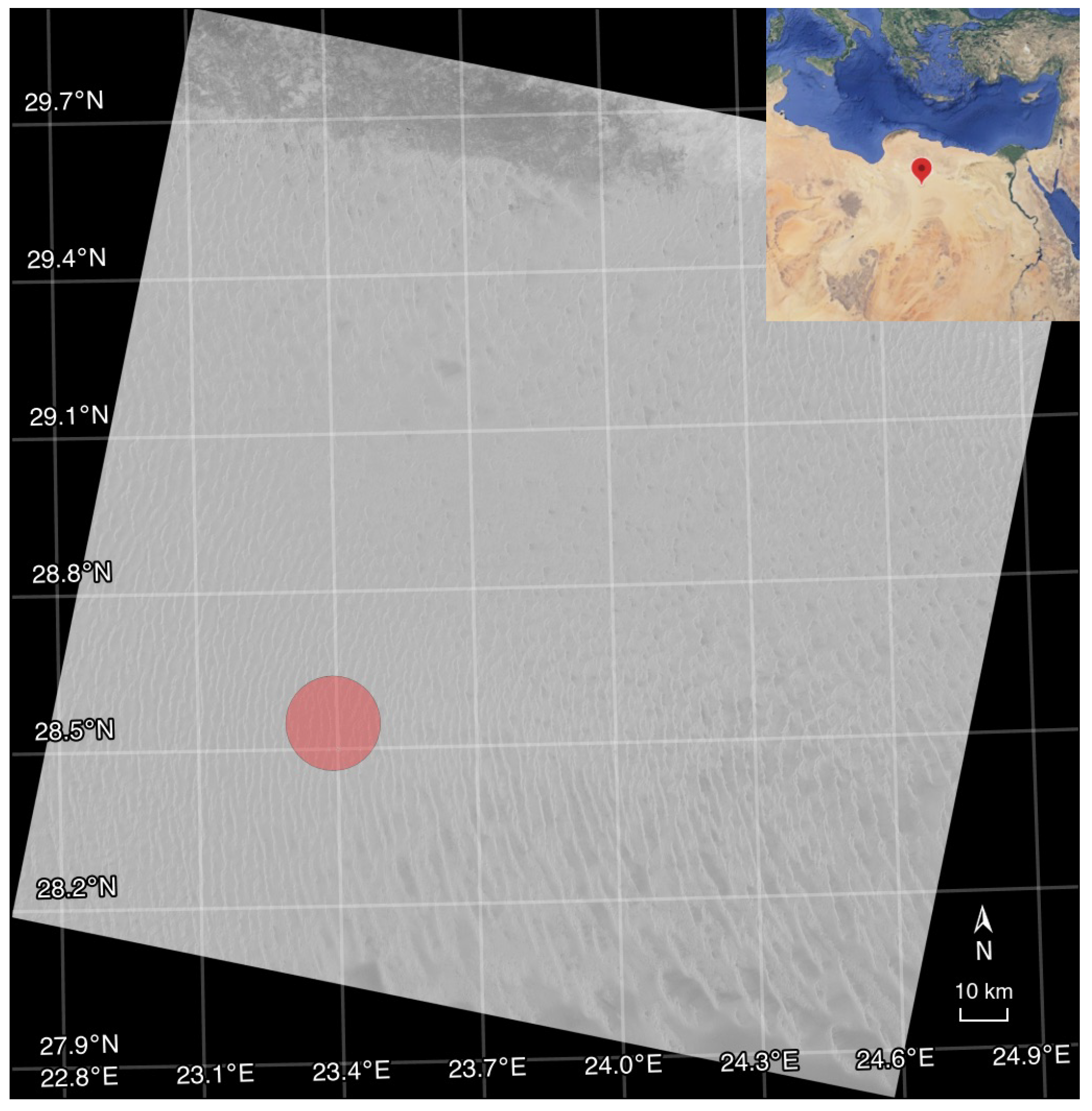
One of these PICSs is Libya 4, which is located in the Libyan Desert, with consistently high reflectance throughout the year. Libya 4 is widely recognized as one of the most stable PICSs and has been extensively utilized [11,15]. Following CEOS recommendations, this study considered a circular area with a center at coordinates (28.55°N, 23.39°E) and a diameter of 20 km [13]. Figure 1 is an image generated using the near-infrared (NIR) band (865 nm) of Landsat 8’s TOA reflectance that was captured on 20 August 2018. The region of interest is highlighted in red.

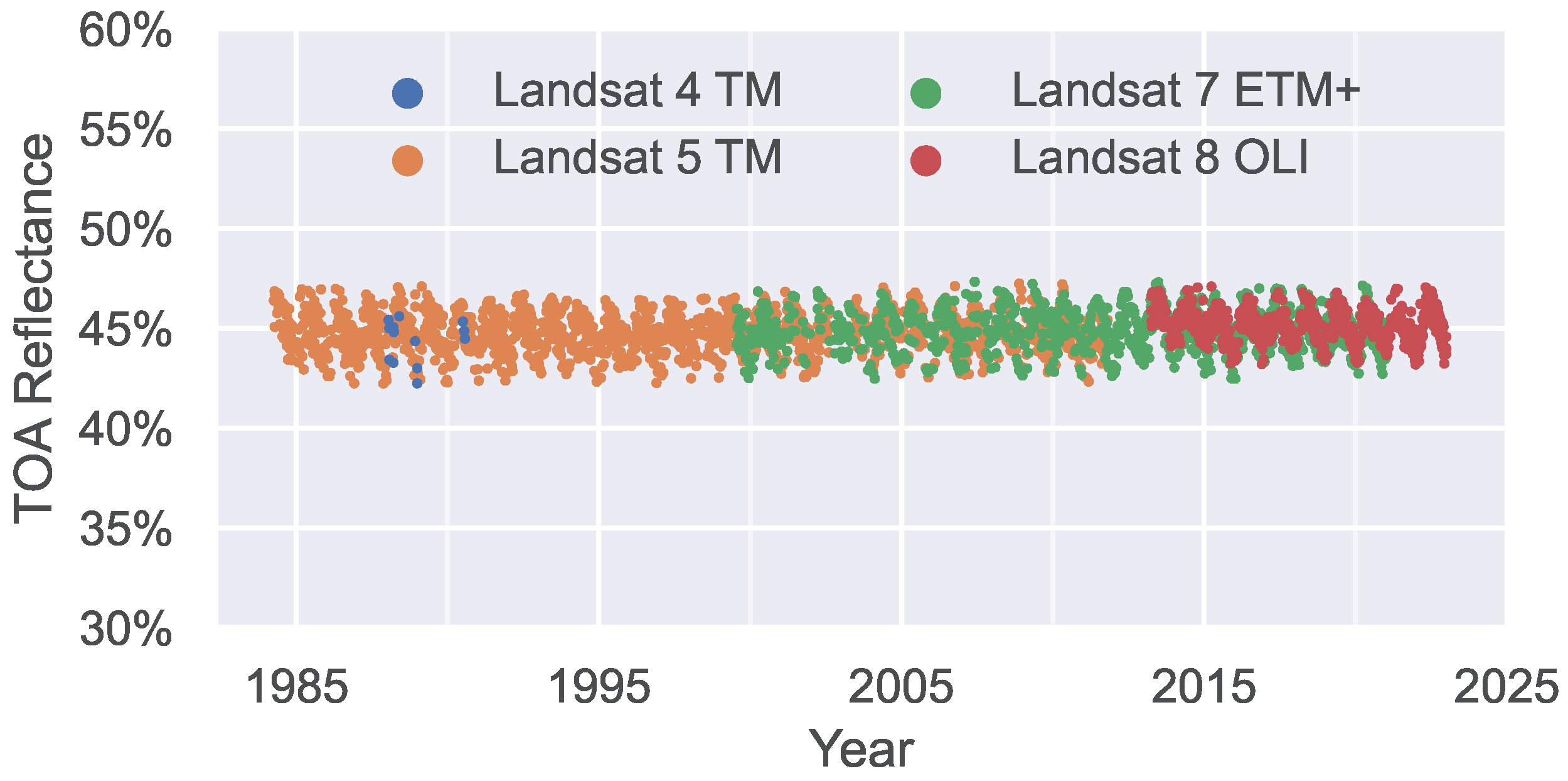
Figure 2 shows the stability of the TOA reflectance in the Libyan Desert from 1985 to 2021. The TOA reflectance data in the red band are extracted from the Landsat series of satellites. There are minor variations in the relative spectral response profiles among corresponding bands from different Landsat sensors [16]. The data from Landsats 4, 5, and 7 were spectrally adjusted to match Landsat 8 OLI band 4 [17]. The TOA reflectance does not exhibit any significant trend.

2.2. Data Sources

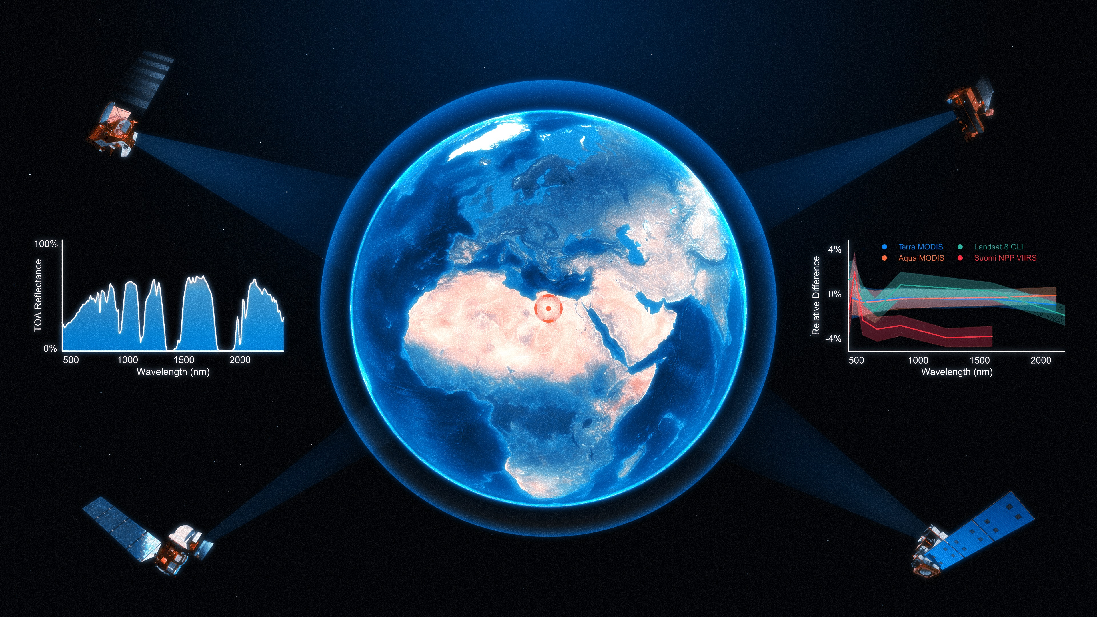
The study presented in this article relied on data from the following five satellite sensors: Terra/Aqua MODIS, Landsat 8 OLI, Suomi NPP VIIRS, and EO-1 Hyperion. The spatial resolutions and temporal ranges of the sensors used in this study are presented in

Table 1. Sensors and their spatial resolutions and temporal ranges used in this study.

Satellite	Sensor	Spatial Resolution (m)	Temporal Range
Terra	MODIS	250/500	2003–2020
Aqua	MODIS	250/500	2003–2020
Landsat 8	OLI	30	2013–2020
Suomi NPP	VIIRS	750	2013–2020
EO-1	Hyperion	30	2008–2017

.

MODIS is a remote sensing sensor developed by NASA for studying the Earth’s atmospheric system. This study used MODIS data from the Terra (morning overpass) and Aqua (afternoon overpass) satellites, which image the entire Earth every one to two days [18,19].

MODIS has a radiometric resolution of 12 bits and offers up to 36 spectral bands [20,21]. The data used in this study for establishing the TOA reflectance model are derived from the first seven bands, covering the visible to SWIR region. The spatial resolution of these bands is either 250 m (bands 1 and 2) or 500 m (bands 3–7), as shown in

Table 2. Spectral bands of Terra/Aqua MODIS.

Band	Start (nm)	End (nm)	Center (nm)
1	620	670	659
2	841	876	865
3	459	479	470
4	545	565	555
5	1230	1250	1240
6	1628	1652	1640
7	2105	2155	2130

.

The MODIS data products used in this study include version 6.1 of MOD021KM, MYD021KM, and MYD08_D3. These products resample the data from bands 1 to 7 to a spatial resolution of 1000 m. MOD021KM/MYD021KM provides level 1B TOA radiance, reflectance, and related parameters [22,23]. MYD08_D3 provides daily atmospheric data, including AOD, water vapor, and ozone, which are used for atmospheric correction of the TOA reflectance model [24].

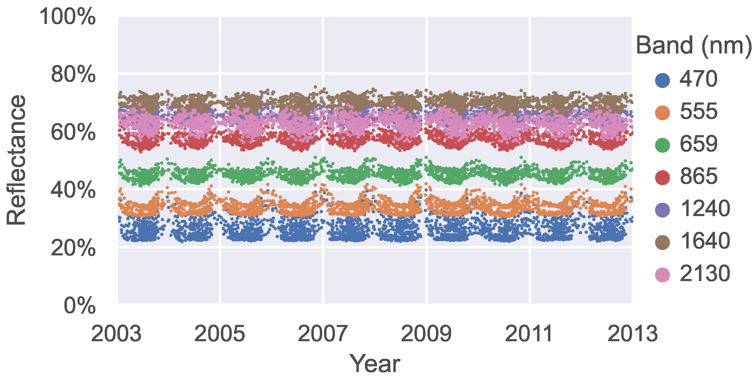
Figure 3 illustrates the long-term TOA reflectance for bands 1 to 7 of Aqua MODIS over the Libyan Desert from 2003 to 2012. The TOA reflectance remained stable over time for each band.

Landsat 8 was launched in 2013 and is currently operated by the United States Geological Survey (USGS). It carries the OLI instrument, which has a swath width of 185 km and a length of 180 km, with a ground resolution of 30 m [25]. This study focused on the first seven spectral bands for validation, covering wavelengths from visible to SWIR, as shown in

Table 3. Spectral bands of Landsat 8 OLI.

Band	Start (nm)	End (nm)	Center (nm)
1	434.97	450.95	442.96
2	452.02	512.06	482.04
3	532.74	590.07	561.41
4	635.85	673.32	654.59
5	850.54	878.79	864.67
6	1566.50	1651.22	1608.86
7	2107.40	2294.06	2200.73
8	503.30	675.70	589.50
9	1363.24	1383.63	1373.43

.

Suomi NPP is a low-Earth-orbit meteorological satellite that was launched in 2011. One of the key instruments on board Suomi NPP is VIIRS, which is a cross-track scanning radiometer. It provides twice-daily global coverage of the Earth’s surface and collects imagery data at a moderate spatial resolution of 750 m. VIIRS has 22 spectral bands, covering the wavelength range from 0.4 to 11.8 mm [26]. The VIIRS data are from NASA’s ArchiveSet 5200. This article studies the moderate-resolution bands in the visible and NIR region of VIIRS, as shown in

Table 4. Moderate-resolution spectral bands of Suomi NPP VIIRS.

Band	Start (nm)	End (nm)	Center (nm)
1	402	422	415
2	436	454	445
3	478	498	490
4	545	565	555
5	662	682	673
6	739	754	746
7	846	885	865
8	1230	1250	1240
9	1371	1386	1378
10	1580	1640	1610
11	2225	2275	2250

.

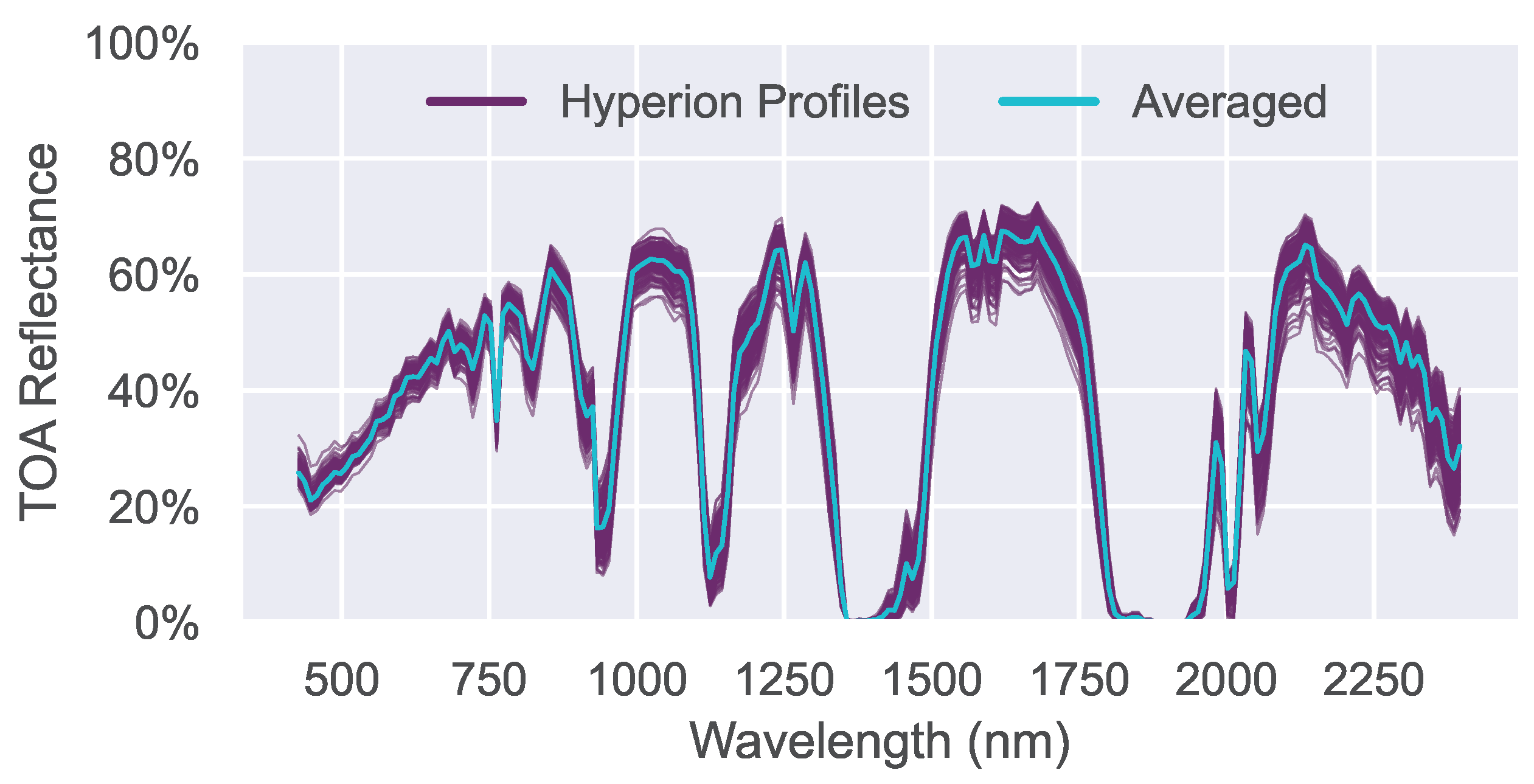
EO-1 was launched in 2000. Hyperion is one of the primary instruments on board and the first space-based high-resolution hyperspectral imaging instrument. It provides 198 calibrated spectral bands, including visible to NIR bands (8–57) and SWIR bands (77–224), covering wavelengths from 430 to 2400 nm. The sampling interval is approximately 10 nm. In this article, Hyperion data were used to provide spectral reflectance profiles [27].

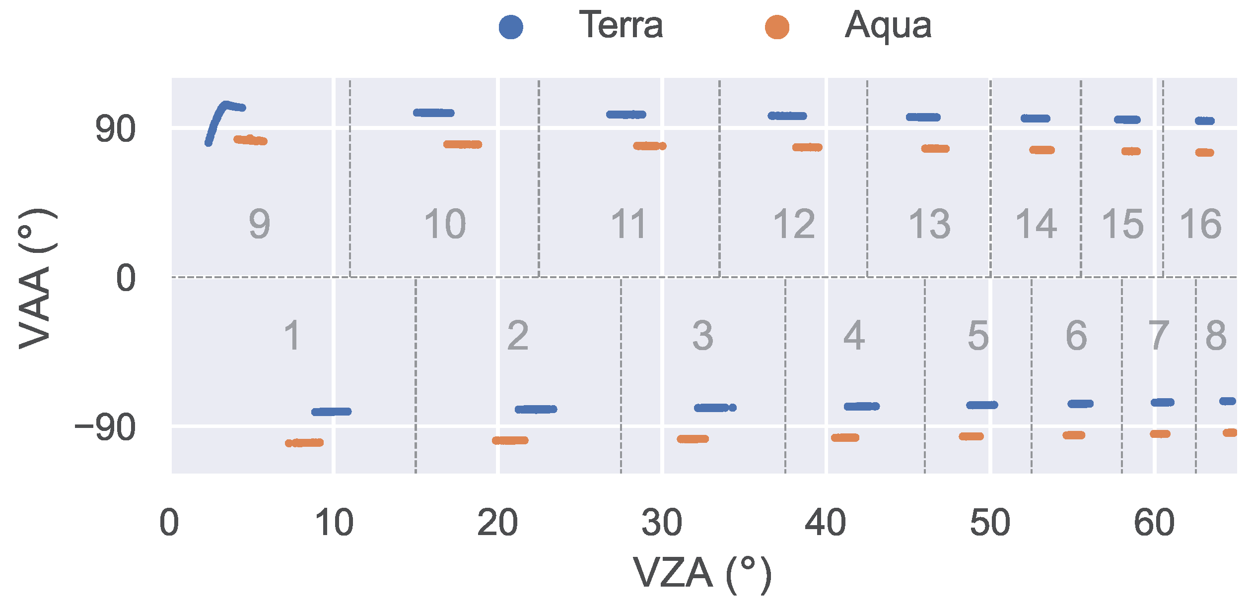
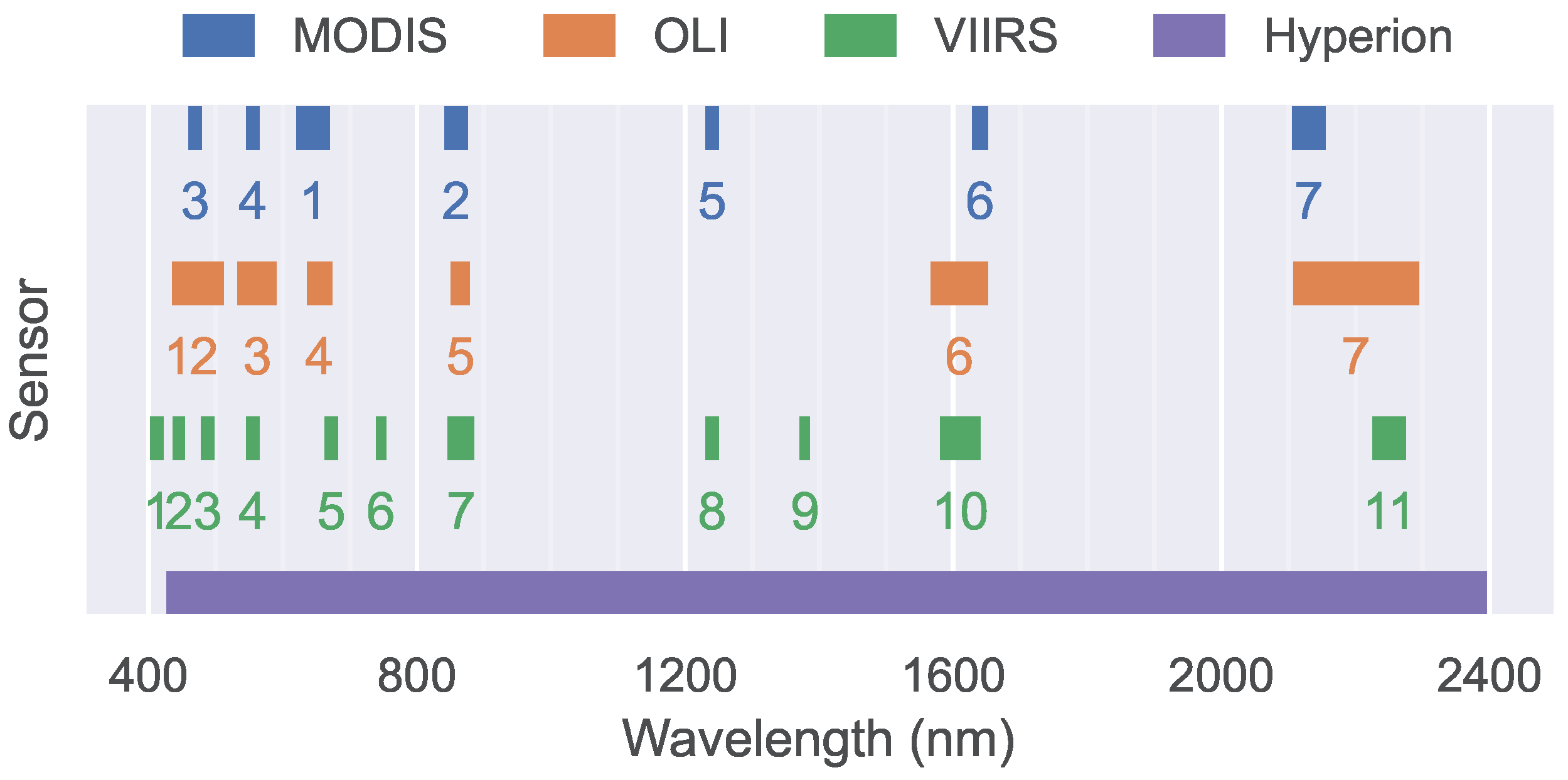
MODIS images have a large coverage area, high temporal resolution, and the longest operational period among all mentioned satellites, making more angle inputs available for the TOA reflectance model. Figure 4 shows the band coverage of the four sensors. Differently colored lines represent different sensor bands, with the numbers below indicating their respective band numbers.

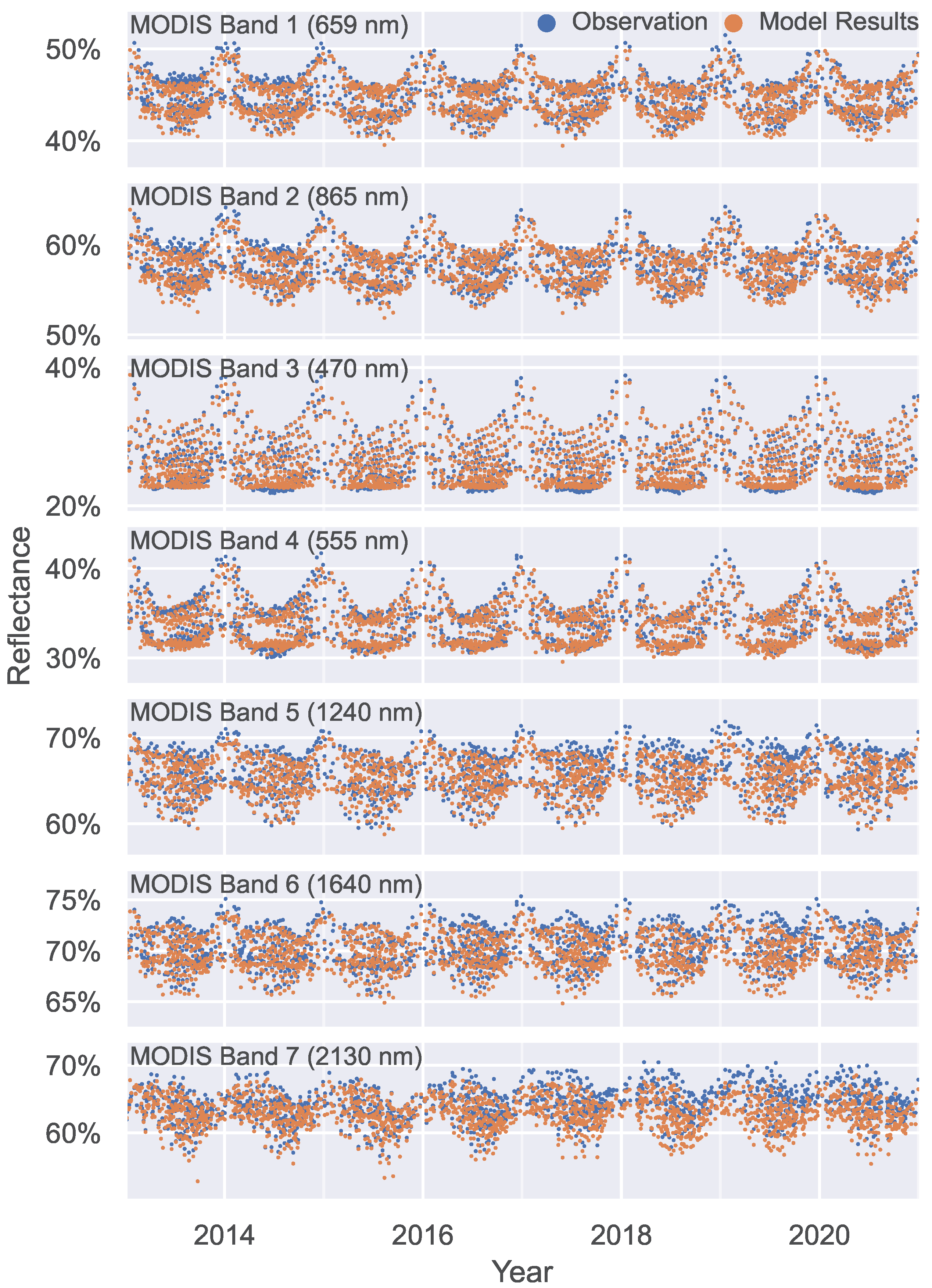
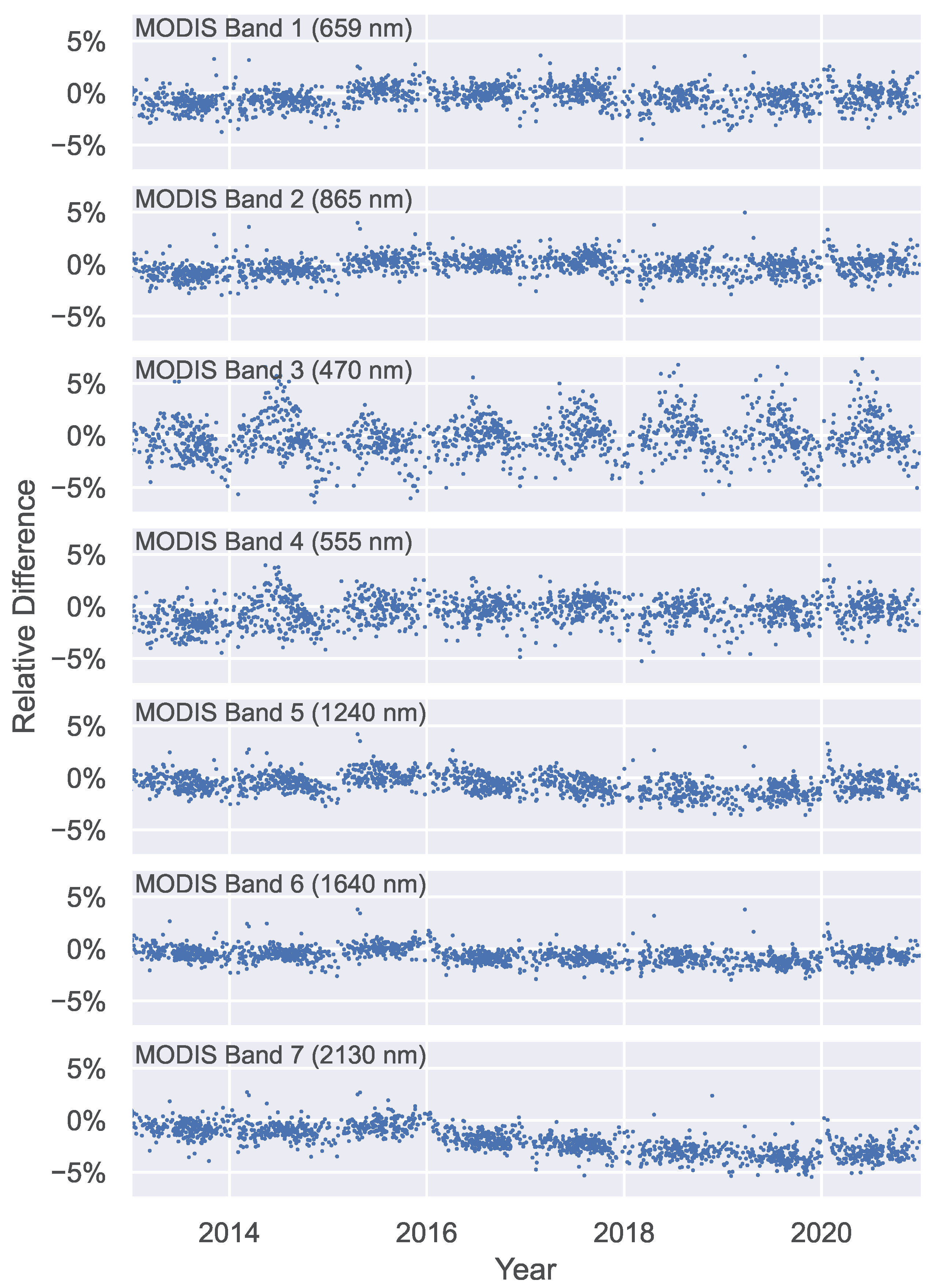
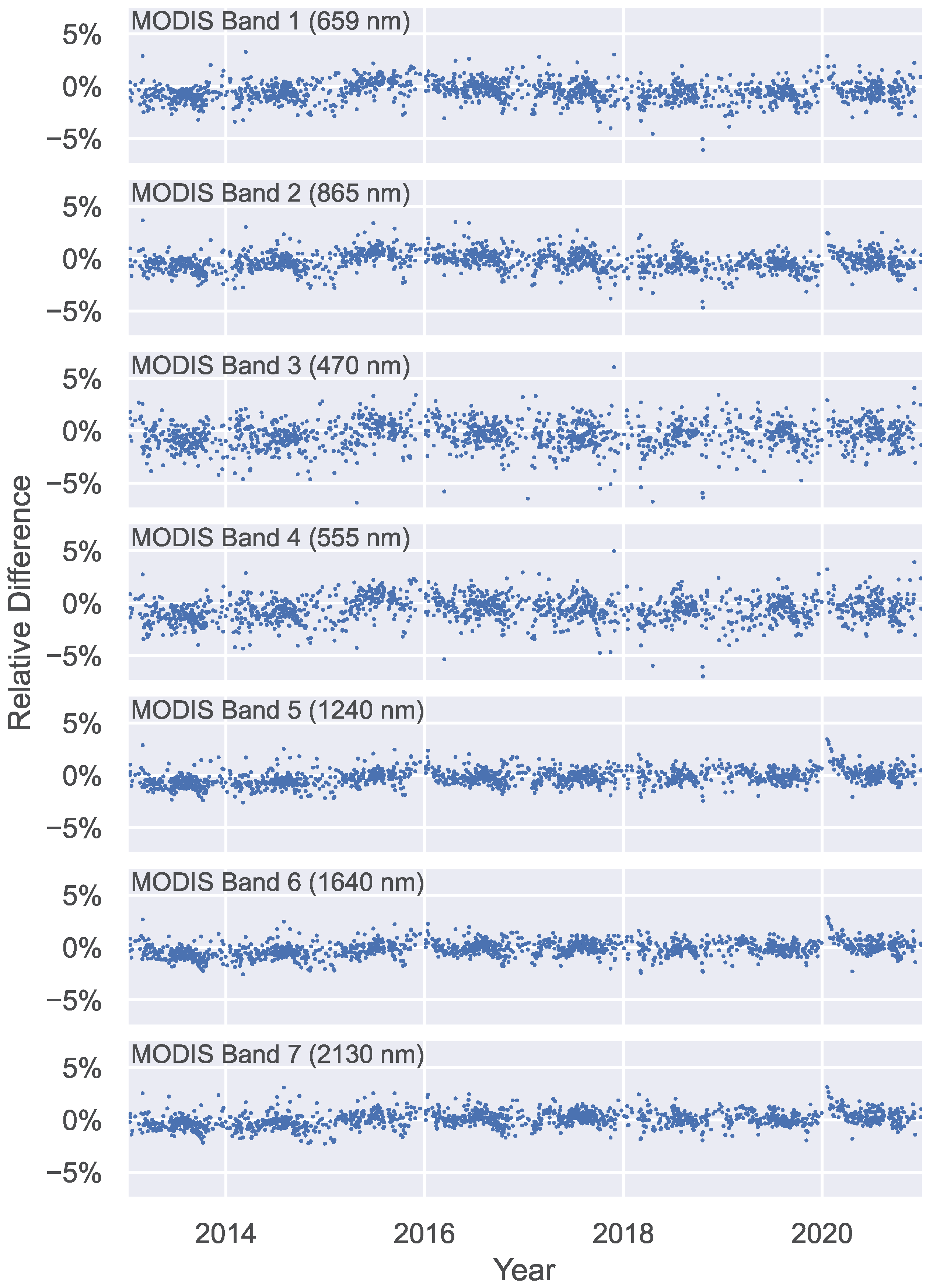
Over 7000 Level 1B MODIS images obtained from NASA yield calculated TOA reflectance data and corresponding angle data with which to fit the model parameters. After model establishment, these data were used to validate the accuracy of the long-term TOA reflectance predictions.

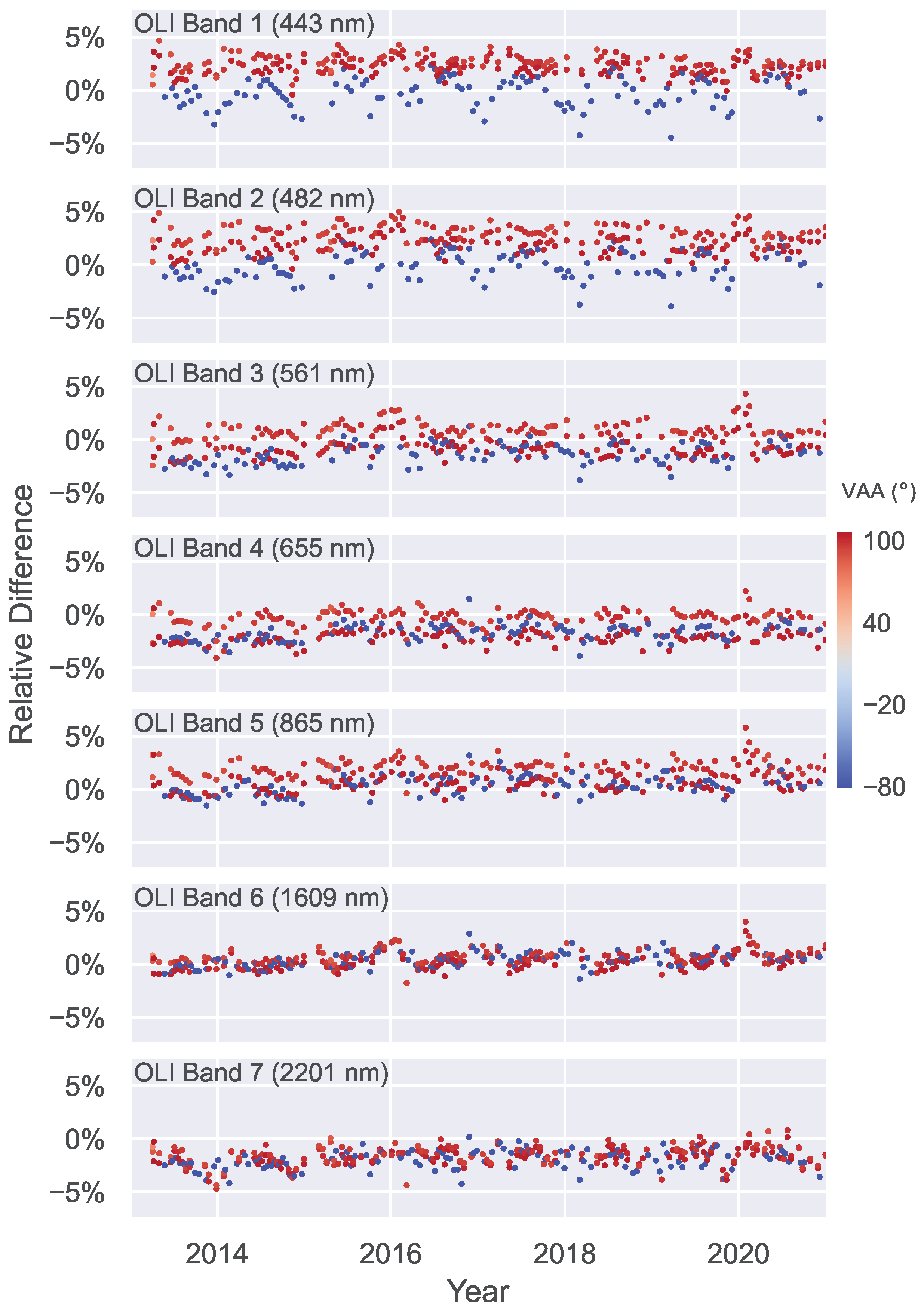
To further validate the accuracy and test the computational precision of the TOA reflectance model compared with other satellite sensors, this study used satellite data acquired from EO-1 Hyperion, Landsat 8 OLI, and Suomi NPP VIIRS. OLI’s Level 1T TOA reflectance data and Hyperion’s TOA hyperspectral radiance data are publicly available from the USGS [28,29]. The VIIRS data were obtained from NASA’s public database [30].

This study primarily used Python 3.10 during the data processing and analysis, along with several third-party libraries [31]. NumPy 1.24 and pandas 2.0 were used for fundamental computations [32,33]. Matplotlib 3.7, OpenCV 4.7, and seaborn 0.12 were used for data visualization [34,35,36]. Statsmodels 0.14 was used for modeling [37]. The acquisition of satellite images was facilitated using the requests 2.31 library. The processing of image data involved the application of pyhdf 0.10, netCDF4 1.6, and GDAL 3.8 libraries [38,39]. All of these libraries were adopted for comprehensive data analysis and presentation.

2.3. Data Quality Control

Daily TOA reflectance data were extracted from Terra/Aqua MODIS images between 2003 and 2012 and used to build the TOA reflectance model. A single image may contain cloud cover, reducing the model’s accuracy. Therefore, the data quality was assessed based on the nonuniformity of the target area. Non-clear-sky records were removed by setting a threshold for spatial nonuniformity. Any data with spatial nonuniformity higher than this threshold were considered associated with non-clear-sky weather and were ignored during the model fitting process. The spatial nonuniformity was defined as the coefficient of variation (CV) of all pixels within the target area in the image as follows:

$$\mathrm{CV}=\frac{\sigma }{\mu }.$$

(1)

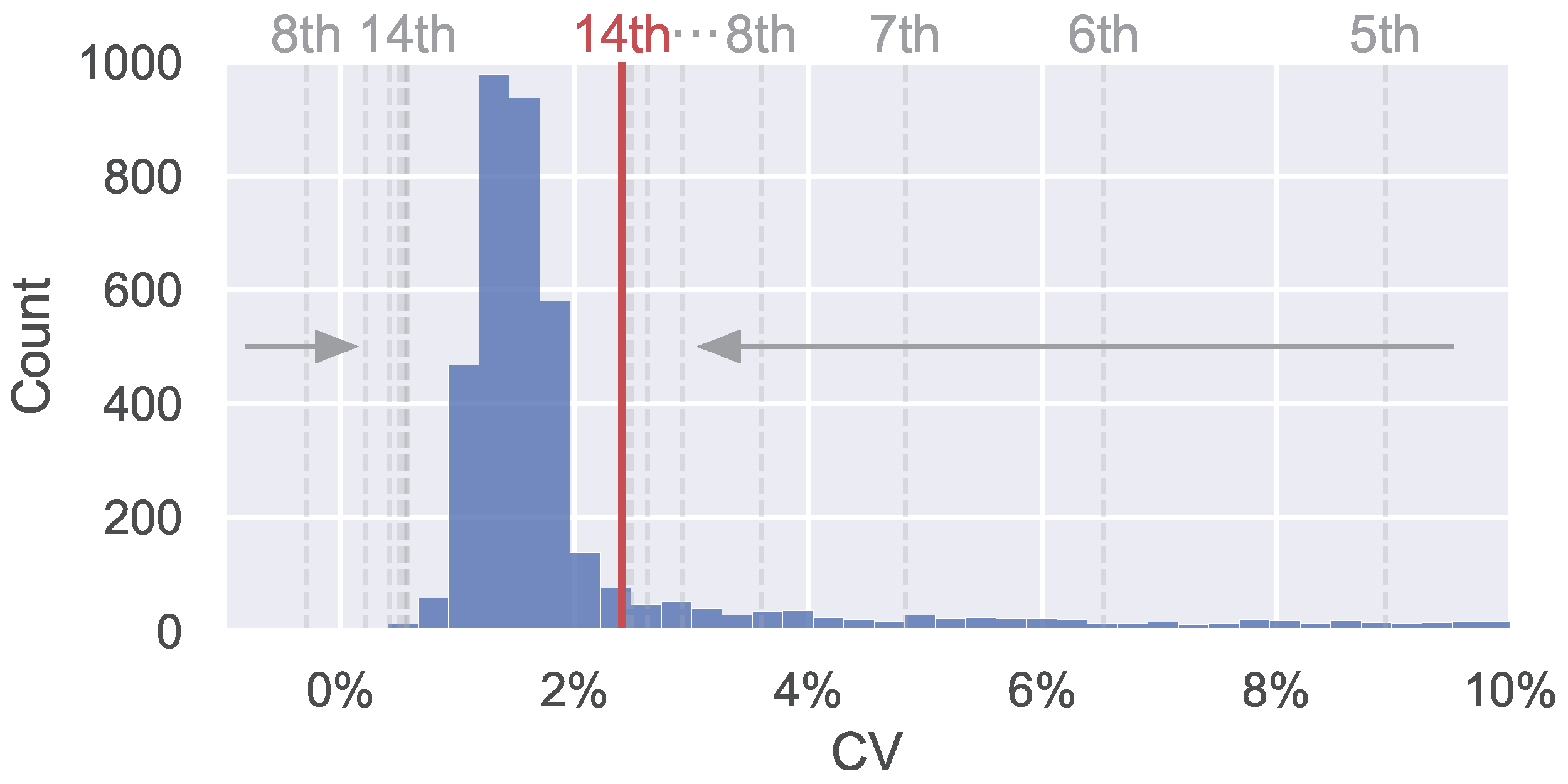
Here, $\mu$ represents the mean of all pixels within the target area in the satellite image, and $\sigma$ represents the SD. This is a normalized measure of dispersion, also known as the relative standard deviation. An abnormally large CV value indicates cloud cover in the target area, meaning that it is not applicable for radiometric calibration. By calculating the CV for the target area in all images, a histogram of the daily nonuniformity distribution for the Libyan Desert was obtained, as shown in Figure 5. The CV values roughly followed a normal distribution.

According to the $3\sigma$ rule, nearly 99.7% of the values drawn from a normal distribution fall within three SDs. Due to the sparsity of the distribution and the presence of outliers, an iterative shrinking method was used to determine the threshold for spatial nonuniformity. This method gradually narrows down the boundary of the CV distribution through iterative steps, approaching the central region of the distribution. In each iteration, $\mu$ and $\sigma$ were recalculated, and values outside the $\mu \pm 3\sigma$ interval were removed until all values fell within the interval. In the last iteration, the upper threshold limit was set to $\mu +3\sigma$. Data points with CV values exceeding this threshold were labeled “non-clear-sky” data and were not used in the modeling process.

The dashed lines in Figure 5 represent the boundaries of the $3\sigma$ intervals for each iteration. For readability, these boundaries are only partially shown. The boundaries for iterations 1–7, which were far from the peak, are not shown, and the boundaries for iterations 9–13, which were densely packed, are not labeled. By the 14th iteration, all values fell within the $3\sigma$ interval. At this point, the iteration process was terminated, and the upper limit of 2.4% represented the desired threshold for nonuniformity.

2.4. Sensitivity Analysis of Atmospheric Parameters

During the imaging process of a remote sensor, solar radiation first enters the Earth’s atmosphere from outer space and reaches the Earth’s surface [40]. It is then reflected from the surface and scattered back to the onboard sensor through the atmosphere. Solar radiation is absorbed and scattered along its transmission path by various atmospheric molecules and aerosols. Due to the influence of atmospheric absorption and scattering, the apparent surface reflectance decreases once the reflected radiation reaches the TOA [41,42].

Second Simulation of a Satellite Signal in the Solar Spectrum (6S) is a computer code that accurately simulates the above process [43,44]. In this study, the vector version of the 6S model was used to simulate atmospheric radiative transfer in the visible and NIR bands under different atmospheric conditions. By taking geometrical conditions, atmospheric conditions, spectral bands, altitude, aerosol model type, ground reflectance, and other parameters as inputs, this model can produce the apparent reflectance values at the TOA after the traversal of the atmospheric path.

Understanding the influence of the atmosphere is valuable for model development. To quantify the impact of the atmosphere on the radiometric calibration of an onboard sensor, it is necessary to evaluate the sensitivity of the sensor to AOD, water vapor, and ozone. For this purpose, this study considers data from a clear-sky day on 3 July 2019. The atmospheric parameters for that day were extracted from the Aqua MODIS atmospheric product [24], as shown in

Table 5. Atmospheric and surface parameters in the Libyan Desert on 3 July 2019.

Date	AOD	Water Vapor	Ozone
3 July 2019	0.126	1.823 cm	267.5 DU

.

The analysis was performed using a single-variable method. In each test focusing on a specific atmospheric parameter, that parameter was varied while other parameters were held constant. Multiple values were chosen for each parameter based on its distribution. The TOA reflectance was recalculated for each value using the 6S model and compared with the actual TOA reflectance value using

$$\begin{array}{c}\hfill \Delta {\rho }_{v_i}=\frac{{\rho }_{v_i}-{\rho }_{v_0}}{{\rho }_{v_0}}\end{array}$$

(2)

Here, ${\rho }_{v_0}$ is the original TOA reflectance calculated by the actual atmospheric parameters (as shown in Table 5). ${\rho }_{v_i}$ represents the reflectance result recalculated after a specific value is taken from the distribution of a single variable among AOD, water vapor, and ozone. $\Delta {\rho }_{v_i}$ is their relative difference.

After all the calculations were complete, the impacts of different atmospheric parameter variations on radiative transfer were analyzed.

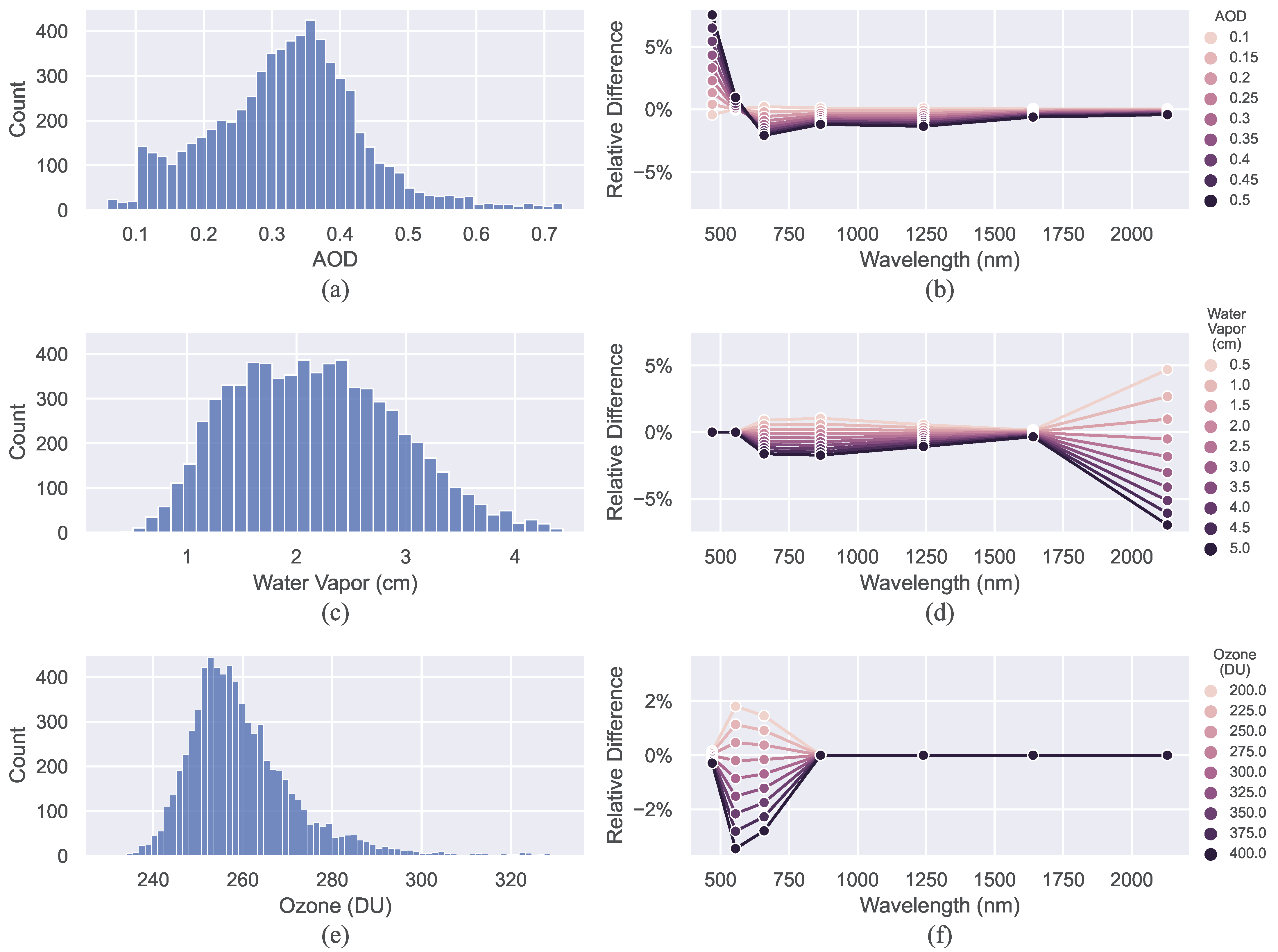
The AOD data over the Libyan Desert were extracted from MODIS MYD08_D3’s Deep_Blue_Aerosol_Optical_Depth_550_Land_Mean dataset. The AOD values were mainly between 0.1 and 0.5, as shown in Figure 6a.

Nine AOD values ranging from 0.1 to 0.5 at uniform intervals of 0.05 were selected. Figure 6b shows that in the blue (470 nm) and red (650 nm) bands, the relative difference $\Delta {\rho }_{v_i}$ varied by 8.0% as the AOD value increased from 0.1 to 0.5. The relative differences for other bands were within 2.3%.

The long-term column water vapor data were extracted from MYD08_D3’s Water_Vapor_Near_Infrared_Clear_Mean dataset. The values over the Libyan Desert ranged mainly between 0.5 and 5 cm, as shown in Figure 6c.

Ten water vapor values ranging from 0.5 to 5.0 cm were uniformly sampled at intervals of 0.5 cm. As the value increased from 0.5 to 5.0 cm, the relative difference in the 2130 nm SWIR band decreased by 11.6%, while those in the other bands remained below 2.8%, as shown in Figure 6d.

Considering the electromagnetic absorption of water vapor, it can be inferred that the 2130 nm SWIR band was influenced by atmospheric water vapor absorption. This indicates that the performance of the TOA reflectance model near 2130 nm could also be affected by water vapor [45].

The total ozone burden data were extracted from the Total_Ozone_Mean dataset in the MYD08_D3 product. The ozone values in the Libyan Desert were primarily distributed between 200 and 350 DU (Dobson unit), as shown in Figure 6e.

Nine ozone values ranging from 200 to 400 DU were uniformly sampled at intervals of 25 DU. Figure 6f shows that as the ozone increased from 200 to 400 DU, the relative differences in the green (555 nm) and red (659 nm) bands increased by 5.3% and 4.2%, respectively, indicating the influence of atmospheric ozone absorption [46]. In other bands, particularly between 865 and 2130 nm, the relative difference remained below 0.01%.

From the single-variable sensitivity analyses above, it is evident that the AOD and ozone had more significant impacts on the visible spectrum, while water vapor significantly influenced the 2130 nm SWIR band. This suggests that atmospheric parameters could affect a model’s accuracy, particularly at solid absorption wavelengths. Therefore, it was necessary to perform atmospheric correction and introduce atmospheric parameters into the TOA reflectance model.

3. Methods

3.1. Grouping by Viewing Angles

To improve the fit performance of the TOA reflectance model, the relationships between the TOA reflectance and solar/viewing angles were investigated using corresponding data collected from over 7000 Aqua MODIS images. Taking the blue band (470 nm) as an example, the data revealed a positive correlation between the TOA reflectance and SZA, as shown in Figure 7.

In Figure 7, the dots are plotted with different colors based on their VAA values. The azimuth is defined as a horizontal angle measured clockwise from north. The TOA reflectance exhibited significant variations for different VZA and VAA values. Therefore, grouping the data based on the viewing angles enhanced the fit performance.

The collected angle data indicate that the VAA values of Terra/Aqua MODIS were mainly distributed in two zones, representing the east and west directions. Additionally, the VZA was spread out across 16 zones, numbered from 1 to 16, as illustrated by the dashed lines in Figure 8.

Within each group, the TOA reflectance exhibited a closer correlation with the SZA. A set of model coefficients was fitted for each group. When the model was applied, input data from other sensors could be matched with the appropriate model parameters based on the VZA and VAA for computation.

3.2. Multiband TOA Reflectance Modeling

Based on the analysis above, it can be concluded that the multiangle TOA reflectance was directly related to the solar angles, satellite viewing angles, and atmospheric parameters (AOD, water vapor, and ozone, which were extracted from the MODIS products). Therefore, after grouping, the multiangle TOA reflectance model could be constructed as follows:

$$\begin{array}{c}\hfill {\rho }_i^{*}({\theta }_s,{\theta }_v,{\phi }_s,{\phi }_v,v_a,v_w,v_z)=f_{iso}+f_{vol}{K}_{vol}({\theta }_s,{\theta }_v,{\phi }_s,{\phi }_v)+f_{geo}{K}_{geo}({\theta }_s,{\theta }_v,{\phi }_s,{\phi }_v)+f_a{v}_a+f_w{v}_w+f_z{v}_z,\\ \hfill i=1,2,\dots ,7.\end{array}$$

(3)

Here, ${\rho }_i^{*}({\theta }_s,{\theta }_v,{\phi }_s,{\phi }_v,v_a,v_w,v_z)$ represents the computed TOA reflectance in band i, which was determined by the relevant geometric angles, namely, the SZA (${\theta }_s$), VZA (${\theta }_v$), SAA (${\phi }_s$), and VAA (${\phi }_v$), as well as atmospheric parameters, namely, AOD ($v_a$), water vapor ($v_w$) as precipitable water (cm), and ozone ($v_z$) as DU.

$K_{vol}({\theta }_s,{\theta }_v,{\phi }_s,{\phi }_v)$ and $K_{geo}({\theta }_s,{\theta }_v,{\phi }_s,{\phi }_v)$ represent the volumetric scattering kernel and geometric scattering kernel, respectively, of the Ross–Li bidirectional reflectance distribution function (BRDF) model [47,48]. Both are functions of the SZA, SAA, VZA, and VAA. $f_{vol}$ and $f_{geo}$ are the coefficients associated with the two kernels, while $f_{iso}$ represents the isotropic coefficient. $f_a$, $f_w$, and $f_z$ represent the fit coefficients for AOD, water vapor, and ozone, respectively.

The coefficients of the BRDF model and the atmospheric parameters were determined by fitting long-term data of the observed TOA reflectance over the target area of the Libyan Desert PICS. The optimal coefficients were obtained by minimizing the fitting errors.

3.3. Spectral Extension

Because the TOA reflectance model was established based on MODIS data, it was most accurate when used with the specific spectral bands of MODIS. It may not work as well for other sensors with different spectral bands.

This study considered the hyperspectral TOA reflectance measured by Hyperion as a reference reflectance profile due to its lower spectral sampling interval. Given the relative spectral response (RSR) functions of different multiband sensors, corresponding hyperspectral TOA reflectance profiles could be obtained by scaling the reference reflectance profile to match the multiband reflectance results.

Using cloud-free Hyperion images acquired from the USGS, hyperspectral TOA radiance data were extracted and transformed into TOA reflectance data as follows:

$${\rho }_h=\frac{\pi L}{E_{0}cos{\theta }_s}.$$

(4)

Here, ${\rho }_h$ is the Hyperion TOA reflectance, L is the TOA radiance extracted from the Hyperion images, $E_0$ is the solar irradiance, and ${\theta }_s$ is the SZA.

The hyperspectral reflectance profiles extracted from 301 Hyperion images had similar shapes, as shown in Figure 9.

By averaging the hyperspectral TOA reflectance from these 301 cloud-free Hyperion images, a reference hyperspectral reflectance profile was obtained, as shown by the blue lines in Figure 9 and Figure 10.

Figure 10 shows the spectral extension process of the model results from MODIS bands to Landsat 8 OLI bands. By convolving the reference hyperspectral reflectance profile with the MODIS RSR functions, the reflectance for each MODIS band was obtained, as shown by the blue dots in Figure 10. Due to Hyperion’s spectral resolution of 10 nm, there was insufficient coverage of the RSR wavelength of sensors, including MODIS, OLI, and VIIRS. As a result, the TOA reflectance of Hyperion was linearly interpolated into the RSR wavelength before the convolution. In this way, scaling factors were calculated for each MODIS band to establish a quantitative relationship between the reference reflectance and the model results as follows:

$$k_i=\frac{{\rho }_i^{*}}{{\rho }_h\ast f_i^M},i=1,2,\dots ,7.$$

(5)

Here, ${\rho }_i^{*}$ is the model result for MODIS band i represented by the orange dots in Figure 10, ${\rho }_h$ is the Hyperion hyperspectral reflectance, and $f_i^M$ is the RSR function for MODIS band i. The operator denoted by the symbol ∗ represents convolution.

The orange line in Figure 10 represents the scaled hyperspectral reflectance, which is expressed as

$${\rho }_h^{\prime }={\rho }_h·k_h,h=8,9,\dots ,57,77,78,\dots ,224.$$

(6)

Here, ${\rho }_h^{\prime }$ is the scaled reference hyperspectral TOA reflectance for Hyperion band h, ${\rho }_h$ is the Hyperion hyperspectral reflectance, and $k_h$ is the scaling factors across 198 Hyperion bands (8–57 and 77–224), which is linearly interpolated from $k_i$. Thus, the TOA reflectance model was spectrally extended beyond the original seven bands of MODIS to cover wavelengths from 430 to 2400 nm.

Finally, to obtain the banded TOA reflectance of a particular target sensor, the scaled hyperspectral reflectance profile was convolved with the corresponding RSR of that sensor. The results are illustrated as green dots in Figure 10 and are expressed as

$${\rho }_j^{″}={\rho }^{\prime }\ast f_j^T.$$

(7)

Here, ${\rho }_j^{″}$ is the model result for the TOA reflectance of the target sensor in band j, ${\rho }^{″}$ is the scaled hyperspectral reflectance profile, and $f_j^T$ is the target sensor’s RSR function for band j. Figure 11 illustrates the process of spectral extension.

As shown in Figure 11, given a set of input parameters, the established model generates multiband results in the MODIS bands, which are then spectrally extended to cover a hyperspectral range. Finally, by convolving the spectrally extended results with the target sensor’s RSR functions, the TOA reflectance results for the target bands are obtained.

3.4. Evaluation

Once the TOA reflectance model had been established, its accuracy was validated using long-term multisource satellite data. First, the model was applied to calculate TOA reflectance using MODIS observations from 2013 to 2020. The computed results were compared with the actual MODIS observations to assess the accuracy of the model. Second, Landsat 8 OLI and Suomi NPP VIIRS observations were used for cross-validation to evaluate the performance of the TOA reflectance model for different sensors.

After the calculated results were obtained from the model, the model performance was evaluated using two metrics: accuracy and precision. The relative differences between the model results and the corresponding observations were calculated as follows:

$$\Delta {\rho }_j=\frac{{\rho }_j^{*}-{\rho }_j^o}{{\rho }_j^o}\times 100\%.$$

(8)

Here, ${\rho }_j^{*}$ is the model result for the target sensor in band j, and ${\rho }_j^o$ is the observed TOA reflectance in band j extracted from the satellite images.

Accuracy is defined in terms of the RMSE, which quantifies the difference between the model’s predicted results and the actual values from satellite images, as follows:

$$\mathrm{RMSE}=\sqrt{\frac{{\sum }_j^n{({\rho }_j^{*}-{\rho }_j^o)}^2}{n}}.$$

(9)

Here, n represents the number of images.

Precision refers to the magnitude of the random errors. A higher level of precision implies that the relative difference values are more closely grouped together. Accordingly, the precision is determined by calculating the SD of the relative differences using the expression given below:

$${\sigma }_{\Delta \rho }=\sqrt{\frac{{\sum }_j^n{(\Delta {\rho }_i-{\mu }_{\Delta \rho })}^2}{n}}.$$

(10)

Here, ${\sigma }_{\Delta \rho }$ is the SD of the long-term relative differences, $\Delta {\rho }_j$ is the difference between the model result and the observed value in band j, and ${\mu }_{\Delta \rho }$ represents the average of the long-term relative differences, which is defined as

$${\mu }_{\Delta \rho }=\frac{{\sum }_j^n\Delta {\rho }_j}{n}.$$

(11)

4. Results

4.1. Model Fitting Results

In accordance with the flowchart in Figure 11, solar angles; satellite viewing angles; TOA reflectance for each band; and corresponding atmospheric parameters, including AOD, water vapor, and ozone, were extracted from a 10-year (2003–2012) Terra/Aqua MODIS dataset to establish a multiband TOA reflectance model. The fit accuracy of the TOA reflectance model was then validated by comparing the model-predicted results with the actual observations from 2013 to 2020.

Following the method described in Section 3.1, the mentioned data were divided into 16 groups based on the viewing angles, as shown in

Table 6. Model grouping overview.

Group	VZA (°)		VAA (°)
	Start	End	Start	End
1	0	15	−180	0
2	15	27	−180	0
3	27	37	−180	0
4	37	46	−180	0
5	46	52	−180	0
6	52	58	−180	0
7	58	62	−180	0
8	62	65	−180	0
9	0	11	0	180
10	11	23	0	180
11	23	33	0	180
12	33	43	0	180
13	43	50	0	180
14	50	56	0	180
15	56	61	0	180
16	61	65	0	180

.

Each group of data was separately input into Equation (3). Sixteen groups of fitted model coefficients grouped by viewing angle were obtained. Each group contained seven bands, with six fit coefficients per band, for a total of 672 coefficients.

Table 7. Fit coefficients for groups 1, 2, 9, and 10.

Group	Band	${\mathit{f}}_{\mathit{iso}}$	${\mathit{f}}_{\mathit{vol}}$	${\mathit{f}}_{\mathit{geo}}$	${\mathit{f}}_{\mathit{a}}$	${\mathit{f}}_{\mathit{w}}$	${\mathit{f}}_{\mathit{z}}$
		$\times {\mathbf{10}}^{-\mathbf{1}}$	$\times {\mathbf{10}}^{-\mathbf{1}}$	$\times {\mathbf{10}}^{-\mathbf{2}}$	$\times {\mathbf{10}}^{-\mathbf{2}}$	$\times {\mathbf{10}}^{-\mathbf{2}}$	$\times {\mathbf{10}}^{-\mathbf{4}}$
1	1	4.98	2.02	1.16	−0.38	−0.28	−1.39
	2	6.06	0.95	2.14	−0.41	−0.52	−0.35
	3	2.35	1.87	−0.29	0.36	−0.01	0.10
	4	3.50	1.61	0.37	0.00	−0.10	−0.71
	5	7.06	−0.62	3.82	−0.89	−0.46	−0.63
	6	7.42	0.51	3.70	−1.01	−0.09	−0.50
	7	7.18	−0.39	4.99	−0.81	−1.50	−0.45
2	1	4.92	1.31	1.46	−0.35	−0.31	−1.00
	2	5.98	0.77	2.02	−0.31	−0.57	0.05
	3	2.35	1.95	−0.28	0.59	−0.05	0.22
	4	3.49	1.48	0.44	0.06	−0.12	−0.57
	5	7.02	0.07	3.15	−0.77	−0.54	−0.42
	6	7.44	0.33	3.38	−0.06	−0.22	−0.51
	7	7.22	−0.26	4.54	−0.49	−1.68	−0.48
9	1	4.76	−1.29	2.52	0.79	−0.25	−0.71
	2	5.93	0.86	2.12	0.53	−0.51	0.04
	3	2.18	3.00	−1.23	1.84	−0.03	0.47
	4	3.26	1.76	−0.15	1.55	−0.08	−0.12
	5	7.05	3.34	1.72	−0.64	−0.44	−0.72
	6	7.40	0.12	3.75	−0.44	−0.17	−0.48
	7	7.22	0.20	4.98	−0.95	−1.53	−0.53
10	1	4.71	0.58	1.38	2.07	−0.30	−0.61
	2	5.82	0.95	1.92	1.81	−0.56	0.42
	3	2.26	2.27	−0.51	2.69	−0.03	0.20
	4	3.28	1.61	0.14	2.59	−0.10	−0.20
	5	6.77	1.10	2.72	0.73	−0.54	0.41
	6	7.17	0.24	3.47	0.61	−0.25	0.42
	7	6.95	−0.25	4.78	0.04	−1.58	0.47

shows the coefficients for groups 1, 2, 9, and 10 with a VZA of less than 30°.

After the model fitting, based on the viewing angles, the corresponding fit coefficients from Table 6 were matched and combined with the respective atmospheric parameters. This enabled the calculation of TOA reflectance results for each MODIS band, which were the final results for the Terra/Aqua MODIS sensors.

For other satellite sensors, such as Landsat 8 OLI and Suomi NPP VIIRS, which have different spectral bands than MODIS, the multiband TOA reflectance results needed to be spectrally extended to their own bands. Following the approach described in Section 3.3, the model results were extended from seven bands to a hyperspectral profile, which was then convolved with the RSR functions of the target sensor to obtain the TOA reflectance model results for that sensor’s bands.

Once the calculations were complete, the model results were compared with the actual values observed by the satellites to obtain the long-term relative differences. On this basis, the accuracy and precision of the model were calculated as error statistics.

4.2. Long-Term Validation with Terra MODIS

As described in Section 4.1, the Terra/Aqua MODIS data from 2003 to 2012 are grouped according to their viewing angles in Table 6 and were used for modeling. Then, angle and atmospheric data from 2013 to 2020 were used with the corresponding model fit coefficients to validate the fit performance of the multiband TOA reflectance model. Since the MODIS data were used for both modeling and validation, there was no need to consider spectral extension.

Figure 12 compares the model results with the actual observed TOA reflectance data extracted from 1644 Terra MODIS images from 2013 to 2020.

Figure 13 shows the long-term relative differences between the observed and predicted data. In bands 5 and 7, there was a noticeable decrease in the relative differences after 2016. In other words, the observed values from Terra MODIS were increased, as shown in Figure 12. This finding is consistent with other researchers’ studies. This phenomenon may be related to electronic crosstalk in the SWIR bands and instrument performance degradation due to an instrument anomaly (safety mode event) in early 2016 [21,49,50,51]. A fluctuation was observed in bands 1 and 2 between 2015 and 2018, which could be attributed to a decrease in the observed TOA reflectance from Collection 6.1 of Terra MODIS during this period [12]. This decrease may be indicative of adjustments to the instruments or calibration parameters.

Due to performance degradation issues in the SWIR bands, data from bands 5, 6, and 7 after 2016 were not used for statistical analysis. For the purpose of comparison,

Table 8. Statistics of the model results for Terra MODIS between 2013 and 2020.

Band	Wavelength (nm)	Relative Difference (%)		RMSE (%)
		Mean	SD
1	659	−0.37	1.00	0.48
2	865	−0.16	0.91	0.54
3	470	−0.17	1.88	0.48
4	555	−0.48	1.29	0.47
5	1240	−0.27 (−0.63)	0.87 (0.96)	0.60 (0.77)
6	1640	−0.29 (−0.63)	0.70 (0.74)	0.53 (0.69)
7	2130	−0.83 (−1.96)	0.80 (1.32)	0.73 (1.53)

The data spanning from 2013 to 2015 were used for statistical analysis of bands 5, 6, and 7. Values enclosed in parentheses within each table cell correspond to statistical outcomes derived from an extended period, from 2013 to 2020, for comparison.

also includes statistical results derived from data spanning beyond 2016, which are presented in parentheses. The SDs for bands 1–7 were all below 1.9%, and the RMSEs were within 0.8%.

4.3. Long-Term Validation with Aqua MODIS

The multiband TOA reflectance model was also used to predict Aqua MODIS data. Similar to the Terra analysis, data from 2003 to 2012 were grouped based on the viewing angles, as shown in Table 6, and used for modeling. Data from 2013 to 2020 were then used for prediction. The model predictions were compared with the actual observations from 1482 Aqua MODIS images for long-term validation. The spectral bands of Aqua MODIS are shown in Table 1.

The TOA reflectance model was used to calculate the long-term TOA reflectance data for MODIS bands 1–7. Figure 14 shows that most of the model results for bands 1–7 had relative differences of within 2.5% with respect to the observations.

Table 9. Statistics of the model results for Aqua MODIS between 2013 and 2020.

Band	Wavelength (nm)	Relative Difference (%)		RMSE (%)
		Mean	SD
1	659	−0.49	0.97	0.49
2	865	−0.27	0.92	0.56
3	470	−0.40	1.31	0.37
4	555	−0.58	1.21	0.46
5	1240	−0.20	0.76	0.51
6	1640	−0.13	0.72	0.51
7	2130	0.06	0.74	0.46

shows that the average relative differences for bands 1–7 were within $\pm 0.6\%$ or less, with a precision within 1.4% and an accuracy within 0.6%. The results are similar to those for Terra MODIS but indicate slightly better performance, which could have been due to differences between the instruments [52,53]. Based on the analysis of the model results from 2013 to 2020, the long-term trends of the Aqua MODIS bands show clear stability with no significant degradation or offset.

4.4. Cross-Validation with Landsat 8 OLI

To validate the accuracy and performance of the model, the hyperspectral TOA reflectance model was also evaluated using Landsat 8 OLI observations with a high spatial resolution and small viewing angles. The spectral bands of Landsat 8 OLI are shown in Table 3.

First, 351 Landsat 8 OLI images from 2013 to 2020 were obtained from the USGS website. Then, following the method described in Section 4.1, the angle data and corresponding atmospheric parameters of Landsat 8 OLI were grouped by viewing angle, as shown in Table 6, and input into the developed TOA reflectance model to calculate the results for the seven MODIS bands. Due to the differences in band coverage between Landsat 8 OLI and MODIS, the spectral extension method described in Section 3.3 was applied to extend the multiband model results to obtain the hyperspectral TOA reflectance. After the convolution, the TOA reflectance model results for seven bands of Landsat 8 OLI were obtained. They were then compared against the actual observed values from Landsat 8 OLI to evaluate the performance of the TOA reflectance model.

Figure 15 shows the calculated long-term differences between the model results and observations for Landsat 8 OLI. In bands 1–7, the relative differences were within 5% or better. In bands 1 and 2, however, the relative differences were scattered around two values, resulting in poorer precision. Further analysis revealed a specific correlation with different VAAs.

Table 10. Statistics of the model results for Landsat 8 OLI.

Band	Wavelength (nm)	Relative Difference (%)		RMSE (%)
		Mean	SD
1	443	1.48	1.60	0.50
2	482	1.59	1.63	0.55
3	561	−0.39	1.33	0.46
4	655	−1.35	1.10	0.79
5	865	1.01	1.15	0.87
6	1609	0.44	0.77	0.58
7	2201	−1.74	0.91	1.16

shows that the mean relative differences in bands 1–7 were within $\pm 1.8\%$, their SDs were within 1.7%, and the RMSE values were within 1.2%.

The precision and accuracy of the model predictions were close to those for MODIS. The prediction bias was slightly worse, which may have been due to either instrument differences between the two sensors or the spectral extension process.

Landsat 8 is a high-resolution Earth observation satellite. The observation angles of OLI were within 10° and close to the vertical, resulting in a shorter atmospheric transmission path and less atmospheric interference. These factors made it conducive to radiometric calibration. The calibration results show no obvious change trend, indicating stable data.

4.5. Cross-Validation with Suomi NPP VIIRS

Regarding the TOA reflectance calculation for Suomi NPP VIIRS, it was noted that VIIRS band M1 was not within the coverage range of the MODIS and Hyperion bands, and was relatively far from MODIS band 3, as shown in Table 2, Table 4 and Figure 4. Bands M6 and M9 also contained abnormally saturated data in the target area [54]. Additionally, Figure 9 illustrates that the Hyperion reflectance profile had an abnormal decrease between 430 and 450 nm. Therefore, bands M1, M6, and M9 are ignored in this section.

Similar to the validation process for Landsat in Section 4.4, the angle data from 598 Suomi NPP VIIRS images and the corresponding atmospheric parameters from 2013 to 2020 were input into the TOA reflectance model following the method described in Section 4.1. This yielded the TOA reflectance results for the seven MODIS bands. Then, the model results were spectrally extended using the method described in Section 3.3, producing TOA reflectance results for bands 2, 3, 4, 5, 7, 8, and 10 of Suomi NPP VIIRS. These results were then compared against the actual observed values from Suomi NPP VIIRS images to obtain the relative difference sequences shown in Figure 16.

The relative differences were within $\pm 8\%$ or better. The model results were generally lower than the observations for bands 2, 4, 5, 7, 8, and 10. Different colors in Figure 16 represent different VZA values. The distribution of the VZA values indicates that lower VZA values were associated with higher precision, suggesting that the TOA reflectance model performed better for Suomi NPP VIIRS data obtained at lower VZAs.

In analyzing long-term trends, it was observed that the VIIRS NIR and SWIR bands had low relative differences between 2013 and 2014. Larger differences were observed at VZAs close to 60°. Overall, the trend remained stable beyond this point.

The error statistics shown in

Table 11. Statistics of the model results for Suomi NPP VIIRS.

Band	Wavelength (nm)	Relative Difference (%)		RMSE (%)
		Mean	SD
2	445	−1.21	2.42	0.80
3	490	2.17	1.80	0.74
4	555	−2.18	1.35	0.90
5	673	−2.99	1.11	1.61
7	865	−2.66	0.93	1.69
8	1240	−3.76	0.84	2.58
10	1610	−3.62	0.93	2.62

indicate that the accuracy and precision for the seven studied bands were all within 2.7%.

Figure 17 presents the statistical results for the relative difference sequences from the validations on Terra/Aqua MODIS, Landsat 8 OLI, and Suomi NPP VIIRS.

The overall predicted values of VIIRS were lower than the observations, but higher at 490 nm. This was in line with the validation results of Landsat 8 OLI, which may be attributed to the Hyperion hyperspectral profiles. Hyperion observations exhibited lower values near 470 nm when compared with MODIS and other sensors [55]. This difference could cause an increase in the adjacent hyperspectral profiles during the spectral extension process, leading to slightly higher predicted values. This was consistent with the results from Landsat 8 OLI and may have been caused by the Hyperion hyperspectral profiles. Hyperion observations were lower near 470 nm compared with MODIS and other sensors, which could lead to an elevation of adjacent hyperspectral profiles during the spectral extension process, resulting in slightly higher predicted values [55]. The trend across the visible-to-SWIR spectrum was similar to that of OLI, indicating that the errors were possibly related to the spectral extension process. Attention will be focused on the methods of spectral extension in a future study.

In the long-term validation of MODIS data, the differences were primarily attributed to the model’s inherent uncertainty. Theoretically, if the model’s accuracy is sufficiently high, the difference between MODIS’s predicted and observed values should approach zero. For Landsat 8 OLI and Suomi NPP VIIRS, the relative difference between the model predictions and observed values was influenced not only by the model accuracy but also by factors such as spectral extension and calibration errors. Differences in the RSR of bands introduce additional uncertainty during the spectral extension process, which impacts the assessment of model accuracy. The inherent accuracy limitations of the sensors also affect accuracy assessment. Due to differences in the calibration methods and instrument performance, observations from sensors, such as VIIRS, exhibit certain magnitude discrepancies compared with MODIS [56]. VIIRS’s observation data were directly calibrated using an onboard solar diffuser, which was supplemented by lunar calibration, among other methods [57]. In contrast, the TOA reflectance model indirectly transfered MODIS’s onboard calibration results, which was theoretically less accurate than VIIRS’s onboard calibration. Despite these issues, the validation results for VIIRS remained within an acceptable range, with both the accuracy and precision maintained within 3%. The long-term validation results demonstrate that thanks to the high stability of the PICS and the high precision of the MODIS observational data, our model could monitor long-term trends in satellite data and assist in identifying potential performance issues with remote sensing instruments.

4.6. Uncertainty Analysis

According to the International Organization for Standardization’s guide to the expression of uncertainty in measurement [58], the construction principles of the TOA reflectance model, as outlined in Equation (3), reveal several main sources of uncertainty. These sources include the uncertainty in the multiband TOA reflectance model, the uncertainties in MODIS TOA reflectance, the uncertainties associated with the scaling factors, and the uncertainties in the Hyperion spectral profiles [12]. Consequently, the total uncertainty of the model was calculated by aggregating the uncertainties from each of these components using

$$u_{total}=\sqrt{u_{model}^2+u_{MODIS}^2+u_{scaling}^2+u_{Hyperion}^2}.$$

(12)

The multiband model’s sources of uncertainty included the solar angles, satellite viewing angles, and atmospheric properties according to Equation (3). The model’s uncertainty could be determined by analyzing its validation SD for MODIS. Uncertainties for each band were calculated based on VZA, which was divided into 10° intervals. As shown in

Table 12. Uncertainties in the multiband model.

Band	Wavelength (nm)	VZA (°)
		0–10	10–20	20–30	30–40	40–50	50–60
1	659	0.58%	0.68%	0.95%	1.07%	0.91%	1.03%
2	865	0.51%	0.70%	0.93%	0.97%	0.85%	0.95%
3	470	0.79%	1.11%	1.42%	1.26%	1.16%	1.34%
4	555	0.73%	1.00%	1.26%	1.39%	1.12%	1.24%
5	1240	0.55%	0.59%	0.64%	0.80%	0.76%	0.78%
6	1640	0.58%	0.63%	0.69%	0.81%	0.70%	0.70%
7	2130	0.57%	0.66%	0.66%	0.75%	0.71%	0.76%

, the multiband model’s uncertainties ranged from 0.51% to 1.42%.

The model fit used data obtained from MODIS observations, implying that the uncertainty associated with MODIS TOA reflectance contributed to the overall uncertainty of this model. Specifically, the uncertainty in MODIS TOA reflectance for the reflective solar bands was 2% [59,60].

The use of hyperspectral scaling factors in the spectral extension process of this model introduced uncertainty when scaling the reference hyperspectral TOA reflectance to the appropriate hyperspectral profile. To address this, the SD of the scaling factors was calculated in each hyperspectral band, obtaining uncertainties in the scaling factors, ranging from 1.23% to 5.80%.

The hyperspectral profiles of Hyperion’s TOA reflectance were extracted from multiple images. Their magnitudes were different, introducing the spectral uncertainty in Hyperion. The SD of Hyperion in each band was used to calculate the spectral uncertainties, which ranged from 0.03% to 4.66%.

The uncertainties for each source of uncertainty were presented in

Table 13. Total uncertainty.

Uncertainty Source	Uncertainty
Multiband model	0.51–1.42%
MODIS TOA reflectance	2%
Scaling factors	1.23–5.80%
Hyperion spectral profiles	0.03–4.66%
Total	2.40–7.83%

. Equation (12) was used to calculate the total uncertainty, which ranged from 2.40% to 7.83%.

5. Conclusions

The TOA reflectance model in this study was established using a 10-year dataset of Terra/Aqua MODIS data collected over the Libyan Desert. To account for the significant influence of atmospheric effects on the absorption bands during radiative transfer, atmospheric correction parameters were introduced into the model. Spectral extension of the model using Hyperion’s hyperspectral profile allows the model to cover a wider range of wavelengths from the visible to SWIR bands, making it applicable to more sensors.

With the established TOA reflectance model, calculating the TOA reflectance over the Libyan Desert becomes more convenient. By taking angles and local atmospheric parameters as input, the model provides calculated results for the corresponding TOA reflectance. The model’s long-term fit accuracy was validated using MODIS data, and the results indicate an accuracy within 0.8% and a precision within 1.9% for bands 1–7. The performance for Aqua was slightly better than that for Terra, with an accuracy within 0.6% and a precision within 1.4% for bands 1–7. Cross-validation of the model was then conducted using Landsat 8 OLI and Suomi NPP VIIRS data. The results show that the model achieved an accuracy within 2.5% and a precision within 2.7% for the studied bands. It effectively characterized the directional characteristics of TOA reflectance and could be applied for the absolute radiometric calibration of various on-orbit sensors. At the end of this article, the analysis results of the model’s uncertainties are given. The total uncertainty of the model ranged from 2.40% to 7.83%.

In future research, the model’s prediction accuracy can theoretically continue to be improved by increasing the number of data sources and expanding the angular coverage. The model will also be applied to additional stable targets and different types of sensors to enhance its applicability. Field testing using automated devices will also be conducted to obtain more ground surface data and atmospheric parameters for further model improvement.

References

1. Kerr, J.T.; Ostrovsky, M. From space to species: Ecological applications for remote sensing. Trends Ecol. Evol. 2003, 18, 299–305. [Google Scholar] [CrossRef]
2. Yang, J.; Gong, P.; Fu, R.; Zhang, M.; Chen, J.; Liang, S.; Xu, B.; Shi, J.; Dickinson, R. The role of satellite remote sensing in climate change studies. Nat. Clim. Chang. 2013, 3, 875–883. [Google Scholar] [CrossRef]
3. Rose, R.A.; Byler, D.; Eastman, J.R.; Fleishman, E.; Geller, G.; Goetz, S.; Guild, L.; Hamilton, H.; Hansen, M.; Headley, R.; et al. Ten ways remote sensing can contribute to conservation. Conserv. Biol. 2015, 29, 350–359. [Google Scholar] [CrossRef] [PubMed]
4. Karl, T.R.; Derr, V.E.; Easterling, D.R.; Folland, C.K.; Hofmann, D.J.; Levitus, S.; Nicholls, N.; Parker, D.E.; Withee, G.W. Critical issues for long-term climate monitoring. Clim. Chang. 1995, 31, 185–221. [Google Scholar] [CrossRef]
5. Hansen, M.C.; DeFries, R.S. Detecting long-term global forest change using continuous fields of tree-cover maps from 8-km advanced very high resolution radiometer (AVHRR) data for the years 1982–99. Ecosystems 2004, 7, 695–716. [Google Scholar] [CrossRef]
6. Dinguirard, M.; Slater, P.N. Calibration of Space-Multispectral Imaging Sensors: A Review. Remote Sens. Environ. 1999, 68, 194–205. [Google Scholar] [CrossRef]
7. Xu, N.; Wu, R.; Hu, X.; Chen, L.; Wang, L.; Sun, L. Integrated Method for On-Obit Wide Dynamic Vicarious Calibration of FY-3C MERSI Reflective Solar Bands. Acta Opt. Sin. 2015, 35, 1228001. [Google Scholar] [CrossRef]
8. Green, R.O.; Shimada, M. On-orbit calibration of a multi-spectral satellite sensor using a high altitude airborne imaging spectrometer. Adv. Space Res. 1997, 19, 1387–1398. [Google Scholar] [CrossRef]
9. Zhao, C. Analysis of Reflectance Characteristics of Global Calibration Sites and Application of High-frequency Radiometric Calibration. Ph.D. Thesis, University of Science and Technology of China, Hefei, China, 2019. [Google Scholar]
10. Helder, D.; Thome, K.J.; Mishra, N.; Chander, G.; Xiong, X.; Angal, A.; Choi, T. Absolute Radiometric Calibration of Landsat Using a Pseudo Invariant Calibration Site. IEEE Trans. Geosci. Remote Sens. 2013, 51, 1360–1369. [Google Scholar] [CrossRef]
11. Mishra, N.; Helder, D.; Angal, A.; Choi, J.; Xiong, X. Absolute Calibration of Optical Satellite Sensors Using Libya 4 Pseudo Invariant Calibration Site. Remote Sens. 2014, 6, 1327–1346. [Google Scholar] [CrossRef]
12. Raut, B.; Kaewmanee, M.; Angal, A.; Xiong, X.; Helder, D. Empirical Absolute Calibration Model for Multiple Pseudo-Invariant Calibration Sites. Remote Sens. 2019, 11, 1105. [Google Scholar] [CrossRef]
13. Cosnefroy, H.; Leroy, M.; Briottet, X. Selection and characterization of Saharan and Arabian desert sites for the calibration of optical satellite sensors. Remote Sens. Environ. 1996, 58, 101–114. [Google Scholar] [CrossRef]
14. Teillet, P.M.; Barsi, J.A.; Chander, G.; Thome, K.J. Prime candidate Earth targets for the post-launch radiometric calibration of space-based optical imaging instruments. In Proceedings of the Earth Observing Systems XII, San Diego, CA, USA, 26–28 August 2007; Butler, J.J., Xiong, J., Eds.; International Society for Optics and Photonics, SPIE: Bellingham, WA, USA, 2007; Volume 6677, pp. 304–315. [Google Scholar]
15. Govaerts, Y.M. Sand Dune Ridge Alignment Effects on Surface BRF over the Libya-4 CEOS Calibration Site. Sensors 2015, 15, 3453–3470. [Google Scholar] [CrossRef]
16. Teillet, P.; Barker, J.; Markham, B.; Irish, R.; Fedosejevs, G.; Storey, J. Radiometric cross-calibration of the Landsat-7 ETM+ and Landsat-5 TM sensors based on tandem data sets. Remote Sens. Environ. 2001, 78, 39–54. [Google Scholar] [CrossRef]
17. Villaescusa-Nadal, J.L.; Franch, B.; Roger, J.C.; Vermote, E.F.; Skakun, S.; Justice, C. Spectral adjustment model’s analysis and application to remote sensing data. IEEE J. Sel. Top. Appl. Earth Obs. Remote Sens. 2019, 12, 961–972. [Google Scholar] [CrossRef]
18. Xiong, X.; Chiang, K.; Sun, J.; Barnes, W.; Guenther, B.; Salomonson, V. NASA EOS Terra and Aqua MODIS on-orbit performance. Adv. Space Res. 2009, 43, 413–422. [Google Scholar] [CrossRef]
19. Xiong, X.; King, M.D.; Salomonson, V.V.; Barnes, W.L.; Wenny, B.N.; Angal, A.; Wu, A.; Madhavan, S.; Link, D.O. Moderate Resolution Imaging Spectroradiometer on Terra and Aqua Missions. In Optical Payloads for Space Missions; John Wiley & Sons, Ltd.: Hoboken, NJ, USA, 2015; Chapter 3; pp. 53–89. [Google Scholar] [CrossRef]
20. Justice, C.; Townshend, J.; Vermote, E.; Masuoka, E.; Wolfe, R.; Saleous, N.; Roy, D.; Morisette, J. An overview of MODIS Land data processing and product status. Remote Sens. Environ. 2002, 83, 3–15. [Google Scholar] [CrossRef]
21. Xiong, X.; Angal, A.; Twedt, K.A.; Chen, H.; Link, D.; Geng, X.; Aldoretta, E.; Mu, Q. MODIS Reflective Solar Bands On-Orbit Calibration and Performance. IEEE Trans. Geosci. Remote Sens. 2019, 57, 6355–6371. [Google Scholar] [CrossRef]
22. Team, M.S. MOD021KM MODIS/Terra Calibrated Radiances 5-Min L1B Swath 1 km. 2017. Available online: https://ladsweb.modaps.eosdis.nasa.gov/missions-and-measurements/products/MOD021KM (accessed on 1 January 2024).
23. Team, M.S. MYD021KM MODIS/Aqua Calibrated Radiances 5-Min L1B Swath 1 km. 2017. Available online: https://ladsweb.modaps.eosdis.nasa.gov/missions-and-measurements/products/MYD021KM (accessed on 1 January 2024).
24. Team, M.A.S. MYD08_D3-MODIS/Aqua Aerosol Cloud Water Vapor Ozone Daily L3 Global 1Deg CMG, 2017. Available online: https://ladsweb.modaps.eosdis.nasa.gov/missions-and-measurements/products/MYD08_D3 (accessed on 1 January 2024).
25. Sun, D.; Chen, Y.; Wang, S.; Zhang, H.; Qiu, Z.; Mao, Z.; He, Y. Using Landsat 8 OLI data to differentiate Sargassum and Ulva prolifera blooms in the South Yellow Sea. Int. J. Appl. Earth Obs. Geoinf. 2021, 98, 102302. [Google Scholar] [CrossRef]
26. Cao, C.; Xiong, J.; Blonski, S.; Liu, Q.; Uprety, S.; Shao, X.; Bai, Y.; Weng, F. Suomi NPP VIIRS sensor data record verification, validation, and long-term performance monitoring. J. Geophys. Res. Atmos. 2013, 118, 11664–11678. [Google Scholar] [CrossRef]
27. Folkman, M.A.; Pearlman, J.; Liao, L.B.; Jarecke, P.J. EO-1/Hyperion hyperspectral imager design, development, characterization, and calibration. In Proceedings of the Hyperspectral Remote Sensing of the Land and Atmosphere, Sendai, Japan, 8 February 2001; Smith, W.L., Yasuoka, Y., Eds.; International Society for Optics and Photonics, SPIE: Bellingham, WA, USA, 2001; Volume 4151, pp. 40–51. [Google Scholar]
28. Earth Resources Observation; Science (EROS) Center. Collection-2 Landsat 8-9 OLI (Operational Land Imager) and TIRS (Thermal Infrared Sensor) Level-1 Data Products; USGS: Reston, VA, USA, 2013. [Google Scholar] [CrossRef]
29. Earth Resources Observation; Science (EROS) Center. Earth Observing One (EO-1)-Hyperion; USGS: Reston, VA, USA, 2000. [Google Scholar] [CrossRef]
30. VCST. VIIRS/NPP Moderate Resolution Bands L1B 6-Min Swath 750 m. 2021. Available online: https://ladsweb.modaps.eosdis.nasa.gov/missions-and-measurements/products/VNP02MOD/ (accessed on 1 January 2024).
31. Lutz, M. Learning Python: Powerful Object-Oriented Programming; O’Reilly Media, Inc.: Sebastopol, CA, USA, 2013. [Google Scholar]
32. Harris, C.R.; Millman, K.J.; van der Walt, S.J.; Gommers, R.; Virtanen, P.; Cournapeau, D.; Wieser, E.; Taylor, J.; Berg, S.; Smith, N.J.; et al. Array programming with NumPy. Nature 2020, 585, 357–362. [Google Scholar] [CrossRef] [PubMed]
33. McKinney, W. Data Structures for Statistical Computing in Python. In Proceedings of the 9th Python in Science Conference, Austin, TX, USA, 28–30 June 2010; van der Walt, S., Millman, J., Eds.; pp. 56–61. [Google Scholar] [CrossRef]
34. Hunter, J.D. Matplotlib: A 2D graphics environment. Comput. Sci. Eng. 2007, 9, 90–95. [Google Scholar] [CrossRef]
35. Bradski, G. The OpenCV Library. Dr. Dobb’S J. Softw. Tools 2000, 25, 120–123. [Google Scholar]
36. Waskom, M.L. Seaborn: Statistical data visualization. J. Open Source Softw. 2021, 6, 3021. [Google Scholar] [CrossRef]
37. Seabold, S.; Perktold, J. Statsmodels: Econometric and statistical modeling with python. In Proceedings of the 9th Python in Science Conference, Austin, TX, USA, 28–30 June 2010. [Google Scholar]
38. Bartz, C.; Chasapis, K.; Kuhn, M.; Nerge, P.; Ludwig, T. A Best Practice Analysis of HDF 5 and NetCDF-4 Using Lustre. In Proceedings of the International Conference on High Performance Computing, Austin, TX, USA, 15–20 November 2015; Springer: Berlin/Heidelberg, Germany, 2015; pp. 274–281. [Google Scholar]
39. GDAL/OGR Contributors. GDAL/OGR Geospatial Data Abstraction Software Library; Open Source Geospatial Foundation: Beaverton, OR, USA, 2023. [Google Scholar] [CrossRef]
40. Saini, V.; Tiwari, R.K.; Gupta, R.P. Comparison of FLAASH and QUAC atmospheric correction methods for Resourcesat-2 LISS-IV data. In Proceedings of the Earth Observing Missions and Sensors: Development, Implementation, and Characterization IV, New Delhi, India, 4–7 April 2016; Xiong, X.J., Kuriakose, S.A., Kimura, T., Eds.; International Society for Optics and Photonics, SPIE: Bellingham, WA, USA, 2016; Volume 9881, pp. 388–396. [Google Scholar]
41. Frouin, R.J.; Franz, B.A.; Ibrahim, A.; Knobelspiesse, K.; Ahmad, Z.; Cairns, B.; Chowdhary, J.; Dierssen, H.M.; Tan, J.; Dubovik, O.; et al. Atmospheric Correction of Satellite Ocean-Color Imagery During the PACE Era. Front. Earth Sci. 2019, 7, 145. [Google Scholar] [CrossRef] [PubMed]
42. Vibhute, A.D.; Kale, K.V.; Dhumal, R.K.; Mehrotra, S.C. Hyperspectral imaging data atmospheric correction challenges and solutions using QUAC and FLAASH algorithms. In Proceedings of the 2015 International Conference on Man and Machine Interfacing (MAMI), Bhubaneswar, India, 17–19 December 2015; pp. 1–6. [Google Scholar] [CrossRef]
43. Kotchenova, S.Y.; Vermote, E.F.; Matarrese, R.; Frank, J.; Klemm, J. Validation of a vector version of the 6S radiative transfer code for atmospheric correction of satellite data. Part I: Path radiance. Appl. Opt. 2006, 45, 6762–6774. [Google Scholar] [CrossRef]
44. Bilal, M.; Qiu, Z.; Wang, Y.; Ali, M.A. Comparison Between SREM and 6SV Atmospheric Correction Methods. In Proceedings of the 2021 IEEE International Geoscience and Remote Sensing Symposium IGARSS, Brussels, Belgium, 11–16 July 2021; pp. 1434–1436. [Google Scholar] [CrossRef]
45. Schowengerdt, R.A. CHAPTER 2—Optical Radiation Models. In Remote Sensing, 3rd ed.; Schowengerdt, R.A., Ed.; Academic Press: Cambridge, MA, USA, 2007; pp. 45–73. [Google Scholar] [CrossRef]
46. Richter, R.; Heege, T.; Kiselev, V.; Schläpfer, D. Correction of ozone influence on TOA radiance. Int. J. Remote Sens. 2014, 35, 8044–8056. [Google Scholar] [CrossRef]
47. Strahler, A.H.; Muller, J.; Lucht, W.; Schaaf, C.; Tsang, T.; Gao, F.; Li, X.; Lewis, P.; Barnsley, M.J. MODIS BRDF/albedo product: Algorithm theoretical basis document version 5.0. MODIS Doc. 1999, 23, 42–47. [Google Scholar]
48. Schaaf, C.B.; Gao, F.; Strahler, A.H.; Lucht, W.; Li, X.; Tsang, T.; Strugnell, N.C.; Zhang, X.; Jin, Y.; Muller, J.P.; et al. First operational BRDF, albedo nadir reflectance products from MODIS. Remote Sens. Environ. 2002, 83, 135–148. [Google Scholar] [CrossRef]
49. Twedt, K.A.; Angal, A.; Xiong, X.; Geng, X.; Chen, H. MODIS solar diffuser degradation at short-wave infrared band wavelengths. In Proceedings of the Earth Observing Systems XXII, San Diego, CA, USA, 6–10 August 2017; Butler, J.J., Xiong, X.J., Gu, X., Eds.; International Society for Optics and Photonics, SPIE: Bellingham, WA, USA, 2017; Volume 10402, p. 104022K. [Google Scholar] [CrossRef]
50. Xiong, X.; Angal, A.; Li, Y.; Twedt, K. Improvements of on-orbit characterization of Terra MODIS short-wave infrared spectral bands out-of-band responses. J. Appl. Remote Sens. 2020, 14, 047503. [Google Scholar] [CrossRef]
51. Twedt, K.; Aldoretta, E.; Angal, A.; Chen, H.; Geng, X.; Li, Y.; Mu, Q.; Vermeesch, K.; Xiong, X. MODIS reflective solar bands calibration improvements for Collection 7. In Proceedings of the Sensors, Systems, and Next-Generation Satellites XXV, Virtual Event, 13–17 September 2021; Babu, S.R., Hélière, A., Kimura, T., Eds.; International Society for Optics and Photonics, SPIE: Bellingham, WA, USA, 2021; Volume 11858, p. 118580S. [Google Scholar] [CrossRef]
52. Xiong, X.; Chiang, K.F.; Sun, J.; Che, N.; Barnes, W.L. Aqua MODIS first year on-orbit calibration and performance. In Proceedings of the Sensors, Systems, and Next-Generation Satellites VII, Dresden, Germany, 23–26 September 2013; Meynart, R., Neeck, S.P., Shimoda, H., Lurie, J.B., Aten, M.L., Eds.; International Society for Optics and Photonics, SPIE: Bellingham, WA, USA, 2004; Volume 5234, pp. 391–399. [Google Scholar] [CrossRef]
53. Wei, J.; Peng, Y.; Guo, J.; Sun, L. Performance of MODIS Collection 6.1 Level 3 aerosol products in spatial-temporal variations over land. Atmos. Environ. 2019, 206, 30–44. [Google Scholar] [CrossRef]
54. Lei, N.; Xiong, X.; Wang, Z.; Li, S.C.; Twedt, K.A. SNPP VIIRS RSB on-orbit radiometric calibration algorithms Version 2.0 and the performances, part 2: The performances. J. Appl. Remote Sens. 2020, 14, 1–16. [Google Scholar] [CrossRef]
55. Scarino, B.R.; Doelling, D.R.; Minnis, P.; Gopalan, A.; Chee, T.; Bhatt, R.; Lukashin, C.; Haney, C. A web-based tool for calculating spectral band difference adjustment factors derived from SCIAMACHY hyperspectral data. IEEE Trans. Geosci. Remote Sens. 2016, 54, 2529–2542. [Google Scholar] [CrossRef]
56. Moyer, D.; Uprety, S.; Wang, W.; Cao, C.; Guch, I. S-NPP/NOAA-20 VIIRS reflective solar bands on-orbit calibration bias investigation. In Proceedings of the Earth Observing Systems XXVI, San Diego, CA, USA, 3 August 2021; SPIE: Bellingham, WA, USA, 2021; Volume 11829, pp. 319–331. [Google Scholar]
57. Xiong, X.; Sun, J.; Fulbright, J.; Wang, Z.; Butler, J.J. Lunar calibration and performance for S-NPP VIIRS reflective solar bands. IEEE Trans. Geosci. Remote Sens. 2015, 54, 1052–1061. [Google Scholar] [CrossRef]
58. JCGM. Evaluation of measurement data—Guide to the expression of uncertainty in measurement. Int. Organ. Stand. Geneva ISBN 2008, 50, 134. [Google Scholar]
59. Xiong, X.; Sun, J.; Wu, A.; Chiang, K.F.; Esposito, J.; Barnes, W. Terra and Aqua MODIS calibration algorithms and uncertainty analysis. In Proceedings of the Sensors, Systems, and Next-Generation Satellites IX, Strasbourg, France, 9–12 September 2019; SPIE: Bellingham, WA, USA, 2005; Volume 5978, pp. 255–264. [Google Scholar]
60. Xiong, X.; Butler, J.J. MODIS and VIIRS calibration history and future outlook. Remote Sens. 2020, 12, 2523. [Google Scholar] [CrossRef]
Figure 1. The Libyan Desert in a satellite image. The overview map at the upper-right corner indicates the site’s location.
Remotesensing 16 01406 g001
Figure 2. Long-term clear-sky TOA reflectance in the red band of Landsat satellites.
Remotesensing 16 01406 g002
Figure 3. Long-term TOA reflectance of Aqua MODIS bands 1–7.
Remotesensing 16 01406 g003
Figure 4. Band coverage of the sensors.
Remotesensing 16 01406 g004
Figure 5. Daily nonuniformity distribution of the TOA reflectance and the iterative shrinking method.
Remotesensing 16 01406 g005
Figure 6. Distributions and sensitivity analyses of atmospheric parameters: AOD, water vapor, and ozone. (a) Distribution of AOD. (b) Relative difference analysis for AOD. (c) Distribution of water vapor. (d) Sensitivity analysis for water vapor. (e) Distribution of ozone. (f) Relative difference analysis for ozone. A positive relative difference corresponds to a brighter TOA reflectance.
Remotesensing 16 01406 g006
Figure 7. TOA reflectance as a function of the SZA and VZA in the blue band.
Remotesensing 16 01406 g007
Figure 8. Viewing angle distributions of Terra and Aqua.
Remotesensing 16 01406 g008
Figure 9. Hyperion hyperspectral TOA reflectance profiles.
Remotesensing 16 01406 g009
Figure 10. Spectral extension of the model results to Landsat 8 OLI bands ρ j .
Remotesensing 16 01406 g010
Figure 11. Spectral extension process.
Remotesensing 16 01406 g011
Figure 12. Observed and predicted TOA reflectance data for Terra MODIS.
Remotesensing 16 01406 g012
Figure 13. Relative differences between predictions and observations for Terra MODIS.
Remotesensing 16 01406 g013
Figure 14. Relative differences between predictions and observations for Aqua MODIS.
Remotesensing 16 01406 g014
Figure 15. Relative differences between predictions and observations for Landsat 8 OLI.
Remotesensing 16 01406 g015
Figure 16. Relative differences between predictions and observations for Suomi NPP VIIRS.
Remotesensing 16 01406 g016
Figure 17. Statistics of the model results. The positions of the circles along the y-axis represent the mean values of the relative differences. The error bars have a width of ± 1 SD around the circles.
Remotesensing 16 01406 g017