Abstract
The distribution and variation of top-of-atmosphere longwave cloud radiative forcing (LCRFTOA) has drawn a significant amount of attention due to its importance in understanding the energy budget. Advancements in sensor and data processing technology, as well as a new generation of geostationary satellites, such as the FengYun-4A (FY-4A), allow for high spatiotemporal resolutions that are crucial for real-time radiation monitoring. Nevertheless, there is a distinct lack of official top-of-atmosphere outgoing longwave radiation products under clear-sky conditions (OLRclear). Consequently, this study addresses the challenge of constructing LCRFTOA data with high spatiotemporal resolution over the full disk region of FY-4A. After simulating the influence of atmospheric parameters on OLRclear based on the SBDART radiation transfer model (RTM), we developed a model for estimating OLRclear using infrared channels from the advanced geosynchronous radiation imager (AGRI) onboard the FY-4A satellite. The OLRclear results showed an RMSE of 5.05 W/m2 and MBE of 1.59 W/m2 compared to ERA5. The corresponding RMSE and MBE value compared to CERES was 6.52 W/m2 and 2.39 W/m2. Additionally, the calculated LCRFTOA results were validated against instantaneous, daily average, and monthly average ERA5 and CERES LCRFTOA products, supporting the validity of the algorithm proposed in this paper. Finally, the changes in LCRFTOA due to varied cloud heights (high, medium, and low cloud) were analyzed. This study provides the basis for comprehensive studies on the characteristics of top-of atmosphere radiation. The results suggest that high-height clouds exert a greater degree of radiative forcing more frequently, while low-height clouds are more frequently found in the lower forcing range.
1. Introduction
Assuming that the climate system is in balance, the solar radiation will be exactly equal to the longwave radiation emitted into space [1]. Radiative forcing refers to any external factor that has the potential to disturb this balance and, consequently, alter the Earth’s climate. Cloud radiative forcing (CRF) refers to the influence that clouds have on the Earth’s atmospheric system; this is a key concept in climate science and is a valuable tool for quantifying and comparing the potential impacts of various human and natural factors on the climate [2]. Understanding the mechanisms behind CRF is crucial for improving the predictive ability of climate models—at present, there is still a significant amount of uncertainty regarding the nature of cloud feedback mechanisms in current models [3]. Consequently, in-depth research on the role of clouds in atmospheric longwave radiative forcing is crucial for accurately predicting future climate change, as well as developing effective climate policies and adaptation measures [4,5].
To obtain CRF, a significant amount of research on surface and top-of-atmosphere radiation has been conducted using satellite data and model simulations [6,7,8,9]. The accuracy of CRF primarily depends on the accuracy of radiation components since the CRF can be estimated by the difference in radiation between all-sky and clear-sky conditions [10]. Ever since Fritz et al. (1964) proposed the first radiation retrieval algorithm based on satellite remote sensing, there has been a significant amount of research into the measurement of radiation using remote sensing, including estimates of surface and atmospheric longwave radiation [11]. Traditional atmospheric radiation algorithms mostly rely on empirical formulas for calculation, and tend to have poor generalizability [12]. Consequently, the theoretical algorithms based on remote sensing-derived radiation measurements are constantly being improved. These algorithms can be divided into several categories, including radiative transfer models (RTM) [13], parameter algorithms [14], machine learning algorithms [15], and lookup table (LUT) algorithms [16,17].
Several methodologies have developed with the increasing availability of broadband and multispectral satellite observations from polar orbit or geostationary satellites. Satellites equipped with broadband-based instruments include the Clouds and the Earth’s Radiant Energy System (CERES) [18], the Scanner Radiometer for Radiation Budget (ScaRab) [7], and the Earth’s Radiation Budget Experiment (ERBE) [19]. These instruments use shortwave and longwave (or full-wave) broadband channels for scanning observations. Since these instruments observe the Earth at a specific viewing direction, angular distribution models (ADM) or RTMs utilize input from atmospheric and surface characteristics from other sources to calculate the reflected shortwave radiation (planetary albedo) or emitted longwave radiation [20]. However, the application of these retrieval algorithms, which are based on physical radiation transfer mechanisms, is challenging as they are based on strict physical mechanisms and require high-precision atmospheric parameters as inputs. This may result in errors as well as insufficient temporal and spatial resolutions. Indeed, the broadband sensors installed on polar-orbiting satellites only have a 12- or 24-h revisit time, as well as a spatial resolution that is still insufficient for several applications [21].
With the development of more precise methods of obtaining cloud observations, as well as the measurement of surface and atmospheric features using satellites, radiation methods based on multispectral narrowband sensors have become increasingly attractive. These products are more diverse and provide higher spatial resolutions, such as the Advanced Very-High-Resolution Radiometer (AVHRR), the High Resolution Infrared Radiation Sounder (HIRS) [22], the Communication Oceanography Meteorological Satellite (COMS) [23], and the Rotating Enhanced Visible and Infrared Imager (SEVIRI) radiometer on the Meteosat second-generation (MSG) satellite [24]. Since the values recorded by these detection channels represent only a part of the radiation and include the main factors that influence reflected or emitted radiation, measurements of reflected and emitted terrestrial radiation can be achieved through specific retrieval models composed of spaceborne narrowband infrared radiometers, as well as a combination of one or more radiation spectral regions. However, current LUT methods typically depend on a single band, which may be insufficient to accurately distinguish complex atmospheric conditions [15].
Therefore, the integrated retrieval of radiation measurements based on multiple channels is widely expected to become a mainstream in the remote sensing industry [20]. In addition, there are still potential ways of improving the spatiotemporal resolution and accuracy of CRF measurements. Machine learning methods represent the latest frontier in remote sensing retrieval, and are greatly suited to the handling of complex linear and nonlinear relationships [25]. They can extract continuous and accurate spatiotemporal radiation measurements and have been increasingly adopted in radiation estimation in recent years [26]. In particular, the new generation of geostationary satellites, including the FY-4, Himawari-8, GOES-R, and Meteosat-8, can capture long-term, wide-range, and continuous data about the state of the atmosphere [14]. These datasets are extremely useful for monitoring weather phenomena and recording extreme events for scientific analysis and simulation and will help to improve research on large-scale weather phenomena and disastrous weather conditions [27].
The objective of this study is to build a model capable of generating the estimated top-of-atmosphere outgoing longwave radiation products under clear-sky conditions (OLRclear) with the goal of constructing a LCRFTOA dataset based on a sensitivity analysis of the influence of atmospheric parameters on OLRclear using the Santa Barbara DISORT Atmospheric Radiation Transfer (SBDART) RTM. Here, a highly efficient machine learning method is applied to estimate OLRclear to further improve the spatiotemporal resolution of LCRFTOA using the FY-4A satellite. The final dataset can be used for energy budget studies, as well as an analysis of the spatiotemporal changes of LCRFTOA. This paper is organized as follows: Section 2 presents the RTM and satellite data used in this study, as well as the method used to estimate OLRclear and, subsequently, LCRFTOA. Section 3 introduces the sensitivity analysis based on the SBDART results and the verification of radiation measurements before the study is discussed in Section 4. The conclusion is shown in Section 5.
2. Materials and Methods
2.1. Materials
2.1.1. The SBDART Model
The atmospheric RTM used in this study is the SBDART model, an advanced numerical atmospheric RTM used to calculate the planar parallel radiation transfer in the Earth’s atmosphere and at the surface under both clear-sky and cloud conditions [28]. This RTM model is based on the DISORT (Discrete Sequence Radiation Transfer) algorithm and can accurately simulate the interaction of solar and longwave radiation with the atmosphere, considering gases, aerosols, clouds, and surface reflections. Its applications span climate research, the interpretation of remote sensing data, atmospheric composition monitoring, and environmental assessment. The SBDART model has been highly praised for its flexibility and accuracy in scientific research, and it is an important tool in atmospheric and earth science research.
SBDART’s ability to model the atmospheric radiation balance and understand climate change and atmospheric chemistry has made it a valued tool in atmospheric and earth science research. It requires inputs like atmospheric structure, temperature, humidity, and cloud cover, usually sourced from observations or meteorological models, to simulate radiative processes and contribute to remote sensing and climate change studies [29].
2.1.2. ERA5 Reanalysis Data
The ERA5 dataset is a global climate and weather reanalysis dataset provided by the European Centre for Medium-Range Weather Forecasts (ECMWF). It provides data on atmospheric, land surface, and oceanic variables at an hourly temporal resolution and a spatial resolution of approximately 25 km, with data available from as early as 1979 [30]. The ERA5 dataset utilizes observations from hundreds of satellites and ground observation datasets, generated through advanced numerical weather forecasting models and data assimilation systems, and aims to provide high-quality, assimilated, and consistent global data for climate research, weather forecasting, and environmental monitoring. Users can access the Climate Data Store and obtain ERA5 data through their official website (https://cds.climate.copernicus.eu/, accessed on 21 December 2023). The ERA5 skin temperature and water vapor product used in this study is provided by the ECMWF as part of its fifth-generation global climate reanalysis project, which provides hourly data at a global scale. These data reflect real-time temperature and water vapor conditions on the Earth’s surface and can be applied to studies involving energy balance, climate change, weather patterns, environmental monitoring, and agriculture.
2.1.3. Satellite Data
- (1)
- FY-4A
The FY-4A satellite is an advanced geostationary satellite operated by the National Meteorological Satellite Center of China (NSMC). It is the fourth-generation meteorological satellite from the FengYun satellite series and was successfully launched on 11 December 2016 [31]. The Advanced Geosynchronous Radiation Imager (AGRI), one of the main payloads on the satellite, has multispectral imaging capabilities at a high temporal and spatial resolution. AGRI is capable of global imaging every 15 min and regional imaging every 5 min at a spatial resolution ranging from 0.5 km (in the visible spectrum) to 4 km (in the infrared channels). The varying spatial resolutions at different wavelengths are an attempt to balance the need for spatial coverage and highly detailed maps, allowing AGRI to continuously monitor the Earth on a global scale while still capturing subtle changes in key areas. This mission has been instrumental in improving the quality of meteorological services and supporting scientific research. In general, the deployment of the FY-4A/AGRI marks an important step in Chinese geostationary meteorological observation technology, and provides strong technical support for global meteorological services, as well as disaster prevention and environmental monitoring initiatives.
This paper used the infrared channels (6.25–13.5 µm) obtained from AGRI to estimate OLRclear. These data have undergone basic processing such as signal correction and data formatting. The outgoing longwave radiation and cloud top height products from FY-4A were downloaded from the NSMC website (http://www.nsmc.org.cn/, accessed on 25 December 2023).
- (2)
- CERES
The CERES sensor is a satellite instrument developed as part of NASA’s Earth Observing System (EOS) program. CERES has three main data products: Single Scanner Footprint (SSF), Synaptic TOA and surface fluxes and clouds (SYN), and Energy Balanced and Filled (EBAF). These data help scientists understand the Earth’s energy balance and how clouds, aerosols, and greenhouse gases can affect this balance [32]. These data are available from the official CERES website (https://ceres.larc.nasa.gov/data/, accessed on 5 January 2024).
This paper uses the SYN global radiation product with a temporal resolution of 1 h and a spatial resolution of 100 km. Its radiation products are mainly based on cloud, aerosol, and atmospheric gas data that are processed using an improved Fu Liu RTM [18]. At present, the accuracy of CERES-SYN’s radiation products has been fully validated by surface measurement data and has been widely used for comparison against other radiation products [16,17]. The CERES Level III SYN radiation product (version 4.1) was used to comprehensively validate the final LCRFTOA results.
2.2. Methods
2.2.1. Algorithm
The quantifies the changes in net longwave energy at the top of the atmosphere due to the presence of clouds, specifically, these changes are dependent on the macro- and micro-physical properties of clouds [20]. Positive radiative forcing often warms the Earth’s surface by capturing more heat, while negative radiative forcing results in global cooling by allowing more energy to escape into space. The universal formula used to calculate radiative forcing is as follows [33]:
In Equation (1), “F(all)” and “F(clear)” refer to the radiative flux under all-sky and clear-sky conditions, respectively. Since the downward longwave radiation at the top of the atmosphere is negligible, the formula for calculating the CLRFTOA can be simplified as follows:
In Equation (2), refers to outgoing longwave radiation under all-sky conditions, which can be obtained from publicly available FY-4A satellite products. This section describes the algorithm used to generate values.
refers to radiation exchange under clear-sky conditions (i.e., without cloud obstruction), such that the of clear-sky pixels is 0. Radiation under clear-sky conditions in pixels with clouds must be calculated as if the clouds in that pixel did not exist (i.e., ignoring the influence of cloud parameters). Consequently, this requires simulating the physical processes of radiation transfer in the atmosphere. To accomplish this, the parameter settings for clouds are first turned off in the RTM, such that only non-relevant cloud parameters, such as surface temperature, surface albedo, water vapor, and ozone content, are considered. Based on the sensitivity analysis conducted using SBDART, the input parameters in the algorithm include water vapor column, surface temperature, and all infrared channels from AGRI; ERA5 data was selected as the benchmark for this algorithm.
In this study, Extreme Random Trees (ERT) was selected as the optimal machine learning technique to enhance computational efficiency. ERT, a refined variant of the Random Forest algorithm, injects an additional layer of randomness into the decision-making process, thereby augmenting the model’s diversity. The primary objective of employing ERT is to bolster the model’s generalizability, achieved by enhancing its diversity and simultaneously curbing its variance. This method proves particularly adept at navigating the complexities of high-dimensional datasets and intricate feature interactions, a critical advantage underscored in our study [34].
To underpin our analysis, we curated a comprehensive training dataset, amassing over 3 million observations collected on the 5th and 15th of each month throughout 2019 from the ERA5 database. Notably, this dataset was carefully vetted to ensure no quality anomalies were present. Prior to training, we conducted meticulous pre-processing of the data, which included normalization to ensure uniformity in scale and a strategic division into training, validation, and testing subsets. Importantly, we allocated 10% of the dataset as an independent validation set, a measure that guarantees the validation process’s integrity by preventing the model from being trained on these data. This model intricately maps the relationship between various input parameters and their corresponding predicted outcomes, enabling the accurate calculation of the target variables. This approach not only showcases the efficacy of ERT in handling complex predictive tasks but also illuminates the potential for machine learning techniques to significantly contribute to the advancement of scientific inquiry in our field. Finally, a non-linear regression relationship between input parameters and predicted values () was constructed to calculate the .
2.2.2. Evaluation Metrics
The following metrics were used to assess the performance of the model developed in this study: Correlation coefficient (R), evaluation bias (MBE), and root mean squared error (RMSE).
- (1)
- The correlation coefficient is used to represent the linear correlation between the predicted values and the actual data and is calculated as follows:
- (2)
- The RMSE represents the error between the retrieved parameter values and the actual data: the smaller the RMSE, the smaller the error between the two values. The RMSE is calculated as follows:
- (3)
- The MBE represents the degree to which the parameter values approximate the real data as well as the direction of the deviation between predicted and true values. The MBE is calculated as follows:
In the formula above, n is the number of samples; xi represents the reference value (i.e., the true value of the parameter retrieved result); and yi represents the predicted result.
While RMSE reflects the overall error between predicted and true values, MBE reflects the direction in which the predicted values differ from the true values: When MBE is positive, the predicted values overestimate the target variable, and when MBE is negative, the predicted values underestimate the retrieved result. The value of R ranges between 0 and 1, where higher values indicate a strong correlation between the predicted and true values. Figure 1 illustrates the process of model construction.
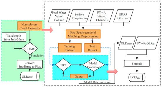
Figure 1.
Flowchart of modeling process and calculation.
3. Results
3.1. Sensitivity Analysis Using SBDART
3.1.1. Total Water Vapor Column
Atmospheric parameters are essential physical quantities that characterize atmospheric conditions. They play a pivotal role in understanding meteorological and climatic phenomena, making weather predictions, and advancing atmospheric science research. The most important atmospheric parameter in the context of longwave radiation is the total water vapor column (TWVC), which refers to the total amount of water vapor in the atmosphere, usually expressed in specific regions or vertical columns. This parameter includes the entire height and all types of water vapor in the atmosphere, including water vapor, liquid water droplets, and ice crystals. The sensitivity of longwave radiation to changes in water vapor levels is crucial for understanding how changes in atmospheric water vapor affect climate change and its feedback mechanisms.
An increase in TWVC enhances the absorption of longwave radiation. Water vapor molecules are particularly effective in absorbing infrared radiation, especially at wavelengths associated with thermal radiation. Figure 2 shows the changes in longwave radiation irradiance (W/m2/μm) corresponding to different TWVC between 0–100 g/cm2 at wavelengths between 3–30 μm, and the values in parentheses in the legend represent the integrated radiation flux values for all bands (equal to ). It can be seen that lower TWVC results in higher values of . The difference in the maximum and minimum radiation values is 82 W/m2 (from a minimum of 160 W/m2 to a maximum of 242 W/m2). The impact of TWVC on is significant and must be included in the input parameters of the algorithm. Higher levels of TWVC also increase the strength of greenhouse effects by capturing more heat in the atmosphere. In contrast, lower water vapor concentrations can lead to the reduced absorption of longwave radiation, allowing more infrared radiation to escape into space, and resulting in enhanced atmospheric radiative cooling. Thus, the impact of water vapor on longwave radiation is a key factor in climate modeling.
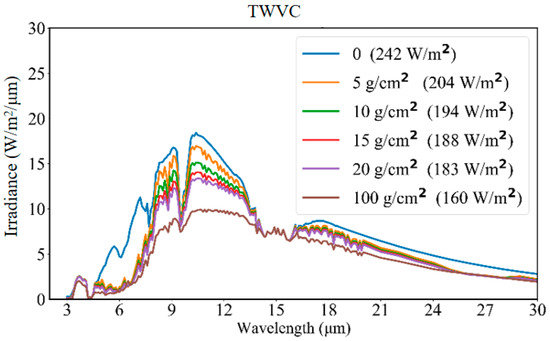
Figure 2.
Longwave radiation irradiance (W/m2/μm) at different atmospheric TWVC (g/cm2) at wavelengths between 3–30 μm. The different colors represent different TWVC, and the values in parentheses in the legend represent the integrated radiation flux values for all bands.
3.1.2. Atmospheric Profiles
In the context of RTMs, the atmospheric profile refers to the variation of several physical atmospheric characteristics with altitude, including temperature, humidity, and pressure. Because these physical atmospheric parameters directly affect the absorption, emission, and scattering of radiation, measuring and analyzing atmospheric profiles can help researchers understand the vertical structure of the atmosphere and reveal differences in meteorological and climatic processes at different altitudes. This information is crucial for simulating and understanding the mechanisms behind radiation transfer processes. Generally, RTMs use built-in atmospheric profile data. Figure 3 presents the impact of different atmospheric profile models on longwave radiation irradiance (W/m2/μm) at wavelengths between 3–30 μm, with each color representing one of six SBDART atmospheric profile models. The figure shows that the tropical model has the highest , followed by the mid-latitude summer, mid-latitude winter, high-latitude summer, high-latitude winter, and the US standard models in descending order. Tropical regions usually have a high incidence of solar radiation, resulting in relatively high surface temperatures; consequently, more longwave radiation is emitted from the surface. In addition, the atmosphere above tropical regions is usually characterized by high water vapor contents and high cloud coverage, which are factors that have a significant impact on .
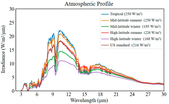
Figure 3.
The impact of six atmospheric profile models included in SBDART on longwave radiation irradiance (W/m2/μm) at wavelengths between 3–30 μm. Each color represents a different atmospheric profile model, and the values in parentheses in the legend represent the integrated radiation flux values for all bands ().
3.1.3. Surface Temperature
Another influential parameter on is surface temperature. Surface temperature has a strong influence on the radiation balance of the Earth’s system. Increases in surface temperature lead to increases in the intensity of surface radiation and, consequently, stronger . Figure 4 presents the variation in longwave radiation irradiance (W/m2/μm) with surface temperature (K) at wavelengths between 3–30 μm. Surface temperatures between 210–330 K were used for this assessment, as this represents the general range of surface temperatures that would be expected on Earth. The figure shows that higher surface temperatures result in greater . The impact of surface temperature on atmospheric longwave radiation is evident and must be included in the input parameters. The changes in surface temperature can also alter the intensity and wavelength of transmitted radiation, which affects the distribution and characteristics of atmospheric longwave radiation.
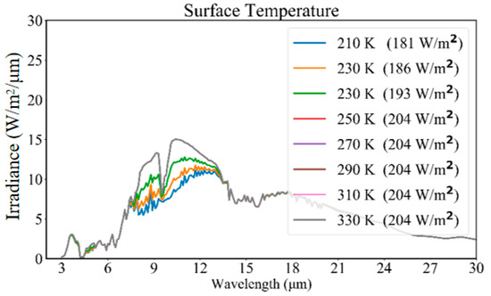
Figure 4.
The variation results of longwave radiation irradiance (W/m2/μm) corresponding to different surface temperatures (K) within the wavelength range of 3 μm–30 μm. The different colors represent different surface temperatures, and the values in parentheses in the legend represent the integrated radiation flux values for all bands ().
3.2. Validation
3.2.1. Quantitative Verification of Results
This study used monthly data from 2018 to quantitatively evaluate the obtained from the AGRI instrument. Figure 5 compares the values obtained from our algorithm with the ERA5 and CERES data recorded in April, August, and December 2018. The results showed that the correlation coefficients of the relationship between the and ERA5 values were 0.92, 0.94, and 0.93 for April, August, and December 2018, respectively. The corresponding MBE and RMSE for each month were 1.87 W/m2 and 5.64 W/m2 in April, 1.43 W/m2 and 4.66 W/m2 in August, 1.46 W/m2 and 4.84 W/m2 in December, respectively. The correlation coefficients of the relationship between the and CERES values were 0.89, 0.91, and 0.90 for April, August, and December 2018, respectively. These results suggest that the values obtained from the AGRI instrument were very close to the values recorded by international mainstream products, and can thus be effectively applied to AGRI data from other international and domestic satellites. In addition, FY-4A has a better spatiotemporal resolution compared to ERA5, allowing for improved capturing of subtle changes. The ERT-based product developed in this study has thus been shown to have high accuracy and has been validated against ERA5 and CERES observations, which indirectly validates the accuracy of any calculated values.
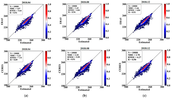
Figure 5.
The values obtained from the algorithm designed in this study and the corresponding ERA5 and CERES data recorded in (a) April, (b) August, and (c) December 2018.
3.2.2. The Spatial Distribution of Results
To validate the detailed spatial distribution of estimates made by the algorithm, the predicted values were compared with different products in smaller localized areas. Figure 6 compares the ERA5, CERES, and the estimated values of in two selected sub-regions. The fact that the low value of OLR in these areas is due to the absorption of longwave radiation from the surface by clouds and the lower temperatures at the cloud top, resulting in lower OLR. Figure 6 shows that the in all three products has relatively similar spatial distributions. It should be noted that the spatial resolution of CERES products is 100 km, making it difficult to distinguish the in these local areas. While the spatial resolution of the ERA5 reanalysis data is better than the CERES products (25-km resolution), its resolution is still relatively coarse. The inversion results obtained by the algorithm developed in this study not only match well with the spatial distribution of the results obtained from CERES but also have a spatial resolution of 4 km, which is significantly better than the ERA5 products. The results of our quantitative evaluation also confirm that the inversion results obtained by our model are closer to the CERES data compared to the ERA5 products and that the accuracy of the product is relatively high. Figure 6 also shows that the resolution of the product obtained by the algorithm is significantly higher than the other two products, just to detect changes in in greater spatial detail. In general, the products from the algorithm developed in this study have a wide coverage, a high spatial resolution, and a 24-h revisit time, providing insights into the study of top-of-atmosphere radiation energy balance.
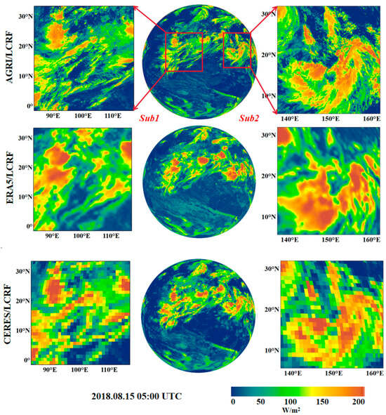
Figure 6.
Analysis of the spatial distribution of instantaneous in two localized sub-regions as described by the algorithm developed in this study, ERA5 reanalysis data, and CERES observations at 05:00 UTC on 15 August 2018.
Long-term trends in radiation levels can be identified by analyzing daily and monthly averages, which can provide researchers with a deeper understanding of the Earth’s energy balance, help monitor climate change processes, and validate meteorological and weather models. Three months’ worth of OLR under all-sky and clear-sky conditions were obtained from the ERA5 and CERES websites and used to calculate the values for these months. Figure 7 shows the spatial distribution of the daily mean values on 1 April, 1 August, and 1 December 2018 as calculated by our algorithm, as well as the values calculated from ERA5 and CERES data during the same period. Once again, the spatial distribution of the values calculated by our algorithm has strong similarities with the results generated by the ERA5 and CERES products. Figure 8 shows the spatial distribution of the monthly average values in April, August, and December 2018 as calculated by our algorithm, ERA5, and CERES data. This figure highlights the stable and reliable results obtained by our model, with values ranging between 0–100 W/m2 over monthly timescales. Figure 8 also shows that clouds have a positive feedback effect on warming, with values ranging from 0–100 W/m2. For example, Australia is located in the southern hemisphere and belongs to a semi-arid and arid climate. Here, the air is relatively dry, and the relatively low water vapor content leads to less cloud formation. Consequently, the Australian region experiences low values across all seasons.
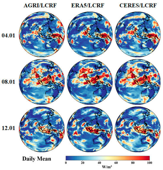
Figure 7.
Spatial distribution of daily mean values obtained from our algorithm compared to the ERA5 and CERES data on 1 April, 1 August, and 1 December 2018.
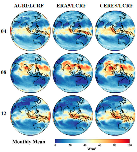
Figure 8.
Spatial distribution of monthly mean values obtained from our algorithm compared to the ERA5 and CERES data on April, August, and December 2018.
3.3. Analysis of Changes
3.3.1. Analysis of Changes Due to Varying Clouds Heights
Clouds at different heights can affect the absorption, reflection, and emission of longwave radiation, and their ability to regulate atmospheric radiation varies greatly; consequently, clouds at different heights have a strong impact on values. A deeper understanding of the changes in caused by different cloud heights will help researchers achieve a greater understanding of the dynamic processes of the climate system, supporting research in meteorology and climate modeling, and helping to address climate change. The cloud top height data employed in this section is derived from the official cloud top height product of the FY-4 satellite. According to the standard of classification of the International Satellite Cloud Climatology Project (ISCCP), clouds are classified into three categories based on their altitude: high, middle, and low clouds. This classification helps in understanding cloud dynamics, energy balance, and their impact on the Earth’s climate. Here are the altitude ranges for each category: High clouds are typically selected above 6500 m and usually found in the middle latitudes. High clouds are composed mainly of ice crystals due to the cold temperatures at these altitudes. Middle clouds generally form between 2000 m and 6500 m. They can be composed of water droplets, ice crystals, or a combination of both, depending on the temperatures present at their altitude. Low clouds are found up to 2000 m above the Earth’s surface. Low clouds are primarily made up of water droplets, although they can also contain ice particles when the temperature is low enough. Figure 9 presents the diurnal variation and frequency distribution of during periods of high-, medium-, and low-height clouds in different months in 2019. High-height clouds are mainly composed of ice crystals with high albedo, while low-height clouds are usually composed of water droplets with relatively low albedo. Therefore, the values are highest during periods of high-cloud conditions, followed by medium- and low-height clouds (Figure 9). This suggests that high-height clouds have the greatest impact on positive radiative forcing. Figure 9 also shows that the range of radiation forcing for clouds of each height is relatively small even over monthly timescales. The second column of Figure 9 shows the frequency distribution of values under different cloud conditions, with the peak density distribution of high-height clouds found at the higher range of values. In contrast, the density distribution curve of the middle-height clouds has a broader peak that falls between the middle range of values, while low clouds have a sharper peak at the lower range of values. These results suggest that high-height clouds exert a greater degree of radiative forcing more frequently, while low-height clouds are more frequently found in the lower forcing range.
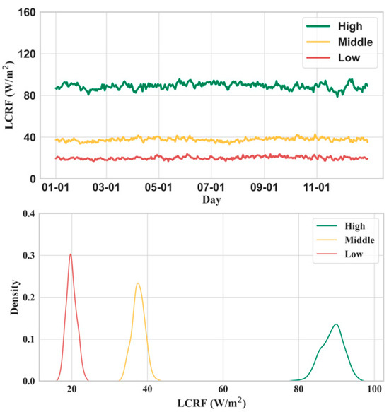
Figure 9.
Diurnal variation of for high-, medium-, and low-height clouds in different months and numerical frequency distribution of at different cloud heights.
3.3.2. Extreme Event Analysis
The high spatiotemporal resolution radiation of the products presents significant advantages for extreme event analysis. These advantages help researchers better understand, monitor, and respond to extreme weather and climate events, which include typhoons, rainstorms, high temperatures, droughts, and floods. These events can significantly change the dynamics and thermodynamic processes of the atmospheric system and have direct and indirect effects on the . For example, rainstorms may lead to a sharp increase in water vapor content in the atmosphere, while also resulting in a wider range of cloud cover. Extreme high-temperature events and extreme low-temperature events can both affect the temperature distribution of the atmosphere, which could potentially lead to increases in surface temperature, changes in the vertical distribution of atmospheric temperature, or the formation of an inversion layer. Due to the close relationship between radiation and temperature, these temperature changes have a direct impact on .
Typhoons are an example of how high spatial resolution radiation data can be helpful for extreme event analysis. Typhoon systems are often accompanied by large-scale cloud clusters and precipitation, which have a strong impact on . In the path of a typhoon, increases in cloud cover lead to a decrease in top-of-atmosphere longwave radiation. Figure 10 shows the distribution of values at different spatial resolutions in typhoon areas at 00:00, 04:00, 08:00, 12:00, 16:00, and 20:00 UTC on 1 October 2018. The figure clearly shows that the changes several times throughout the day due to changes in cloud cover and other atmospheric conditions. The results from this study, as shown in the first panel, have a spatial resolution of 4 km, whereas the corresponding data from CERES, illustrated in the second panel, offer a spatial resolution of only 100 km. When comparing these two sets of images, it becomes evident that the distribution of the typhoon eyes is clearly discernible in the high-resolution images produced by the proposed algorithm. In contrast, such clarity is lacking in the low-resolution images provided by the CERES product.
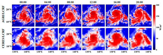
Figure 10.
Comparison of maps generated by the higher-resolution products produced by the proposed algorithm and lower-resolution CERES data in typhoon areas at 00:00, 04:00, 08:00, 12:00, 16:00, and 20:00 UTC on 1 October 2018.
4. Discussion
This paper focuses on assessing , leveraging data from the geostationary FY-4A satellite. A crucial preliminary step involves estimating the OLRclear. The study achieved this by using SBDART, a highly validated and widely used radiative transfer tool, which incorporates DISORT for its multiple scattering radiative transfer calculations. The validity of the methodology is confirmed through comparisons with ERA5 reanalysis data and CERES measurements. The correlation coefficient between the instantaneous values obtained by the proposed algorithm and the corresponding ERA5 product was 0.93 with an RMSE of 5.04 W/m2 and MBE of 1.58 W/m2. In addition, the calculated results were compared to the instantaneous, daily average, and monthly average values obtained from ERA5 and CERES observations. The results show that the product generated from the proposed algorithm had similar spatial distributions to the mainstream products, and had a reasonable degree of agreement with the internationally recognized high-precision CERES radiation results. These results highlight the effectiveness and generalizability of the algorithm to both international and domestic satellites.
The study further presents the diurnal variation and frequency distribution of the during periods of high-, medium-, and low-height clouds in different months in 2019. High-height clouds are mainly composed of ice crystals with high albedo, while low-height clouds are usually composed of water droplets with relatively low albedo. Therefore, the values are highest during periods of high-cloud conditions, followed by medium- and low-height clouds.
The products’ high spatiotemporal resolution radiation offers substantial benefits for analyzing extreme events. These advantages equip researchers with enhanced capabilities to comprehend, monitor, and react to extreme weather and climate phenomena, encompassing typhoons, rainstorms, heatwaves, droughts, and floods. Such events can profoundly alter the dynamics and thermodynamic processes within the atmospheric system, exerting both direct and indirect impacts on the . Typhoons are an example of how high spatial resolution radiation data can be helpful for extreme event analysis. Typhoon systems are often accompanied by large-scale cloud clusters and precipitation, which have a strong impact on . With the results from this study, it becomes evident that the distribution of the typhoon eyes is clearly discernible in the high-resolution images produced by the proposed algorithm. In contrast, such clarity is lacking in the low-resolution images provided by the CERES product.
5. Conclusions
This paper uses the SBDART model to simulate the entire process of how radiation passes through the atmosphere based on the principle of atmospheric radiation transfer. Sensitivity analyses were conducted on important factors such as the surface temperature and total water vapor column, and the quantitative effects of these factors on were calculated. Based on the results of the sensitivity analyses, a highly efficient machine learning method was used to estimate using infrared channels from the AGRI instrument onboard the FY-4A geostationary satellite and was validated against the ERA5 reanalysis data. The FY-4A-based product was intended to provide highly accurate data at higher spatiotemporal resolutions. The correlation coefficient between the instantaneous values obtained by the proposed algorithm and the corresponding ERA5 product was 0.93 with an RMSE of 5.04 W/m2 and MBE of 1.58 W/m2. In addition, the calculated results were compared to the instantaneous, daily average, and monthly average values obtained from ERA5 and CERES observations. The results show that the product generated from the proposed algorithm had similar spatial distributions to the mainstream products, and had a reasonable degree of agreement with the internationally recognized high-precision CERES radiation results. These results highlight the effectiveness and generalizability of the algorithm to both international and domestic satellites.
Author Contributions
Conceptualization, R.X. and J.Z.; methodology, R.X., J.Z., and S.B.; validation, R.X. and L.W.; formal analysis, F.B. and S.B.; resources, R.X. and L.W.; data curation, R.X.; writing—original draft preparation, R.X.; writing—review and editing, R.X. and G.T.; supervision, J.Z. and H.S.; project administration, S.B. and J.Z. All authors have read and agreed to the published version of the manuscript.
Funding
This research was jointly funded by The National Natural Science Foundation of China (Grant 42025504); The Talent Project of Science and Technology in Inner Mongolia under Project no. NJYT24009; and The Startup Fund for Distinguished Scholars under Project no. 2020YJRC052.
Data Availability Statement
The data are available from the authors upon reasonable request as the data need further use.
Acknowledgments
The authors are very grateful to the European Centre for ERA5 (the fifth-generation ECMWF Reanalysis) and CERES SYN data for making the datasets available. The authors also want to thank the National Meteorological Information Center for providing free access to the FY-4A satellite images.
Conflicts of Interest
The authors declare no conflicts of interest.
References
- Shi, G.; Wang, B.; Zhang, H.; Zhao, J.; Tan, S.; Wen, T. The Radiative and Climatic Effects of Atmospheric Aerosols. Chin. J. Atmos. Sci. 2008, 32, 826–840. [Google Scholar] [CrossRef]
- Karpechko, A.Y.; Manzini, E. Stratospheric Influence on Tropospheric Climate Change in the Northern Hemisphere. J. Geophys. Res. 2012, 117, 2011JD017036. [Google Scholar] [CrossRef]
- Hansen, J.; Sato, M.; Kharecha, P.; von Schuckmann, K. Earth’s Energy Imbalance and Implications. Atmos. Chem. Phys. 2011, 11, 13421–13449. [Google Scholar] [CrossRef]
- Intergovernmental Panel On Climate Change Climate Change 2021—The Physical Science Basis: Working Group I Contribution to the Sixth Assessment Report of the Intergovernmental Panel on Climate Change, 1st ed.; Cambridge University Press: Cambridge, UK, 2023; ISBN 978-1-00-915789-6.
- Tang, W.; Qin, J.; Yang, K.; Liu, S.; Lu, N.; Niu, X. Retrieving High-Resolution Surface Solar Radiation with Cloud Parameters Derived by Combining MODIS and MTSAT Data. Atmos. Chem. Phys. 2016, 16, 2543–2557. [Google Scholar] [CrossRef]
- Kato, S.; Rose, F.G.; Rutan, D.A.; Charlock, T.P. Cloud Effects on the Meridional Atmospheric Energy Budget Estimated from Clouds and the Earth’s Radiant Energy System (CERES) Data. J. Clim. 2008, 21, 4223–4241. [Google Scholar] [CrossRef]
- Kandel, R.; Viollier, M. Observation of the Earth’s Radiation Budget from Space. C. R. Geosci. 2010, 342, 286–300. [Google Scholar] [CrossRef]
- Wild, M. The Global Energy Balance as Represented in CMIP6 Climate Models. Clim. Dyn. 2020, 55, 553–577. [Google Scholar] [CrossRef] [PubMed]
- Wild, M.; Folini, D.; Hakuba, M.Z.; Schär, C.; Seneviratne, S.I.; Kato, S.; Rutan, D.; Ammann, C.; Wood, E.F.; König-Langlo, G. The Energy Balance over Land and Oceans: An Assessment Based on Direct Observations and CMIP5 Climate Models. Clim. Dyn. 2015, 44, 3393–3429. [Google Scholar] [CrossRef]
- Johnson, G.C.; Lyman, J.M.; Loeb, N.G. Improving Estimates of Earth’s Energy Imbalance. Nat. Clim. Chang. 2016, 6, 639–640. [Google Scholar] [CrossRef]
- Zhang, X.; Zhao, X.; Li, W.; Liang, S.; Wang, D.; Liu, Q.; Yao, Y.; Jia, K.; He, T.; Jiang, B.; et al. An Operational Approach for Generating the Global Land Surface Downward Shortwave Radiation Product From MODIS Data. IEEE Trans. Geosci. Remote Sens. 2019, 57, 4636–4650. [Google Scholar] [CrossRef]
- Dedieu, G.; Deschamps, P.Y.; Kerr, Y.H. Satellite Estimation of Solar Irradiance at the Surface of the Earth and of Surface Albedo Using a Physical Model Applied to Metcosat Data. J. Appl. Meteorol. Climatol. 1987, 26, 79–87. [Google Scholar] [CrossRef]
- Liang, S.; Wang, D.; He, T.; Yu, Y. Remote Sensing of Earth’s Energy Budget: Synthesis and Review. Int. J. Digit. Earth 2019, 12, 737–780. [Google Scholar] [CrossRef]
- Li, M.; Letu, H.; Peng, Y.; Ishimoto, H.; Lin, Y.; Nakajima, T.Y.; Baran, A.J.; Guo, Z.; Lei, Y.; Shi, J. Investigation of Ice Cloud Modeling Capabilities for the Irregularly Shaped Voronoi Ice Scattering Models in Climate Simulations. Atmos. Chem. Phys. 2022, 22, 4809–4825. [Google Scholar] [CrossRef]
- Wang, D.; Liang, S.; Zhang, Y.; Gao, X.; Brown, M.G.L.; Jia, A. A New Set of MODIS Land Products (MCD18): Downward Shortwave Radiation and Photosynthetically Active Radiation. Remote Sens. 2020, 12, 168. [Google Scholar] [CrossRef]
- Letu, H.; Nakajima, T.Y.; Wang, T.; Shang, H.; Ma, R.; Yang, K.; Baran, A.J.; Riedi, J.; Ishimoto, H.; Yoshida, M.; et al. A New Benchmark for Surface Radiation Products over the East Asia–Pacific Region Retrieved from the Himawari-8/AHI Next-Generation Geostationary Satellite. Bull. Am. Meteorol. Soc. 2022, 103, E873–E888. [Google Scholar] [CrossRef]
- Yu, Y.; Shi, J.; Wang, T.; Letu, H.; Yuan, P.; Zhou, W.; Hu, L. Evaluation of the Himawari-8 Shortwave Downward Radiation (SWDR) Product and Its Comparison With the CERES-SYN, MERRA-2, and ERA-Interim Datasets. IEEE J. Sel. Top. Appl. Earth Obs. Remote Sens. 2019, 12, 519–532. [Google Scholar] [CrossRef]
- Rutan, D.A.; Kato, S.; Doelling, D.R.; Rose, F.G.; Nguyen, L.T.; Caldwell, T.E.; Loeb, N.G. CERES Synoptic Product: Methodology and Validation of Surface Radiant Flux. J. Atmos. Ocean. Technol. 2015, 32, 1121–1143. [Google Scholar] [CrossRef]
- Barkstrom, B.R. The Earth Radiation Budget Experiment (ERBE). Bull. Am. Meteorol. Soc. 1984, 65, 1170–1185. [Google Scholar] [CrossRef]
- Liang, S.; Zheng, T.; Liu, R.; Fang, H.; Tsay, S.-C.; Running, S. Estimation of Incident Photosynthetically Active Radiation from Moderate Resolution Imaging Spectrometer Data. J. Geophys. Res. Atmos. 2006, 111, D15208. [Google Scholar] [CrossRef]
- Doelling, D.R.; Loeb, N.G.; Keyes, D.F.; Nordeen, M.L.; Morstad, D.; Nguyen, C.; Wielicki, B.A.; Young, D.F.; Sun, M. Geostationary Enhanced Temporal Interpolation for CERES Flux Products. J. Atmos. Ocean. Technol. 2013, 30, 1072–1090. [Google Scholar] [CrossRef]
- Lee, H.-T.; Gruber, A.; Ellingson, R.G.; Laszlo, I. Development of the HIRS Outgoing Longwave Radiation Climate Dataset. J. Atmos. Ocean. Technol. 2007, 24, 2029–2047. [Google Scholar] [CrossRef]
- Park, M.-S.; Ho, C.-H.; Cho, H.; Choi, Y.-S. Retrieval of Outgoing Longwave Radiation from COMS Narrowband Infrared Imagery. Adv. Atmos. Sci. 2015, 32, 375–388. [Google Scholar] [CrossRef]
- Govaerts, Y.M.; Arriaga, A.; Schmetz, J. Operational Vicarious Calibration of the MSG/SEVIRI Solar Channels. Adv. Space Res. 2001, 28, 21–30. [Google Scholar] [CrossRef]
- Ma, L.; Liu, Y.; Zhang, X.; Ye, Y.; Yin, G.; Johnson, B.A. Deep Learning in Remote Sensing Applications: A Meta-Analysis and Review. ISPRS J. Photogramm. Remote Sens. 2019, 152, 166–177. [Google Scholar] [CrossRef]
- Hou, N.; Zhang, X.; Zhang, W.; Wei, Y.; Jia, K.; Yao, Y.; Jiang, B.; Cheng, J. Estimation of Surface Downward Shortwave Radiation over China from Himawari-8 AHI Data Based on Random Forest. Remote Sens. 2020, 12, 181. [Google Scholar] [CrossRef]
- Ummenhofer, C.C.; Meehl, G.A. Extreme Weather and Climate Events with Ecological Relevance: A Review. Philos. Trans. R. Soc. B Biol. Sci. 2017, 372, 20160135. [Google Scholar] [CrossRef] [PubMed]
- Ricchiazzi, P.; Yang, S.; Gautier, C.; Sowle, D. SBDART: A Research and Teaching Software Tool for Plane-Parallel Radiative Transfer in the Earth’s Atmosphere. Bull. Am. Meteorol. Soc. 1998, 79, 2101–2114. [Google Scholar] [CrossRef]
- Kim, B.-Y.; Lee, K.-T.; Jee, J.-B.; Zo, I.-S. Retrieval of Outgoing Longwave Radiation at Top-of-Atmosphere Using Himawari-8 AHI Data. Remote Sens. Environ. 2018, 204, 498–508. [Google Scholar] [CrossRef]
- Hersbach, H.; Bell, B.; Berrisford, P.; Hirahara, S.; Horányi, A.; Muñoz-Sabater, J.; Nicolas, J.; Peubey, C.; Radu, R.; Schepers, D.; et al. The ERA5 Global Reanalysis. Q. J. R. Meteorol. Soc. 2020, 146, 1999–2049. [Google Scholar] [CrossRef]
- Gao, J.; Chen, J.; Tian, X. Ensemble-Learning-Based Cloud Phase Classification Method for FengYun-4 Remote Sensing Images. Infrared Technol. 2020, 42, 68–74. [Google Scholar] [CrossRef]
- Smith, G.L.; Priestley, K.J.; Loeb, N.G.; Wielicki, B.A.; Charlock, T.P.; Minnis, P.; Doelling, D.R.; Rutan, D.A. Clouds and Earth Radiant Energy System (CERES), a Review: Past, Present and Future. Adv. Space Res. 2011, 48, 254–263. [Google Scholar] [CrossRef]
- Bao, S.; Letu, H.; Zhao, J.; Shang, H.; Lei, Y.; Duan, A.; Chen, B.; Bao, Y.; He, J.; Wang, T.; et al. Spatiotemporal Distributions of Cloud Parameters and Their Response to Meteorological Factors over the Tibetan Plateau during 2003–2015 Based on MODIS Data. Int. J. Climatol. 2019, 39, 532–543. [Google Scholar] [CrossRef]
- Ri, X.; Husi, L.; Nakajima, T.Y.; Shi, C.; Gegen, T.; Zhao, J.; Zhang, P.; Chen, L.; Shi, J. Cloud, Atmospheric Radiation and Renewal Energy Application (CARE) Cloud Top Property Product from Himawari-8/AHI: Algorithm Development and Preliminary Validation. IEEE Trans. Geosci. Remote Sens. 2021, 60, 4108011. [Google Scholar] [CrossRef]


Disclaimer/Publisher’s Note: The statements, opinions and data contained in all publications are solely those of the individual author(s) and contributor(s) and not of MDPI and/or the editor(s). MDPI and/or the editor(s) disclaim responsibility for any injury to people or property resulting from any ideas, methods, instructions or products referred to in the content. |
© 2024 by the authors. Licensee MDPI, Basel, Switzerland. This article is an open access article distributed under the terms and conditions of the Creative Commons Attribution (CC BY) license (https://creativecommons.org/licenses/by/4.0/).