A Novel Method for Cloud and Cloud Shadow Detection Based on the Maximum and Minimum Values of Sentinel-2 Time Series Images

Abstract

Automatic and accurate detection of clouds and cloud shadows is a critical aspect of optical remote sensing image preprocessing. This paper provides a time series maximum and minimum mask method (TSMM) for cloud and cloud shadow detection. Firstly, the Cloud Score+S2_HARMONIZED (CS+S2) is employed as a preliminary mask for clouds and cloud shadows. Secondly, we calculate the ratio of the maximum and sub-maximum values of the blue band in the time series, as well as the ratio of the minimum and sub-minimum values of the near-infrared band in the time series, to eliminate noise from the time series data. Finally, the maximum value of the clear blue band and the minimum value of the near-infrared band after noise removal are employed for cloud and cloud shadow detection, respectively. A national and a global dataset were used to validate the TSMM, and it was quantitatively compared against five other advanced methods or products. When clouds and cloud shadows are detected simultaneously, in the S2ccs dataset, the overall accuracy (OA) reaches 0.93 and the F1 score reaches 0.85. Compared with the most advanced CS+S2, there are increases of 3% and 9%, respectively. In the CloudSEN12 dataset, compared with CS+S2, the producer’s accuracy (PA) and F1 score show increases of 10% and 4%, respectively. Additionally, when applied to Landsat-8 images, TSMM outperforms Fmask, demonstrating its strong generalization capability.

1. Introduction

The loss of information due to clouds and cloud shadows is a widespread issue, significantly impacting various subsequent research applications such as land cover and change detection, atmospheric variable estimation, and ocean parameter inversion [1,2,3,4,5,6]. As a result, the detection of clouds and cloud shadows has become the primary challenge for many passive remote sensing satellite image production applications [7,8,9,10]. The international satellite cloud climatology project estimates that the global average annual cloud cover is as high as 66%. For continuous observation of massive data from satellites such as Landsat and Sentinel-2 series satellites, archived images often contain numerous clouds and cloud shadows. Detecting thick clouds or deep shadows is relatively straightforward due to their high or low reflectivity in the visible light band [7]. However, detecting thin clouds or shallow shadows poses significant challenges, as their signals closely resemble those of ground objects and are difficult to distinguish [11,12,13]. While manual drawing of clouds and cloud shadows yields high accuracy, it is also extremely time consuming. With Landsat alone capturing over 1 million photos per month, manual annotation becomes impractical, especially within the context of “Earth Big Data” [14,15].

In recent years, numerous methods for cloud and cloud shadow detection have been proposed. Many classical methods have been applied to satellites such as MODIS, Landsat, and Sentinel-2, yielding various cloud and cloud shadow products [16]. Cloud and cloud shadow detection methods can be categorized into three groups based on the number of images utilized: single-temporal, temporal, and learning models [17]. Single-temporal methods typically establish thresholds based on the physical characteristics of clouds. For instance, the MODIS cloud mask [18] utilizes multiple cloud detections to assess the likelihood of clear skies, employing a series of thresholds to conduct various spectral tests on pixels, resulting in multiple pixel classifications. The United States Geological Survey (USGS) has employed the automatic cloud coverage assessment ACCA [19] and the mask function Fmask [20,21,22] as the cloud and cloud shadow detection methods for Landsat. ACCA estimates the cloud coverage percentage in each Landsat image by utilizing multiple spectral filters, with particular emphasis on the thermal infrared band. On the other hand, Fmask integrates various bands, including cirrus bands, digital elevation model (DEM), global water mask, snow detection, etc. Fmask demonstrates accurate cloud and cloud shadow detection capabilities across various complex scenes in Landsat and Sentinel-2 imagery. The cloud displacement index CDI further supplements the cloud detection theory [21]. In addition to considering spectral characteristics, CDI also incorporates Sentinel-2’s systematic observation structure to accurately distinguish bright objects from clouds based on band parallax. The successful application of CDI in cloud detection in large urban areas is integrated into the Fmask and Force frameworks. Sen2Cor [23] was developed by the European Space Agency (ESA) for atmospheric correction of the Sentinel-2 satellite. The resulting scene classification map (SCL), with identifiers such as cloud, cloud shadow, cirrus, and snow probability, can also be used for cloud and cloud shadow detection.

The multi-temporal method incorporates the characteristics of the time dimension, assuming that the ground objects generally change slowly over seasons or periods [24]. Cloud and cloud shadow recognition is achieved by detecting changes in the time series of images [25]. Compared with the single-phase method, the time series method benefits from time information and further enhances the capability of cloud and cloud shadow detection [20]. Multi-temporal cloud detection (MTCD) [10] combines adjacent temporal pixels to capture the sharp increase in reflectivity of the blue band for cloud detection. This method yields good results for thick clouds and demonstrates a certain level of effectiveness for detecting thin clouds. The multi-temporal mask, Tmask [20], extends the principles of Fmask by incorporating a green band, near-infrared band, and short-wave infrared band. The sine–cosine time series model of each pixel is constructed using iterative weighted least squares, significantly enhancing the detection capability for cloud shadows of thin clouds. Lin [25] proposed a multi-temporal cloud detection method based on invariant pixels. The invariant pixels are extracted using weighted principal component analysis. Luis Gómez-Chova [26] proposed a linear and nonlinear least squares regression method to minimize both prediction and estimation errors. This method is implemented in GEE and is suitable for a global scale.

With the development of computer performance and theory, machine learning (ML) and deep learning (DL) have become increasingly prominent. S2cloudless is a ML method for automatic cloud detection in single-temporal Sentinel-2 images, based on a gradient enhancement algorithm. Through semantic segmentation using a convolutional neural network, the probability of cloud coverage is assigned to each pixel by combining their spectral features [9]. InterSSIM is a multi-temporal version of S2cloudless, which considers both the temporal and spatial context and selects the most important features using LightGBM. Chai [27] proposed a single-phase deep learning method for cloud and cloud shadow detection based on deep convolutional neural networks (CNNs). This method treats cloud and cloud shadow detection as a semantic segmentation problem. The multi-level spatial and spectral features of the successively convolutional and deconvolutional images are utilized to achieve detailed segmentation, with each pixel classified as cloud, thin cloud, cloud shadow, or clear. Using a Generative Adversarial Network (GAN) for image restoration is a common task in computer vision [28]. Its generator (G) and discriminator (D) are trained to be consistent with each other and have been successfully applied to cloud detection [29]. Meng [30] combined GAN with an attention mechanism to fully capture the characteristics of clouds. In view of the complex cloud distribution, Wu [13] proposed an extensible boundary network to fuse multi-scale cloud masks, and the differential cloud masks were obtained by the differential boundary network. Cloud Score+ (CS+) [31] is a quality evaluation processor developed using a weakly supervised joint spatio-temporal context video deep learning method with approximately 2.2 million training images. Temporal images of the same location are utilized as video training to generate a clear reference image for image quality assessment. CS+ has been implemented in Sentinel-2 to generate cloud products CS+S2, enabling effective detection of both clouds and cloud shadows by adjusting the quality parameters.

Most existing cloud and cloud shadow detection methods suffer from incomplete detection of thick-cloud-depth shadows and missed detection of thin clouds and shallow shadows [22,32]. The current research predominantly focus on cloud detection, with limited attention given to specific cloud shadow detection methods [6] due to the inherent difficulty of detecting cloud shadows. In general, single-temporal-based methods rely solely on spectral features and do not consider spatial features such as texture [33]. Thresholds are set based on human experience, making it difficult to handle complex surface and cloud types [34]. The method based on the time series model considers the temporal dimension, resulting in significant improvement compared to the single-phase method. However, it may mistakenly identify rapidly changing ground objects as clouds or cloud shadows. While the learning-based method has achieved high detection accuracy, raining the model requires a large amount of high-quality sample data [35]. Balancing the convergence between training data and sample data necessitates computing resources with high memory [36]. Furthermore, developing a common paradigm or model to address diverse clouds poses a challenge. Generalizing the model to various sensors and research domains is also a significant challenge.

In this paper, the TSMM for cloud and cloud shadow detection, considering temporal characteristics, is proposed. This method utilizes the blue band and near-infrared band to estimate the temporal features and incorporates the spatial convolution operation to fully leverage the complementary advantages of temporal, spatial, and spectral information. This approach further enhances the accuracy of cloud and cloud shadow detection. Experiments have shown that this method is not only applicable for cloud and cloud shadow detection in Sentinel-2 imagery across various underlying surface scenes, but also for detecting clouds and cloud shadows in remote sensing images captured by other sensors. It can generate more accurate and comprehensive cloud and cloud shadow products for more passive sensors.

2. Data

2.1. Sentinel-2 MSI

The Sentinel-2 Multi-Spectral Instrument (Sentinel-2 MSI) comprises Sentinel-2A and Sentinel-2B. The two satellites are in a 180° phase difference, with a revisit period of 5 days, even up to 2–3 days [37,38]. The Sentinel-2 user product level is divided into Level-1B, Level-1C, and Level-2A. The Level-1B product represents the radiance at the top of the atmosphere after radiometric correction in sensor geometry, primarily intended for expert users. The Level-1C product represents the top-of-atmosphere reflectance after radiometric correction and spatial registration in cartographic geometry. The Level-2A product is the surface reflectance after atmospheric correction based on the Level-1C product [39]. Since December 2018, ESA has employed Sen2Cor for systematic atmospheric correction on Sentinel-2 images worldwide to generate Level-2A products [40]. Level-2A contains 21 bands, an increase of 8 product bands compared to Level-1C [23]. Among them, AOT, WVP, and SCL are generated based on Sen2Cor. SCL contains 11 scene classification maps, where SCL = 3, 7, 8, 9 are the identifiers of cloud shadow, low-probability cloud, medium-probability cloud, and high-probability cloud, respectively. In this paper, Sentinel-2 Level-2A images are selected for the experimental data.

CS+S2 is selected for the auxiliary data in this paper. CS+S2 is a mask product (resolution 10 m) for assisting Sentinel-2 Level-1C cloud and cloud shadow detection. It provides two products, cs and cs_cdf. The cs band is an atmospheric similarity score with clear pixels and is more sensitive to haze and cloud edges. The possible cs value of the cs_cdf band cumulative distribution function is not sensitive to small changes in spectral values or terrain shadows. We selected the cs_cdf band for the experiment, with a recommended quality parameter of 0.65 [31].

2.2. S2ccs Dataset

S2ccs is a self-made dataset of cloud and cloud shadow imagery encompassing seven Chinese research areas (Figure 1).

Table 1. The study area included in the S2ccs dataset and the proportion of cloud and cloud shadows.

Code	Study Area	Center Coordinates	Timing Image Date (2022)	Label Date and Proportion of Cloud and Cloud Shadow (2022)	Main Type
A	Changchun	(125.39, 44.34)	23 April–3 June 12 May–22 June	05.13 (15%) 06.02 (26%)	Farmland
B	Dunhuang	(99.64, 40.17)	27 February–7 April 13 June–23 July	03.17 (8%) 07.03 (30%)	Gobi beach
C	Chengdu	(104.17, 30.81)	9 April–19 May 5 July–25 July	04.29 (85%) 07.25 (15%)	Buildings
D	Wuhan	(114.25, 30.59)	2 April–12 May 11 July–21 August	04.22 (26%) 07.31 (32%)	Buildings
E	Ningbo	(21.23, 30.37)	9 July–19 August 31 August–10 October	07.29 (42%) 09.20 (39%)	Wetlands
F	Hangzhou	(119.11, 29.58)	4 March–14 April 15 August–25 September	03.24 (3%) 09.05 (88%)	Water and vegetation
G	Hong Kong	(114.24, 22.25)	4 January–14 February 22 February–2 April	01.24 (38%) 03.12 (43%)	Vegetation and ocean

shows the case of the S2ccs dataset, providing additional examples of rare multi-temporal cloud and cloud shadow datasets in the field. Clouds include thick clouds and thin clouds, and cloud shadows include deep shadows and light shadows. The land cover types include vegetation, water, city, farmland, wetland, and gobi beach. The temporal resolution of each region is approximately 2–3 days, and the image set is uniformly cropped to around 557 × 558 pixels. Two scenes were selected from each study area, for a total of 14 scenes. The proportion of clouds and cloud shadows in these scenes ranged from 3% to 88%. After expert visual interpretation, the author manually assigned labels of 1 (clear), 2 (cloud shadow), and 3 (cloud), respectively, to create one of the verification datasets used in this paper.

2.3. CloudSEN12 Dataset

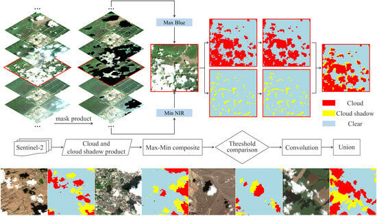
CloudSEN12is a large global dataset (about 1 TB) for cloud semantic understanding, consisting of 49,400 image blocks [41]. These image patches are evenly distributed over all continents except Antarctica. Covering 509 × 509 pixels, each scene was shot from 2018 to 2020. It contains 1C- and 2A-level data from Sentinel-2. Each region of interest has five image blocks on different dates. The cloud and cloud shadow contents correspond to no clouds (0%), almost clear (0–25%), low clouds (25–45%), medium clouds (45–65%), and cloudy (>65%). CloudSEN12 contains 10,000 high-quality label images with label types of 0 (clear), 1 (thick cloud), 2 (thin cloud), and 3 (cloud shadow). In this paper, 1000 scenes are randomly selected as the second verification dataset. Figure 2 shows images of representative features in seven regions.

3. Method

TSMM first masks the sequence images based on CS+S2. Then, TSMM composites the maximum value of the blue band and the minimum value of the near-infrared band in the time series. We remove the time series noise by counting the proportion of the maximum and sub-maximum values of the blue band in the time series and the proportion of the minimum and sub-minimum values of the near-infrared band in the time series. Finally, the clear blue band and the near-infrared band after noise removal are used to detect clouds and cloud shadows, respectively. The misclassified pixel of the detection results is optimized through convolution operations, and we further extract the complete clouds and cloud shadows. In the mask process, the cloud mask is given the highest priority, followed by the cloud shadow mask, with the lowest priority. The specific technical flowchart is depicted in Figure 3.

3.1. Preprocessing

First, we prepare the Sentinel-2 Level-2A image $I^t\left(\mathrm{m}\times \mathrm{n}\right)$ detected at time t. The length of each time series before and after $I^t$ is $T$ days ($5\le T\le 60$, recommended $T=20$), and they are compiled into a time series image dataset $D$. $D$ contains a total of d images. We use the CS+S2 cs_cdf band as the mask to obtain the initial cloud and cloud shadow mask file $M_0$ for each phase. Using Formula (1), we apply $M_0$ to the time series image $D$ to obtain the preliminary mask time series image $D_{pre}$:

$$D_{pre}^t=D^t\times M_0^t,t=\mathrm{1,2},\dots ,t,\dots ,d-1,d.$$

(1)

where $D_{pre}^t$ represents the image at time t of $D_{pre}$, $D^t$ represents the image at time t of D, and $M_0^t$ represents the image at time t of $M_0$.

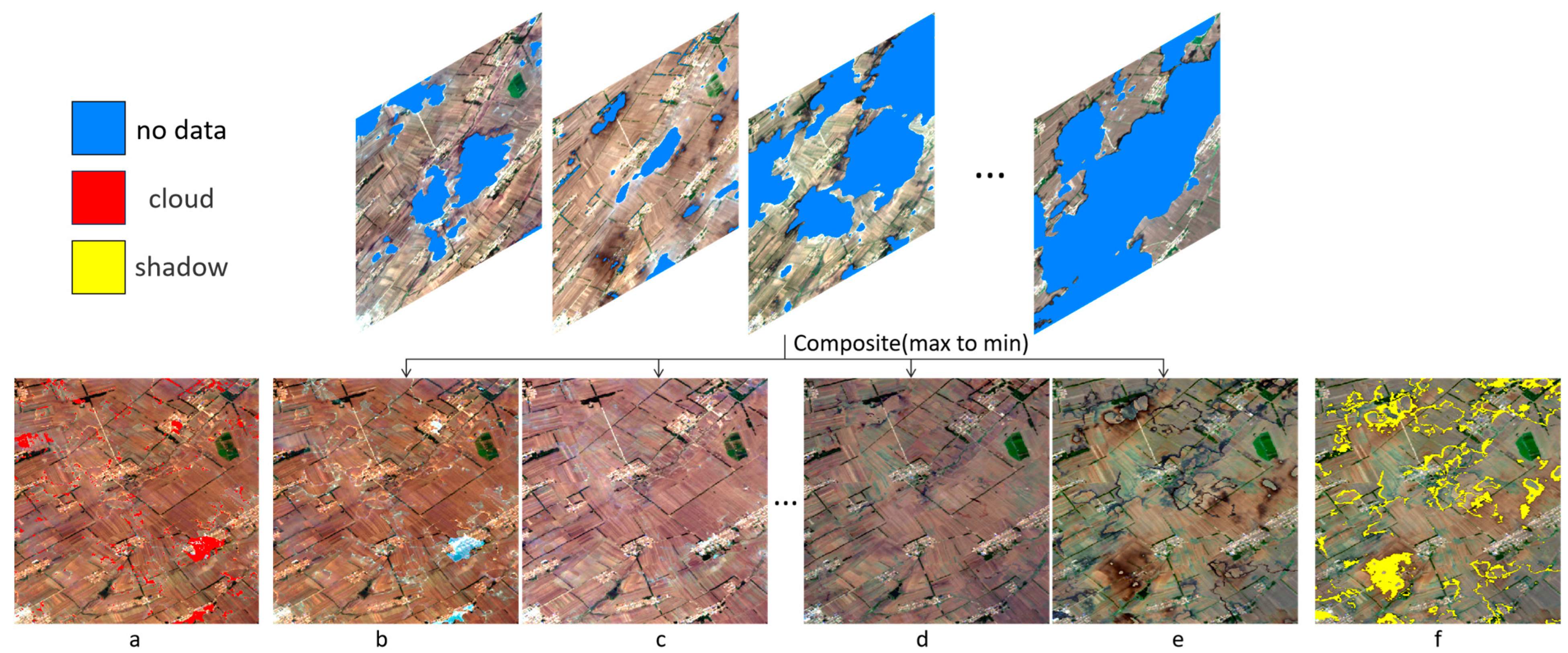
3.2. Maximum and Minimum Value Composite

Considering that clouds are most sensitive in the blue band and cloud shadows are most sensitive in the near-infrared band, we chose the blue band for cloud detection [10] and the near-infrared band for cloud shadow detection [7]. We composited the sorted sequence images of the blue band and the near-infrared band to select the maximum and sub-maximum values of the blue band, as well as the minimum and sub-minimum values of the near-infrared band.

To ensure the maximum removal of clouds and cloud shadows in the composite image, we conducted noise removal. The purpose of the maximum and minimum value composite was to identify the extreme value range of each pixel in the time series, with values exceeding this range considered as the cloud or cloud shadow pixels. However, due to the imperfections of cloud and cloud shadow products, a significant amount of cloud noise may still have been present in the maximum composite image (Figure 4a,b). But the sub-maximum composite image was almost clear (Figure 4c). In this paper, we compare the ratio between the maximum and sub-maximum composite image of the blue band pixel by pixel. If the ratio exceeds the specified multiple ratio $\sigma$(recommended $\sigma =1.2$), the maximum value is likely to be a cloud pixel.

Similarly, the existing cloud shadow detection methods cannot completely detect cloud shadows; the shallow cloud shadow boundary is especially difficult to determine. It is rare for the same cloud shadow to appear in the same location at different times. The minimum composite image usually contains cloud shadow noise (Figure 4e,f), and the sub-minimum composite image is almost clear (Figure 4d). This paper compares the ratio between the sub-minimum and the minimum composite image in the near-infrared band. If the ratio is greater than $\sigma$(recommended $\sigma =1.2$), the minimum value is likely to be a cloud shadow pixel. After comparison, we replace the maximum value identified as the cloud pixel with the sub-maximum value, and replace the minimum value identified as the cloud shadow pixel with the sub-minimum value. The maximum (including sub-maximum) and minimum (including sub-minimum) composite images can better represent the extreme value of each pixel in the time series. Therefore, we define the processed images as the maximum image $A_{Blue\_max}$ in the blue band and the minimum image $A_{NIR\_min}$ in the near-infrared band.

3.3. Cloud and Cloud Shadow Extraction

To detect the cloud and cloud shadow of $I^t$, we compare the blue band $I_{Blue}^t$ and the near-infrared band $I_{NIR}^t$ to $A_{Blue\_max}$ and $A_{NIR\_min}$ of $I^t$, respectively. Through the discrimination of Formulas (2) and (3), we obtain the cloud mask $M_{cloud}^t$ and cloud shadow mask $M_{shadow}^t$ of $I^t$:

$$M_{cloud}^t\left(i,j\right)=\left\{\begin{array}{c}1,I_{Blue}^t\left(i,j\right)>A_{Blue\_max}\left(i,j\right),\\ 0,I_{Blue}^t\left(i,j\right)\le A_{Blue\_max}\left(i,j\right),\end{array}\right. i=\mathrm{0,1},\dots ,m;j=\mathrm{0,1},\dots ,n.$$

(2)

$$M_{shadow}^t\left(i,j\right)=\left\{\begin{array}{c}1,I_{NIR}^t\left(i,j\right)<A_{NIR\_min}\left(i,j\right),\\ 0,I_{NIR}^t\left(i,j\right){\ge A}_{NIR\_min}\left(i,j\right),\end{array}\right. i=\mathrm{0,1},\dots ,m;j=\mathrm{0,1},\dots ,n.$$

(3)

where $M_{cloud}^t\left(i,j\right)$ represents the cloud file, $M_{shadow}^t\left(i,j\right)$ represents the cloud shadow file, $I_{Blue}^t\left(i,j\right)$ represents the pixel value of row $i$ and column $j$ of the blue band of the image, $I_{NIR}^t\left(i,j\right)$ represents the pixel value of row $i$ and column $j$ of the near-infrared band of the image, 1 represents cloud or cloud shadow pixels, and 0 represents clear pixels.

Although the above steps accurately identify the cloud and cloud shadow pixels and their boundaries, the results may exhibit misclassified pixels. The main reason is that some clear, bright pixels are identified as cloud pixels, while some clear, dark pixels are identified as cloud shadow pixels. For example, during periods of high temperature and cloudy weather, the reflectivity of certain ground objects may exceed the maximum value due to prolonged irradiation. Similarly, in the aftermath of rain, the water content of some ground objects increases, leading to lower reflectivity than the minimum value. Considering the spatial characteristics, areas surrounding a cloud pixel center are more likely to be cloud pixels, while areas surrounding a clear pixel center are more likely to be clear pixels. To remove the misclassified pixels, this paper introduces the convolution kernel $K$ to convolution the cloud mask and cloud shadow mask, respectively. Through the discrimination of Formulas (4) and (5), we calculate the mean value of the center pixel neighborhood. When the mean value is greater than or equal to $\mu$ (recommended $\mu =0.3$), the center pixel is cloud or cloud shadow, and the discriminant value is 1. Otherwise, it is a clear pixel, and the discriminant value is 0. The convolution cloud mask $M_{cloud\_conv}^t$ and the convolution cloud shadow mask $M_{shadow\_conv}^t$ are obtained as follows:

$$M_{cloud\_conv}^t\left(i,j\right)=\left\{\begin{array}{c}1,{mean(M}_{cloud}^t\ast K)\left(i,j\right)\ge \mu ,\\ 0,{mean(M}_{cloud}^t\ast K)\left(i,j\right)<\mu ,\end{array}\right.i=\mathrm{0,1},\dots ,m;j=\mathrm{0,1},\dots ,n.$$

(4)

$$M_{shadow\_conv}^t\left(i,j\right)=\left\{\begin{array}{c}1,{mean(M}_{shadow}^t\ast K)\left(i,j\right)\ge \mu ,\\ 0,{mean(M}_{shadow}^t\ast K)\left(i,j\right)<\mu ,\end{array}\right.i=\mathrm{0,1},\dots ,m;j=\mathrm{0,1},\dots ,n.$$

(5)

4. Experiment

4.1. Sensitivity Experiments

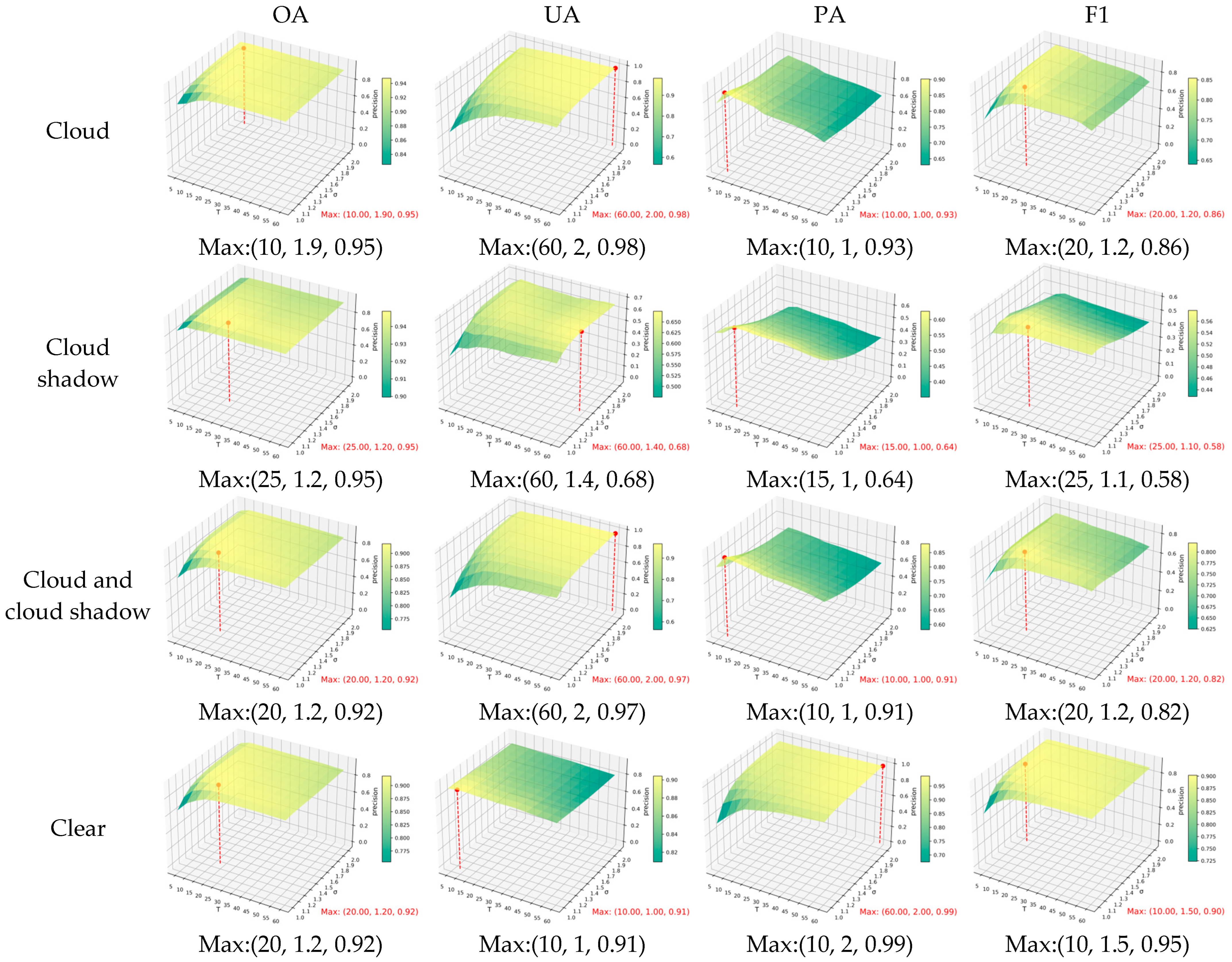
4.1.1. Time Series Length and Max–Min Magnification

The number of time series images varies according to their time series characteristics, and the ratio of maximum to minimum values within sequences of different lengths also exhibits varying characteristics. An appropriate time series length means reasonable temporal variation characteristics. To achieve optimal temporal characteristics, TSMM proposes the time series length of T days and the maximum magnification σ as the first set of parameters. As shown in Figure 5, the X axis represents $T$, the Y axis represents $\sigma$, and the Z axis represents the accuracy index. The three parameters form a combination of ($T$, $\sigma$, accuracy index). The time series length range of $T$ is 5~60, and the interval is 5. The value range of $\sigma$ is 1~2, and the interval is 0.1. The trend of accuracy evaluation of cloud detection is almost identical to that of cloud and cloud shadow detection, as the proportion of cloud is greater than that of cloud shadow. From OA and F1, we observe that when $T$ ranges from 5 to 20, the accuracy of TSMM shows rapid improvement. In the range of 20 to 30, TSMM performs well. However, when $T$ exceeds 30, the accuracy of TSMM decreases slowly. When $\sigma$ increases from 1 to 1.2, the accuracy of TSMM increases rapidly. In the range of 1.2 to 1.4, the accuracy of TSMM remains stable. However, when $\sigma$ > 1.4, the accuracy of TSMM decreases slowly. The optimal cloud and cloud shadow F1 with $T$= 20 and $\sigma$= 1.2 are selected as the recommended parameters.

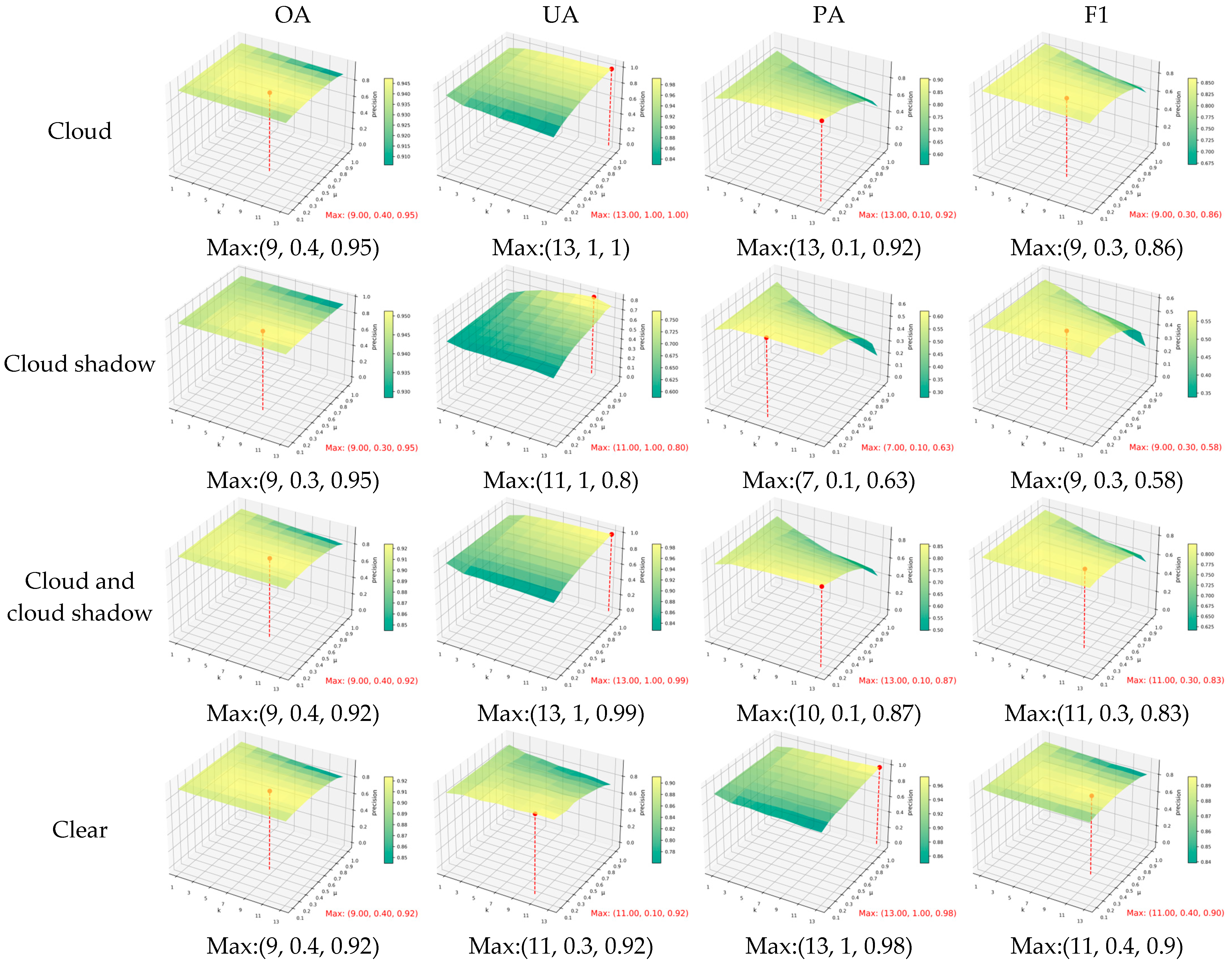
4.1.2. Convolution Kernel Size and Neighborhood Mean

To reduce misclassified pixels, TSMM introduces a convolution kernel to calculate the neighborhood mean of the mask. We take the convolution kernel size $k$ and the average threshold $\mu$ as the second set of parameters. As shown in Figure 6 the X-axis represents $k$, the Y-axis represents $\mu$, and the Z-axis represents the accuracy index. The three parameters form a combination of ($k$, $\mu$, accuracy index). The value range of $k$ is from 1 to 13, with an interval of 2. The value range of $\mu$ is from 0.1 to 1, with an interval of 0.1. When $k$ ranges from 1 to 3, only a small amount of spatial information is utilized, resulting in a low accuracy of TSMM. However, when $k$ ranges from 5 to 13, its computational field of view gradually increases, leading to a stable and excellent performance of TSMM. When $\mu$ ranges from 0.1 to 0.4, the spatial information is fully utilized, allowing TSMM to achieve stable, high-precision performance. However, when $\mu$ is greater than 0.4, the accuracy of TSMM gradually decreases. The optimal cloud and cloud shadow F1 with $k$= 11 and $\mu$= 0.3 are selected as the recommended parameters.

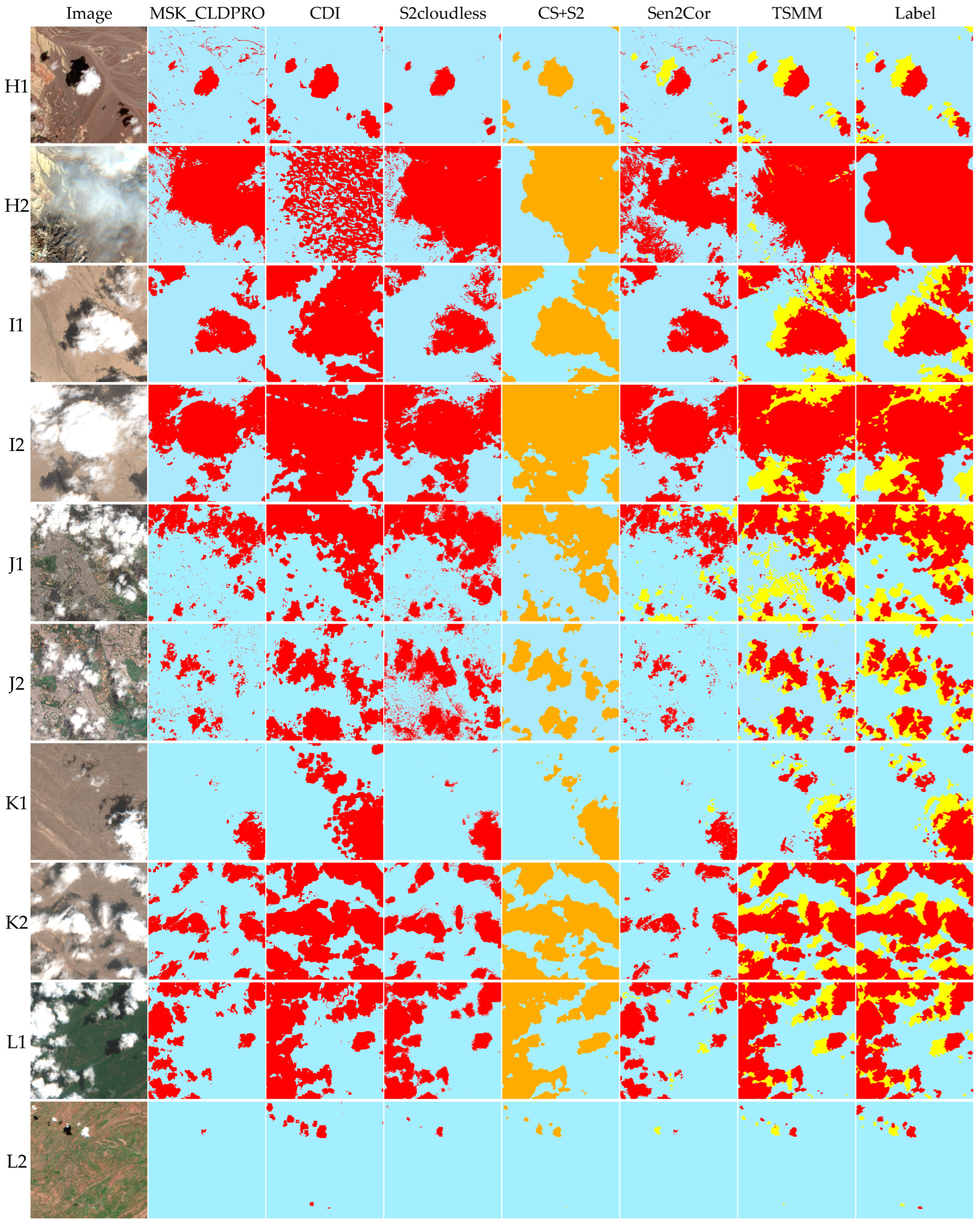
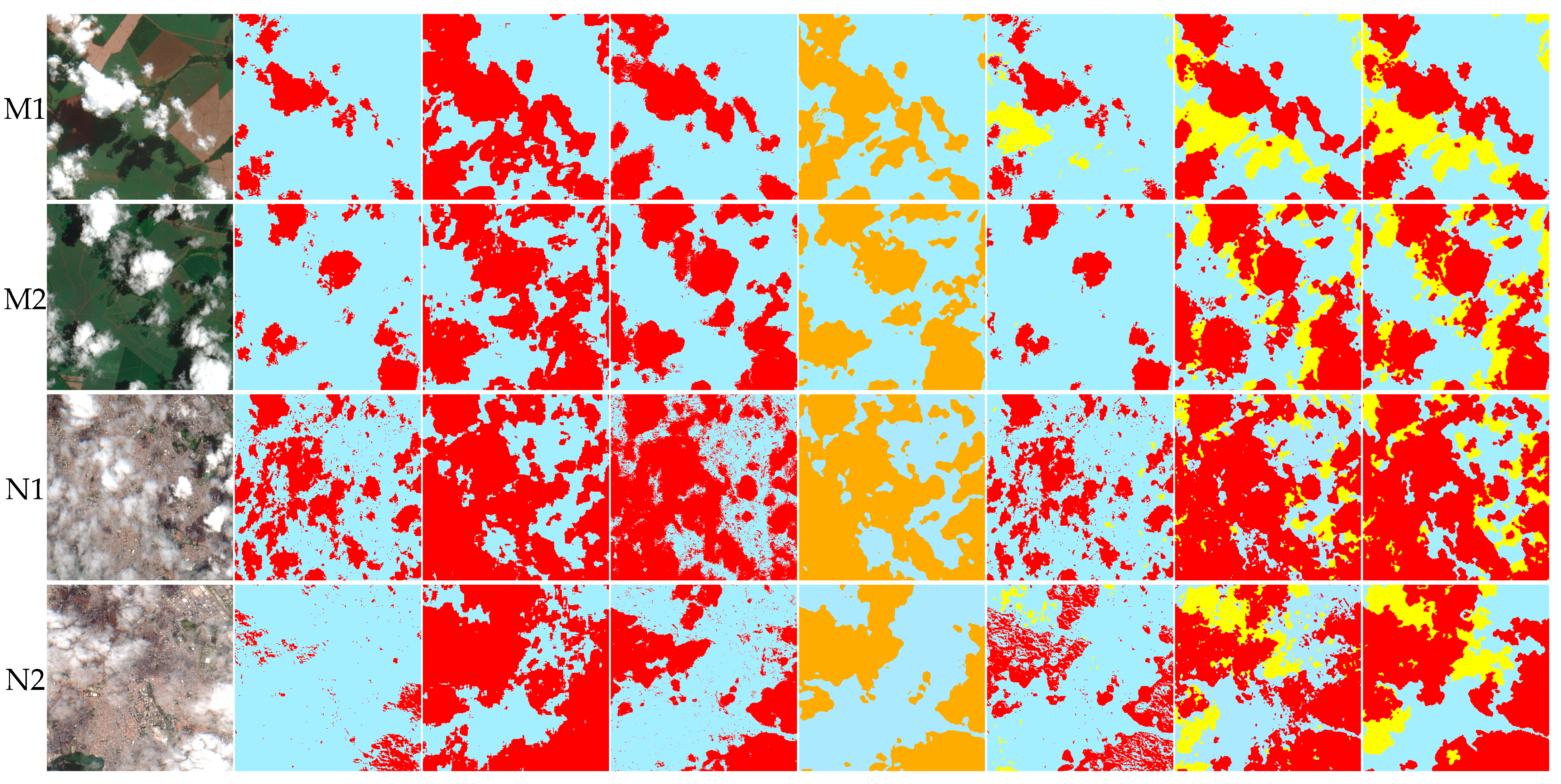
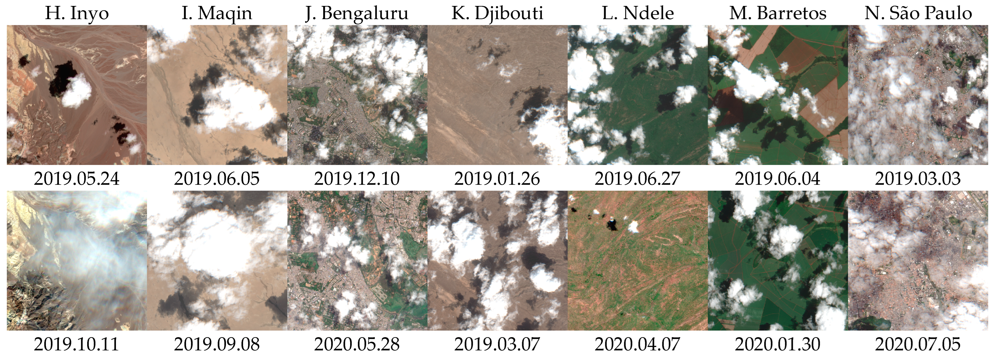
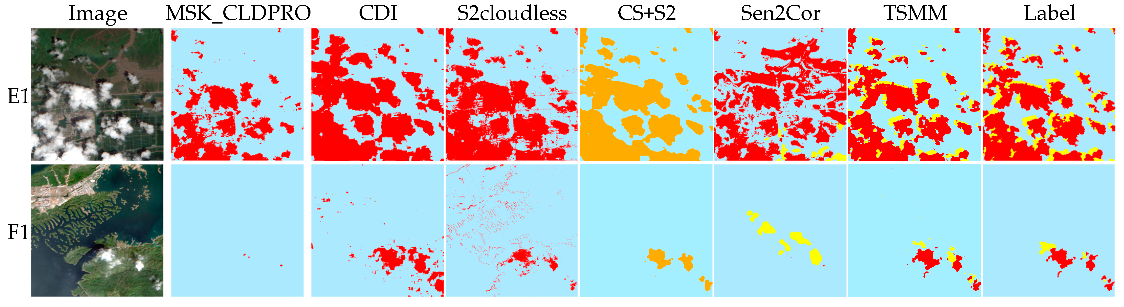
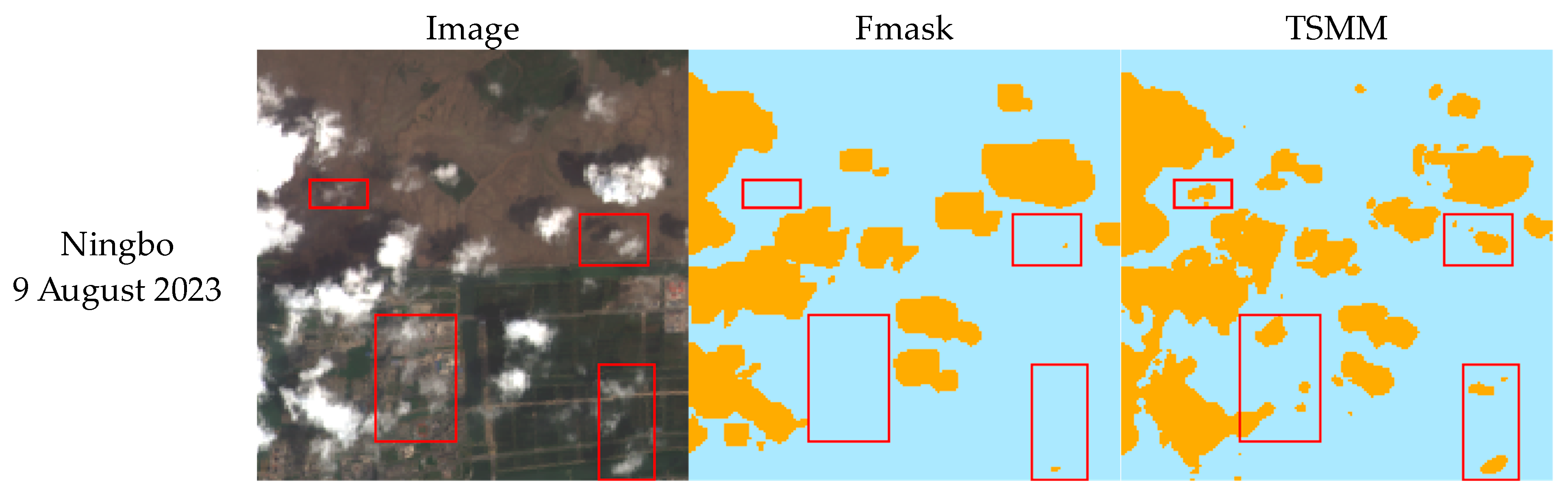
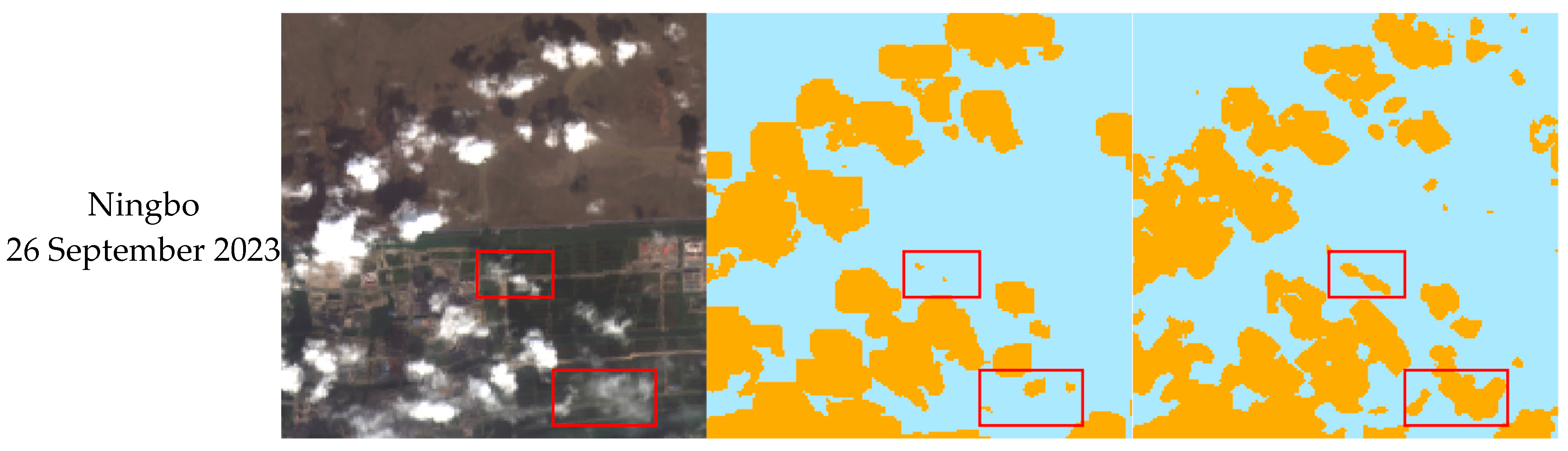
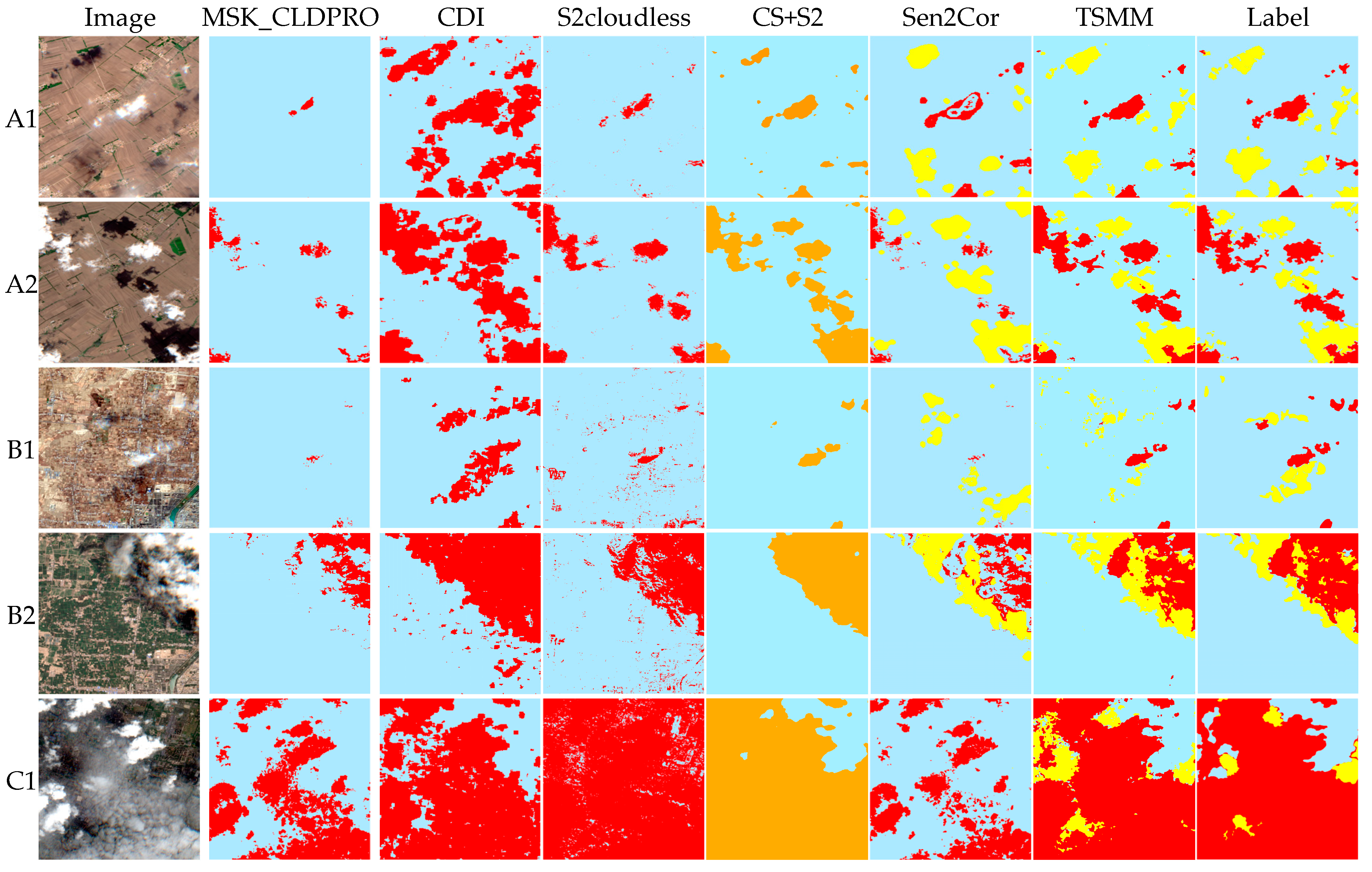
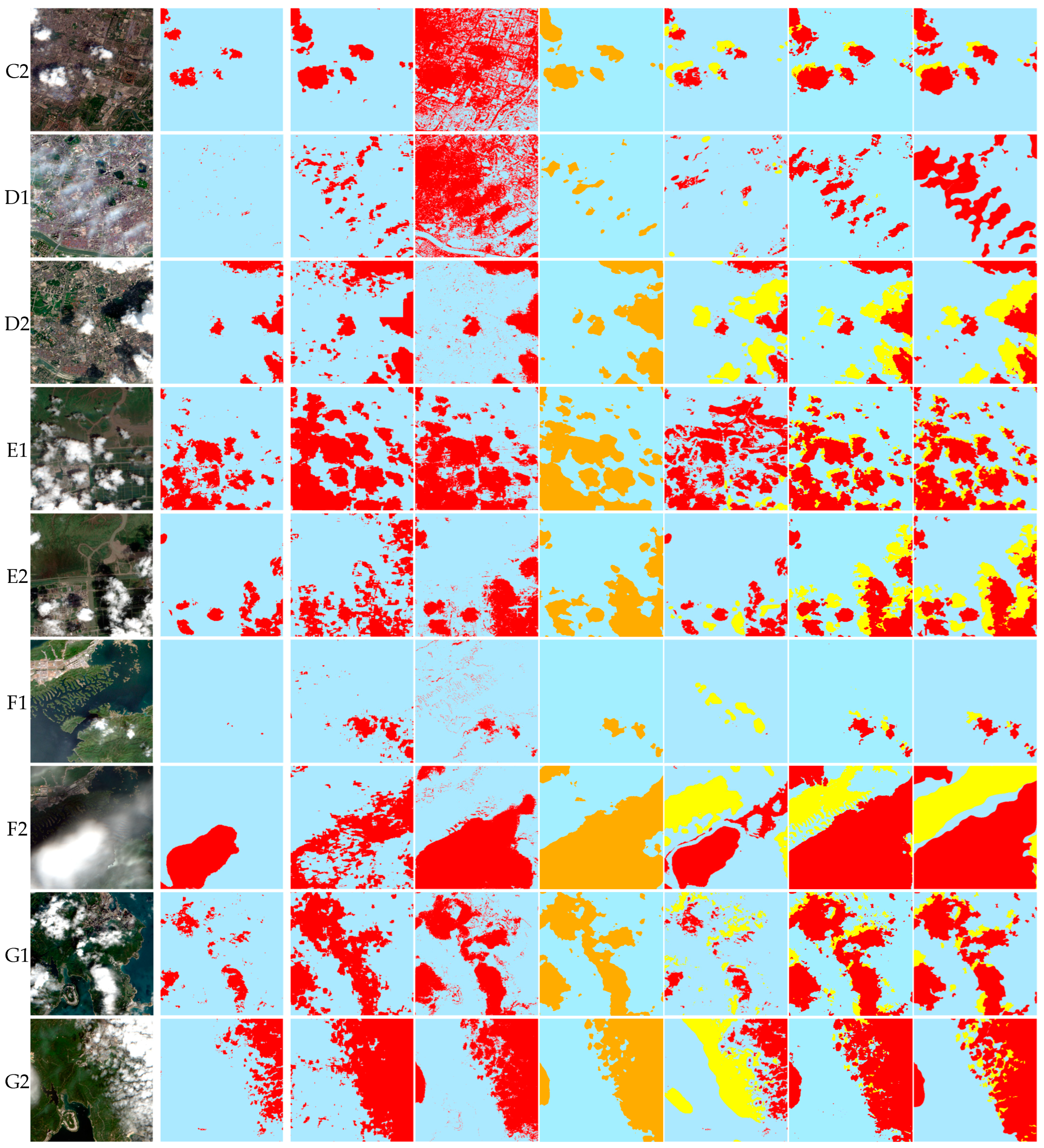
4.2. Qualitative Assessment

To better verify the effectiveness and advancement of the proposed method, we selected TSMM to compare with five other advanced methods or products.

MSK_CLDPRO is the official global cloud product band of Sentinel-2A with a resolution of 20 m. CDI is an excellent detection algorithm integrated in the Fmask and Force framework, and CDI is its cloud product. S2cloudless is an excellent machine learning algorithm, and the probability band is its cloud product. CS+ is one of the most advanced algorithms for Sentinel-2A, and CS+S2 is its cloud and cloud shadow product. Sen2cor is the official quality processor, and SCL is its product. It is divided into high-probability clouds (SCL = 9), medium-probability clouds (SCL = 8), low-probability clouds (SCL = 7) and cloud shadows (SCL = 3). Note that only Sen2cor and TSMM provide separate cloud and cloud shadow detection; CS+ detects cloud and cloud shadow together, and other methods only provide cloud detection. In the S2ccs dataset, the manual labels are 1 (clear), 2 (cloud shadow), and 3 (cloud). Labels are used as the basis for the classification of truth values and accuracy evaluation.

Figure 7 shows the results of the S2ccs dataset, while Figure 8 shows the results of seven representative regions from the CloudSEN12 dataset. MSK_CLDPRO has more missed detections, as it focuses on detecting thick clouds and tends to ignore thin clouds. CDI has more false detection, as it detects the cloud and expands outward. It often misidentifies cloud shadows as clouds, and is not effective in detecting thin clouds. When appropriate cloud probability parameters are selected, S2cloudless demonstrates powerful cloud detection ability. However, this method often misidentifies a large number of highlighted scenes as clouds, resulting in significant noise. CS+ demonstrates powerful performance, with the results closely matching the labels. However, CS+ lacks the ability to distinguish between clouds and cloud shadows separately, resulting in missed detections of some thin clouds and shallow shadows. Although Sen2cor provides separate cloud and cloud shadow detection, both are mediocre, and Sen2cor often misses thin clouds and cloud shadows.

In the S2ccs dataset (Figure 7, specifically shown in Appendix A, Figure A1), TSMM performs very stably in complex scenarios. For example, when there are thin clouds over the city (D1), other methods are almost ineffective, while TSMM detects most of the thin clouds. Similarly, at the junction of cities, wetlands, and farmland (E1, E2), the edge details of TSMM detection results are more accurate. On the CloudSEN12 dataset (Figure 8, Specifically shown in Figure A2), TSMM performs better in mountainous and multi-shadow scenes. For example, when there are thin clouds (H2) over the mountain area, other methods often miss it, while TSMM provides more accurate detection results. Similarly, in the case of large shadows on farmland (M1), other methods are almost ineffective, whereas TSMM can capture shadows effectively. Based on the performances of the two datasets, TSMM can accurately distinguish ground objects and effectively separate thick clouds from thin clouds across different latitudes, seasons, ground feature elements, and types of clouds and cloud shadows. Furthermore, the detection results of clouds and cloud shadows are more consistent with the real distribution. In simple terrain scenes, such as farmland (A, H) and vegetation (G, L), the reflectance changes slowly during the growth process. TSMM can easily capture the maximum and minimum values. The boundaries between clouds and cloud shadows detected by the method are very clear, and thin clouds and shadows, which are often missed by other methods, can even be detected accurately in scenarios with high water content, such as wetlands (E, K), lakes (F), and islands (G). The spectral response of dark pixels of water bodies is low, which greatly affects the detection of cloud shadows. Many methods produce discontinuous detection results, while TSMM can capture short-term temporal variation characteristics and accurately detect clouds and cloud shadows. In bright scenes with low water content, such as gobi desert (B), bare land (I), and cities (C, D, J, N), the spectral characteristics are like clouds, making it difficult to distinguish between clouds and bright features. This difficulty has also become a limitation of many cloud detection methods. In terms of temporal variation, the reflectivity of bright objects is stable and lower than that of most thin clouds. Based on this feature, TSMM can accurately distinguish bright objects and clouds. Additionally, cloud shadows are projected onto bright surfaces, causing a significant decrease in reflectivity. Therefore, TSMM can also accurately detect cloud shadows in highlighted scenes.

4.3. Quantitative Evaluation

To better illustrate the advancement of our method, we selected four indicators for quantitative evaluation: overall accuracy (OA), user accuracy (UA), producer accuracy (PA), and F1 score (F1). OA represents the proportion of correctly classified samples in the total sample, which is used to evaluate the global accuracy of the method. PA is the proportion of the number of correctly classified samples predicted by the method as the number of correctly classified samples, which is used to evaluate the accuracy of the method. UA is the proportion of the number of correctly classified samples in the actual number of correctly classified samples, which is used to evaluate the recall rate of the method. PA and UA are often contradictory, and F1 is the weighted harmonic average accuracy of the two, which is the comprehensive evaluation index of the method. F1 can better illustrate the balance of the method, and the higher the value, the more effective the method. The classification types are divided into three categories: cloud (thick cloud and thin cloud), cloud shadow (deep shadow and shallow shadow), and clear. Clarity represents clear pixels (not cloud or cloud shadow pixels), and the purpose of the clarity type is to prevent overfitting of clouds and cloud shadows.

Table 2. The accuracy evaluation table of classification Cloud, Cloud shadow, Clouds and cloud shadow , Clear by different methods (S2ccs dataset).

Method	Type	OA	UA	PA	F1
MSK_CLDPRB	Cloud	0.84	0.95	0.34	0.47
	Clear	0.75	0.7	1	0.8
CDI	Cloud	0.83	0.59	0.78	0.61
	Clear	0.81	0.82	0.89	0.83
S2cloudless	Cloud	0.87	0.7	0.77	0.7
	Clear	0.81	0.8	0.84	0.79
CS+	Cloud and cloud shadow	0.9	0.94	0.68	0.76
	Clear	0.9	0.86	0.95	0.89
Sen2Cor	Cloud	0.82	0.9	0.36	0.47
	Cloud shadow	0.92	0.54	0.47	0.42
	Cloud and cloud shadow	0.76	0.7	0.44	0.52
	Clear	0.76	0.73	0.92	0.79
TSMM	Cloud	0.95	0.88	0.89	0.88
	Cloud shadow	0.96	0.65	0.63	0.62
	Cloud and cloud shadow	0.93	0.86	0.86	0.85
	Clear	0.93	0.91	0.9	0.9

displays the quantitative comparison results of the S2ccs dataset. Among the 16 groups of experiments, 13 were optimal, with the remaining indicators also ranking at the forefront.

Table 3. The accuracy evaluation table of classification Cloud, Cloud shadow, Clouds and cloud shadow , Clear by different methods (CloudSEN12 dataset).

Method	Type	OA	UA	PA	F1
MSK_CLDPRB	Cloud	0.76	0.69	0.3	0.36
	Clear	0.67	0.56	0.9	0.64
CDI	Cloud	0.79	0.6	0.56	0.52
	Clear	0.78	0.64	0.81	0.68
S2cloudless	Cloud	0.85	0.71	0.57	0.58
	Clear	0.8	0.62	0.8	0.65
CS+	Cloud and cloud shadow	0.87	0.78	0.57	0.62
	Clear	0.87	0.7	0.87	0.75
Sen2Cor	Cloud	0.76	0.69	0.36	0.41
	Cloud shadow	0.91	0.32	0.08	0.11
	Cloud and cloud shadow	0.69	0.71	0.33	0.4
	Clear	0.69	0.55	0.82	0.61
TSMM	Cloud	0.86	0.68	0.66	0.63
	Cloud shadow	0.92	0.49	0.33	0.35
	Cloud and cloud shadow	0.87	0.71	0.67	0.66
	Clear	0.87	0.73	0.72	0.69

displays the quantitative comparison results of the CloudSEN12 dataset. Among the 16 sets of indicators, 12 were the best, with the remaining indicators also ranking at the forefront. MSK_CLDPRB rarely missed, resulting in high cloud UA and clear PA. For both CDI and S2cloudless, the parameters were default values. In many complex surface environment scenarios, methods are prone to misclassification, and their cloud detection index results are not top-notch. CS+ has strong and stable performance. It performs well in CloudSEN12 and has obtained six optimal indicators. However, this method often misses points, resulting in a low UA. TSMM takes into account the balance of clouds, cloud shadows, and clarity, and achieves a leading position. When clouds and cloud shadows are detected together, in the S2ccs dataset, OA reaches 0.93 and F1 reaches 0.85. Compared with the most advanced CS+, they were increased by 3% and 9%, respectively. In CloudSEN12, compared with CS+, PA and F1 increased by 10% and 4%, respectively. For cloud shadow detection, determining the boundary of cloud shadow can be challenging, especially for dark and confused pixels. Moreover, the confidence level of cloud shadow is the lowest. Despite these challenges, the performance indicators for cloud shadows may be lower, but they are still at the leading level. On the S2ccs dataset, the cloud shadow OA reaches 0.96, and the cloud shadow F1 reaches 0.62. Compared with Sen2cor, they were increased by 4% and 20%, respectively. In the CloudSEN12 dataset, TSMM is more stable and efficient. Compared with Sen2cor, Cloud Shadow F1 increased by 24%.

5. Discussion

5.1. The Application Potential of Long Time Series and Large Area

TSMM generates the maximum and minimum values of the image to be detected using time series data from the blue band and near-infrared band, as well as cloud and cloud shadow products. Since the maximum and minimum values capture the temporal characteristics of these time series images, they can be effectively utilized for the fast and precise detection of clouds and cloud shadows across time series images. Limited by the memory of the GEE platform, this paper focuses on studying single-phase image blocks. However, TSMM has the potential to process large-area images with long time series. We can use local or server computing to increase the number and area of one-time processed images.

5.2. The Generalization of TSMM

Other optical satellites, such as the Landsat series, also provide data including blue bands, near-infrared bands, and cloud and cloud shadow products. Based on the idea of TSMM, we conducted experiments on Landsat-8 and used the QA band produced by Fmask as an initial cloud and cloud shadow product. The results show that TSMM can accurately detect clouds and cloud shadows in Landsat-8 images. From the visual effect (Figure 9), the ability of TSMM to detect thick clouds and cloud shadows is comparable to Fmask. However, for some small clouds and thin clouds, as well as their shadows, Fmask may choose to ignore or exaggerate them, while TSMM will detect clouds and cloud shadows more accurately. Moreover, the boundaries depicted by TSMM are more consistent with the distribution of clouds and cloud shadows, indicating that TSMM is reliable and exhibits excellent generalization.

5.3. The Limitation of TSMM

The basic requirement of TSMM is to have a cloud and cloud shadow product as prior information. TSMM will incorrectly detect cloud-like pixels, such as haze, smoke, and dense aerosols, because their spectral characteristics are almost similar. Similarly, the spectral characteristics of topographic shadows and cloud shadows are very similar, which makes TSMM prone to misclassification in areas with large topographic relief. The accuracy of TSMM decreases in high-brightness scenes, especially when covered with thin clouds. For example, the reflectivity of cities, deserts, ice, and snow is usually close to that of clouds, which makes it difficult to distinguish them from clouds. Similarly, some cloud shadows are projected onto these highlighted scenes, and their reflectivity is still high, making it difficult for the method to capture cloud shadows. Because TSMM assumes that ground objects change slowly or periodically, some spectral values undergo significant changes over time and with the solar elevation angle, leading to changes in spectral values across all regions. For example, the instantaneous spectral values and texture features of the sea surface change with the time of the sea breeze, which results in high reflectivity and complex texture features of the wrinkled sea water. They are easily seen as clouds or cloud shadows. Therefore, this method makes it difficult to work on the rapidly changing sea surface.

6. Conclusions

This paper provides a novel method for the fast and precise detection of clouds and cloud shadows in Sentinel-2 time series images, leveraging the advantages of time, space, and spectrum. Firstly, TSMM is based on a time series images of the existing cloud and cloud shadow product CS+S2 masks. Secondly, the maximum value of the blue band and the minimum value of the near-infrared band in the TSMM composite time series are considered. Then, TSMM counts the ratio of the maximum and sub-maximum values of the blue band in the time series, as well as the ratio of the minimum and sub-minimum values of the near-infrared band in the time series, to remove the time series noise. Finally, the clear blue band maximum and the near-infrared band minimum after noise removal are used to detect clouds and cloud shadows, respectively. The misclassified pixel in the detection results is optimized via convolution calculation of the neighborhood mean, and we then obtain fine and complete clouds and cloud shadows. In this study, the verification data consisted of manually made dual-temporal Sentinel-2 Level-2A labeled images of 14 scenes in seven regions of the country, as well as 1000 randomly selected label images from the global dataset CloudSEN12. Compared with the other five methods and products, TSMM excels in detecting clouds and cloud shadows, especially in the case of cloud shadows. The TSMM idea is simple, yet effective, with the potential for large-scale application with long time series. Moreover, TSMM demonstrates strong generalization and can be applied to Landsat-8 for the detection of clouds and cloud shadows across sensors. However, for some highlighted scenes and rapidly changing areas, TSMM also needs to consider other information to improve the detection accuracy, which will be the focus of the next work.

References

1. Zhang, Q.; Yuan, Q.; Li, J.; Li, Z.; Shen, H.; Zhang, L. Thick cloud and cloud shadow removal in multitemporal imagery using progressively spatio-temporal patch group deep learning. ISPRS J. Photogramm. Remote Sens. 2020, 162, 148–160. [Google Scholar] [CrossRef]
2. Shen, H.; Li, X.; Cheng, Q.; Zeng, C.; Yang, G.; Li, H.; Zhang, L. Missing Information Reconstruction of Remote Sensing Data: A Technical Review. IEEE Geosci. Remote Sens. Mag. 2015, 3, 61–85. [Google Scholar] [CrossRef]
3. Shu, H.; Jiang, S.; Zhu, X.; Xu, S.; Tan, X.; Tian, J.; Xu, Y.N.; Chen, J. Fusing or filling: Which strategy can better reconstruct high-quality fine-resolution satellite time series? Sci. Remote Sens. 2022, 5, 100046. [Google Scholar] [CrossRef]
4. Zhou, J.; Jia, L.; Menenti, M.; Gorte, B. On the performance of remote sensing time series reconstruction methods—A spatial comparison. Remote Sens. Environ. 2016, 187, 367–384. [Google Scholar] [CrossRef]
5. Zhu, Z.; Wang, S.; Woodcock, C.E. Improvement and expansion of the Fmask algorithm: Cloud, cloud shadow, and snow detection for Landsats 4–7, 8, and Sentinel 2 images. Remote Sens. Environ. 2015, 159, 269–277. [Google Scholar] [CrossRef]
6. Li, Z.; Shen, H.; Weng, Q.; Zhang, Y.; Dou, P.; Zhang, L. Cloud and cloud shadow detection for optical satellite imagery: Features, algorithms, validation, and prospects. ISPRS J. Photogramm. Remote Sens. 2022, 188, 89–108. [Google Scholar] [CrossRef]
7. Zhu, Z.; Woodcock, C.E. Object-based cloud and cloud shadow detection in Landsat imagery. Remote Sens. Environ. 2012, 118, 83–94. [Google Scholar] [CrossRef]
8. Qiu, S.; Zhu, Z.; He, B. Fmask 4.0: Improved cloud and cloud shadow detection in Landsats 4–8 and Sentinel-2 imagery. Remote Sens. Environ. 2019, 231, 111205. [Google Scholar] [CrossRef]
9. Skakun, S.; Wevers, J.; Brockmann, C.; Doxani, G.; Aleksandrov, M.; Batič, M.; Frantz, D.; Gascon, F.; Gómez-Chova, L.; Hagolle, O.; et al. Cloud Mask Intercomparison eXercise (CMIX): An evaluation of cloud masking algorithms for Landsat 8 and Sentinel-2. Remote Sens. Environ. 2022, 274, 112990. [Google Scholar] [CrossRef]
10. Hagolle, O.; Huc, M.; Pascual, D.V.; Dedieu, G. A multi-temporal method for cloud detection, applied to FORMOSAT-2, VENµS, LANDSAT and SENTINEL-2 images. Remote Sens. Environ. 2010, 114, 1747–1755. [Google Scholar] [CrossRef]
11. Zhai, H.; Zhang, H.; Zhang, L.; Li, P. Cloud/shadow detection based on spectral indices for multi/hyperspectral optical remote sensing imagery. ISPRS J. Photogramm. Remote Sens. 2018, 144, 235–253. [Google Scholar] [CrossRef]
12. Zhang, J.; Wang, H.; Wang, Y.; Zhou, Q.; Li, Y. Deep network based on up and down blocks using wavelet transform and successive multi-scale spatial attention for cloud detection. Remote Sens. Environ. 2021, 261, 112483. [Google Scholar] [CrossRef]
13. Wu, K.; Xu, Z.; Lyu, X.; Ren, P. Cloud detection with boundary nets. ISPRS J. Photogramm. Remote Sens. 2022, 186, 218–231. [Google Scholar] [CrossRef]
14. Wulder, M.A.; Loveland, T.R.; Roy, D.P.; Crawford, C.J.; Masek, J.G.; Woodcock, C.E.; Allen, R.G.; Anderson, M.C.; Belward, A.S.; Cohen, W.B.; et al. Current status of Landsat program, science, and applications. Remote Sens. Environ. 2019, 225, 127–147. [Google Scholar] [CrossRef]
15. Yuan, Q.; Shen, H.; Li, T.; Li, Z.; Li, S.; Jiang, Y.; Xu, H.; Tan, W.; Yang, Q.; Wang, J.; et al. Deep learning in environmental remote sensing: Achievements and challenges. Remote Sens. Environ. 2020, 241, 111716. [Google Scholar] [CrossRef]
16. Wang, J.; Yang, D.; Chen, S.; Zhu, X.; Wu, S.; Bogonovich, M.; Guo, Z.; Zhu, Z.; Wu, J. Automatic cloud and cloud shadow detection in tropical areas for PlanetScope satellite images. Remote Sens. Environ. 2021, 264, 112604. [Google Scholar] [CrossRef]
17. Mahajan, S.; Fataniya, B. Cloud detection methodologies: Variants and development—A review. Complex Intell. Syst. 2019, 6, 251–261. [Google Scholar] [CrossRef]
18. Ackerman, S.A.; Strabala, K.I.; Menzel, W.P.; Frey, R.A.; Moeller, C.C.; Gumley, L.E. Discriminating clear sky from clouds with MODIS. J. Geophys. Res. Atmos. 1998, 103, 32141–32157. [Google Scholar] [CrossRef]
19. Irish, R.R.; Barker, J.L.; Goward, S.N.; Arvidson, T. Characterization of the Landsat-7 ETM+ Automated Cloud-Cover Assessment (ACCA) Algorithm. Photogramm. Eng. Remote Sens. 2006, 72, 1179–1188. [Google Scholar] [CrossRef]
20. Zhu, Z.; Woodcock, C.E. Automated cloud, cloud shadow, and snow detection in multitemporal Landsat data: An algorithm designed specifically for monitoring land cover change. Remote Sens. Environ. 2014, 152, 217–234. [Google Scholar] [CrossRef]
21. Frantz, D.; Haß, E.; Uhl, A.; Stoffels, J.; Hill, J. Improvement of the Fmask algorithm for Sentinel-2 images: Separating clouds from bright surfaces based on parallax effects. Remote Sens. Environ. 2018, 215, 471–481. [Google Scholar] [CrossRef]
22. Qiu, S.; Zhu, Z.; Woodcock, C.E. Cirrus clouds that adversely affect Landsat 8 images: What are they and how to detect them? Remote Sens. Environ. 2020, 246, 111884. [Google Scholar] [CrossRef]
23. Benediktsson, J.A.; Bovolo, F.; Bruzzone, L.; Gascon, F.; Müller-Wilm, U.; Debaecker, V.; Louis, J.; Pflug, B.; Main-Knorn, M. Sen2Cor for Sentinel-2. In Proceedings of the SPIE, Image and Signal Processing for Remote Sensing XXIII2017, Warsaw, Poland, 11–14 September 2017. [Google Scholar]
24. Tang, H.; Yu, K.; Hagolle, O.; Jiang, K.; Geng, X.; Zhao, Y. A cloud detection method based on a time series of MODIS surface reflectance images. Int. J. Digit. Earth 2013, 6, 157–171. [Google Scholar] [CrossRef]
25. Lin, C.-H.; Lin, B.-Y.; Lee, K.-Y.; Chen, Y.-C. Radiometric normalization and cloud detection of optical satellite images using invariant pixels. ISPRS J. Photogramm. Remote Sens. 2015, 106, 107–117. [Google Scholar] [CrossRef]
26. Gómez-Chova, L.; Amorós-López, J.; Mateo-García, G.; Muñoz-Marí, J.; Camps-Valls, G. Cloud masking and removal in remote sensing image time series. J. Appl. Remote Sens. 2017, 11, 015005. [Google Scholar] [CrossRef]
27. Chai, D.; Newsam, S.; Zhang, H.K.; Qiu, Y.; Huang, J. Cloud and cloud shadow detection in Landsat imagery based on deep convolutional neural networks. Remote Sens. Environ. 2019, 225, 307–316. [Google Scholar] [CrossRef]
28. Li, J.; Wu, Z.; Hu, Z.; Zhang, J.; Li, M.; Mo, L.; Molinier, M. Thin cloud removal in optical remote sensing images based on generative adversarial networks and physical model of cloud distortion. ISPRS J. Photogramm. Remote Sens. 2020, 166, 373–389. [Google Scholar] [CrossRef]
29. Li, J.; Wu, Z.; Sheng, Q.; Wang, B.; Hu, Z.; Zheng, S.; Camps-Valls, G.; Molinier, M. A hybrid generative adversarial network for weakly-supervised cloud detection in multispectral images. Remote Sens. Environ. 2022, 280, 113197. [Google Scholar] [CrossRef]
30. Xu, M.; Deng, F.; Jia, S.; Jia, X.; Plaza, A.J. Attention mechanism-based generative adversarial networks for cloud removal in Landsat images. Remote Sens. Environ. 2022, 271, 112902. [Google Scholar] [CrossRef]
31. Pasquarella, V.J.; Brown, C.F.; Czerwinski, W.; Rucklidge, W.J. Comprehensive Quality Assessment of Optical Satellite Imagery Using Weakly Supervised Video Learning. In Proceedings of the IEEE/CVF Conference on Computer Vision and Pattern Recognition, Vancouver, BC, Canada, 18–22 June 2023; pp. 2125–2135. [Google Scholar]
32. Tarrio, K.; Tang, X.; Masek, J.G.; Claverie, M.; Ju, J.; Qiu, S.; Zhu, Z.; Woodcock, C.E. Comparison of cloud detection algorithms for Sentinel-2 imagery. Sci. Remote Sens. 2020, 2, 100010. [Google Scholar] [CrossRef]
33. Luo, C.; Feng, S.; Yang, X.; Ye, Y.; Li, X.; Zhang, B.; Chen, Z.; Quan, Y. LWCDnet: A Lightweight Network for Efficient Cloud Detection in Remote Sensing Images. IEEE Trans. Geosci. Remote Sens. 2022, 60, 1–16. [Google Scholar] [CrossRef]
34. Shao, Z.; Pan, Y.; Diao, C.; Cai, J. Cloud Detection in Remote Sensing Images Based on Multiscale Features-Convolutional Neural Network. IEEE Trans. Geosci. Remote Sens. 2019, 57, 4062–4076. [Google Scholar] [CrossRef]
35. Li, Y.; Chen, W.; Zhang, Y.; Tao, C.; Xiao, R.; Tan, Y. Accurate cloud detection in high-resolution remote sensing imagery by weakly supervised deep learning. Remote Sens. Environ. 2020, 250, 112045. [Google Scholar] [CrossRef]
36. Domnich, M.; Sünter, I.; Trofimov, H.; Wold, O.; Harun, F.; Kostiukhin, A.; Järveoja, M.; Veske, M.; Tamm, T.; Voormansik, K.; et al. KappaMask: AI-Based Cloudmask Processor for Sentinel-2. Remote Sens. 2021, 13, 4100. [Google Scholar] [CrossRef]
37. Pieschke, R.L. U.S. Geological Survey Distribution of European Space Agency’s Sentinel-2 Data; U.S. Geological Survey: Reston, VA, USA, 2017. [Google Scholar] [CrossRef]
38. Segarra, J.; Buchaillot, M.L.; Araus, J.L.; Kefauver, S.C. Remote Sensing for Precision Agriculture: Sentinel-2 Improved Features and Applications. Agronomy 2020, 10, 641. [Google Scholar] [CrossRef]
39. Drusch, M.; Del Bello, U.; Carlier, S.; Colin, O.; Fernandez, V.; Gascon, F.; Hoersch, B.; Isola, C.; Laberinti, P.; Martimort, P.; et al. Sentinel-2: ESA’s Optical High-Resolution Mission for GMES Operational Services. Remote Sens. Environ. 2012, 120, 25–36. [Google Scholar] [CrossRef]
40. Louis, J.; Pflug, B.; Main-Knorn, M.; Debaecker, V.; Mueller-Wilm, U.; Iannone, R.Q.; Cadau, E.G.; Boccia, V.; Gascon, F. Sentinel-2 Global Surface Reflectance Level-2a Product Generated with Sen2Cor. In Proceedings of the IGARSS 2019—2019 IEEE International Geoscience and Remote Sensing Symposium, Yokohama, Japan, 28 July–2 August 2019; pp. 8522–8525. [Google Scholar] [CrossRef]
41. Aybar, C.; Ysuhuaylas, L.; Loja, J.; Gonzales, K.; Herrera, F.; Bautista, L.; Yali, R.; Flores, A.; Diaz, L.; Cuenca, N.; et al. CloudSEN12, a global dataset for semantic understanding of cloud and cloud shadow in Sentinel-2. Sci. Data 2022, 9, 782. [Google Scholar] [CrossRef]
Figure 1. Seven study areas of S2ccs dataset.
Remotesensing 16 01392 g001
Figure 2. Seven representative study areas in CloudSEN12.
Remotesensing 16 01392 g002
Figure 3. TSMM technical flow chart. It is mainly composed of (I) pretreatment (in gray), (II) maximum and minimum composite (in yellow), (III) cloud and cloud shadow extraction (in green).
Remotesensing 16 01392 g003
Figure 4. Sequence composite diagram. The upper half of the image represents the sequence image of the cloud and the cloud shadow mask. (a) The maximum composite image with cloud noise identifier, (b) the maximum composite image, (c) the sub-maximum composite image, (d) the sub-minimum composite image, (e) the minimum composite image, and (f) the minimum composite image with shadow noise identifier.
Remotesensing 16 01392 g004
Figure 5. Time Series Length and Max–Min Magnification Sensitivity Experiments. The first row is the accuracy evaluation of clouds, the second row is the accuracy evaluation of cloud shadows, the third row is the accuracy evaluation of clouds and cloud shadows, and the fourth row is the clear accuracy evaluation. The accuracy evaluations were OA, UA, PA, and F1, respectively. The red point coordinates are expressed as the parameters with the highest accuracy.
Remotesensing 16 01392 g005
Figure 6. Convolution Kernel Size and Neighborhood Mean Sensitivity Experiments. The first row is the accuracy evaluation of clouds, the second row is the accuracy evaluation of cloud shadows, the third row is the accuracy evaluation of clouds and cloud shadows, and the fourth row is the clear accuracy evaluation. The accuracy evaluations were OA, UA, PA, and F1, respectively. The red point coordinates are expressed as the parameters with the highest accuracy.
Remotesensing 16 01392 g006
Figure 7. From top to bottom, there are two representative research areas in the S2ccs dataset. Two images and their cloud and cloud shadow detection classification maps, which are divided into cloud (red), cloud shadow (yellow), cloud and cloud shadow (orange), and clear (light blue).
Remotesensing 16 01392 g007
Figure 8. There are two representative research areas in CloudSEN12. Two images and their cloud and cloud shadow detection classification maps, which are divided into cloud (red), cloud shadow (yellow), cloud and cloud shadow (orange), and clear (light blue).
Remotesensing 16 01392 g008
Figure 9. Two images of Ningbo area. The classification map of cloud and cloud shadow detection is divided into cloud and cloud shadow (orange) and clear (light blue). From left to right are the original images, Fmask‘s classification map, and TSMM‘s classification map. The red box line indicates that TSMM detects clouds and cloud shadows, while Fmask does not.
Remotesensing 16 01392 g009aRemotesensing 16 01392 g009b