BLEI: Research on a Novel Remote Sensing Bare Land Extraction Index

Abstract

Bare land, as a significant land cover type on the Earth’s surface, plays a crucial role in supporting land-use planning, urban management, and ecological environmental research through the investigation of its spatial distribution. However, due to the diversity of land-cover types on the Earth’s surface and the spectral complexity exhibited by bare land under the influence of environmental factors, it is prone to confusion with urban and other land features. In order to extract bare land rapidly and efficiently, this study introduces a novel bare land extraction index called the Bare Land Extraction Index (BLEI). Then, considering both Ganzi Tibetan Autonomous Prefecture and Urumqi, China as the study areas, we compared BLEI with three presented indices: the Bare-soil Index (BI), Dry Bare Soil Index (DBSI), and Bare Soil Index (BSI). The results show that BLEI exhibits excellent efficacy in distinguishing bare land and urban areas. It gets the most outstanding accuracy in bare land identification and mapping, with overall accuracy (OA), kappa coefficient, and F1-score of 98.91%, 0.97, and 97.89%, respectively. Furthermore, BLEI is also effective in distinguishing bare land from sandy soil, which can not only improve the mapping accuracy of bare land in soil-deserted areas but also provide technological support for soil research and land-use planning.

1. Introduction

In recent decades, with rapid technological advancement and continuous population growth, significant changes have taken place in land cover worldwide [1,2,3]. Although they provide a fundamental foundation for improving human quality of life and economic benefits [4], they give rise to a range of environmental concerns, including land resource wastage, deforestation, biodiversity decline, water environment pollution, soil contamination, and land desertification [5,6,7]. Consequently, dynamically monitoring land cover and land-use changes has become increasingly crucial in the contexts of ecological environments and human life [8,9]. Among these, bare land, as one of the fundamental land-cover types, defined in this study as land with a minimal vegetation cover of less than 5% or with a certain degree of coverage by rocks or gravel (with a coverage area exceeding 70%) [10], undergoes spatiotemporal variations that can reflect changes in urban areas to a certain extent [11]. Furthermore, bare land plays a crucial role in ecosystems, for it not only facilitates material cycling and environmental regulation but also serves as the foundation for expanding agricultural areas to meet the increasing demand for food with the growing population [12]. However, factors such as organic matter decomposition, desertification, salinization, and erosion may exacerbate the degradation of bare land, leading to a decline in its ecological functions [13]. Therefore, in situations of limited land resources, precise identification and extraction of bare land not only contribute to enhancing comprehension of the relationship between urbanization and the ecological environment [14,15], providing robust support for land-use planning, city planning, and land administration [16,17], but also contribute to the protection and stability of ecosystems and make a valuable contribution to agricultural endeavors [18].

Given the swift advancement in sensors and remote sensing technology, satellites enable us to acquire information on surface features in a large-scale and high-quality manner [19,20], providing an outstanding data foundation for studies pertaining to topics like land-use classification and bare land monitoring [21,22,23]. As artificial intelligence technology has advanced, machine learning algorithms and deep learning techniques have emerged as powerful tools for land-cover classification and bare land monitoring [24,25,26]. For instance, as for machine leaning, random forest (RF), support vector machines (SVMs), and artificial neural networks (ANNs) have achieved promising results in tasks like land degradation monitoring and land-use classification based on remote sensing imagery [27,28,29]. As for deep learning, He et al. introduced a novel semantic segmentation model, Deeplabv3+-M-CBAM (MobileNetV2-Convolutional Block Attention Module), using channel and spatial attention mechanisms to achieve high-precision bare land extraction [30]. Additionally, a deep Siamese convolutional neural network model was designed to automate feature extraction and bare land change detection [31]. However, the aforementioned machine learning and deep learning methods primarily belong to supervised classification. To achieve high identification accuracy, a substantial quantity of high-quality training samples is necessary, leading to significant time and computational costs [32,33]. In contrast, empirical algorithms like spectral indices can achieve high-precision target identification in a fast, convenient, simple, and cost-effective manner [34,35]. As an illustration, the normalized difference vegetation index (NDVI) is widely applied in land-use-related studies to highlight vegetation [36]; the normalized difference built-up index (NDBI) is used to identify urban regions [37]; and the normalized difference water index (NDWI) is proposed for water-body extraction [38]. As for bare land indices, the Bare-soil Index (BI) was introduced for forest-cover density mapping, effectively distinguishing between bare land and vegetation [39]. However, this index exhibits a relatively weak ability to differentiate between bare land and urban areas. Similarly, due to overlapping histograms, both the Bare Soil Index (BSI) [40] and bare soil index 1 (BSI1) [41] struggle to effectively separate bare land from urban areas. To enhance the discrimination between bare land and urban areas, researchers have developed the following indices: (1) the ratio normalized difference soil index (RNDSI), which can effectively differentiate bare land from urban areas and vegetation but does not consider water bodies [42]; (2) the enhanced built-up and bareness index (EBBI), which can accurately separate bare land from urban areas while it struggles to identify bare land areas mixed with dry vegetation [43]; (3) the Dry Bare Soil Index (DBSI), which demonstrates excellent bare land extraction capability under arid conditions while it performs poorly in humid regions [44] and (4) the modified bare soil index (MBI), which exhibits outstanding bare land identification capability in tropical climate regions [10]. Nevertheless, these indices are still significantly influenced by the features of the bare land within the study area, such as soil composition, climate environment, and surface roughness [45]. These factors can introduce variability in the spectral signatures of bare land, leading to challenges in accurately distinguishing it from other land-cover types [46]. In response to this, Liu et al., considering spectra curves of various of extensive and typical bare land, formulated the normalized difference bare soil index (NDBSI), which not only achieved high precision in distinguishing bare land from urban areas, vegetation, and water bodies but also accurately separated bare land from red bricks [16]. In comparison to the above-mentioned indices, the normalized difference bare land index (NBLI) exhibits high effectiveness in distinguishing between bare land and build-up surfaces, but it needs lower spatial resolution thermal infrared (TIR) bands (e.g., Landsat TM/ETM TIR band resolution of 60 m, while Landsat 8 OLI/TIRS has 100 m), thus leading to lower accuracy in bare land extraction [47].

Despite this, widely applied spectral indices specifically designed for bare land are currently absent in existing research, posing several challenges. Firstly, the physical and chemical attributes of bare land are susceptible to environmental factors based on specific areas [48,49]. This susceptibility contributes to a certain degree of complexity in the reflective spectral characteristics of bare land, giving rise to the occurrence of spectral heterogeneity within similar substances [8]. Secondly, due to the complexity of bare land’s spectral features [50,51], existing bare land indices face limitations in distinguishing between urban areas and bare land [52,53]. Thirdly, there is scarce research on distinguishing bare land from sandy soil and snowy areas. In regions like western Sichuan and Urumqi in Xinjiang Province, northwestern China, where snow cover and severe soil desertification phenomena exist, traditional soil indices may not achieve good results [54].

In addressing the above challenges, this study firstly carries out a comparative spectral reflectance analysis of bare land, sandy soil, urban areas, vegetation, snow, and water bodies. Secondly, this study designs a novel bare land index, named the Bare Land Extraction Index (BLEI), to accomplish high-precision identification of bare land utilizing remote sensing technology in an environment severely affected by soil desertification such as western Sichuan and Urumqi in Xinjiang Province, northwestern China. It will provide a more thorough comprehension of the spatiotemporal variations of bare land in the study area, offering insightful perspectives on local soil studies, land-use planning, environmental monitoring, agricultural development, and ecosystem management [55]. Finally, a comparative analysis with three other existing bare land indices (BI, DBSI, and BSI) validates the efficacy of BLEI in bare land identification.

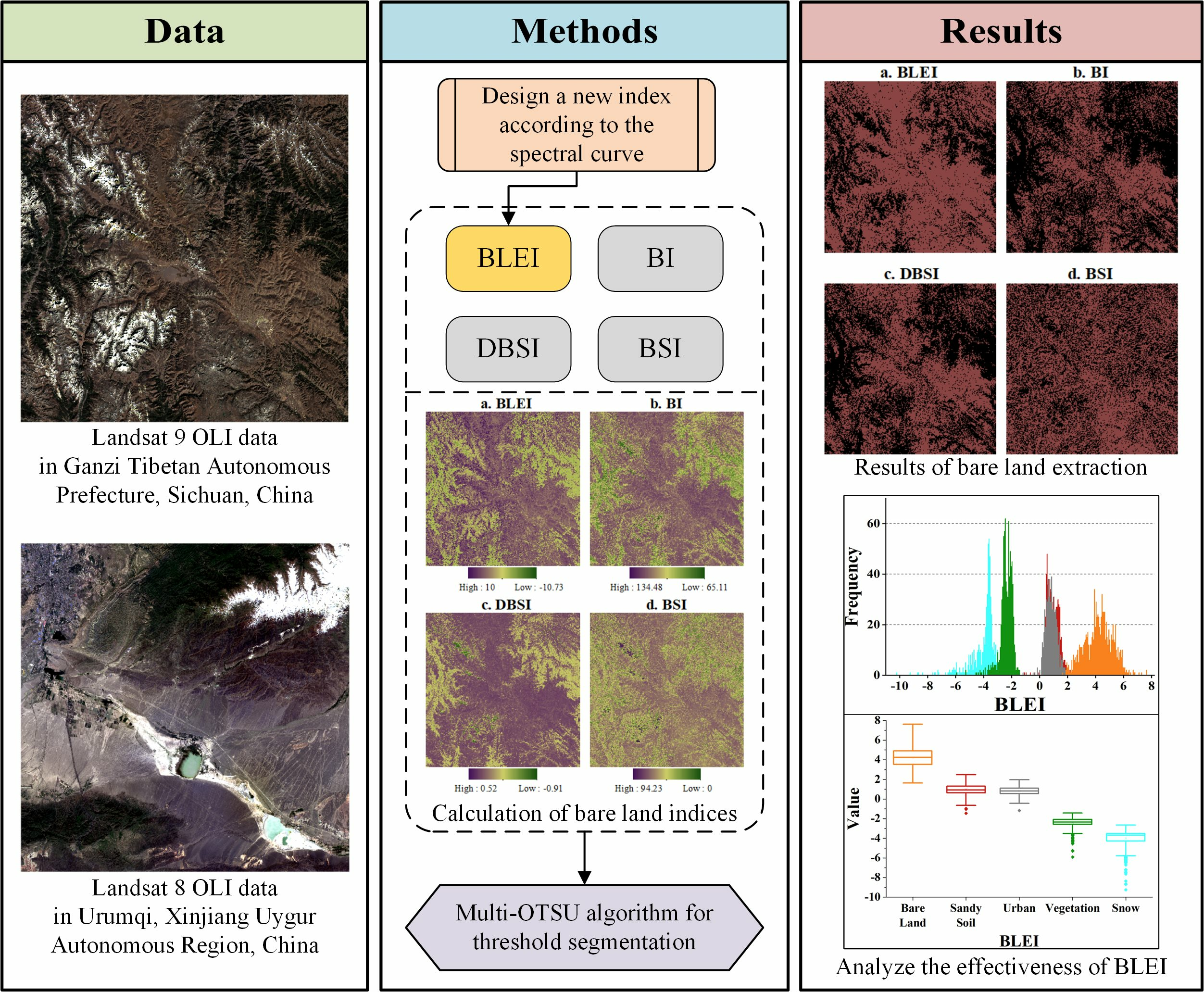
2. Study Area and Datasets

2.1. Study Area

The geographical region in the study is situated in the southwestern Ganzi Tibetan Autonomous Prefecture in western Sichuan Province, China (Figure 1), with geographical coordinates ranging from 29°32′N to 30°57′N and 98°57′E to 100°49′E. It predominantly covers Batang County and Litang County, including the urban portion of Litang County. Its altitude ranges from 2500 to 4500 m, with plateaus and mountains. As for climate, the study area falls within the plateau climatic zone, with the presence of snow cover and minimal water bodies. Under unique geological conditions and against the backdrop of global climate change, soil desertification has emerged in this region [56].

In addition, to validate the applicability of the proposed index, this study also selects Urumqi City in Xinjiang Province, northwestern China as another case (Figure 1). It mainly covers Urumqi County, Tianshan District, and includes urban areas belonging to a continental arid climate in the temperate zone, characterized by snowy mountains, sandy soil, and water body.

2.2. Data

The remote sensing satellites Landsat 8 and Landsat 9, collaboratively launched by the National Aeronautics and Space Administration (NASA) and the United States Geological Survey (USGS), successfully ascended into orbit in February 2013 and September 2021, respectively. Equipped with advanced remote sensing sensors, including the Operational Land Imager (OLI) and Thermal Infrared Sensor (TIRS), Landsat 8 and Landsat 9 enable high-resolution monitoring of the Earth’s surface [57]. The data obtained from these sophisticated sensors find extensive applications within the realms like agriculture, forestry, urban planning, and environmental monitoring, providing crucial information for scientific research, resource management, and environmental protection [58,59].

To conduct this study, we acquired Landsat 8 OLI and Landsat 9 OLI image data, comprising seven spectral bands, namely Coastal (0.43–0.45 μm), Blue (0.45–0.51 μm), Green (0.53–0.59 μm), Red (0.64–0.67 μm), Near Infrared (NIR, 0.85–0.88 μm), Short-wave Infrared1 (SWIR1, 1.57–1.65 μm), and Short-wave Infrared2 (SWIR2, 2.11–2.29 μm), with a spatial resolution of 30 m. These bands cover the spectral regions of visible light, near-infrared, and shortwave infrared, providing diversity and comprehensiveness for remote sensing analysis and serving as a robust data foundation for bare land-extraction research. As indicated in

Table 1. Remote sensing image data table in this study.

Satellite	Acquisition Date	Strip Number	Cloud Coverage	Spatial Resolution
Landsat 9 OLI	20 November 2022	132,039	0.86%	30 m
Landsat 8 OLI	13 June 2017	142,030	1.45%	30 m

, the Landsat 9 OLI image was acquired from the website https://earthexplorer.usgs.gov/ (accessed on 10 December 2023) with the acquisition date of 20 November 2022 and a cloud coverage of 0.86%, because the study area is covered with sparse vegetation, leading to a predominance of bare land in the remote sensing image in winter. To validate the effectiveness of the BLEI in various environments, we also acquired Landsat 8 OLI images of Urumqi City, captured on June 13, 2016, during the summer season, with a cloud cover of 1.45% (Table 1).

3. Methods

The technical flowchart of this study is illustrated in Figure 2. Initially, preprocessing steps such as radiometric correction and cutting are applied to the Landsat 8 OLI and Landsat 9 OLI images. Subsequently, to validate the effectiveness of the proposed Bare Land Extraction Index (BLEI), a comparative analysis is conducted against existing indices, including the BI, DBSI, and BSI. Then, the Multi-Otsu Thresholding (MOT) algorithm is employed to extract bare land. Finally, based on validation samples, quantitative analysis is performed using metrics such as the Spectral Discrimination Index (SDI), overall accuracy (OA), and kappa coefficient to comprehensively assess the effectiveness of BLEI in bare land extraction.

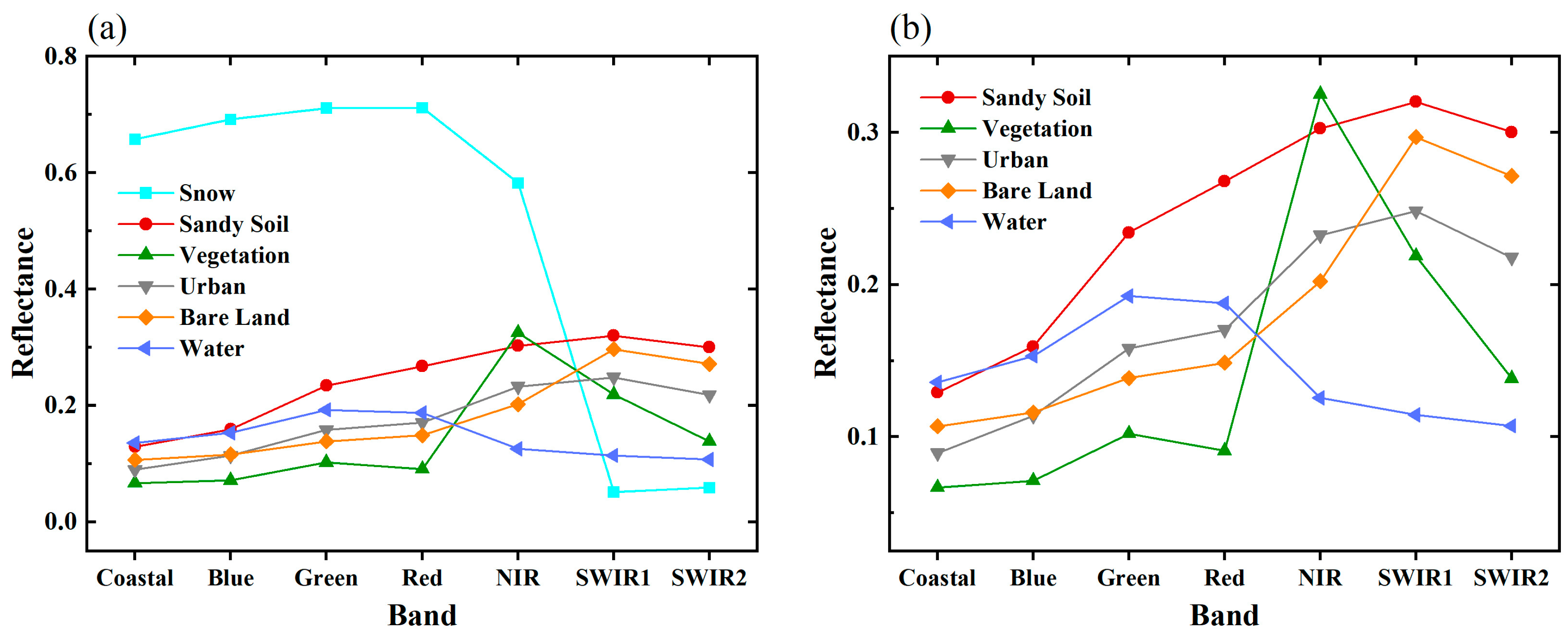
3.1. Development of the Bare Land Extraction Index (BLEI)

After radiometric calibration, atmospheric correction, and topographic correction to obtain surface true reflectance data, this study extracted several pure pixels representing six land cover types: snow, sandy soil, vegetation, urban areas, bare land, and water bodies. To delineate the spectral characteristics of each ground object type, the average reflectance values across all pixels within each category were computed for every spectral band. These average values were then utilized to generate corresponding spectral profiles for each land-cover type (Figure 3).

Upon analyzing the spectral reflectance profiles (Figure 3), we can observe that the difference in reflectance between the SWIR1 and Red bands for bare land is significantly greater than the difference between the Red and Blue bands. On the basis of this characteristic, Equation (1) is formulated, ensuring that the K values for sandy soil and urban areas are positive but lower than that of bare land, facilitating differentiation. However, we also note that the spectral characteristics of snow and vegetation similarly conform to the aforementioned spectral features of bare land, resulting in high value of K. Therefore, we proposed specific constraints M with Equation (2). Generally, the M values are negative for snow, vegetation, and water bodies, while positive for other land features. Additionally, to address situations where the Red and Blue band reflectance differences for certain pixels (e.g., snow, vegetation, and a few bare land pixels) are small, potentially causing excessively high K values (reaching hundreds or thousands), Equation (3) is designed to compress the K values so that they are closer to 0 for subsequent analysis. Following the application of Equations (1)–(3), the K values, as well as BLEI values, are negative for snow, vegetation, and water bodies, while positive for bare land, sandy soil, and urban areas.

$$K=\left\{\begin{array}{c}-\left|\frac{SWIR1-Red}{Red-Blue}\right|, M<0\\ \left|\frac{SWIR1-Red}{Red-Blue}\right|, M\ge 0\end{array}\right.$$

(1)

$$M=SWIR1-NIR$$

(2)

$$BLEI=\left\{\begin{array}{cc}\hfill -\ln \left(\left|K\right|+1\right),& K<0\hfill \\ \hfill K,& 0\le K<10\hfill \\ \hfill 10,& K\ge 10\hfill \end{array}\right.$$

(3)

where, Blue, Red, NIR, and SWIR1 are the Blue Band 2, Red Band 4, Near-Infrared Band 5, and Shortwave Infrared Band 6 on the Landsat 8 OLI and Landsat 9 OLI images, respectively.

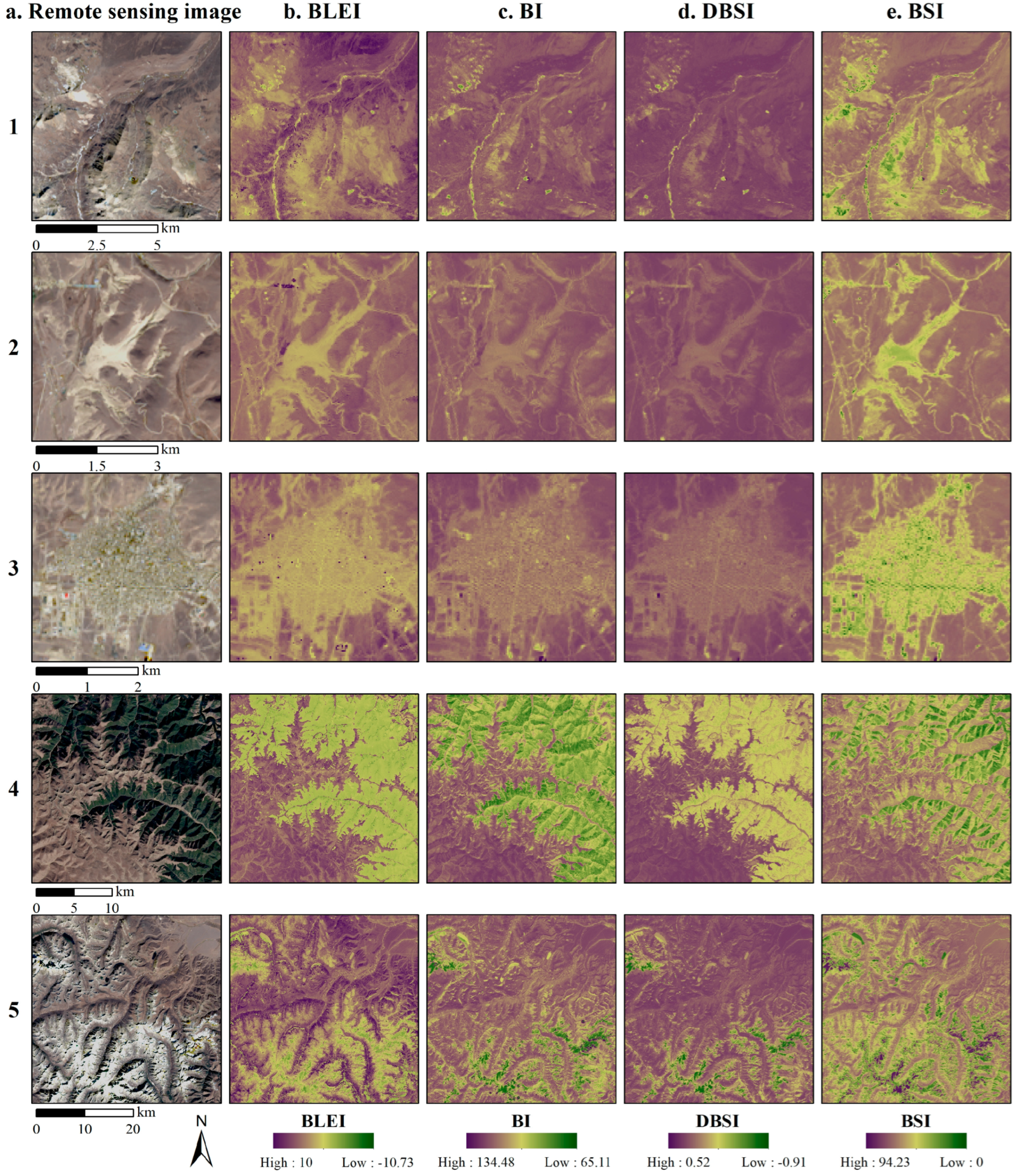
3.2. Comparison with Other Related Remote Sensing Indices

To evaluate the effectiveness of BLEI in bare land extraction, this study conducted experimental comparisons with three soil indices, namely BI [39], DBSI [44], and BSI [40]. Their respective calculation formulas are as follows:

$$BI=\frac{\left(SWIR1+Red\right)-\left(NIR+Blue\right)}{\left(SWIR1+Red\right)+\left(NIR+Blue\right)}\ast 100+100$$

(4)

$$DBSI=\frac{SWIR1-Green}{SWIR1+Green}-NDVI$$

(5)

$$NDVI=\frac{NIR-Red}{NIR+Red}$$

(6)

$$BSI=100\times \sqrt{\frac{\left|SWIR2-Green\right|}{SWIR2+Green}}$$

(7)

where, Blue, Green, Red, NIR, SWIR1, and SWIR2 represent Blue Band 2, Green Band 3, Red Band 4, Near-Infrared Band 5, Shortwave Infrared Band 6, and Shortwave Infrared Band 7 on the Landsat 8 OLI and Landsat 9 OLI images, respectively.

3.3. Identification of Bare Land Using the Multi-Otsu Thresholding Algorithm

In the common scenarios, spectral index images of single bands or multispectral images can be classified using supervised or unsupervised classification algorithms. However, for the identification of specific and singular land-cover types, threshold segmentation algorithms are considered the most straightforward and simplest method [60,61]. In this study, due to the presence of more than two ground object types within this analyzed region, exhibiting multiple peaks on the frequency distribution histogram, traditional binary threshold segmentation algorithms struggle to cope with images displaying multiple histogram peaks, resulting in suboptimal extraction performance [62]. To enhance the accuracy of bare land identification, we use the Multi-Otsu Thresholding (MOT) algorithm to determine the bare land thresholds for each spectral index instead of conventional ones such as the Otsu algorithm [63].

The MOT segmentation algorithm, an extension of the traditional Otsu method, aims to divide the image into n categories whose core idea involves selecting the optimal threshold set T = {T₁, T₂, …, T_n−1} based on minimizing intra-class variance or maximizing inter-class variance [64]. By gradually changing the threshold set, the algorithm decreases the pixel variance within each category while increasing the differences between different categories. This optimization process involves objective functions such as probability distribution and variance for each category. Ultimately, by identifying the threshold combination that maximizes inter-class variance or minimizes intra-class variance, effective segmentation of the image is achieved. In multi-class scenarios, this method provides a finer grayscale segmentation, offering more detailed information for image analysis and processing [65]. In this study, the MOT segmentation algorithm proves more effective in handling complex histograms with multiple peaks. By simultaneously considering multiple thresholds, it adapts more flexibly to the complex arrangement of ground object types, enhancing adaptability and accuracy in multi-class segmentation. After computing the BLEI, BI, DBSI, and BSI, this study utilizes the MOT algorithm to obtain appropriate thresholds for classifying the image into bare land and non-bare land categories.

3.4. Performance and Accuracy

To examine the discriminability or dissimilarity of BLEI in separating bare land from other land features, this study employs SDI for quantitative measurement [66]. SDI quantifies the level of distinction between two land-cover types by calculating the ratio of the difference between the mean values of the indices for the two classes to the sum of their standard deviations (Equation (8)). A higher SDI value signifies a greater separability and larger differences between the two land-cover types, making them easier to be separated [16]. Conversely, a smaller SDI value indicates a higher level of histogram confusion and overlap, indicating lower separability and greater difficulty in differentiation. Typically, SDI < 1 suggests poor separability between the two land-cover types, making discrimination more difficult [67]. Through the quantitative calculation of SDI values, a comprehensive assessment of BLEI’s effectiveness in bare land extraction is achieved, providing a quantitative foundation for further analysis.

$$SDI=\frac{\left|m_1-m_2\right|}{s_1+s_2}$$

(8)

where m₁ and m₂ are the mean values of indices for ground object types 1 and 2, while s₁ and s₂ are the standard deviations of indices for ground object types 1 and 2.

In addition to SDI, this study utilizes five accuracy metrics—OA, kappa coefficient, recall, precision, and F1-score—to assess BLEI’s performance in bare land extraction. In this study, Recall represents the proportion of pixels correctly identified as bare land relative to all bare land pixels in the validation set (producer’s accuracy), while precision represents the proportion of pixels correctly identified as bare land relative to all pixels identified as bare land (user’s accuracy) [68]. The F1-score is the harmonic mean of recall and precision, serving as a metric for assessing the accuracy of binary classification results [69]. A higher F1 value indicates more effective performance. The calculation methods for these five metrics are as follows:

$$OA=\frac{TP+TN}{FN+TP+FP+TN}$$

(9)

$$P=\frac{\left(FN+TP\right)\times \left(FP+TP\right)+\left(FP+TN\right)\times \left(FN+TN\right)}{{\left(FN+TP+FP+TN\right)}^2}$$

(10)

$$Kappa=\frac{OA-P}{1-P}$$

(11)

$$Recall=\frac{TP}{FN+TP}$$

(12)

$$Precision=\frac{TP}{FP+TP}$$

(13)

$$\mathrm{F}1=\frac{2·Recall·Precision}{Recall+Precision}$$

(14)

where, in this study, TP (true positives) is the number of bare land pixels in the validation set correctly predicted as bare land, TN (true negatives) represents the count of non-bare land pixels in the validation set correctly predicted as non-bare land, FN (false negatives) denotes the number of bare land pixels erroneously predicted as non-bare land pixels (missed classifications), and FP (false positives) represents the count of non-bare land pixels erroneously identified as bare land pixels (misclassifications).

4. Results

From Landsat 9 OLI image, we selected 916 bare land pixels, 626 sandy-soil pixels, 775 vegetation pixels, 576 urban pixels, and 579 snow pixels, while from Landsat 8 OLI image, we selected 485 bare land pixels, 374 sandy-soil pixels, 332 vegetation pixels, 309 urban pixels, 328 snow pixels, and 324 water pixels as validation samples for the study areas. Considering the limited water distribution in the study area in Ganzi Tibetan Autonomous Prefecture, water bodies were excluded from subsequent analyses for they are easily distinguishable with negative BLEI values as shown in Section 3.1. The calculated results of four bare land indices, BLEI, BI, DBSI, and BSI, are shown in Figure 4. Detailed comparisons of the extracted bare land images using the MOT algorithm are presented in Figure 5. To comprehensively assess the separability and dissimilarity of different indices for bare land and other land features, boxplots and frequency distribution histograms (Figure 6 and Figure 7) were generated, and SDI values between bare land and other five ground object types (sandy soil, urban areas, vegetation, snow, and water) were computed (

Table 2. Comparison of spectral discrimination index (SDI) for different indices (BLEI, BI, DBSI, and BSI) between bare land and other features.

Study Area	SDI	BLEI	BI	DBSI	BSI
Ganzi Tibetan	Bare land–sandy soil	2.27	0.78	1.03	1.33
	Bare land–urban	2.46	1.30	2.04	1.66
	Bare land–vegetation	4.52	3.03	3.87	1.54
	Bare land–snow	4.29	12.22	17.49	3.53
Urumqi	Bare land–sandy soil	1.31	0.56	0.28	0.35
	Bare land–urban	2.90	2.32	2.26	0.64
	Bare land–vegetation	4.94	4.68	5.33	2.87
	Bare land–snow	5.09	7.18	7.32	6.32
	Bare land–water	4.83	1.82	2.62	3.02

). Additionally, we examined the bare land thresholds and extraction accuracy metrics for different indices (

Table 3. Bare land-extraction precision comparison among different indices (BLEI, BI, DBSI, and BSI).

Study Area	Value	BLEI	BI	DBSI	BSI
Ganzi Tibetan	Threshold	2.44	116.55	0.21	51.74~72.77
	OA	98.91%	90.52%	93.26%	85.60%
	Kappa	0.97	0.75	0.83	0.65
	Recall	96.18%	80.79%	88.10%	84.28%
	Precision	99.66%	82.87%	86.59%	68.44%
	F1	97.89%	81.81%	87.34%	75.54%
Urumqi	Threshold	1.26	107.66~112.87	0.075~0.17	40.23~47.55
	OA	98.18%	88.74%	82.41%	78.97%
	Kappa	0.95	0.68	0.54	0.44
	Recall	93.00%	74.02%	74.64%	63.09%
	Precision	98.90%	75.58%	58.67%	52.85%
	F1	95.90%	74.79%	65.70%	57.52%

) to validate the effectiveness of BLEI in bare land extraction.

4.1. The Effectiveness of BLEI

Based on observations of Figure 4b, Figure 6a and Figure 7a, we can see that the BLEI values of bare land (greater than 1.6 in Ganzi and greater than 1.0 in Urumqi) appear as light purple or purple on the images, indicating positive values higher than other land features. In contrast, the BLEI values of sandy soil and urban areas (approximately −1~2 in Ganzi and −2~1 in Urumqi) are lower than those for bare land, appearing yellow and yellow-green on the images. Vegetation and snow exhibit negative BLEI values, primarily in shades of green and dark green. Detailed analysis of the bare land-extraction results after threshold segmentation (Figure 5) indicates that compared to the other indices (BI, DBSI, and BSI), BLEI can separate bare land from sandy soil, urban areas, vegetation, and snow (Figure 5b) more effectively. Furthermore, it accurately identifies some land covered with rocks and gravel to a certain extent as bare land (Figure 5(4)), further demonstrating the satisfactory effectiveness of BLEI in bare land extraction.

Additionally, quantitative analysis of the bare land index further validates the effectiveness of BLEI in bare land extraction (Table 2 and Table 3). As shown in Table 2, the SDI values of BLEI between bare land and other land features (sandy soil, urban areas, vegetation, and snow) in Ganzi are 2.27, 2.46, 4.52, and 4.29, respectively. All SDI values exceed 2 and generally surpass those of other indices (although the SDI value for bare land–snow is lower than those for BI and DBSI, bare land and snow can still be effectively distinguished), indicating a significant level of separability between bare land and other land features. The situation in the Urumqi study area is similar in nature, with SDI values between bare land and sandy soil, as well as urban areas, being 1.31 and 2.90, respectively, both higher than other indices. Meanwhile, BLEI exhibits high accuracy in bare land extraction (Table 3), with OA, kappa coefficient, recall, precision, and F1-score for both study areas exceeding 98%, 0.95, 93%, 98%, and 95%, respectively, all surpassing BI, DBSI, and BSI.

4.2. Comparisons of BLEI with Other Spectral Indices

4.2.1. BI

Analyzing Figure 4c, Figure 6b(1) and Figure 7b(1), in Ganzi, the BI values for bare land are the highest (greater than 110), while the BI values for sandy soil and urban areas are roughly in the range of 100 to 120. Vegetation has BI values between 75 and 100, while snow has the smallest BI values, less than 75. The SDI values for bare land–snow and bare land–vegetation are exceptionally high, reaching 12.22 and 3.03, respectively (Table 2). Referring to Figure 5c(3,4), this indicates that BI effectively separates bare land from these land-cover types. However, the SDI values for bare land–urban and bare land–sandy soil in Ganzi are relatively low (1.30 and 0.78), and the SDI value for bare land–sandy soil in Urumqi is also low (0.56), both lower than BLEI (Table 2). This suggests a certain degree of overlap and confusion between urban areas, sandy soil, and bare land (Figure 6b and Figure 7b), leading BI to misclassify some sandy soil and urban areas as bare land (Figure 5c(1,2)). Additionally, compared to BLEI, BI fails to accurately identify soil covered with gravel and rocks as bare land (Figure 5c(4)). As shown in Table 3, in Ganzi, BI’s OA, kappa coefficient, and F1-score are 90.52%, 0.75, and 81.81%, respectively, while in Urumqi, they are 88.74%, 0.68, and 74.79%, respectively, indicating lower accuracy in bare land extraction compared to BLEI.

4.2.2. DBSI

As shown in Figure 4d, Figure 6c(1) and Figure 7c(1), in Ganzi, for the DBSI, bare land values are the highest (greater than 0.1), followed by sandy soil (0~0.3), urban areas (0~0.2), vegetation (−0.3~0), and snow (less than −0.7). According to Table 2, the SDI values for bare land–urban in Ganzi and Urumqi are 2.04 and 2.26, respectively, slightly lower than BLEI, but they still exhibit good separation (Figure 5d(2,3)). However, from Figure 6c and Figure 7c, we can observe that there is a certain degree of overlap between bare land and sandy soil, as confirmed by the SDI value for bare land–sandy soil being relatively low (1.03 in Ganzi and 0.28 in Urumqi) in Table 2. This overlap results in some confusion between bare land and sandy soil during the bare land-extraction process with DBSI, as illustrated in Figure 5d(1), where sandy soil is incorrectly identified as bare land. Moreover, similar to BI, DBSI also fails to accurately extract bare land covered with gravel and rocks (Figure 5d(4)). In terms of mapping accuracy (Table 3), in Ganzi, DBSI’s OA, kappa coefficient, and F1-score are 93.26%, 0.83, and 87.34%, respectively, while in Urumqi, they are 82.41%, 0.54, and 65.70%, respectively, showing lower accuracy and potential in bare land extraction compared to BLEI.

4.2.3. BSI

Upon analyzing Figure 4e, Figure 6d(1) and Figure 7d(1), in Ganzi, it is evident that BSI values are highest for snow (greater than 80), followed by bare land (30~80), vegetation (10~60), sandy soil (20~60), and urban areas (20~60). For the BSI, it is necessary to establish upper and lower threshold values to extract bare land. Through Figure 6d and Figure 7d, it becomes apparent that there is a certain degree of confusion between bare land and the other three land features: sandy soil, urban areas, and vegetation. The SDI values for bare land with these three land cover types are relatively low (Table 2) and are all below BLEI both in Ganzi and Urumqi. This leads to challenges in accurately delineating the threshold for bare land in BSI. Consequently, the resulting bare land classification map (Figure 5e) using BSI exhibits numerous misclassifications and omissions. For instance, some sandy soil, urban areas, vegetation, and snow are incorrectly identified as bare land (Figure 5e(1–4)), and certain bare land areas are not accurately extracted (Figure 5e(4)). Furthermore, in Ganzi, BSI’s OA, kappa coefficient, and F1-score are 85.60%, 0.65, and 75.54%, respectively, while in Urumqi, they are 78.97%, 0.44, and 57.52%, respectively (Table 3), making it the least effective among the four indices in the field of bare land extraction.

5. Discussion

Taking Ganzi Prefecture and Urumqi as study areas, BLEI can more easily distinguish bare land from other land-cover types. Compared to the other three indices (BI, DBSI, and BSI), the high SDI values between bare land and other land features, particularly sandy soil and urban areas, indicate the efficacy of BLEI in accurately extracting bare land through threshold segmentation algorithms. In Urumqi, due to the arid climatic environment, the similarity in spectral characteristics between bare land and sandy soil increases. This results in a greater degree of confusion between bare land and sandy soil for all indices compared to Ganzi Prefecture, and the separability between them decreases (Figure 6 and Figure 7). But in contrast to the other three indices, BLEI still achieves excellent results in distinguishing between bare land and sandy soil. Furthermore, BLEI demonstrates strong capabilities in bare land extraction in both Ganzi Prefecture and Urumqi, which have different climatic environments, while the other three indices perform poorly in these two study areas (Table 2 and Table 3), suggesting that BLEI has significant potential in bare land extraction. Notably, BLEI, with its highest values for bare land, requires only a lower threshold, laying the foundation for fast and accurate extraction, whereas by contrast, BI, DBSI, and BSI require both upper- and lower-threshold values under certain environmental conditions (Table 3).

In the future, it may be worth considering the impact of certain special roofing materials found in urban areas to improve accuracy. For instance, in this study, blue roofs displaying higher BLEI values may lead to confusion with bare land. Additionally, BLEI’s reliance on visible, near-infrared, and shortwave infrared bands without the need for thermal infrared bands makes it applicable to most satellite remote sensing sensors [70]. Therefore, future research could consider utilizing remote sensing images from other satellites to validate the effectiveness of BLEI. Furthermore, without considering factors such as time costs and the quality of training samples, integrating this index with machine learning or deep learning technologies might potentially contribute to research fields related to land use and ecological environments.

6. Conclusions

This study uses Landsat 9 and Landsat 8 OLI images with four bands of Blue, Red, NIR, and SWIR1, to design the Bare Land Extraction Index (BLEI) to achieve rapid and accurate extraction of bare land from five distinct land cover types, sandy soil, urban areas, vegetation, snow, and water bodies, and investigates its effectiveness in two distinct climatic environments: Ganzi and Urumqi. Both qualitative and quantitative analyses indicate that the proposed BLEI outperforms BI, DBSI, and BSI in various aspects of bare land extraction. It is essential to highlight BLEI’s enhanced separability between bare land and sandy soil or urban areas. Particularly for sandy soil, where few bare land indices are available, BLEI proves valuable, especially in regions with severe soil desertification like western Sichuan and northwest China. Moreover, compared to some other indices, BLEI requires only a lower threshold for bare land extraction, making it more convenient and efficient. This suggests that BLEI holds significant applications for future studies focused on bare land analysis.

References

1. Zhang, M.; Huang, H.; Li, Z.; Hackman, K.O.; Liu, C.; Andriamiarisoa, R.L.; Ny Aina Nomenjanahary Raherivelo, T.; Li, Y.; Gong, P. Automatic High-Resolution Land Cover Production in Madagascar Using Sentinel-2 Time Series, Tile-Based Image Classification and Google Earth Engine. Remote Sens. 2020, 12, 3663. [Google Scholar] [CrossRef]
2. Yalew, S.; Mul, M.; Van Griensven, A.; Teferi, E.; Priess, J.; Schweitzer, C.; Van Der Zaag, P. Land-Use Change Modelling in the Upper Blue Nile Basin. Environments 2016, 3, 21. [Google Scholar] [CrossRef]
3. Mahmoud, S.H.; Alazba, A.A. Hydrological Response to Land Cover Changes and Human Activities in Arid Regions Using a Geographic Information System and Remote Sensing. PLoS ONE 2015, 10, e0125805. [Google Scholar] [CrossRef]
4. Peng, K.; Jiang, W.; Ling, Z.; Hou, P.; Deng, Y. Evaluating the Potential Impacts of Land Use Changes on Ecosystem Service Value under Multiple Scenarios in Support of SDG Reporting: A Case Study of the Wuhan Urban Agglomeration. J. Clean. Prod. 2021, 307, 127321. [Google Scholar] [CrossRef]
5. Wang, H.; Zhang, Y.; Tsou, J.; Li, Y. Surface Urban Heat Island Analysis of Shanghai (China) Based on the Change of Land Use and Land Cover. Sustainability 2017, 9, 1538. [Google Scholar] [CrossRef]
6. Mertes, C.M.; Schneider, A.; Sulla-Menashe, D.; Tatem, A.J.; Tan, B. Detecting Change in Urban Areas at Continental Scales with MODIS Data. Remote Sens. Environ. 2015, 158, 331–347. [Google Scholar] [CrossRef]
7. Foley, J.A.; DeFries, R.; Asner, G.P.; Barford, C.; Bonan, G.; Carpenter, S.R.; Chapin, F.S.; Coe, M.T.; Daily, G.C.; Gibbs, H.K.; et al. Global Consequences of Land Use. Science 2005, 309, 570–574. [Google Scholar] [CrossRef] [PubMed]
8. Kuenzer, C.; Heimhuber, V.; Huth, J.; Dech, S. Remote Sensing for the Quantification of Land Surface Dynamics in Large River Delta Regions—A Review. Remote Sens. 2019, 11, 1985. [Google Scholar] [CrossRef]
9. Fikadu, G.; Olika, G. Impact of Land Use Land Cover Change Using Remote Sensing with Integration of Socio-Economic Data on Rural Livelihoods in the Nashe Watershed, Ethiopia. Heliyon 2023, 9, e13746. [Google Scholar] [CrossRef]
10. Nguyen, C.T.; Chidthaisong, A.; Kieu Diem, P.; Huo, L.-Z. A Modified Bare Soil Index to Identify Bare Land Features during Agricultural Fallow-Period in Southeast Asia Using Landsat 8. Land 2021, 10, 231. [Google Scholar] [CrossRef]
11. Chen, Y.; Liu, A. Spatial and Temporal Variations of Bare Land in Beijing, China: A 30-Year Analysis. In Patterns and Mechanisms of Climate, Paleoclimate and Paleoenvironmental Changes from Low-Latitude Regions; Zhang, Z., Khélifi, N., Mezghani, A., Heggy, E., Eds.; Advances in Science, Technology & Innovation; Springer International Publishing: Cham, Switzerland, 2019; pp. 159–162. ISBN 978-3-030-01598-5. [Google Scholar]
12. Tesfaye, A.T.; Defersha, D.T. Contribution to the Land Suitability Analysis for Potential Surface Irrigation Development Using Remote Sensing and GIS-MCE of the Soroka Watershed, Northwestern Ethiopia. Sustain. Water Resour. Manag. 2024, 10, 51. [Google Scholar] [CrossRef]
13. Liu, Y.; Wu, J.; Huang, T.; Nie, W.; Jia, Z.; Gu, Y.; Ma, X. Study on the Relationship between Regional Soil Desertification and Salinization and Groundwater Based on Remote Sensing Inversion: A Case Study of the Windy Beach Area in Northern Shaanxi. Sci. Total Environ. 2024, 912, 168854. [Google Scholar] [CrossRef]
14. Sorenson, P.T.; Kiss, J.; Bedard-Haughn, A.K.; Shirtliffe, S. Multi-Horizon Predictive Soil Mapping of Historical Soil Properties Using Remote Sensing Imagery. Remote Sens. 2022, 14, 5803. [Google Scholar] [CrossRef]
15. Liu, Y.; Lu, C.; Mao, J.; Pang, J.; Liu, Z.; Hou, M. Comprehensive Evaluation of the Importance of Ecological Land in Arid Hilly Cities in Northwest China: A Case Study of the Core Urban Area of Lanzhou. Land 2021, 10, 942. [Google Scholar] [CrossRef]
16. Liu, Y.; Meng, Q.; Zhang, L.; Wu, C. NDBSI: A Normalized Difference Bare Soil Index for Remote Sensing to Improve Bare Soil Mapping Accuracy in Urban and Rural Areas. Catena 2022, 214, 106265. [Google Scholar] [CrossRef]
17. Enoguanbhor, E.; Gollnow, F.; Nielsen, J.; Lakes, T.; Walker, B. Land Cover Change in the Abuja City-Region, Nigeria: Integrating GIS and Remotely Sensed Data to Support Land Use Planning. Sustainability 2019, 11, 1313. [Google Scholar] [CrossRef]
18. Zhu, Z.; Cao, H.; Yang, J.; Shang, H.; Ma, J. Ecological Environment Quality Assessment and Spatial Autocorrelation of Northern Shaanxi Mining Area in China Based-on Improved Remote Sensing Ecological Index. Front. Environ. Sci. 2024, 12, 1325516. [Google Scholar] [CrossRef]
19. Zou, Q.; Yu, W.; Bao, Z. A Blockchain Solution for Remote Sensing Data Management Model. Appl. Sci. 2023, 13, 9609. [Google Scholar] [CrossRef]
20. Li, H.; Jiang, H.; Gu, X.; Peng, J.; Li, W.; Hong, L.; Tao, C. CLRS: Continual Learning Benchmark for Remote Sensing Image Scene Classification. Sensors 2020, 20, 1226. [Google Scholar] [CrossRef]
21. Qi, L.; Li, J.; Wang, Y.; Gao, X. Urban Observation: Integration of Remote Sensing and Social Media Data. IEEE J. Sel. Top. Appl. Earth Obs. Remote Sens. 2019, 12, 4252–4264. [Google Scholar] [CrossRef]
22. Chi, J.; Lee, H.; Hong, S.G.; Kim, H.-C. Spectral Characteristics of the Antarctic Vegetation: A Case Study of Barton Peninsula. Remote Sens. 2021, 13, 2470. [Google Scholar] [CrossRef]
23. Chen, Y.; He, C.; Guo, W.; Zheng, S.; Wu, B. Mapping Urban Functional Areas Using Multisource Remote Sensing Images and Open Big Data. IEEE J. Sel. Top. Appl. Earth Obs. Remote Sens. 2023, 16, 7919–7931. [Google Scholar] [CrossRef]
24. Xie, X.; Ye, L.; Kang, X.; Yan, L.; Zeng, L. Land Use Classification Using Improved U-Net in Remote Sensing Images of Urban and Rural Planning Monitoring. Sci. Program. 2022, 2022, 3125414. [Google Scholar] [CrossRef]
25. Cui, W.; Zheng, Z.; Zhou, Q.; Huang, J.; Yuan, Y. Application of a Parallel Spectral–Spatial Convolution Neural Network in Object-Oriented Remote Sensing Land Use Classification. Remote Sens. Lett. 2018, 9, 334–342. [Google Scholar] [CrossRef]
26. Ali, U.; Esau, T.J.; Farooque, A.A.; Zaman, Q.U.; Abbas, F.; Bilodeau, M.F. Limiting the Collection of Ground Truth Data for Land Use and Land Cover Maps with Machine Learning Algorithms. ISPRS Int. J. Geo-Inf. 2022, 11, 333. [Google Scholar] [CrossRef]
27. Kirsten, T.; Hoffman, M.T.; Bell, W.D.; Visser, V. A Regional, Remote Sensing-Based Approach to Mapping Land Degradation in the Little Karoo, South Africa. J. Arid Environ. 2023, 219, 105066. [Google Scholar] [CrossRef]
28. Ramadhani, F.; Pullanagari, R.; Kereszturi, G.; Procter, J. Mapping of Rice Growth Phases and Bare Land Using Landsat-8 OLI with Machine Learning. Int. J. Remote Sens. 2020, 41, 8428–8452. [Google Scholar] [CrossRef]
29. Shi, Y.; Qi, Z.; Liu, X.; Niu, N.; Zhang, H. Urban Land Use and Land Cover Classification Using Multisource Remote Sensing Images and Social Media Data. Remote Sens. 2019, 11, 2719. [Google Scholar] [CrossRef]
30. He, C.; Liu, Y.; Wang, D.; Liu, S.; Yu, L.; Ren, Y. Automatic Extraction of Bare Soil Land from High-Resolution Remote Sensing Images Based on Semantic Segmentation with Deep Learning. Remote Sens. 2023, 15, 1646. [Google Scholar] [CrossRef]
31. Liu, L.; Tang, X.; Gan, Y.; You, S.; Luo, Z.; Du, L.; He, Y. Research on Optimization of Processing Parcels of New Bare Land Based on Remote Sensing Image Change Detection. Remote Sens. 2022, 15, 217. [Google Scholar] [CrossRef]
32. Xu, B. Improved Convolutional Neural Network in Remote Sensing Image Classification. Neural Comput. Appl. 2021, 33, 8169–8180. [Google Scholar] [CrossRef]
33. Tu, B.; Zhou, C.; Kuang, W.; Chen, S.; Plaza, A. Multiattribute Sample Learning for Hyperspectral Image Classification Using Hierarchical Peak Attribute Propagation. IEEE Trans. Instrum. Meas. 2022, 71, 1–17. [Google Scholar] [CrossRef]
34. Estoque, R.C.; Murayama, Y. Classification and Change Detection of Built-up Lands from Landsat-7 ETM+ and Landsat-8 OLI/TIRS Imageries: A Comparative Assessment of Various Spectral Indices. Ecol. Indic. 2015, 56, 205–217. [Google Scholar] [CrossRef]
35. Deng, C.; Wu, C. BCI: A Biophysical Composition Index for Remote Sensing of Urban Environments. Remote Sens. Environ. 2012, 127, 247–259. [Google Scholar] [CrossRef]
36. Becker, F.; Choudhury, B.J. Relative Sensitivity of Normalized Difference Vegetation Index (NDVI) and Microwave Polarization Difference Index (MPDI) for Vegetation and Desertification Monitoring. Remote Sens. Environ. 1988, 24, 297–311. [Google Scholar] [CrossRef]
37. Zha, Y.; Gao, J.; Ni, S. Use of Normalized Difference Built-up Index in Automatically Mapping Urban Areas from TM Imagery. Int. J. Remote Sens. 2003, 24, 583–594. [Google Scholar] [CrossRef]
38. McFeeters, S.K. The Use of the Normalized Difference Water Index (NDWI) in the Delineation of Open Water Features. Int. J. Remote Sens. 1996, 17, 1425–1432. [Google Scholar] [CrossRef]
39. Rikimaru, A.; Roy, P.; Miyatake, S. Tropical Forest Cover Density Mapping. Trop. Ecol. 2002, 43, 39–47. [Google Scholar]
40. Wentzel, K. Determination of the Overall Soil Erosion Potential in the Nsikazi District (Mpumalanga Province, South Africa) Using Remote Sensing and GIS. Can. J. Remote Sens. 2002, 28, 322–327. [Google Scholar] [CrossRef]
41. Diek, S.; Fornallaz, F.; Schaepman, M.E.; De Jong, R. Barest Pixel Composite for Agricultural Areas Using Landsat Time Series. Remote Sens. 2017, 9, 1245. [Google Scholar] [CrossRef]
42. Deng, Y.; Wu, C.; Li, M.; Chen, R. RNDSI: A Ratio Normalized Difference Soil Index for Remote Sensing of Urban/Suburban Environments. Int. J. Appl. Earth Obs. Geoinf. 2015, 39, 40–48. [Google Scholar] [CrossRef]
43. As-syakur, A.R.; Adnyana, I.W.S.; Arthana, I.W.; Nuarsa, I.W. Enhanced Built-Up and Bareness Index (EBBI) for Mapping Built-Up and Bare Land in an Urban Area. Remote Sens. 2012, 4, 2957–2970. [Google Scholar] [CrossRef]
44. Rasul, A.; Balzter, H.; Ibrahim, G.; Hameed, H.; Wheeler, J.; Adamu, B.; Ibrahim, S.; Najmaddin, P. Applying Built-Up and Bare-Soil Indices from Landsat 8 to Cities in Dry Climates. Land 2018, 7, 81. [Google Scholar] [CrossRef]
45. Qi, L.; Shi, P.; Dvorakova, K.; Van Oost, K.; Sun, Q.; Yu, H.; Van Wesemael, B. Detection of Soil Erosion Hotspots in the Croplands of a Typical Black Soil Region in Northeast China: Insights from Sentinel-2 Multispectral Remote Sensing. Remote Sens. 2023, 15, 1402. [Google Scholar] [CrossRef]
46. Rukhovich, D.I.; Koroleva, P.V.; Rukhovich, A.D.; Komissarov, M.A. Informativeness of the Long-Term Average Spectral Characteristics of the Bare Soil Surface for the Detection of Soil Cover Degradation with the Neural Network Filtering of Remote Sensing Data. Remote Sens. 2022, 15, 124. [Google Scholar] [CrossRef]
47. Li, H.; Wang, C.; Zhong, C.; Su, A.; Xiong, C.; Wang, J.; Liu, J. Mapping Urban Bare Land Automatically from Landsat Imagery with a Simple Index. Remote Sens. 2017, 9, 249. [Google Scholar] [CrossRef]
48. Lõhmus, K.; Oja, T.; Lasn, R. Specific Root Area: A Soil Characteristic. Plant Soil 1989, 119, 245–249. [Google Scholar] [CrossRef]
49. Barnes, E.M.; Sudduth, K.A.; Hummel, J.W.; Lesch, S.M.; Corwin, D.L.; Yang, C.; Daughtry, C.S.T.; Bausch, W.C. Remote- and Ground-Based Sensor Techniques to Map Soil Properties. Photogramm. Eng. Remote Sens. 2003, 69, 619–630. [Google Scholar] [CrossRef]
50. Wang, W.; Yao, X.; Ji, M. Integrating Seasonal Optical and Thermal Infrared Spectra to Characterize Urban Impervious Surfaces with Extreme Spectral Complexity: A Shanghai Case Study. J. Appl. Remote Sens. 2016, 10, 016018. [Google Scholar] [CrossRef]
51. Ben-Dor, E. Quantitative Remote Sensing of Soil Properties. In Advances in Agronomy; Academic Press: Cambridge, MA, USA, 2002; Volume 75, pp. 173–243. [Google Scholar]
52. Wu, C.; Murray, A.T. Estimating Impervious Surface Distribution by Spectral Mixture Analysis. Remote Sens. Environ. 2003, 84, 493–505. [Google Scholar] [CrossRef]
53. Roberts, D.A.; Quattrochi, D.A.; Hulley, G.C.; Hook, S.J.; Green, R.O. Synergies between VSWIR and TIR Data for the Urban Environment: An Evaluation of the Potential for the Hyperspectral Infrared Imager (HyspIRI) Decadal Survey Mission. Remote Sens. Environ. 2012, 117, 83–101. [Google Scholar] [CrossRef]
54. Chen, A.; Yang, X.; Guo, J.; Xing, X.; Yang, D.; Xu, B. Synthesized Remote Sensing-Based Desertification Index Reveals Ecological Restoration and Its Driving Forces in the Northern Sand-Prevention Belt of China. Ecol. Indic. 2021, 131, 108230. [Google Scholar] [CrossRef]
55. Wu, S.; Liu, Y.; Liu, S.; Wang, D.; Yu, L.; Ren, Y. Change Detection Enhanced by Spatial-Temporal Association for Bare Soil Land Using Remote Sensing Images. IEEE J. Sel. Top. Appl. Earth Obs. Remote Sens. 2024, 17, 150–161. [Google Scholar] [CrossRef]
56. Tu, M.; Lu, H.; Shang, M. Monitoring Grassland Desertification in Zoige County Using Landsat and UAV Image. Pol. J. Environ. Stud. 2021, 30, 5789–5799. [Google Scholar] [CrossRef]
57. Sun, Y.; Wang, B.; Teng, S.; Liu, B.; Zhang, Z.; Li, Y. Continuity of Top-of-Atmosphere, Surface, and Nadir BRDF-Adjusted Reflectance and NDVI between Landsat-8 and Landsat-9 OLI over China Landscape. Remote Sens. 2023, 15, 4948. [Google Scholar] [CrossRef]
58. Masek, J.G.; Wulder, M.A.; Markham, B.; McCorkel, J.; Crawford, C.J.; Storey, J.; Jenstrom, D.T. Landsat 9: Empowering Open Science and Applications through Continuity. Remote Sens. Environ. 2020, 248, 111968. [Google Scholar] [CrossRef]
59. Singh, R.; Saritha, V.; Pande, C.B. Monitoring of Wetland Turbidity Using Multi-Temporal Landsat-8 and Landsat-9 Satellite Imagery in the Bisalpur Wetland, Rajasthan, India. Environ. Res. 2024, 241, 117638. [Google Scholar] [CrossRef]
60. Mohd, O.; Suryanna, N.; Sahib Sahibuddin, S.; Faizal Abdollah, M.; Rahayu Selamat, S. Thresholding and Fuzzy Rule-Based Classification Approaches in Handling Mangrove Forest Mixed Pixel Problems Associated with in QuickBird Remote Sensing Image Analysis. Int. J. Agric. For. 2012, 2, 300–306. [Google Scholar] [CrossRef]
61. Mzid, N.; Pignatti, S.; Huang, W.; Casa, R. An Analysis of Bare Soil Occurrence in Arable Croplands for Remote Sensing Topsoil Applications. Remote Sens. 2021, 13, 474. [Google Scholar] [CrossRef]
62. Otsu, N. A Threshold Selection Method from Gray-Level Histograms. IEEE Trans. Syst. Man Cybern. 1979, 9, 62–66. [Google Scholar] [CrossRef]
63. Huang, D.-Y.; Wang, C.-H. Optimal Multi-Level Thresholding Using a Two-Stage Otsu Optimization Approach. Pattern Recognit. Lett. 2009, 30, 275–284. [Google Scholar] [CrossRef]
64. Zahara, E.; Fan, S.-K.S.; Tsai, D.-M. Optimal Multi-Thresholding Using a Hybrid Optimization Approach. Pattern Recognit. Lett. 2005, 26, 1082–1095. [Google Scholar] [CrossRef]
65. Yin, P.-Y.; Wu, T.-H. Multi-Objective and Multi-Level Image Thresholding Based on Dominance and Diversity Criteria. Appl. Soft Comput. 2017, 54, 62–73. [Google Scholar] [CrossRef]
66. Kaufman, Y.J.; Remer, L.A. Detection of Forests Using Mid-IR Reflectance: An Application for Aerosol Studies. IEEE Trans. Geosci. Remote Sens. 1994, 32, 672–683. [Google Scholar] [CrossRef]
67. Pereira, J.M.C. A Comparative Evaluation of NOAA/AVHRR Vegetation Indexes for Burned Surface Detection and Mapping. IEEE Trans. Geosci. Remote Sens. 1999, 37, 217–226. [Google Scholar] [CrossRef]
68. Fisher, R.A. The Use of Multiple Measurements in Taxonomic Problems. Ann. Eugen. 1936, 7, 179–188. [Google Scholar] [CrossRef]
69. Powers, D. Evaluation: From Precision, Recall and F-Measure to ROC, Informedness, Markedness and Correlation. arXiv 2011, arXiv:2010.16061. [Google Scholar]
70. Zhang, S.; Yang, K.; Li, M.; Ma, Y.; Sun, M. Combinational Biophysical Composition Index (CBCI) for Effective Mapping Biophysical Composition in Urban Areas. IEEE Access 2018, 6, 41224–41237. [Google Scholar] [CrossRef]
Figure 1. Map of study areas with their locations.
Remotesensing 16 01534 g001
Figure 2. The technical flowchart of this study.
Remotesensing 16 01534 g002
Figure 3. Spectra of different objects with snow (a) and without snow (b) on Landsat 9 OLI image in Ganzi Tibetan Autonomous Prefecture. Because of the high reflectance of the snow, diagram (b) was created to facilitate subsequent analysis.
Remotesensing 16 01534 g003
Figure 4. Comparison of Landsat 9 OLI true-color remote sensing images (a) with calculated spectral indices of BLEI (b), BI (c), DBSI (d), and BSI (e) in Ganzi Tibetan Autonomous Prefecture. The numbers 1 to 5 represent the following land cover types: bare land, sandy soil, urban area, vegetation, and snow, respectively.
Remotesensing 16 01534 g004
Figure 5. Comparison of Landsat 9 OLI true-color remote sensing images (a) with images of bare land extracted through threshold segmentation using different indices of BLEI (b), BI (c), DBSI (d), and BSI (e) in Ganzi Tibetan Autonomous Prefecture. The numbers 1 to 4 represent the following land cover types: sandy soil, urban area, vegetation, and snow, respectively. The boxes in the figure are used for qualitative analysis of the effectiveness of the indices.
Remotesensing 16 01534 g005
Figure 6. Box diagrams of bare land, sandy soil, urban areas, vegetation, snow, and water in different indices of BLEI (a), BI (b), DBSI (c), and BSI (d).
Remotesensing 16 01534 g006
Figure 7. Frequency distribution histograms of bare land, sandy soil, urban areas, vegetation, snow, and water in different indices of BLEI (a), BI (b), DBSI (c), and BSI (d).
Remotesensing 16 01534 g007