Abstract
Effective estimation of fuel load is critical for mitigating wildfire risks. Here, we evaluate the performance of mobile laser scanning (MLS) and terrestrial laser scanning (TLS) to estimate fuel loads across multiple vegetation layers. Data were collected in two forest regions: the North Kaibab (NK) Plateau in Arizona and Monroe Mountain (MM) in Utah. We used random forest models to predict vegetation attributes, evaluating the performance of full models and transferred models using R2, RMSE, and bias. The MLS consistently outperformed the TLS system, particularly for canopy-related attributes and woody biomass components. However, the TLS system showed potential for capturing canopy structure attributes, while offering advantages like operational simplicity, low equipment demands, and ease of deployment in the field, making it a cost-effective alternative for managers without access to more complex and expensive mobile or airborne systems. Our results show that model transferability between NK and MM is highly variable depending on the fuel attributes. Attributes related to canopy biomass showed better transferability, with small losses in predictive accuracy when models were transferred between the two sites. Conversely, surface fuel attributes showed more significant challenges for model transferability, given the difficulty of laser penetration in the lower vegetation layers. In general, models trained in NK and validated in MM consistently outperformed those trained in MM and transferred to NK. This may suggest that the NK plots captured a broader complexity of vegetation structure and environmental conditions from which models learned better and were able to generalize to MM. This study highlights the potential of ground-based LiDAR technologies in providing detailed information and important insights into fire risk and forest structure.
1. Introduction
Wildfires have profound and multifaceted impacts on ecosystem services, including air quality [1,2,3], human and wildlife health [4,5], water quality [6,7,8], the hydrological cycle and soil erosion [9,10], and long-term capacity for carbon storage and sequestration [11,12]. Altered fire regimes have forced federal agencies to increasingly divert budgets towards fire suppression, compromising their ability to address other resource needs [13,14,15]. This scenario highlights the urgent need to build effective capacity in prevention, preparedness, response, and recovery in the context of wildfires, involving land management agencies, first responders, and communities to mitigate both the ecological and financial impacts of severe wildfires.
It is understood that fuel management can significantly reduce fire risk, requiring site-specific data on vegetation structure and composition to support goal-oriented planning and prioritize areas for treatment [16,17]. However, escalating costs, reduced workforce capacity, and the expanding scale of planning and implementation often render data from direct field measurements unattainable. In recent years, remote sensing platforms have gained popularity among managers and decision-makers as they enhance information capabilities, particularly for describing vegetation structure at landscape scales [18]. At the same time, since the understory vegetation may vary significantly at submeter scales [19], there is a need for finer-scale fuel and fire measurements to improve understanding of potential fuel–fire interactions.
Light Detection and Ranging (LiDAR) data have emerged as valuable tools for estimating fuel loads across multiple spatial scales. For example, spaceborne LiDAR (e.g., GEDI) can support regional to continental assessments, airborne laser scanning (ALS) enables landscape-level mapping, and terrestrial or mobile laser scanning (TLS/MLS) provides detailed plot-level data suitable for model training and validation [20,21,22,23]. Terrestrial laser scanning (TLS) collects dense point clouds representing the three-dimensional structure of terrain and vegetation from a typically horizontal ground-level view perspective [24,25], as opposed to typically nadir views using airborne laser scanning (ALS). TLS is a powerful tool that can alleviate the time and labor demands of traditional plot-based manual sampling while potentially offering highly detailed representations of fuel structure [26,27]. It can be divided into two categories: static and mobile laser scanning. Static laser scanning, referred to here as TLS, involves setting up a tripod-mounted laser scanner in one or more fixed locations and scanning the surrounding environment to capture high-resolution data [28,29]. MLS, on the other hand, involves a laser scanner mounted on a mobile platform such as a vehicle, drone, backpack, or being held by hand (a hand-held scanner) [30]. The MLS scanner can capture 3D data of the environment as the platform moves through the area, allowing for quick and efficient data capture [31]. Both TLS and MLS have their advantages and limitations. TLS offers high positional accuracy of laser points, making it well-suited for capturing detailed information within an area of interest [28,32]. However, when scanned from a single viewpoint, the data may contain greater overall occlusion from proximal vegetation or terrain obstructions [33]. MLS, on the other hand, may decrease overall occlusion, but the absolute positional accuracy of points collected with MLS is generally lower than TLS, due to error accumulation during scan registrations, even though MLS employs localization algorithms like Simultaneous Localization and Mapping (SLAM) [28,32,33,34].
The differences in performance across scanning systems raise important questions about model transferability, as each system’s effectiveness may vary depending on environmental conditions and vegetation structures. This issue is central to our study, which places a strong emphasis on model accuracy and transferability in LiDAR-based approaches for fuel load estimation. Model transferability refers to the ability of a model developed in one environment to perform effectively in other ecological settings. While prior studies have explored LiDAR-based fuel modeling, few have directly assessed how predictive models perform when transferred between ecologically distinct sites, particularly when comparing mobile and terrestrial platforms under standardized conditions. By comparing MLS with a simplified single-scan TLS approach, we sought to evaluate how well these methods capture fuel load variability across multiple vegetation strata and environmental conditions. Our study advances this field by providing a systematic, cross-platform evaluation of model robustness and generalizability across contrasting forest landscapes. Ensuring that models are both robust and adaptable is essential, particularly as fuel management increasingly depends on scalable remote sensing technologies to meet landscape-level demands. Through rigorous testing across two distinct sites in Arizona and Utah, we assessed each system’s strengths and limitations in producing reliable models, underscoring the importance of developing adaptable fuel estimation models that deliver accurate predictions across diverse landscapes.
2. Materials and Methods
2.1. Study Area
The study area covers two sites located in the western United States (Figure 1). The first site is located in the northern portion of the Kaibab Plateau in the Kaibab National Forest in Northern Arizona (hereafter referred to as “North Kaibab” or NK). The second site is located on the Monroe Mountain unit of the Fishlake National Forest in central Utah (hereafter referred to as “Monroe Mountain” or MM).
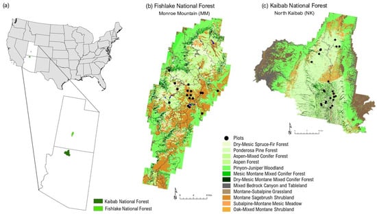
Figure 1.
(a) Location of study sites in the USA. Monroe Mountain (Fishlake National Forest) in Utah and North Kaibab National Forest in Arizona. Detailed maps show forest types derived from the USDA Forest Service’s Forest Inventory and Analysis Program for (b) MM and (c) NK. Note: Only sampled vegetation types are shown in the legend. Full classification available from LANDFIRE EVT 2024.
NK is lower in elevation than MM, with the former ranging from 899 to 2807 m (mean = 2159 m), and the latter ranging from 1707 to 3420 m (mean = 2673 m). It is also warmer than MM, with NK’s mean annual temperature of 9.9 °C versus MM’s 5.8 °C, according to PRISM 30-year (1991–2020) normals. Furthermore, NK is drier than MM, with NK typically receiving 491 mm of precipitation per year and MM receiving 545 mm.
According to LANDFIRE 2024 Existing Vegetation Type data, the most abundant vegetation type groups in MM include Montane Sagebrush Shrubland/Steppe (Artemisia tridentata), Pinyon–Juniper Woodland (Pinus edulis, Juniperus osteosperma), Aspen–Conifer (Populus tremuloides), and Aspen–Mixed Conifer Forests. In NK, dominant vegetation types include Pinyon–Juniper Woodland/Shrubland, Ponderosa Pine Forest (Pinus ponderosa), Sagebrush Shrubland, Dry-Mesic Montane Mixed Conifer Forest, Aspen–Mixed Conifer Forest, and Oak–Mixed Montane Shrubland (Quercus spp.). Table 1 provides a comparative overview of the vegetation type groups represented in the sampled plots at MM and NK.

Table 1.
Vegetation type groups sampled at MM and NK, based on LANDFIRE 2024 Existing Vegetation Type data. Table shows percentage area covered by each vegetation group within the corresponding study area (MM or NK), as well as number of plots sampled in each group.
By using two distinct study locations, we were able to assess the robustness and accuracy of the Random Forest (RF) model developed to predict fuel structure. This approach permitted evaluation of the model’s performance in different environments, thus providing valuable information on its generalizability and potential for broader application across landscapes.
2.2. Fuel Load Measurements
In July 2023, we established forty circular plots with a radius of 12.5 m (0.05 hectares), including 17 at MM and 23 at NK. Each plot was divided into four quadrants (NE, SE, SW, and NW) by two perpendicular transects, each 25 m long and oriented north/south and east/west. Additionally, a smaller subplot with a radius of 6.25 m (0.01 hectares) was defined (Figure 2a). All trees with diameter at breast height (DBH), taken at a height of 1.37 m, larger than 10 cm were tallied in the plot, and species, DBH, and health status (healthy, unhealthy, and dead) were recorded. For trees with a common base and multiple stems diverging below DBH, we calculated a single DBH by summing the individual cross-sectional areas of each stem and then converting this summed area into an equivalent diameter. This single DBH provides a value that represents the same cross-sectional area as the combined stems, ensuring that it accurately reflects the total biomass, though it may slightly underestimate canopy structural attributes due to the simplified representation of stem architecture. Height, crown width (averaged from two perpendicular crown measurements), and live and dead crown base height were recorded for a representative subset of trees, comprising at least 10% of the individuals of each species within each plot. Saplings (3 cm ≤ DBH < 10 cm) and seedlings (DBH < 3 cm), collectively referred to as “small trees”, were tallied following the same sampling protocol in the subplot. We imputed height, live and dead crown base heights, and crown width on the unmeasured trees using the missRanger() function from the R “missRanger” package (version 2.6.1) [35]. This method performs multivariate imputation using a combination of random forests and the MICE (Multivariate Imputation by Chained Equations) framework [36,37]. Specifically, missRanger applies chained random forest models to predict missing values based on the observed data, using predictive mean matching to preserve realistic distributions and avoid implausible values. This approach has shown high performance in handling complex, non-linear relationships and interactions between variables in ecological datasets. Summary statistics of forest structure across MM and NK plots are presented in Table A1.
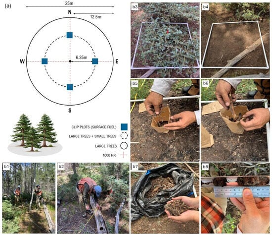
Figure 2.
Summary of field data collection methods: (a) diagram illustrating the sampling design and spatial arrangement of plots for large trees, small trees, and surface fuel clip plots; data were collected using different plot sizes and layouts for large trees (b1), 1000 h (b2), and surface fuels (b3–b8).
Diameter and decay class were recorded for the 1000 h fuels (i.e., coarser wood debris 7.6 cm in diameter) using the planar intercept technique, as outlined by [38] (Figure 2(b1,b2)). Four 1 m × 1 m clip plots were placed 6.25 m from the plot center in the north, south, east, and west directions (Figure 2a) and fine downed wood debris (i.e., dead branches ≤ 7.6 cm in diameter), herbaceous plants, shrubs, litter, and duff were measured. Within these clip plots and before any disturbance, litter and duff depths (in mm) were measured at the four corners using a ruler and soil probe respectively. Following that, herbaceous (grass and forbs) and shrubs were collected and categorized by health status as either “live” or “dead” (Figure 2(b3,b4)). Downed woody debris was collected and weighed separately in the field by categories defined as 1 h fuels (<6.35 mm), 10 h fuels (6.35–25.4 mm), and 100 h fuels (25.4–76.2 mm) (Figure 2(b5,b6)). Finally, litter and duff were collected and weighed separately (Figure 2(b7,b8)). Litter was defined as the forest floor layer consisting of fallen leaves, needles, cones, bark chunks, dead moss, lichens, herbaceous stems, and flower parts. Duff was considered the organic forest floor layer just beneath the litter, composed of partially and highly decomposed litter and other organic material [39]. For all fuel types, the total sample weight was measured in the field. A subsample was collected, weighed, and oven-dried in the lab, so that fuel moisture content was calculated. Dry biomass for each fuel category was then calculated using derived conversion factors.
To compute tree biomass (TB), species were categorized into taxonomic groups following the classification by [40] each with a specific allometric equation. However, these equations were developed exclusively for trees and saplings with a DBH greater than 3 cm. In the case of seedlings, it was necessary to apply an adjustment factor. The employed equations are outlined below (Equations (1) and (2)), and all the parameters used for calculations are provided in Table A2.
where TB is tree biomass (kg) for (1) trees with a DBH of 3 cm and larger or (2) trees with a DBH less than 3 cm; Exp = exponential function; Adj_Fac is an adjustment factor; and β0, β1 are regression coefficients or parameters specific to each species group.
TB (DBH ≥ 3 cm) = Exp (β0 + β1 × log (DBH))
TB (DBH < 3 cm) = Exp (β0 + β1 × log (DBH)) × Adj_Fac
To estimate the biomass of components (foliage, stem bark, stem wood, and branches) we applied the Component Ratio Method [41]. Species were categorized into two groups: hardwood and softwood and the ratio of each component was computed for each tree and sapling (Equation (3)). For seedlings, we utilized the average ratio derived from larger individuals. A comprehensive overview of these calculations is provided in Table A3.
where ratioi is the proportion of component i (such as foliage, stem bark, or stem wood) relative to the total biomass for saplings and trees, Exp is an exponential function, and γ0, γ1 are regression coefficients or parameters specific to each subgroup. Branch biomass was estimated by subtracting the biomass allocated to foliage, stem bark, and stem wood from the total aboveground biomass (AGB).
ratioi = Exp (γ0 + γ1/DBH)
We then multiplied the tree biomass by the computed ratio for each component. Branch biomass was calculated by subtracting the biomass of the stem bark, stem wood, and foliage from the total tree biomass. In addition to biomass, we identified a set of fuel structure and fuel load variables that could significantly impact fire behavior (Table A4).
2.3. LiDAR Data Acquisition
Although MLS and TLS data were collected from the same plots, they were not always acquired simultaneously. In most cases, MLS scanning was conducted immediately before or after TLS scanning on the same day. However, some scans occurred on different days due to logistical constraints. All data collection took place during the same field campaign and within the same season to minimize differences in vegetation structure and phenology. We acknowledge that small variations in weather conditions could have introduced subtle differences in the resulting point clouds. Nevertheless, the overall effect is expected to be minimal given the short time intervals and consistent seasonal conditions.
2.3.1. Mobile Laser Scanning (MLS)
MLS data were collected using two different sensors, a GeoSLAM ZEB Horizon (GeoSLAM Ltd., Nottingham, UK) and an Emesent Hovermap ST (Emesent, Milton, QLD, Australia). Although both sensors operate in similar frequency ranges (300,000 pts/s) and support dynamic scanning via SLAM, they differ in beam divergence, maximum range, and SLAM processing software, which may affect data quality under complex forest conditions [42] (Table 2).
Table 2.
Technical specifications for GeoSLAM ZEB Horizon and Leica BLK360.
We initiated the MLS scans at the center of each plot, consistently beginning our trajectory by walking north. This directionality is crucial for leveraging the walking trajectory in georeferencing to accurately identify targets. The MLS was operated in the backpack configuration throughout all scans. We walked through a theoretical flower petal design, doing a large loop, resembling a ‘major flower petal’, around the north target and then returning to the plot center. Subsequent scans involved walking slightly smaller loops (‘minor flower petals’) towards the northeastern edge of the plot and back, followed by similar patterns to the east and southeast, south, and southwest, and west and northwest directions. After completing all eight ‘petals’, a final circumferential walk around the entire plot edge was conducted, concluding the scan back at the plot center. This systematic approach not only ensures consistent data collection across plots but minimizes occlusion, improving representation of forest structure (Figure 3a). Data collection times varied substantially across plots. Scanning itself typically took 5–15 min; however, when including preparation time, the process could take up to 40 min depending on the vegetation density and plot conditions. Lower-fuel, sparsely vegetated, and less topographically diverse plots required significantly less time, while higher-fuel, densely vegetated, or steeper plots took considerably longer to complete.
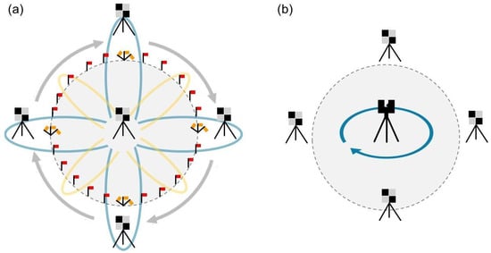
Figure 3.
LiDAR data collection methodology using (a) MLS and (b) TLS.
2.3.2. Terrestrial Laser Scanning (TLS)
We scanned the same plots using the Leica BLK360 (Leica Geosystems AG, Heerbrugg, Switzerland), an affordable terrestrial laser scanner capable of capturing high-resolution 3D point clouds [29]. Detailed specifications of the device are provided in Table 2. To conduct the scanning process, we placed the BLK as close as possible to the center of each plot (Figure 3b). In terms of data collection time, the BLK process was considerably faster than MLS, with preparation and scanning typically taking less than 10 min, of which only ~30 s were required for the scanning itself.
2.4. LiDAR Data Processing
To georeference both the MLS and TLS point clouds, reflective targets were positioned at the cardinal directions—north, south, east, west—and at plot center. These targets were designed with reflective material, allowing for easy identification in the point cloud using the intensity of the LiDAR return. GPS data was collected at each target location with high accuracy by using a Trimble Geo7x (Trimble Inc., Sunnyvale, CA, USA) or a Trimble R2 receiver (Trimble Inc., Sunnyvale, CA, USA). During processing, we used CloudCompare (version 2.13.2 Kharkiv) to align the target positions in the point cloud with their corresponding GPS coordinates. This process ensured precise georeferencing and accurate spatial alignment of the point cloud data. Next, we used the ‘lidR’ package in R (version 4.3.3) [43] to conduct the subsequent processing steps. Initially, we cropped the point clouds into a circular section with a 20 m radius to reduce data volume and decrease processing time. We then filtered out duplicate points and removed noise. For ground point classification, we performed multiple iterations of ‘lasground’, ‘lasclassify’ and ‘las2las’ from LAStools (version 230330) [44]. This iterative approach progressively reduced the point cloud, decreasing the percentage of negative heights, and improving ground classification and the quality of the digital terrain model (DTM). Based on our initial testing, this method yielded superior results compared to other algorithms and parameters applied in R, such as the Progressive Morphological Filter [45], Cloth Simulation Filter [46], and Multiscale Curvature Classification [47]. In R, we generated the DTM using a triangulated irregular network algorithm, normalized the data by subtracting the DTM, and finally cropped the data to the plot boundaries for metric generation. Figure 4 provides an overview of the point clouds from TLS and MLS, offering a visual comparison of the data collected from both sensors.
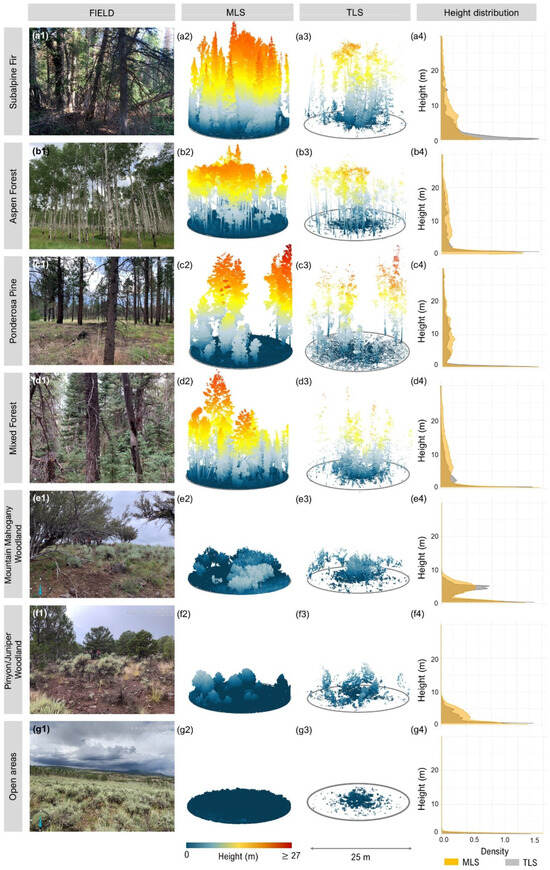
Figure 4.
Representative vegetation types across field sites (a1–g1); corresponding 3D point clouds from mobile laser scanning (MLS; a2–g2) and terrestrial laser scanning (TLS; a3–g3); and vertical height distributions of LiDAR returns (a4–g4). MLS point clouds show more continuous vertical profiles and fewer occlusion gaps, especially in dense forest types, due to dynamic scanning trajectories. In contrast, TLS point clouds are more affected by occlusion and exhibit sparser representation in upper canopy layers, particularly in complex stands like Subalpine Fir (a3) and Mixed Forest (d3). Height distribution plots (a4–g4) illustrate the relative density of returns per height bin (in meters), with MLS (orange) generally showing broader vertical coverage and more uniform return distribution across canopy layers than TLS (gray). This highlights the influence of scanning strategy on structural representation and explains the differences in fuel attribute estimation performance between sensors.
We extracted two sets of LiDAR metrics at the plot level: height metrics and density metrics. The height metrics include height percentiles, maximum, and mean heights, variance, standard deviation, coefficient of variation, skewness, and kurtosis of height. The density metrics included the percentage of non-ground returns in different strata, canopy cover, and canopy relief ratio. Canopy density was derived directly from the normalized point cloud using the cloud_metrics() function in the lidR package. We calculated density as the proportion of LiDAR returns above a series of fixed height thresholds relative to the total number of returns within each plot. These thresholds approximate structural strata but do not isolate discrete vertical layers; instead, they represent cumulative canopy presence above each height. This approach follows the method described by Hudak et al. (2020) [48] and allows consistent structural comparisons across platforms.
Canopy cover metrics were derived from the Canopy Height Model (CHM) raster generated at 0.5 m spatial resolution. For each threshold, we calculated the proportion of CHM pixels with values equal to or greater than that height, relative to the total number of valid pixels within the plot. These included fractional cover at multiple thresholds, consistent with previous studies on vertical canopy structure. The canopy relief ratio (CRR) was calculated as the difference between the mean and minimum CHM values, divided by the difference between the maximum and minimum values. This metric quantifies vertical complexity, ranging from values near 0 in uniform canopies to values approaching 1 in structurally diverse plots. All LiDAR metrics and corresponding thresholds are listed in Table A5.
2.5. Fuel Load Modeling
2.5.1. Selection of LiDAR Metrics
The variable selection process was conducted in two stages. First, we applied Pearson’s correlation coefficient to identify and remove highly correlated LiDAR variables. To do this, we used the base R function “cor”, to compute the correlation matrix, which was visualized through a correlogram generated with the corrplot package [49]. The “caret” R package [50] was then used to identify and exclude highly correlated variables via the “findCorrelation” function. This allowed us to refine the models by retaining only predictors that contributed unique, non-redundant information. A correlation threshold of 0.9 was defined, meaning that any two variables with a correlation coefficient greater than or equal to 0.9 were considered highly correlated, and one of them was removed from the modeling development. This threshold was chosen based on standard practices in multivariate modeling to minimize multicollinearity, which can inflate errors and distort model interpretations.
In the second stage, we applied the “rf.modelSel” routine from the “rfUtilities” R package [51]. This method calculates normalized predictor variable importance scores, such as the Model Improvement Ratio (MIR), which range from 0 (least important) to 1 (most important). This approach was used to identify the most relevant LiDAR metrics for each fuel variable, ensuring that the final predictors contribute significantly to the predictive power while minimizing redundancy among variables.
2.5.2. Model Development and Assessment
We fitted Random Forest (RF) models using the ‘randomForest’ package in R [51,52,53,54], primarily using the default parameters. Each model was built with 500 trees (ntree = 500) and the default number of variables randomly selected at each split (mtry) was used unless otherwise noted. For each fuel metric (response variable), an individual univariate RF model was trained using a subset of predictor variables selected through an iterative variable selection procedure. This procedure used repeated bootstrapping (30–50 iterations) to identify the most consistently important predictors across iterations, based on scaled permutation importance. Model performance was evaluated using out-of-bag (OOB) predictions as well as through additional bootstrapped cross-validation with 70/30 train/test splits across 500 iterations. No multivariate models were used; each fuel metric was modeled independently.
To assess the performance of the RF models, we used several evaluation metrics. The coefficient of determination (R2) was calculated to quantify the proportion of variance in the observed data explained by the model, providing an indicator of goodness-of-fit. Additionally, we used the root mean square error (RMSE) to measure the typical magnitude of prediction error, which quantifies the average discrepancy (in absolute terms) between observed and predicted values. RMSE was expressed in relative terms (%RMSE), as a percentage of the mean observed value, to standardize comparisons across different response variables. We also calculated bias to capture the average directional difference between observed and predicted values, indicating any consistent under- or overestimation by the model. Together, these metrics (Equations (4)–(8)) provide a comprehensive evaluation of model accuracy, precision, and reliability.
where Ŷi is the estimated value; Yi is the observed value; n is the number of samples; and Ȳ is the mean of the observed values.
R2 = 1 − (Σ (Yi − Ŷi)2)/(Σ (Yi − Ȳ)2)
RMSE (Abs) = √(Σ (Ŷi − Yi)2/n)
RMSE (%) = (RMSE/Ȳ) × 100
Bias (Abs) = (1/n) Σ (Ŷi − Yi)
Bias (%) = (Bias/Ȳ) × 100
To statistically compare the predictive performance of TLS and MLS models, we conducted a paired t-test using the coefficient of determination (R2) for each fuel attribute. Prior to the test, we verified the assumption of normality for the paired differences using the Shapiro–Wilk test. As the normality assumption was met (p = 0.71), a parametric paired t-test was applied. Along with p-values, 95% confidence intervals were reported to quantify the uncertainty of mean differences. The magnitude of performance difference was interpreted using the average effect size (mean R2 difference), which provides a practical assessment of the improvement from TLS to MLS.
2.5.3. Transferability of the Fuel Load Models
We conducted a transferability test to evaluate the generalizability and robustness of our models across different geographic locations. Specifically, we trained our RF models using data from one site (e.g., NK) and subsequently validated them using data from the other site (e.g., MM). To ensure consistency in evaluation, we used the same performance metrics—R2, relative RMSE (%), and relative bias (%)—as were used in the original model assessments.
All steps of the methodology are summarized and illustrated in Figure 5, providing a visual overview from data collection in the field to data processing and modeling.
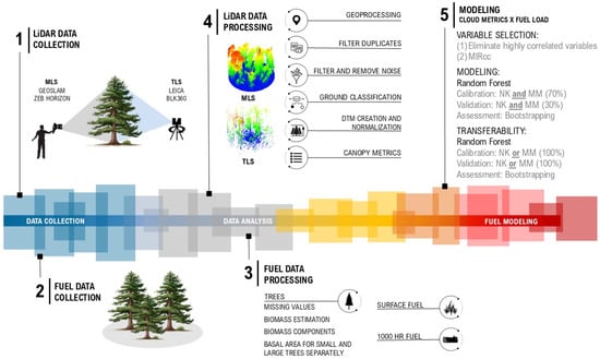
Figure 5.
Study design overview: data collection, data analysis, and fuel modeling.
3. Results
3.1. Selection of LiDAR Metrics
The first stage of the variable selection process, which was based on Pearson correlation, reduced the number of candidate metrics from 56 to 14 for MLS and to 18 for TLS (Figure 6). Out of the selected metrics, ten density metrics (COV_f1m, COV_f5m, COV_f10m, DNS_10m, CRR, DMEAN, STRATUM0, STRATUM1, STRATUM2, STRATUM3) and three height metrics (H05TH, HNMODES, HKUR) were common to both MLS and TLS models.
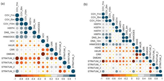
Figure 6.
Pearson correlation matrix (r) among variables derived from MLS (a) and TLS (b). Only variables with pairwise correlations below the high collinearity threshold (|r| < 0.9) are shown in each panel.
The second stage of the variable selection process involved applying the MIR method (Figure 7). Across both sensors, there is a notable predominance of metrics related to vegetation cover and density, such as cover fractions at 5 m and 10 m and canopy density at 10 m. These metrics frequently appear across the models for various fuel components, suggesting that they are crucial for understanding the spatial structure of fuel loads, regardless of the sensor being used.
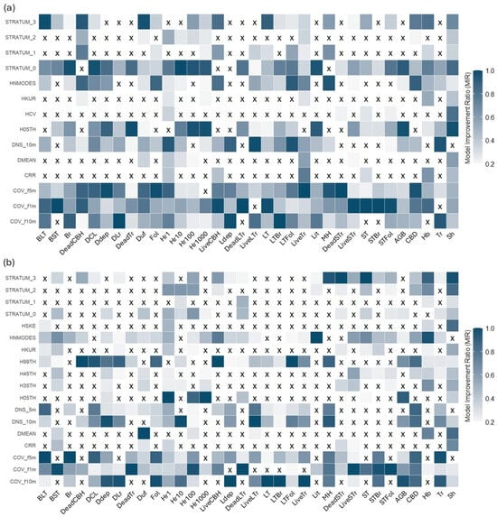
Figure 7.
Mean Model Improvement Ratio (MIR) of metrics preselected based on Pearson’s correlation. Metrics with an MIR of 0.2 or higher were selected for inclusion in the modeling process. (a) refers to MLS, and (b) refers to TLS. Cells with ‘X’ show metrics that were excluded by the method.
3.2. Model Assessment
Paired t-tests comparing model performance across fuel attributes showed that MLS models significantly outperformed TLS models in terms of R2 (mean difference = 0.08, 95% CI: 0.047–0.113, p < 0.001). These results confirm the consistent advantage of MLS over single-scan TLS configuration (Figure 8, Table A6). In this group, MLS achieved a higher average R2 (0.55) compared to TLS (0.45), and a lower average %RMSE (76.66% vs. 90.76%), indicating more accurate predictions. Bias values were also lower for MLS (mean = 5.42%) than for TLS (mean = 4.19%), though variability remained.
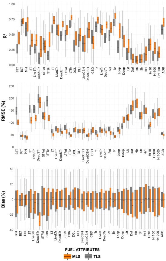
Figure 8.
Validation performance assessment (R2, %RMSE, and %Bias) in 500 iterations of models used to estimate fuel metrics. Whiskers extend to 1.5 × interquartile range. Outliers were excluded for clarity.
For surface fuel components, including downed wood (1 h, 10 h, 100 h, 1000 h), litter, and litter depth, the MLS models again showed improved performance, with higher average R2 (0.30 vs. 0.25 for TLS) and slightly higher %RMSE (129.18% vs. 122.63%). Notably, bias levels remained similar between the two platforms (MLS = 16.27%, TLS = 16.56%), suggesting both models struggled similarly with these more variable and spatially heterogeneous fuels.
In contrast, ground fuels such as herbaceous biomass (Hb) and shrub biomass (Sh) were poorly predicted by both platforms, with low R2 values (0.11 for TLS, 0.12 for MLS) and high %RMSE (160.95% for TLS, 164.67% for MLS). These results highlight the challenges of modeling fine-scale surface components using airborne or terrestrial laser scanning.
When considering total aboveground biomass (AGB), the MLS model again demonstrated better predictive power (R2 = 0.69; %RMSE = 49.11%) compared to TLS (R2 = 0.57; %RMSE = 54.64%), with MLS also producing lower bias.
3.3. Transferability Model Performance
Table A7 and Table A8 summarize the predictive performance of MLS and TLS models when transferred between sites from NK to MM and vice versa (Figure 9 and Figure 10). Table A9 presents the percent change in R2 after model transfer, with positive values indicating improved performance and negative values reflecting a decline.
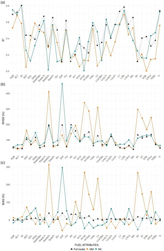
Figure 9.
Differences in (a) R2, (b) RMSE (%), and (c) bias (%) values between transferred and full models for the MLS system. “MM” represents models trained at Monroe Mountain and tested at North Kaibab, while “NK” represents models trained at North Kaibab and tested at Monroe Mountain.
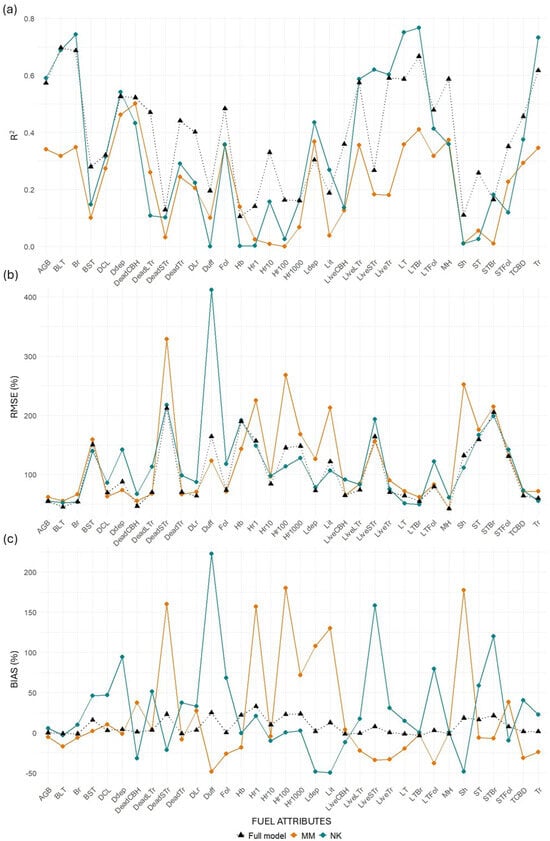
Figure 10.
Differences in (a) R2, (b) RMSE (%), and (c) bias (%) values between transferred and full models for the TLS system. “MM” represents models trained at Monroe Mountain and tested at North Kaibab, while “NK” represents models trained at North Kaibab and tested at Monroe Mountain.
MLS models for canopy-related variables retained relatively good performance when transferred from NK to MM, with minor losses in R2 for key metrics such as BLT (−3.49%), Br (−0.53%), and Tr (−1.75%). Some variables even improved, including LiveLTr (+12.01%), CBD (+24.98%), and STFol (+40.20%). However, when transferred from MM to NK, losses were more substantial across the board (e.g., Br: −27.36%; LiveLTr: −37.55%; STBr: −99.43%). This asymmetry suggests that models trained in the more structurally diverse NK site may generalize better than those trained in MM. TLS models performed worse than MLS in both directions and showed extreme declines in some metrics when transferred from MM to NK (e.g., BLT: −54.35%, STBr: −93.6%).
Surface fuel models were the most inconsistent. MLS models showed surprising gains when transferred from NK to MM (mean R2 change = +75.25%), largely due to strong positive responses in Sh (+111.32%) and Hb (+39.17%). However, in the reverse direction (MM to NK), the average R2 gain was more modest (+17.03%), and TLS models performed poorly in both directions, particularly from NK to MM (−94.40%).
Ground fuels exhibited high variability. MLS models again showed better transferability from NK to MM (mean = +7.89%), with gains in metrics such as Lit (+52.21%), Hr10 (+23.62%), and Hr1 (+20.34%). The transfer from MM to NK was much less successful, with an average decline of 28.83%, including large losses in Hr10 (−83.68%) and Lit (−79.44%). TLS models suffered significant performance losses in both directions, especially from MM to NK (−57.07%).
Total AGB also reflected the general trend. MLS models showed a performance gain of 8.13% when transferred from NK to MM and a decline of 23.68% from MM to NK. TLS models had lower overall transferability, with a small gain (+2.93%) in the NK to MM direction, but a marked loss (−40.61%) when transferred from MM to NK.
4. Discussion
4.1. Model Performance Analysis
Consistent with the findings of Bienert et al. (2018), our results confirm the superior performance of MLS models, which consistently outperformed TLS across most fuel attributes, especially for canopy fuels and standing woody biomass [32]. These attributes are especially relevant for understanding the vertical distribution of vegetation layers, which strongly influences fire behavior. Denser or taller canopies increase fuel availability and the potential for fire propagation.
One key difference between the sensors lies in their data acquisition strategies. The MLS sensor, moving through the plot, has the potential to collect data from a broader range of viewing angles, which can improve structural characterization, especially near the ground. However, its ability to detect fine surface fuels, such as grass and litter, is still limited by factors like sensor ranging accuracy, vegetation occlusion, and SLAM drift. In our models, MLS more frequently selected lower-stratum metrics such as Stratum_0, suggesting better relative sensitivity to near-ground structure compared to TLS. However, both MLS and TLS performed poorly in predicting surface and ground fuel attributes, including fine fuels (1 h, 10 h, litter depth), and coarser downed woody classes (100 h and 1000 h). This highlights the persistent challenge of using LiDAR to estimate understory and ground-level fuel components.
The challenges with TLS performance are likely due to occlusion effects. In this study, only one scan per plot was acquired from a fixed position at plot center, limiting visibility, especially of understory and ground-level fuels farther from the scanner. Although TLS remains appealing due to its operational simplicity and affordability, its limitations are clear in this configuration. A multi-scan approach could mitigate occlusion and improve model quality, but this would require more expertise and time, potentially surpassing the complexity of MLS systems, which benefit from automated SLAM-based registration. Future work should explore flexible TLS scanning protocols. Designing scan arrangements adapted to varying forest types could help balance data quality, field efficiency, and ease of processing, especially in dense or multi-layered forests.
4.2. Transferability of Model Performance
Model transferability varied across fuel types, LiDAR platforms, and transfer directions. Canopy-related attributes, such as total tree biomass (Tr) and aboveground biomass (AGB), showed the highest transferability, particularly in MLS models. For instance, an AGB model trained in NK and applied to MM even improved slightly (+8.13% in R2), while the reverse direction experienced a moderate decline (−23.68%). In contrast, surface and ground fuel metrics—especially 1, 10, 100, and 1000 h fuels, duff, and litter—transferred poorly, often showing R2 drops greater than 80%, particularly when using TLS. These patterns reflect the inherent difficulty of predicting fine fuels even within a single site, likely due to both their ecological variability and the limitations of sensor sensitivity to ground-level signals.
Several factors help explain the observed asymmetry in transfer performance between NK and MM. NK plots featured a larger sample size, more structural heterogeneity, and greater canopy complexity, which likely provided more robust training data and improved generalization capacity. In contrast, MM plots were more structurally homogeneous, and four plots lacked any trees, limiting the diversity and applicability of training data. Additionally, differences in species composition, understory density, and terrain between sites may have influenced the sensitivity of LiDAR metrics, especially for strata close to the ground, where occlusion and clutter are more problematic.
Methodological choices also shaped transferability outcomes. TLS data were collected from a single fixed-position scan per plot, which restricted the sensor’s ability to detect understory and ground fuels due to occlusion, especially in denser stands. While this protocol was efficient and cost-effective, it reduced spatial coverage and may explain the poorer performance and generalization of TLS-based models. In contrast, MLS scanning benefited from dynamic movement and automated SLAM registration, enabling broader plot coverage and more complete representation of vegetation structure. This advantage was reflected in the overall higher robustness of MLS models across transfer scenarios. Future studies may improve TLS model performance by adopting multi-scan or rotating station protocols that increase spatial resolution without compromising field efficiency.
Interestingly, some transferred models outperformed their full-model counterparts. In certain cases, models trained at one site and applied to another yielded higher predictive accuracy than those trained on pooled data from both sites. This suggests that combining data from ecologically distinct areas may introduce noise or lead to overfitting of site-specific patterns, reducing generalizability. Targeted models, therefore, may offer better performance for particular forest structures or fuel components, despite lacking broader applicability.
While the statistical comparisons between TLS and MLS models revealed significant differences in performance (p < 0.001), the mean R2 difference was approximately 0.08 in favor of MLS—an effect size with practical relevance, particularly for fuel mapping in operational contexts. This performance gap was more pronounced for canopy-related metrics than for surface fuels, indicating that MLS is better suited to capturing vertical structure relevant to aboveground biomass and tree-based attributes.
One important limitation of our modeling framework is the exclusion of environmental covariates. To isolate the performance of LiDAR-derived structural metrics, we deliberately omitted predictors such as elevation, slope, aspect, or species identity. While this simplification allowed for a direct comparison between platforms, it likely contributed to the poor transferability of fine fuel and surface attributes, which are often strongly influenced by microtopography and ecological gradients. Future work should consider incorporating such covariates to improve predictive accuracy and interpretability.
From an applied perspective, model scalability remains a central challenge. Although our analysis focused on plot-level estimates, landscape-scale fuel mapping requires spatially explicit data. A promising direction for upscaling involves calibrating ground-based LiDAR models with spaceborne LiDAR and multispectral imagery to generate continuous maps of fuel structure. Such integration would enhance the operational utility of LiDAR-based fuel models for fire risk assessment, fuel treatment planning, and ecosystem monitoring across diverse forest types.
4.3. Ecological Considerations and Fire Management Implications
We demonstrated that MLS models were highly effective in predicting key structural and canopy fuel attributes critical for modeling crown fire initiation and propagation. These include canopy base height (live and dead), canopy bulk density, dead crown length, mean canopy height, and crown foliage and branch biomass, all of which are essential for determining vertical fuel continuity, ignition potential, and canopy fire spread dynamics. Such attributes are fundamental for fire behavior models and play a central role in fire management strategies aimed at reducing the risk of high-severity wildfires. Species like spruce and fir, which have highly flammable low branches, introduce a significant dynamic in fire ecology [55]. These species are notably vulnerable to fire events, often being seriously affected. Their survival depends heavily on post-fire regeneration, and without successful regeneration, any competitive advantage these species might have gained through fire adaptation is lost. The ability of a forest to regenerate after fire events is vital, as species that successfully regenerate can significantly alter forest composition and fuel availability for future fires [56]. In this context, the improved performance that MLS offers over the TLS single scan in representing these structural elements provides a clearer understanding of the conditions that influence fire risk.
Conversely, the prediction of surface fuels, which play a key role in fire spread, was challenging for both MLS and TLS. A key limitation is the underrepresentation of fine surface fuels such as litter and duff, which are inherently difficult to detect due to their fine structure and low vertical separation from the ground. While understory occlusion can affect the detection of larger surface elements, the inability to resolve fine fuels is primarily due to LiDAR’s limited capacity to penetrate and distinguish such elements. Even MLS, which reduces occlusion by capturing data dynamically [57], suffers from increased SLAM-related noise and lower ranging accuracy, further limiting its ability to quantify fine surface fuels. As a result, accurate surface fuel characterization in dense forests may still require complementary ground-based or alternative remote sensing methods.
The flammability of dead material also presents a dynamic that evolves over time. Initially, trees with intact dead branches and needles are highly flammable due to their low moisture content. These fine fuels ignite easily, contributing significantly to fire spread to and throughout the canopy. However, as the needles and smaller branches drop, the flammability of standing trees decreases. Although the larger branches and boles remain consumable during fire events, they play a reduced role in propagating fire. This shift is essential for fire management, highlighting the need to assess standing trees not only for their immediate fire risk but also for their long-term contribution to fuel loads. The dead/live ratio, which was accurately predicted by MLS models in our study, is a key indicator of this balance. Fire managers may need to prioritize the removal or treatment of trees with intact fine fuels, as they are more likely to contribute to rapid fire spread compared to trees with dropped fine fuels.
From a fire management perspective, our findings provide actionable insights for selecting LiDAR platforms based on specific operational goals. MLS is recommended for canopy-focused assessments—such as estimating total biomass, canopy base height, and canopy bulk density—especially when working across heterogeneous or large-scale landscapes where model generalization is critical. TLS, while more limited in spatial coverage due to occlusion and fixed-position constraints, may be more cost-effective and suitable for site-specific inventories, particularly when used with enhanced scanning protocols (e.g., multi-position scans).
Operational decisions should weigh cost, accuracy, and logistics. MLS systems offer faster data collection and broader coverage but require higher investment and technical expertise. TLS is less expensive and simpler to deploy but may demand more time in the field and produce lower model transferability. A hybrid strategy may be most effective: using MLS for regional fuel mapping and TLS for targeted verification or detailed analysis in priority zones.
Finally, the limited transferability of fine fuel predictions suggests that LiDAR alone may be insufficient for accurate surface fuel assessment in all contexts. Fire managers should consider integrating ecological covariates or complementary field sampling methods when surface fuel characterization is critical to decision-making.
4.4. Limitations and Future Directions
Despite the valuable insights gained from this comparative analysis, several limitations must be acknowledged. First, seasonal variation in vegetation structure, such as changes in leaf phenology, moisture content, or herbaceous layer density, may have affected LiDAR returns, particularly in surface and understory layers. Our data were collected within a limited seasonal window, but phenological stage can influence occlusion, reflectance, and biomass estimates, especially in deciduous or mixed systems.
Second, understory vegetation likely contributed to occlusion effects, especially for TLS, which relies on a single fixed scan position. Dense shrubs and grasses can obscure lower fuel layers and affect the accuracy of structural metrics derived. While MLS partially overcomes this with dynamic scanning paths, both systems remain limited in capturing fully occluded or low-contrast vegetation elements.
Third, both MLS and TLS struggled to accurately characterize fine surface fuels (e.g., litter, duff, herbaceous biomass), which are challenging to detect due to their small size, proximity to the ground, and low point cloud contrast. This limitation restricts the use of ground-based LiDAR alone for complete fuel profiling, suggesting a need for complementary data sources or enhanced scanning protocols.
Future work should explore seasonal data acquisition, flexible TLS configurations, and integration with multispectral or hyperspectral data to improve fuel detection across strata and fuel types.
5. Conclusions
In conclusion, this study highlights the effectiveness of both TLS and MLS in estimating plot-level fuel loads across different vegetation strata, offering valuable guidance for selecting LiDAR metrics in predictive modeling. Our findings show that MLS consistently outperformed TLS, particularly for canopy-related attributes, due to its ability to capture structural information from multiple angles as it moves through the plot.
However, the TLS system used here relied on a single-scan setup, which, while operationally efficient and cost-effective, introduced significant occlusion, especially in complex or dense vegetation. This limited its ability to accurately detect fuels in lower strata and contributed to its overall lower performance. Still, TLS demonstrated potential as a practical tool, particularly for users with limited budgets or those seeking simpler field protocols.
With the adoption of multi-scan TLS strategies, which help reduce occlusion and improve structural detail, the predictive capacity of TLS could be substantially enhanced, though this comes at the cost of greater field effort and processing complexity. For forest managers and practitioners, TLS remains a viable option, especially when workflows are adapted to balance efficiency and data quality.
Ultimately, by recognizing the trade-offs between mobility, coverage, and resolution across LiDAR platforms, future studies can build on these findings to refine data collection strategies, improve model performance, and strengthen the role of LiDAR in fire ecology and forest management.
Author Contributions
E.K.L.B., C.A.S., A.T.H. and M.J.C. contributed to the conceptualization of the study. E.K.L.B., C.A.S., A.T.H., K.M.B., M.J.C., N.S.-L., M.B.S., B.C.B., I.T.B., G.M.d.S., J.X., J.F.E. and K.D.R. participated in field data collection. E.K.L.B., K.M.B. and K.D.R. contributed to laboratory data processing and data organization. E.K.L.B., C.A.S., M.J.C., J.F.E., F.M., C.H., A.P.D.C. and B.C.B. were involved in data analysis and modeling. E.K.L.B., C.A.S., M.J.C., B.C.B., F.M., E.N.B., N.S.-L., A.S., C.H., A.P.D.C., I.L.P., R.A.P., I.T.B., J.W.A. and J.V. contributed to the writing, interpretation, quality control, and revisions of the manuscript. C.A.S., A.T.H., J.W.A., E.N.B., F.M., A.S., R.A.P., B.C.B., J.V., E.R. and C.K. were responsible for funding acquisition. All authors have read and agreed to the published version of the manuscript.
Funding
This research was funded by the Joint Fire Science Program, “#22-2-02-15 EMS4D: Multi-Scale Fuel Mapping and Decision Support System for the Next Generation of Fire Management,” Francisco Mauro was supported by the Maria Zambrano’s Excellence Program (#E-42-2022-0000233) from the Ministry of Science and Innovation and funded by the University of Valladolid and European Union-Next Generation EU. The findings and conclusions in this publication are those of the authors and should not be construed to represent any official USDA or U.S. Government determination or policy.
Data Availability Statement
The data presented in this study are available on request from the corresponding author, as they are part of an ongoing research project. To protect the integrity of the ongoing work and prevent premature interpretation, the data cannot be made publicly available at this time. Access may be granted upon reasonable request, subject to approval by the project coordinators and in accordance with confidentiality agreements established with the participating institutions.
Conflicts of Interest
The authors declare that they have no known competing financial interests or personal relationships that could have appeared to influence the work reported in this paper.
Appendix A
Table A1.
Summary statistics of forest structure within established plots in MM (n = 17) and NK (n = 23), including tree count per plot, mean and maximum DBH (cm), mean and maximum tree height (m), percent cover in shrub, understory and canopy layers (%), dominant species (ABLA = Abies lasiocarpa, POTR = Populus tremuloides, CELE = Cercocarpus ledifolius, PIED = Pinus edulis, PIPO = Pinus Ponderosa, PIEN = Picea engelmannii), number of species (richness), and Shannon index (H′).
| Area | Plot | Tree Count | Mean DBH | Max DBH | Mean Height | Max Height | Shrub | Understory | Canopy | Dominant Species | Richness | H′ |
|---|---|---|---|---|---|---|---|---|---|---|---|---|
| MM | 1 | 94.0 | 18.0 | 42.4 | 9.6 | 21.1 | 17.0 | 71.3 | 11.7 | ABLA | 3 | 0.72 |
| 2 | 55.0 | 18.9 | 36.7 | 10.0 | 16.6 | 1.8 | 90.9 | 7.3 | POTR | 1 | 0.00 | |
| 3 | 0.0 | 0.0 | 0.0 | 0.0 | 0.0 | 0.0 | 0.0 | 0.0 | - | 1 | 0.00 | |
| 4 | 55.0 | 12.8 | 33.2 | 7.9 | 19.1 | 16.4 | 78.2 | 5.5 | POTR | 4 | 1.25 | |
| 5 | 16.0 | 28.0 | 46.1 | 13.4 | 22.0 | 12.5 | 50.0 | 37.5 | CELE | 1 | 0.00 | |
| 6 | 18.0 | 15.5 | 22.8 | 8.4 | 11.0 | 0.0 | 94.4 | 0.0 | POTR | 2 | 0.21 | |
| 7 | 64.0 | 11.4 | 33.5 | 6.7 | 16.4 | 32.8 | 64.1 | 3.1 | ABLA | 3 | 0.85 | |
| 8 | 43.0 | 18.3 | 41.7 | 9.6 | 18.7 | 4.7 | 88.4 | 7.0 | POTR | 1 | 0.00 | |
| 9 | 109.0 | 10.4 | 39.2 | 6.3 | 18.9 | 57.8 | 37.6 | 4.6 | ABLA | 2 | 0.42 | |
| 10 | 0.0 | 0.0 | 0.0 | 0.0 | 0.0 | 0.0 | 0.0 | 0.0 | - | 1 | 0.00 | |
| 11 | 0.0 | 0.0 | 0.0 | 0.0 | 0.0 | 0.0 | 0.0 | 0.0 | - | 1 | 0.00 | |
| 12 | 71.0 | 15.0 | 49.9 | 8.4 | 22.9 | 31.0 | 54.9 | 14.1 | ABLA | 5 | 1.25 | |
| 13 | 0.0 | 0.0 | 0.0 | 0.0 | 0.0 | 0.0 | 0.0 | 0.0 | - | 1 | 0.00 | |
| 14 | 18.0 | 23.6 | 58.5 | 12.3 | 24.4 | 11.1 | 66.7 | 22.2 | POTR | 2 | 0.21 | |
| 15 | 0.0 | 0.0 | 0.0 | 0.0 | 0.0 | 0.0 | 0.0 | 0.0 | - | 1 | 0.00 | |
| 16 | 8.0 | 33.8 | 61.2 | 12.7 | 28.6 | 25.0 | 12.5 | 50.0 | PIED | 3 | 0.74 | |
| 17 | 18.0 | 15.0 | 26.2 | 4.4 | 11.5 | 77.8 | 22.2 | 0.0 | PIED | 2 | 0.45 | |
| NK | 1 | 6.0 | 27.1 | 58.7 | 11.0 | 22.3 | 33.3 | 33.3 | 33.3 | PIPO | 1 | 0.00 |
| 2 | 9.0 | 42.0 | 63.8 | 21.0 | 29.8 | 11.1 | 11.1 | 77.8 | PIPO | 4 | 1.21 | |
| 3 | 57.0 | 10.2 | 47.0 | 5.6 | 22.4 | 56.1 | 40.4 | 3.5 | POTR | 4 | 1.21 | |
| 4 | 17.0 | 22.0 | 36.8 | 10.9 | 17.3 | 17.6 | 52.9 | 29.4 | PIPO | 1 | 0.00 | |
| 5 | 37.0 | 13.8 | 62.1 | 7.9 | 29.0 | 18.9 | 73.0 | 8.1 | PIPO | 1 | 0.00 | |
| 6 | 41.0 | 18.0 | 47.5 | 9.7 | 20.8 | 14.6 | 68.3 | 17.1 | POTR | 4 | 1.12 | |
| 7 | 16.0 | 20.6 | 49.3 | 10.8 | 22.2 | 6.3 | 68.8 | 18.8 | PIPO | 2 | 0.23 | |
| 8 | 51.0 | 13.3 | 41.7 | 7.2 | 14.3 | 23.5 | 76.5 | 0.0 | PIPO | 1 | 0.00 | |
| 9 | 40.0 | 13.3 | 47.5 | 7.4 | 22.6 | 62.5 | 17.5 | 20.0 | PIPO | 1 | 0.00 | |
| 10 | 240.0 | 9.8 | 22.6 | 6.3 | 14.8 | 35.0 | 65.0 | 0.0 | POTR | 4 | 0.27 | |
| 11 | 30.0 | 20.7 | 46.4 | 9.7 | 17.1 | 10.0 | 80.0 | 10.0 | PIED | 2 | 0.45 | |
| 12 | 50.0 | 17.9 | 46.5 | 9.2 | 19.2 | 6.0 | 90.0 | 4.0 | PIED | 3 | 0.27 | |
| 13 | 29.0 | 16.4 | 49.7 | 9.1 | 23.4 | 44.8 | 24.1 | 31.0 | PIED | 5 | 1.37 | |
| 14 | 35.0 | 22.4 | 116.5 | 10.7 | 30.2 | 28.6 | 48.6 | 22.9 | PIEN | 4 | 0.75 | |
| 15 | 33.0 | 19.3 | 47.8 | 10.4 | 24.4 | 36.4 | 39.4 | 24.2 | POTR | 3 | 0.93 | |
| 16 | 53.0 | 16.8 | 41.1 | 9.3 | 23.5 | 37.7 | 39.6 | 22.6 | POTR | 4 | 1.24 | |
| 17 | 30.0 | 26.0 | 113.9 | 13.0 | 34.1 | 13.3 | 56.7 | 30.0 | ABLA | 6 | 1.63 | |
| 18 | 33.0 | 14.0 | 51.6 | 8.5 | 29.0 | 36.4 | 51.5 | 12.1 | POTR | 4 | 0.84 | |
| 19 | 37.0 | 26.4 | 58.8 | 13.5 | 26.6 | 2.7 | 62.2 | 35.1 | PIPO | 5 | 1.36 | |
| 20 | 111.0 | 5.1 | 58.6 | 3.9 | 27.5 | 93.7 | 2.7 | 3.6 | POTR | 2 | 0.24 | |
| 21 | 0.0 | 0.0 | 0.0 | 0.0 | 0.0 | 0.0 | 0.0 | 0.0 | - | 1 | 0.00 | |
| 22 | 0.0 | 0.0 | 0.0 | 0.0 | 0.0 | 0.0 | 0.0 | 0.0 | - | 1 | 0.00 | |
| 23 | 0.0 | 0.0 | 0.0 | 0.0 | 0.0 | 0.0 | 0.0 | 0.0 | - | 1 | 0.00 |
Table A2.
Aboveground biomass (AGB) calculation parameters.
Table A2.
Aboveground biomass (AGB) calculation parameters.
| Species | Species Subgroup | Species Group | β0 | β1 | Adj. Factor |
|---|---|---|---|---|---|
| (sp_Sub) | (sp_Group) | ||||
| Abies concolor | Softwood | Abies ≥ 0.35 spg | −3.1774 | 2.6426 | 0.602 |
| Abies lasiocarpa | Softwood | Abies < 0.35 spg | −2.3123 | 2.3482 | 0.84 |
| Cercocarpus ledifolius | Hardwood | Rosaceae | −2.9255 | 2.4109 | NA |
| Juniperus osteosperma | Softwood | Cupressaceae | −2.7096 | 2.1942 | 0.352 |
| Picea engelmannii | Softwood | Picea < 0.35 spg | −3.03 | 2.5567 | 0.442 |
| Picea pungens | Softwood | Picea ≥ 0.35 spg | −2.1364 | 2.3233 | 0.442 |
| Pinus edulis | Softwood | Pinaceae | −3.2007 | 2.5339 | 0.352 |
| Pinus ponderosa | Softwood | Pinus < 0.45 spg | −2.6177 | 2.4638 | 0.434 |
| Populus tremuloides | Hardwood | Salicaceae ≥ 0.35 spg | −2.4441 | 2.4561 | 0.691 |
| Pseudotsuga menziesii | Softwood | Pseudotsuga | −2.4623 | 2.4852 | 0.526 |
| Robinia neomexicana | Hardwood | Fabaceae/Juglandaceae, other | −2.5095 | 2.5437 | 0.932 |
Table A3.
Calculation parameters for estimating component ratios of total aboveground biomass for hardwood and softwood species.
Table A3.
Calculation parameters for estimating component ratios of total aboveground biomass for hardwood and softwood species.
| Species Subgroup (sp_sub) | Biomass Component | β0 | β1 |
|---|---|---|---|
| Hardwood | Foliage | −4.0813 | 5.8816 |
| Stem bark | −2.0129 | −1.6805 | |
| Stem wood | −0.3065 | −5.424 | |
| Softwood | Foliage | −2.9584 | 4.4766 |
| Stem bark | −2.098 | −1.1432 | |
| Stem wood | −0.3737 | −1.8055 |
Table A4.
Fuel load and vegetation metrics at plot-level.
Table A4.
Fuel load and vegetation metrics at plot-level.
| Fuel Category | Metrics | Acronym | Description |
|---|---|---|---|
| Canopy fuels | Basal area (large trees) | BLT | m2/ha |
| Basal area (small trees) | BST | m2/ha | |
| Mean canopy height | MH | Average per plot (m) | |
| Dead crown length | DCL | Average per plot (m) | |
| Dead/Live ratio | DLr | ∑ (Dvol/(Lvol + Dvol)) | |
| Live canopy base height | LiveCBH | Average per plot | |
| Dead canopy base height | DeadCBH | Average per plot | |
| Canopy bulk density | CBD | Average per plot | |
| Trees | Tr | Sum per plot (Mg/ha) | |
| Live trees | LiveTr | Sum per plot (Mg/ha) | |
| Dead trees | DeadTr | Sum per plot (Mg/ha) | |
| Tree branches | Br | Sum per plot (Mg/ha) | |
| Tree foliage | Fol | Sum per plot (Mg/ha) | |
| Large trees | LT | Sum per plot (Mg/ha) | |
| Live large trees | LiveLTr | Sum per plot (Mg/ha) | |
| Dead large trees | DeadLTr | Sum per plot (Mg/ha) | |
| Large tree branches | LTBr | Sum per plot (Mg/ha) | |
| Large tree foliage | LTFol | Sum per plot (Mg/ha) | |
| Small trees | ST | Sum per plot (Mg/ha) | |
| Live small trees | LiveSTr | Sum per plot (Mg/ha) | |
| Dead small trees | DeadSTr | Sum per plot (Mg/ha) | |
| Small tree branches | STBr | Sum per plot (Mg/ha) | |
| Small tree foliage | STFol | Sum per plot (Mg/ha) | |
| Ground fuels | 1-h * | Hr1 | Sum per plot (Mg/ha) |
| 10-h * | Hr10 | Sum per plot (Mg/ha) | |
| 100-h * | Hr100 | Sum per plot (Mg/ha) | |
| 1000-h * | Hr1000 | From Brown 1974 [38] (Mg/ha) | |
| Litter * | Lit | Sum per plot (Mg/ha) | |
| Duff * | Duf | Sum per plot (Mg/ha) | |
| Litter depth | Ldep | Average per plot (cm) | |
| Duff depth | Ddep | Average per plot (cm) | |
| Surface fuels | Herbaceous * | Hb | Sum per plot (Mg/ha) |
| Shrubs * | Sh | Sum per plot (Mg/ha) | |
| Total AGB | AGB | Sum per plot (Mg/ha) |
* Biomass values (Mg/ha—megagrams per hectare, equivalent to metric tons per hectare) for surface fuels (1 h, 10 h, 100 h, litter, duff, herbaceous, and shrubs) were estimated by summing biomass from four 1 m2 clip plots and scaling to total plot area before converting to Mg/ha.
Table A5.
Candidate predictor variables calculated at plot level for fuel modeling.
Table A5.
Candidate predictor variables calculated at plot level for fuel modeling.
| Category | Metrics | Short Description |
|---|---|---|
| Height metrics | HMAX | Maximum canopy return height |
| HMEAN | Mean of canopy return height | |
| HVAR | Variance of canopy return height | |
| HMAD | The median of canopy return height | |
| HSD | Standard deviation of canopy return heights | |
| HNMODES | Number of height modes | |
| HCV | Coefficient of variation for height distribution in the point cloud | |
| HIQR | Interquartile range | |
| HSKE | Skewness of canopy return heights | |
| HKUR | Kurtosis of canopy return heights | |
| H01TH | Height 1st percentile | |
| H05TH | Height 5th percentile | |
| H10TH | Height 10th percentile | |
| H15TH | Height 15th percentile | |
| H20TH | Height 20th percentile | |
| H25TH | Height 25th percentile | |
| H30TH | Height 30th percentile | |
| H35TH | Height 35th percentile | |
| H40TH | Height 40th percentile | |
| H45TH | Height 45th percentile | |
| H50TH | Height 50th percentile | |
| H55TH | Height 55th percentile | |
| H60TH | Height 60th percentile | |
| H65TH | Height 65th percentile | |
| H70TH | Height 70th percentile | |
| H75TH | Height 75th percentile | |
| H80TH | Height 80th percentile | |
| H85TH | Height 85th percentile | |
| H90TH | Height 90th percentile | |
| H95TH | Height 95th percentile | |
| H97TH | Height 97th percentile | |
| H98TH | Height 98th percentile | |
| H99TH | Height 99th percentile | |
| Density metrics | CRR | Canopy relief ratio |
| DNS_0.5m | Canopy density (percentage of all LiDAR returns > 0.5 m) | |
| DNS_1m | Canopy density (percentage of all LiDAR returns > 1 m) | |
| DNS_1.37m | Canopy density (percentage of all LiDAR returns > 1.37 m) | |
| DNS_1.5m | Canopy density (percentage of all LiDAR returns > 1.5 m) | |
| DNS_2m | Canopy density (percentage of all LiDAR returns > 2 m) | |
| DNS_2.5m | Canopy density (percentage of all LiDAR returns > 2.5 m) | |
| DNS_3m | Canopy density (percentage of all LiDAR returns > 3 m) | |
| DNS_5m | Canopy density (percentage of all LiDAR returns > 5 m) | |
| DNS_10m | Canopy density (percentage of all LiDAR returns > 10 m) | |
| DMEAN | Percentage of returns > mean LiDAR height | |
| COV_f1m | Cover fraction greater than or equal to 1 m in height | |
| COV_f1.37m | Cover fraction greater than or equal to 1.37 m in height | |
| COV_f1.5m | Cover fraction greater than or equal to 1.5 m in height | |
| COV_f2m | Cover fraction greater than or equal to 2 m in height | |
| COV_f2.5m | Cover fraction greater than or equal to 2.5 m in height | |
| COV_f3m | Cover fraction greater than or equal to 3 m in height | |
| COV_f5m | Cover fraction greater than or equal to 5 m in height | |
| COV_f10m | Cover fraction greater than or equal to 10 m in height | |
| STRATUM0 | Percentage of non-ground returns ≤0.15 m in height | |
| STRATUM1 | Percentage of non-ground returns in 0.15–0.5 m height stratum | |
| STRATUM2 | Percentage of non-ground returns in 0.5–1 m height stratum | |
| STRATUM3 | Percentage of non-ground returns in 1–2 m height stratum |
Note: Number of height modes (HNMODES) refers to number of distinct peaks (or modes) identified in frequency distribution of LiDAR return heights within a plot. This metric provides insight into the vertical complexity or layering of vegetation. For instance, a single mode typically reflects a dominant canopy layer, whereas multiple modes may indicate the presence of distinct strata, such as understory and overstory vegetation. The modes were identified by analyzing the histogram of return heights using a kernel density estimation approach, as implemented in the cloud_metrics() function from the lidR package.
Table A6.
Validation performance assessment in 500 iterations of full models used to estimate fuel attributes. Values represent mean ± standard deviation. Fuel attributes are grouped as canopy fuels (CF), surface fuels (SF), ground fuels (GF), and total aboveground biomass (AGB).
Table A6.
Validation performance assessment in 500 iterations of full models used to estimate fuel attributes. Values represent mean ± standard deviation. Fuel attributes are grouped as canopy fuels (CF), surface fuels (SF), ground fuels (GF), and total aboveground biomass (AGB).
| Fuel Attributes | TLS | MLS | ||||||||||
|---|---|---|---|---|---|---|---|---|---|---|---|---|
| R2 | RMSE (%) | Bias (%) | R2 | RMSE (%) | Bias (%) | |||||||
| Mean | SD | Mean | SD | Mean | SD | Mean | SD | Mean | SD | Mean | SD | |
| CF—BLT | 0.7 | 0.08 | 45.09 | 7.63 | −0.98 | 14.91 | 0.72 | 0.08 | 45.66 | 7.31 | 0.43 | 15.47 |
| CF—BST | 0.28 | 0.13 | 150.42 | 32.73 | 15.87 | 58.04 | 0.44 | 0.14 | 104.24 | 21.88 | 4.66 | 38.53 |
| CF—MH | 0.59 | 0.16 | 42.08 | 11.83 | −1.51 | 15.15 | 0.65 | 0.17 | 38.73 | 10.59 | −0.57 | 13.81 |
| CF—Br | 0.69 | 0.09 | 53.95 | 8.49 | −1.34 | 17.81 | 0.8 | 0.07 | 43.3 | 7.87 | −0.19 | 15.49 |
| CF—Fol | 0.48 | 0.13 | 73.72 | 12.53 | 0.28 | 24.05 | 0.62 | 0.12 | 57.65 | 12.06 | 4.79 | 21.23 |
| CF—DeadCBH | 0.52 | 0.14 | 46.65 | 8.01 | 1.06 | 14.66 | 0.56 | 0.17 | 49.36 | 12.07 | 1.17 | 18.03 |
| CF—LiveCBH | 0.36 | 0.17 | 64.74 | 14.27 | −1.46 | 20.92 | 0.35 | 0.17 | 68.87 | 16.07 | −0.07 | 25.19 |
| CF—DCL | 0.32 | 0.14 | 69.25 | 12.94 | 2.82 | 22.26 | 0.43 | 0.15 | 71.25 | 14.7 | 7.26 | 28.03 |
| CF—DLr | 0.4 | 0.15 | 63.88 | 11.91 | 3.35 | 21.76 | 0.5 | 0.15 | 65.96 | 12.37 | 4.25 | 25.1 |
| CF—DTr | 0.44 | 0.12 | 70.26 | 10.83 | −1.17 | 21.52 | 0.65 | 0.09 | 61.94 | 9.07 | 1.66 | 20.31 |
| CF—DeadLTr | 0.47 | 0.12 | 69.89 | 11.13 | 3.22 | 22.66 | 0.67 | 0.09 | 60.14 | 8.81 | 2.51 | 19.76 |
| CF—LiveLTr | 0.57 | 0.12 | 74.15 | 13.96 | −0.76 | 24.07 | 0.57 | 0.12 | 69.28 | 14.61 | 3.33 | 26.59 |
| CF—LT | 0.59 | 0.1 | 64.38 | 11.18 | −1.42 | 20.91 | 0.73 | 0.09 | 50.16 | 9.77 | 4.96 | 19.48 |
| CF—LTBr | 0.67 | 0.09 | 54.7 | 8.87 | −3.7 | 17.35 | 0.78 | 0.07 | 46.18 | 7.94 | 2.14 | 16.02 |
| CF—LTFol | 0.48 | 0.13 | 79.19 | 14.37 | 2.8 | 25.83 | 0.57 | 0.13 | 63.55 | 13.09 | 4.94 | 23.69 |
| CF—LTr | 0.59 | 0.11 | 70.28 | 15.03 | 0.12 | 23.93 | 0.57 | 0.12 | 66.78 | 13.75 | 4.74 | 24.17 |
| CF—DeadSTr | 0.13 | 0.13 | 212.33 | 49.14 | 23.13 | 91.14 | 0.31 | 0.21 | 191.4 | 66.64 | 38.34 | 103.53 |
| CF—LiveSTr | 0.27 | 0.12 | 164.03 | 51.38 | 7.68 | 62.68 | 0.4 | 0.14 | 122.49 | 28.24 | 6.63 | 44.83 |
| CF—ST | 0.26 | 0.13 | 159.21 | 35.14 | 16.31 | 61.99 | 0.4 | 0.14 | 112.21 | 25.86 | 9.31 | 42.92 |
| CF—STBr | 0.16 | 0.11 | 204.98 | 59.77 | 21.39 | 81.12 | 0.42 | 0.16 | 120.48 | 27.47 | 9.55 | 47.7 |
| CF—STFol | 0.35 | 0.15 | 130.61 | 28.79 | 7.72 | 45.42 | 0.31 | 0.14 | 134.24 | 47.44 | 14.1 | 60.94 |
| CF—CBD | 0.46 | 0.18 | 63.92 | 20.52 | 1.44 | 25.63 | 0.38 | 0.17 | 71.56 | 17.87 | 1.6 | 27.56 |
| CF—Tr | 0.62 | 0.12 | 59.66 | 11.94 | 1.5 | 19.98 | 0.74 | 0.09 | 47.71 | 8.78 | −0.85 | 17.34 |
| Group Mean | 0.45 | 0.12 | 90.75 | 20.10 | 4.18 | 32.77 | 0.54 | 0.12 | 76.65 | 18.01 | 5.42 | 30.24 |
| SF—Hb | 0.11 | 0.1 | 189.77 | 57.49 | 21.9 | 75.91 | 0.12 | 0.14 | 197.3 | 59.04 | 31.98 | 93.12 |
| SF—Sh | 0.11 | 0.09 | 132.12 | 30.14 | 18.32 | 50.05 | 0.12 | 0.1 | 132.04 | 32.14 | 18 | 56.17 |
| Group Mean | 0.11 | 0.09 | 160.94 | 43.81 | 20.11 | 62.98 | 0.12 | 0.12 | 164.67 | 45.59 | 24.99 | 74.64 |
| GF—Hr1 | 0.14 | 0.13 | 156.82 | 35.63 | 32.81 | 68.17 | 0.2 | 0.16 | 157.56 | 41.29 | 32.04 | 72.28 |
| GF—Hr10 | 0.33 | 0.14 | 83.9 | 14.87 | 10 | 30.58 | 0.33 | 0.13 | 94.67 | 20.67 | 11.34 | 39.18 |
| GF—Hr100 | 0.16 | 0.11 | 145.24 | 37.87 | 22.81 | 55.29 | 0.28 | 0.14 | 131.75 | 33.03 | 11.42 | 55.56 |
| GF—Hr1000 | 0.16 | 0.12 | 148.2 | 34.72 | 23.46 | 59.45 | 0.22 | 0.15 | 150.13 | 39.9 | 22.45 | 65.97 |
| GF—Lit | 0.19 | 0.14 | 121.82 | 25.19 | 12.66 | 45.25 | 0.32 | 0.16 | 125.79 | 30.76 | 6.45 | 46.78 |
| GF—Ldep | 0.3 | 0.14 | 72.92 | 12.09 | 1.69 | 23.02 | 0.56 | 0.16 | 62.62 | 11.27 | −2.03 | 19.94 |
| GF—Duff | 0.2 | 0.13 | 164.35 | 44.95 | 24.98 | 64.25 | 0.12 | 0.11 | 195.25 | 69.55 | 38.54 | 85.57 |
| GF—Ddep | 0.53 | 0.15 | 87.79 | 21.07 | 4.1 | 27.59 | 0.39 | 0.16 | 115.65 | 28.23 | 9.98 | 43.85 |
| Group Mean | 0.25 | 0.13 | 122.63 | 28.29 | 16.56 | 46.7 | 0.30 | 0.14 | 129.17 | 34.33 | 16.27 | 53.64 |
| AGB | 0.57 | 0.12 | 54.64 | 8.37 | 0.06 | 17.61 | 0.69 | 0.1 | 49.11 | 8.08 | −0.84 | 17.08 |
Table A7.
Training and validation performance of fuel estimation models in 500 iterations across different areas (transferability) for MLS. Values represent mean ± standard deviation. MM to NK: Models trained at Monroe Mountain (MM) and tested at North Kaibab (NK). NK to MM: Models trained at North Kaibab (NK) and tested at Monroe Mountain (MM).
| Fuel Attributes | MLS | |||||||||||
|---|---|---|---|---|---|---|---|---|---|---|---|---|
| MM to NK | NK to MM | |||||||||||
| R2 | RMSE | Bias | R2 | RMSE | Bias | |||||||
| Mean | SD | Mean | SD | Mean | SD | Mean | SD | Mean | SD | Mean | SD | |
| CF—BLT | 0.68 | 0.01 | 40.09 | 0.09 | 5.03 | 2 | 0.69 | 0.02 | 67.56 | 0.18 | 7.14 | 1.29 |
| CF—BST | 0.05 | 0.01 | 160.11 | 0.05 | 71.43 | 3.62 | 0.25 | 0.03 | 114.91 | 0.03 | 17.75 | 1.76 |
| CF—Br | 0.58 | 0.02 | 47.58 | 0.21 | 18.38 | 2.08 | 0.8 | 0.01 | 68.68 | 0.14 | −12.88 | 0.99 |
| CF—DeadCBH | 0.51 | 0.03 | 49.81 | 0.02 | 29.49 | 1.49 | 0.48 | 0.01 | 62.94 | 0.01 | −23.83 | 0.82 |
| CF—DCL | 0.38 | 0.01 | 68.61 | 0.01 | 11.39 | 1.57 | 0.12 | 0.03 | 90.6 | 0.06 | 39.11 | 2.71 |
| CF—DLr | 0.35 | 0.02 | 65.9 | 0 | 15.52 | 1.92 | 0.12 | 0.03 | 96.04 | 0.01 | 43.69 | 2.25 |
| CF—DTr | 0.55 | 0.02 | 54.31 | 0.4 | −13.21 | 1.64 | 0.57 | 0.02 | 81.39 | 0.46 | 4.82 | 1.7 |
| CF—Fol | 0.49 | 0.02 | 54.37 | 0.04 | −20.51 | 1.78 | 0.5 | 0.02 | 93.59 | 0.06 | 51.42 | 1.86 |
| CF—Tr | 0.56 | 0.01 | 49.76 | 0.45 | −1.78 | 1.87 | 0.72 | 0.01 | 63.76 | 0.84 | 5.45 | 1.24 |
| CF—LiveCBH | 0.16 | 0.02 | 60.26 | 0.02 | 4.61 | 2.15 | 0.13 | 0.01 | 93.3 | 0.01 | −29.33 | 0.84 |
| CF—DeadLTr | 0.47 | 0.03 | 60.79 | 0.35 | −15.81 | 1.54 | 0.62 | 0.02 | 81 | 0.41 | 11.21 | 1.36 |
| CF—LiveLTr | 0.35 | 0.01 | 86.36 | 0.45 | −45.07 | 0.99 | 0.63 | 0.01 | 63.19 | 0.42 | −12.14 | 1.61 |
| CF—LT | 0.58 | 0.01 | 48.64 | 0.37 | −0.73 | 2 | 0.57 | 0.02 | 71.56 | 0.72 | 5.54 | 1.28 |
| CF—LTBr | 0.69 | 0.01 | 42.95 | 0.1 | 10.08 | 1.95 | 0.74 | 0.01 | 72.18 | 0.12 | −24.1 | 0.76 |
| CF—LTFol | 0.45 | 0.02 | 61.16 | 0.04 | −26.13 | 1.78 | 0.52 | 0.02 | 99.98 | 0.06 | 63.17 | 2.04 |
| CF—LTr | 0.36 | 0.01 | 82.09 | 0.44 | −45.04 | 0.97 | 0.57 | 0.01 | 66.78 | 0.37 | 1.23 | 1.56 |
| CF—MH | 0.53 | 0.02 | 37.49 | 0.04 | −0.23 | 1.14 | 0.38 | 0.01 | 59.8 | 0.03 | −1.18 | 1.41 |
| CF—DeadSTr | 0.29 | 0.01 | 410.36 | 0.18 | 311.7 | 12.47 | 0.02 | 0.01 | 196.6 | 0.02 | −38.72 | 0.79 |
| CF—LiveSTr | 0.19 | 0.02 | 123.69 | 0.02 | −7.1 | 3.56 | 0.42 | 0.03 | 136.78 | 0.07 | 63.49 | 4.34 |
| CF—ST | 0.21 | 0.01 | 239.47 | 0.12 | 146.29 | 3.05 | 0.16 | 0.03 | 123.27 | 0.08 | −0.4 | 2.45 |
| CF—STBr | 0 | 0 | 166.43 | 0.03 | 25.08 | 2.9 | 0.16 | 0.02 | 131.34 | 0.04 | 49.22 | 3.21 |
| CF—STFol | 0.14 | 0.01 | 244.41 | 0.01 | 158.68 | 3.98 | 0.43 | 0.02 | 124.93 | 0.01 | −20.51 | 1.21 |
| CF—CBD | 0.15 | 0.02 | 78.92 | 0 | −22.52 | 0.89 | 0.47 | 0.03 | 69.77 | 0 | 43.68 | 2.81 |
| Group Mean—CF | 0.38 | 0.02 | 101.46 | 0.15 | 26.50 | 2.49 | 0.44 | 0.02 | 92.61 | 0.18 | 10.60 | 1.75 |
| SF—Hb | 0.16 | 0.02 | 140.15 | 0.01 | −28.51 | 1.83 | 0.17 | 0.01 | 180.02 | 0.01 | −31.41 | 1.84 |
| SF—Sh | 0.12 | 0.01 | 296.52 | 0.08 | 266.95 | 6.19 | 0.25 | 0.03 | 110.44 | 0.02 | −54.99 | 0.81 |
| Group Mean—SF | 0.14 | 0.02 | 218.34 | 0.05 | 119.22 | 4.01 | 0.21 | 0.02 | 145.23 | 0.02 | −43.20 | 1.33 |
| GF—Hr1 | 0.19 | 0.03 | 192.61 | 0.03 | 103.03 | 5.53 | 0.24 | 0.03 | 122.39 | 0.01 | −14.31 | 2.34 |
| GF—Hr10 | 0.05 | 0.03 | 106.53 | 0.05 | 11.17 | 2.53 | 0.41 | 0.02 | 87.34 | 0.04 | 40.24 | 2.29 |
| GF—Hr100 | 0.13 | 0.02 | 339.46 | 0.18 | 268.24 | 8.54 | 0.01 | 0.01 | 120.52 | 0.03 | −47.84 | 1.33 |
| GF—Hr1000 | 0.13 | 0.01 | 286.08 | 1.58 | 144.74 | 7.37 | 0.36 | 0.01 | 118.49 | 0.22 | −13.7 | 2.09 |
| GF—Lit | 0.06 | 0.01 | 309.37 | 0.32 | 233.62 | 4.81 | 0.48 | 0.04 | 90.79 | 0.21 | −30.3 | 1.88 |
| GF—Ldep | 0.51 | 0.02 | 83.08 | 0.02 | 58.32 | 2.3 | 0.59 | 0.01 | 75.31 | 0.01 | −45.12 | 0.7 |
| GF—Ddep | 0.58 | 0.03 | 97.55 | 0.01 | −23.35 | 2.03 | 0.31 | 0.01 | 146.87 | 0.01 | 66.67 | 3.04 |
| GF—Duff | 0.11 | 0.02 | 130.79 | 0 | −59.83 | 2.37 | 0.14 | 0.01 | 461.41 | 0 | 295.27 | 7.17 |
| Group Mean—GF | 0.22 | 0.02 | 193.18 | 0.27 | 91.99 | 4.44 | 0.32 | 0.02 | 152.89 | 0.07 | 31.36 | 2.61 |
| AGB | 0.53 | 0.01 | 56.06 | 0.94 | 12.51 | 2.22 | 0.75 | 0.01 | 54.56 | 0.99 | −15.5 | 0.96 |
Table A8.
Training and validation performance of fuel estimation models in 500 iterations across different areas (transferability) for TLS. Values represent mean ± standard deviation. MM to NK: Models trained at Monroe Mountain (MM) and tested at North Kaibab (NK). NK to MM: Models trained at North Kaibab (NK) and tested at Monroe Mountain (MM).
| Fuel Attributes | TLS | |||||||||||
|---|---|---|---|---|---|---|---|---|---|---|---|---|
| MM to NK | NK to MM | |||||||||||
| R2 | RMSE | Bias | R2 | RMSE | Bias | |||||||
| Mean | SD | Mean | SD | Mean | SD | Mean | SD | Mean | SD | Mean | SD | |
| CF—BLT | 0.32 | 0.01 | 55.44 | 0.14 | −16.87 | 1.09 | 0.69 | 0.01 | 52.21 | 0.08 | −3.09 | 0.61 |
| CF—BST | 0.1 | 0.02 | 159.12 | 0.03 | 2.22 | 2.6 | 0.15 | 0.02 | 139.63 | 0.05 | 46.14 | 3.67 |
| CF—Br | 0.35 | 0.01 | 66.68 | 0.1 | −6.13 | 1.17 | 0.74 | 0.01 | 53.42 | 0.21 | 9.91 | 1.22 |
| CF—DeadCBH | 0.5 | 0.01 | 55.29 | 0.02 | 37.42 | 1.23 | 0.43 | 0.01 | 67.25 | 0.01 | −31.57 | 0.42 |
| CF—DCL | 0.27 | 0.02 | 62.8 | 0.02 | 10.36 | 1.14 | 0.32 | 0.02 | 85.81 | 0.04 | 47.15 | 2.45 |
| CF—DLr | 0.2 | 0.01 | 70.5 | 0.01 | 27.42 | 1.84 | 0.22 | 0.02 | 87.16 | 0 | 33.14 | 1.99 |
| CF—DTr | 0.24 | 0.01 | 66.37 | 0.23 | −8.48 | 1.78 | 0.29 | 0.02 | 98.33 | 0.52 | 37.54 | 1.44 |
| CF—Fol | 0.36 | 0.01 | 71.3 | 0.04 | −26.21 | 0.87 | 0.36 | 0.01 | 117.66 | 0.06 | 68.49 | 1.78 |
| CF—Tr | 0.35 | 0.01 | 71.73 | 0.82 | −24.12 | 1.14 | 0.73 | 0.01 | 55.62 | 0.85 | 22.71 | 1.43 |
| CF—LiveCBH | 0.13 | 0.01 | 64.57 | 0.02 | 3.99 | 1.2 | 0.14 | 0.01 | 91.15 | 0.01 | −11.98 | 0.9 |
| CF—DeadLTr | 0.26 | 0.01 | 67.73 | 0.17 | 4.21 | 1.7 | 0.11 | 0.02 | 112.97 | 0.43 | 51.4 | 1.44 |
| CF—LiveLTr | 0.36 | 0.01 | 84.72 | 0.48 | −22 | 0.89 | 0.59 | 0.01 | 83.21 | 0.57 | 17.32 | 1.17 |
| CF—LT | 0.36 | 0.01 | 72.04 | 0.68 | −19.45 | 1.06 | 0.75 | 0.01 | 51.26 | 0.66 | 14.72 | 1.3 |
| CF—LTBr | 0.41 | 0.01 | 61.75 | 0.09 | −1.54 | 1.34 | 0.77 | 0.01 | 49.63 | 0.16 | 0.54 | 1.01 |
| CF—LTFol | 0.32 | 0.01 | 83.05 | 0.04 | −38.01 | 0.94 | 0.41 | 0.01 | 121.91 | 0.06 | 79.69 | 2.12 |
| CF—LTr | 0.18 | 0.01 | 90.45 | 0.53 | −32.88 | 1 | 0.6 | 0.01 | 75.22 | 0.64 | 30.91 | 1.7 |
| CF—MH | 0.37 | 0.01 | 42.49 | 0.04 | 0.76 | 0.77 | 0.36 | 0.01 | 61.43 | 0.04 | 1.03 | 0.91 |
| CF—DeadSTr | 0.03 | 0.01 | 328.94 | 0.24 | 160.25 | 10.34 | 0.1 | 0.01 | 217.47 | 0.04 | −21.39 | 2.05 |
| CF—LiveSTr | 0.18 | 0.01 | 156.51 | 0.03 | −33.86 | 1.82 | 0.62 | 0.01 | 193.39 | 0.16 | 158.19 | 6.81 |
| CF—ST | 0.06 | 0.01 | 175.64 | 0.05 | −6.17 | 2.65 | 0.03 | 0.01 | 166.86 | 0.23 | 58.55 | 3.84 |
| CF—STBr | 0.01 | 0 | 214.85 | 0.02 | −7.17 | 1.76 | 0.18 | 0.02 | 198.96 | 0.12 | 120.2 | 7.24 |
| CF—STFol | 0.23 | 0.01 | 132.25 | 0.01 | 38.28 | 3.32 | 0.12 | 0.02 | 142.21 | 0.01 | −9.56 | 2.22 |
| CF—CBD | 0.29 | 0.01 | 71.31 | 0 | −31.49 | 0.45 | 0.38 | 0.01 | 72.98 | 0 | 40.6 | 2.35 |
| Group Mean | 0.26 | 0.01 | 101.11 | 0.17 | 0.46 | 1.83 | 0.40 | 0.01 | 104.16 | 0.22 | 33.07 | 2.18 |
| SF—Hb | 0.14 | 0.01 | 143.3 | 0.01 | −18.42 | 1.96 | 0 | 0 | 191.57 | 0.01 | −0.3 | 2.36 |
| SF—Sh | 0.01 | 0 | 252.09 | 0.08 | 177.3 | 4.39 | 0.01 | 0.01 | 111.47 | 0.02 | −48.3 | 0.75 |
| Group Mean | 0.08 | 0.01 | 197.70 | 0.05 | 79.44 | 3.18 | 0.01 | 0.01 | 151.52 | 0.02 | −24.30 | 1.56 |
| GF—Hr1 | 0.02 | 0.01 | 225.63 | 0.03 | 157.27 | 4.47 | 0 | 0 | 148.83 | 0.02 | 21.09 | 2.53 |
| GF—Hr10 | 0.01 | 0 | 96.47 | 0.03 | −4.47 | 1.69 | 0.16 | 0.01 | 98.04 | 0.02 | −9.85 | 1.02 |
| GF—Hr100 | 0 | 0 | 267.92 | 0.11 | 180.18 | 4.17 | 0.03 | 0.01 | 113.62 | 0.09 | 0.5 | 3.05 |
| GF—Hr1000 | 0.07 | 0.02 | 167.92 | 0.83 | 71.95 | 4.18 | 0.16 | 0.01 | 127.97 | 0.25 | 2.4 | 1.59 |
| GF—Lit | 0.04 | 0 | 213.26 | 0.21 | 129.98 | 2.71 | 0.27 | 0.02 | 106.75 | 0.09 | −49.83 | 0.8 |
| GF—Ldep | 0.37 | 0.01 | 126.27 | 0.03 | 107.92 | 2.23 | 0.43 | 0.01 | 78.46 | 0.01 | −48.21 | 0.31 |
| GF—Ddep | 0.46 | 0.01 | 73.77 | 0.01 | −1.33 | 2.13 | 0.54 | 0.01 | 141.97 | 0.01 | 94.27 | 2.72 |
| GF—Duff | 0.1 | 0.02 | 123.38 | 0 | −48.18 | 2.75 | 0 | 0 | 411.96 | 0 | 222.72 | 6.4 |
| Group Mean | 0.13 | 0.01 | 161.83 | 0.16 | 74.17 | 3.04 | 0.20 | 0.01 | 153.45 | 0.06 | 29.14 | 2.30 |
| AGB | 0.34 | 0.01 | 62.05 | 0.67 | −5.35 | 1.29 | 0.59 | 0.01 | 55.6 | 1.01 | 5.58 | 1.22 |
Table A9.
Percentage change in R2 values for models trained in one site and validated in the other, compared to their performance in the full models. Positive values indicate an improvement in model performance after transfer, while negative values represent a decline in predictive accuracy. “NK -> MM” column shows percentage change when models were trained in North Kaibab (NK) and tested in Monroe Mountain (MM), and “MM -> NK” column shows the reverse: models trained in Monroe Mountain and tested in North Kaibab.
| MLS | TLS | |||
|---|---|---|---|---|
| Fuel Attributes | NK -> MM | MM -> NK | NK -> MM | MM -> NK |
| BLT | −3.49 | −5.59 | −1.16 | −54.35 |
| BST | −42.18 | −88.96 | −47.06 | −63.78 |
| Br | −0.53 | −27.36 | 8.22 | −49.19 |
| DeadCBH | −14.04 | −9.22 | −17.08 | −4.14 |
| DCL | −71.29 | −12.61 | −1.7 | −14.91 |
| DLr | −77.11 | −30.89 | −44.37 | −49 |
| DTr | −13.34 | −15.97 | −34.1 | −44.68 |
| Fol | −18.25 | −19.66 | −26.08 | −26.51 |
| Tr | −1.75 | −24.48 | 18.74 | −44.03 |
| LiveCBH | −62.34 | −53.68 | −61.87 | −64.72 |
| DeadLTr | −8.19 | −29.75 | −76.87 | −44.7 |
| LiveLTr | 12.01 | −37.55 | 2.1 | −38.18 |
| LT | −22.4 | −20.53 | 27.91 | −39.08 |
| LTBr | −5.71 | −12.11 | 14.99 | −38.41 |
| LTFol | −9.7 | −22.39 | −13.83 | −33.7 |
| LTr | −0.08 | −37.11 | 2.18 | −69.37 |
| MH | −42.58 | −19.5 | −38.84 | −36.27 |
| DeadSTr | −94.72 | −6.04 | −20.82 | −74.8 |
| LiveSTr | 5.15 | −53.26 | 132.03 | −31.48 |
| ST | −59.41 | −48.86 | −89.93 | −78.4 |
| STBr | −62.36 | −99.43 | 10.6 | −93.6 |
| STFol | 40.2 | −53.62 | −65.98 | −35.47 |
| CBD | 24.98 | −60.06 | −17.7 | −35.87 |
| Group Mean | −22.92 | −34.29 | −14.81 | −46.29 |
| Hb | 39.17 | 34.03 | −98.12 | 32.18 |
| Sh | 111.32 | 0.03 | −90.67 | −89.21 |
| Group Mean | 75.25 | 17.03 | −94.40 | −28.52 |
| Hr1 | 20.34 | −6.22 | −97.66 | −82.32 |
| Hr10 | 23.62 | −83.68 | −52.41 | −97.38 |
| Hr100 | −98.08 | −53.15 | −84.03 | −99.99 |
| Hr1000 | 61.6 | −42.84 | −0.24 | −57.54 |
| Lit | 52.21 | −79.44 | 42.64 | −79.76 |
| Ldep | 6.3 | −7.48 | 43.33 | 21.07 |
| Ddep | −19.82 | 49.6 | 2.98 | −12.18 |
| Duff | 16.94 | −7.42 | −99.96 | −48.43 |
| Group Mean | 7.89 | −28.83 | −30.67 | −57.07 |
| AGB | 8.13 | −23.68 | 2.93 | −40.61 |
References
- Johnston, F.H.; Henderson, S.B.; Chen, Y.; Randerson, J.T.; Marlier, M.; DeFries, R.S.; Kinney, P.; Bowman, D.M.J.S.; Brauer, M. Estimated Global Mortality Attributable to Smoke from Landscape Fires. Environ. Health Perspect. 2012, 120, 695–701. [Google Scholar] [CrossRef]
- Lecina-Diaz, J.; Martínez-Vilalta, J.; Alvarez, A.; Vayreda, J.; Retana, J. Assessing the Risk of Losing Forest Ecosystem Services Due to Wildfires. Ecosystems 2021, 24, 1687–1701. [Google Scholar] [CrossRef]
- Raoelison, O.D.; Valenca, R.; Lee, A.; Karim, S.; Webster, J.P.; Poulin, B.A.; Mohanty, S.K. Wildfire Impacts on Surface Water Quality Parameters: Cause of Data Variability and Reporting Needs. Environ. Pollut. 2023, 317, 120713. [Google Scholar] [CrossRef] [PubMed]
- Lorenz, C.; Libonati, R.; Belém, L.B.C.; Oliveira, A.; Chiaravalloti, R.M.; Nunes, A.V.; Batista, E.K.L.; Fernandes, G.W.; Chiaravalloti-Neto, F.; Damasceno-Junior, G.A.; et al. Historical Association between Respiratory Diseases Hospitalizations and Fire Occurrence in the Pantanal Wetland, Brazil. Atmos. Pollut. Res. 2024, 15, 102182. [Google Scholar] [CrossRef]
- Reid, C.E.; Brauer, M.; Johnston, F.H.; Jerrett, M.; Balmes, J.R.; Elliott, C.T. Critical Review of Health Impacts of Wildfire Smoke Exposure. Environ. Health Perspect. 2016, 124, 1334–1343. [Google Scholar] [CrossRef]
- Hampton, T.B.; Lin, S.; Basu, N.B. Forest Fire Effects on Stream Water Quality at Continental Scales: A Meta-Analysis. Environ. Res. Lett. 2022, 17, 064003. [Google Scholar] [CrossRef]
- Rodrigues, E.L.; Jacobi, C.M.; Figueira, J.E.C. Wildfires and Their Impact on the Water Supply of a Large Neotropical Metropolis: A Simulation Approach. Sci. Total Environ. 2018, 651, 1261–1271. [Google Scholar] [CrossRef]
- Smith, H.G.; Sheridan, G.J.; Lane, P.N.J.; Nyman, P.; Haydon, S. Wildfire Effects on Water Quality in Forest Catchments: A Review with Implications for Water Supply. J. Hydrol. 2011, 396, 170–192. [Google Scholar] [CrossRef]
- Moody, J.A.; Martin, D.A. Post-Fire, Rainfall Intensity-Peak Discharge Relations for Three Mountainous Watersheds in the Western USA. Hydrol. Process. 2001, 15, 2981–2993. [Google Scholar] [CrossRef]
- Moody, J.A.; Martin, D.A. Synthesis of Sediment Yields after Wildland Fire in Different Rainfall Regimes in the Western United States. Int. J. Wildland Fire 2009, 18, 96–115. [Google Scholar] [CrossRef]
- Bowman, D.M.J.S.; Balch, J.K.; Artaxo, P.; Bond, W.J.; Carlson, J.M.; Cochrane, M.A.; Antonio, C.M.D.; Defries, R.S.; Doyle, J.C.; Harrison, S.P.; et al. Fire in the Earth System. Science 2009, 324, 481–484. [Google Scholar] [CrossRef]
- Van Der Werf, G.R.; Randerson, J.T.; Giglio, L.; Collatz, G.J.; Mu, M.; Kasibhatla, P.S.; Morton, D.C.; Defries, R.S.; Jin, Y.; Van Leeuwen, T.T. Global Fire Emissions and the Contribution of Deforestation, Savanna, Forest, Agricultural and Peat Fires (1997–2009). Atmos. Chem. Phys. 2010, 10, 11707–11735. [Google Scholar] [CrossRef]
- Filkov, A.I.; Ngo, T.; Matthews, S.; Telfer, S.; Penman, T.D. Impact of Australia’s Catastrophic 2019/20 Bushfire Season on Communities and Environment. Retrospective Analysis and Current Trends. J. Saf. Sci. Resil. 2020, 1, 44–56. [Google Scholar] [CrossRef]
- Marshall, E.; Elliot-Kerr, S.; McColl-Gausden, S.C.; Penman, T.D. Costs of Preventing and Supressing Wildfires in Victoria, Australia. J. Environ. Manag. 2023, 344, 118606. [Google Scholar] [CrossRef] [PubMed]
- Wang, D.; Guan, D.; Zhu, S.; Mac Kinnon, M.; Geng, G.; Zhang, Q.; Zheng, H.; Lei, T.; Shao, S.; Gong, P.; et al. Economic Footprint of California Wildfires in 2018. Nat. Sustain. 2021, 4, 252–260. [Google Scholar] [CrossRef]
- Chung, W.; Jones, G.; Krueger, K.; Bramel, J.; Contreras, M. Optimising Fuel Treatments over Time and Space. Int. J. Wildland Fire 2013, 22, 1118–1133. [Google Scholar] [CrossRef]
- Loudermilk, E.L.; Pokswinski, S.; Hawley, C.M.; Maxwell, A.; Gallagher, M.R.; Skowronski, N.S.; Hudak, A.T.; Hoffman, C.; Hiers, J.K. Terrestrial Laser Scan Metrics Predict Surface Vegetation Biomass and Consumption in a Frequently Burned Southeastern U.S. Ecosystem. Fire 2023, 6, 151. [Google Scholar] [CrossRef]
- Tian, Y.; Wu, Z.; Li, M.; Wang, B.; Zhang, X. Forest Fire Spread Monitoring and Vegetation Dynamics Detection Based on Multi-Source Remote Sensing Images. Remote Sens. 2022, 14, 4431. [Google Scholar] [CrossRef]
- Loudermilk, E.L.; Hiers, J.K.; O’Brien, J.J.; Mitchell, R.J.; Singhania, A.; Fernandez, J.C.; Cropper, W.P.; Slatton, K.C. Ground-Based LIDAR: A Novel Approach to Quantify Fine-Scale Fuelbed Characteristics. Int. J. Wildland Fire 2009, 18, 676–685. [Google Scholar] [CrossRef]
- Chuvieco, E.; Aguado, I.; Salas, J.; García, M.; Yebra, M.; Oliva, P. Satellite Remote Sensing Contributions to Wildland Fire Science and Management. Curr. For. Rep. 2020, 6, 81–96. [Google Scholar] [CrossRef]
- Leite, R.V.; Silva, C.A.; Broadbent, E.N.; do Amaral, C.H.; Liesenberg, V.; de Almeida, D.R.A.; Mohan, M.; Godinho, S.; Cardil, A.; Hamamura, C.; et al. Large Scale Multi-Layer Fuel Load Characterization in Tropical Savanna Using GEDI Spaceborne Lidar Data. Remote Sens. Environ. 2022, 268, 112764. [Google Scholar] [CrossRef]
- Murphy, M.C.; Loudermilk, E.L.; Pokswinski, S.; Williams, B.; Link, E.; Lienesch, L.; Douglas, L.; Skowronski, N.; Gallagher, M.; Maxwell, A.; et al. Terrestrial 3D Laser Scanning for Ecosystem and Fire Effects Monitoring; U.S. Department of Agriculture: Asheville, NC, USA, 2024.
- Szpakowski, D.M.; Jensen, J.L.R. A Review of the Applications of Remote Sensing in Fire Ecology. Remote Sens. 2019, 11, 2638. [Google Scholar] [CrossRef]
- Blakey, R.V.; Law, B.S.; Kingsford, R.T.; Stoklosa, J. Terrestrial Laser Scanning Reveals Below-Canopy Bat Trait Relationships with Forest Structure. Remote Sens. Environ. 2017, 198, 40–51. [Google Scholar] [CrossRef]
- LaRue, E.A.; Wagner, F.W.; Fei, S.; Atkins, J.W.; Fahey, R.T.; Gough, C.M.; Hardiman, B.S. Compatibility of Aerial and Terrestrial LiDAR for Quantifying Forest Structural Diversity. Remote Sens. 2020, 12, 1407. [Google Scholar] [CrossRef]
- Stovall, A.E.L.; MacFarlane, D.W.; Crawford, D.; Jovanovic, T.; Frank, J.; Brack, C. Comparing Mobile and Terrestrial Laser Scanning for Measuring and Modelling Tree Stem Taper. Forestry 2023, 96, 705–717. [Google Scholar] [CrossRef]
- Gollob, C.; Ritter, T.; Nothdurft, A. Comparison of 3D Point Clouds Obtained by Terrestrial Laser Scanning and Personal Laser Scanning on Forest Inventory Sample Plots. Data 2020, 5, 103. [Google Scholar] [CrossRef]
- Bauwens, S.; Bartholomeus, H.; Calders, K.; Lejeune, P. Forest Inventory with Terrestrial LiDAR: A Comparison of Static and Hand-Held Mobile Laser Scanning. Forests 2016, 7, 127. [Google Scholar] [CrossRef]
- Stovall, A.E.L.; Atkins, J.W. Assessing Low-Cost Terrestrial Laser Scanners for Deriving Forest Structure Parameters. Preprints 2021, 2021070690. [Google Scholar] [CrossRef]
- Bienert, A.; Georgi, L.; Kunz, M.; Von Oheimb, G.; Maas, H.G. Automatic Extraction and Measurement of Individual Trees from Mobile Laser Scanning Point Clouds of Forests. Ann. Bot. 2021, 128, 787–804. [Google Scholar] [CrossRef]
- Campbell, M.J.; Eastburn, J.F.; Mistick, K.A.; Smith, A.M.; Stovall, A.E.L. Mapping Individual Tree and Plot-Level Biomass Using Airborne and Mobile Lidar in Piñon-Juniper Woodlands. Int. J. Appl. Earth Obs. Geoinf. 2023, 118, 103232. [Google Scholar] [CrossRef]
- Bienert, A.; Georgi, L.; Kunz, M.; Maas, H.G.; von Oheimb, G. Comparison and Combination of Mobile and Terrestrial Laser Scanning for Natural Forest Inventories. Forests 2018, 8, 395. [Google Scholar] [CrossRef]
- Shao, J.; Zhang, W.; Mellado, N.; Wang, N.; Jin, S.; Cai, S.; Luo, L.; Lejemble, T.; Yan, G. SLAM-Aided Forest Plot Mapping Combining Terrestrial and Mobile Laser Scanning. ISPRS J. Photogramm. Remote Sens. 2020, 163, 214–230. [Google Scholar] [CrossRef]
- Hauser, D.; Glennie, C.; Brooks, B. Calibration and Accuracy Analysis of a Low-Cost Mapping-Grade Mobile Laser Scanning System. J. Surv. Eng. 2016, 143. [Google Scholar] [CrossRef]
- Mayer, M. MissRanger: Fast Imputation of Missing Values; R Core Team: Vienna, Austria, 2023. [Google Scholar]
- Raghunathan, T.E.; Lepkowski, J.M.; Van Hoewyk, J.; Solenberger, P.; van Hoewyk, J. A Multivariate Technique for Multiply Imputing Missing Values Using a Sequence of Regression Models Key Words: Item Nonresponse; Missing at Random; Multiple Imputation; Nonignorable Missing Mechanism; Regression; Sampling Properties and Simulations. Surv. Methodol. 2001, 27, 85–95. [Google Scholar]
- van Buuren, S. Multiple Imputation of Discrete and Continuous Data by Fully Conditional Specification. Stat. Methods Med. Res. 2007, 16, 219–242. [Google Scholar] [CrossRef] [PubMed]
- Brown, J.K. Handbook for Inventorying Downed Woody Material; U.S. Department of Agriculture: Ogden, UT, USA, 1974.
- Woodall, C.W.; Monleon, V.J. Sampling Protocol, Estimation and Analysis Procedures for the Down Woody Materials Indicator of the FIA Program; U.S. Department of Agriculture: Newtown Square, PA, USA, 2007.
- Chojnacky, D.C.; Heath, L.S.; Jenkins, J.C. Updated Generalized Biomass Equations for North American Tree Species. Forestry 2014, 87, 129–151. [Google Scholar] [CrossRef]
- Jenkins, J.C.; Chojnacky, D.C.; Heath, L.S.; Birdsey, R.A. National-Scale Biomass Estimators for United States Tree Species. For. Sci. 2003, 49, 12–35. [Google Scholar] [CrossRef]
- Gollob, C.; Ritter, T.; Nothdurft, A. Forest Inventory with Long Range and High-Speed Personal Laser Scanning (PLS) and Simultaneous Localization and Mapping (SLAM) Technology. Remote Sens. 2020, 12, 1509. [Google Scholar] [CrossRef]
- Roussel, J.-R.; Auty, D. LidR: Airborne LiDAR Data Manipulation and Visualization for Forestry Applications; R Core Team: Vienna, Austria, 2024. [Google Scholar]
- Isenburg, M. LAStools-Efficient LiDAR Processing; Rapidlasso GmbH: Gilching, Germany, 2021. [Google Scholar]
- Zhang, K.; Chen, S.C.; Whitman, D.; Shyu, M.L.; Yan, J.; Zhang, C. A Progressive Morphological Filter for Removing Nonground Measurements from Airborne LIDAR Data. IEEE Trans. Geosci. Remote Sens. 2003, 41, 872–882. [Google Scholar] [CrossRef]
- Zhang, W.; Qi, J.; Wan, P.; Wang, H.; Xie, D.; Wang, X.; Yan, G. An Easy-to-Use Airborne LiDAR Data Filtering Method Based on Cloth Simulation. Remote Sens. 2016, 8, 501. [Google Scholar] [CrossRef]
- Evans, J.S.; Hudak, A.T. A Multiscale Curvature Algorithm for Classifying Discrete Return LiDAR in Forested Environments. IEEE Trans. Geosci. Remote Sens. 2007, 45, 1029–1038. [Google Scholar] [CrossRef]
- Hudak, A.T.; Fekety, P.A.; Kane, V.R.; Kennedy, R.E.; Filippelli, S.K.; Falkowski, M.J.; Tinkham, W.T.; Smith, A.M.S.; Crookston, N.L.; Domke, G.M.; et al. A carbon monitoring system for mapping regional, annual aboveground biomass across the northwestern USA. Environ. Res. Lett. 2020, 15, 095003. [Google Scholar] [CrossRef]
- Wei, T.; Simko, V.; Levy, M.; Xie, Y.; Jin, Y.; Zemla, J.; Freidank, M.; Cai, J.; Protivinsky, T. Corrplot: Visualization of a Correlation Matrix; R Core Team: Vienna, Austria, 2021. [Google Scholar]
- Kuhn, M.; Wing, J.; Weston, S.; Williams, A.; Keefer, C.; Engelhardt, A.; Cooper, T.; Mayer, Z.; Kenkel, B. R Core Team Caret: Classification and Regression Training; R Core Team: Vienna, Austria, 2023. [Google Scholar]
- Evans, J.S.; Murphy, M.A. RfUtilities: Random Forests Model Selection and Performance Evaluation; R Core Team: Vienna, Austria, 2024. [Google Scholar]
- Breiman, L. Random Forests. Mach. Learn. 2001, 45, 5–32. [Google Scholar] [CrossRef]
- Liaw, A.; Wiener, M. Classification and Regression by RandomForest. R News 2002, 2, 18–22. [Google Scholar]
- R Core Team. R: A Language and Environment for Statistical Computing. In R Foundation for Statistical Computing; R Core Team: Vienna, Austria, 2021. [Google Scholar]
- Page, W.G.; Jenkins, M.J.; Runyon, J.B. Spruce Beetle-Induced Changes to Engelmann Spruce Foliage Flammability. For. Sci. 2014, 60, 691–702. [Google Scholar] [CrossRef]
- Johnstone, J.F.; Hollingsworth, T.N.; Chapin, F.S., III; Mack, M.C. Changes in fire regime break the legacy lock on successional trajectories in Alaskan boreal forest. Glob. Change Biol. 2010, 16, 1281–1295. [Google Scholar] [CrossRef]
- Fan, L.; Powrie, W.; Smethurst, J.; Atkinson, P.M.; Einstein, H. The Effect of Short Ground Vegetation on Terrestrial Laser Scans at a Local Scale. ISPRS J. Photogramm. Remote Sens. 2014, 95, 42–52. [Google Scholar] [CrossRef]


Disclaimer/Publisher’s Note: The statements, opinions and data contained in all publications are solely those of the individual author(s) and contributor(s) and not of MDPI and/or the editor(s). MDPI and/or the editor(s) disclaim responsibility for any injury to people or property resulting from any ideas, methods, instructions or products referred to in the content. |
© 2025 by the authors. Licensee MDPI, Basel, Switzerland. This article is an open access article distributed under the terms and conditions of the Creative Commons Attribution (CC BY) license (https://creativecommons.org/licenses/by/4.0/).