
Comparison of Tree Typologies Mapping Using Random Forest Classifier Algorithm of PRISMA and Sentinel-2 Products in Different Areas of Central Italy
 ,
,  , , , , , and
Abstract
:1. Introduction
2. Materials and Methods
2.1. Study Area
2.1.1. Roman Coastal
2.1.2. Lake Vico Basin
2.2. Dataset
2.2.1. Remote Sensing Data
Sentinel-2
- “S2A_MSIL2A_20210729T100031_N0301_R122_T33TTG_20210801T154341” for Roman Coastal area.
- “S2B_MSIL2A_20210724T100029_N0301_R122_T33TTG_20210724T120324” for Lake Vico Basin.
PRISMA
- “PRS_L2D_STD_20210731100126_20210731100130_0001.he5” for the Roman Coastal area with the scene center located at coordinates 41.7784, 12.2967 (WGS84/UTM33N).
- “PRS_L2D_STD_20210720101113_20210720101118_0001.he5” for Lake Vico Basin with the scene center at coordinates 42.2531, 12.0944 (WGS84/UTM33N).
2.2.2. Reference Data
2.2.3. Tree Cover Mask
2.3. Classification
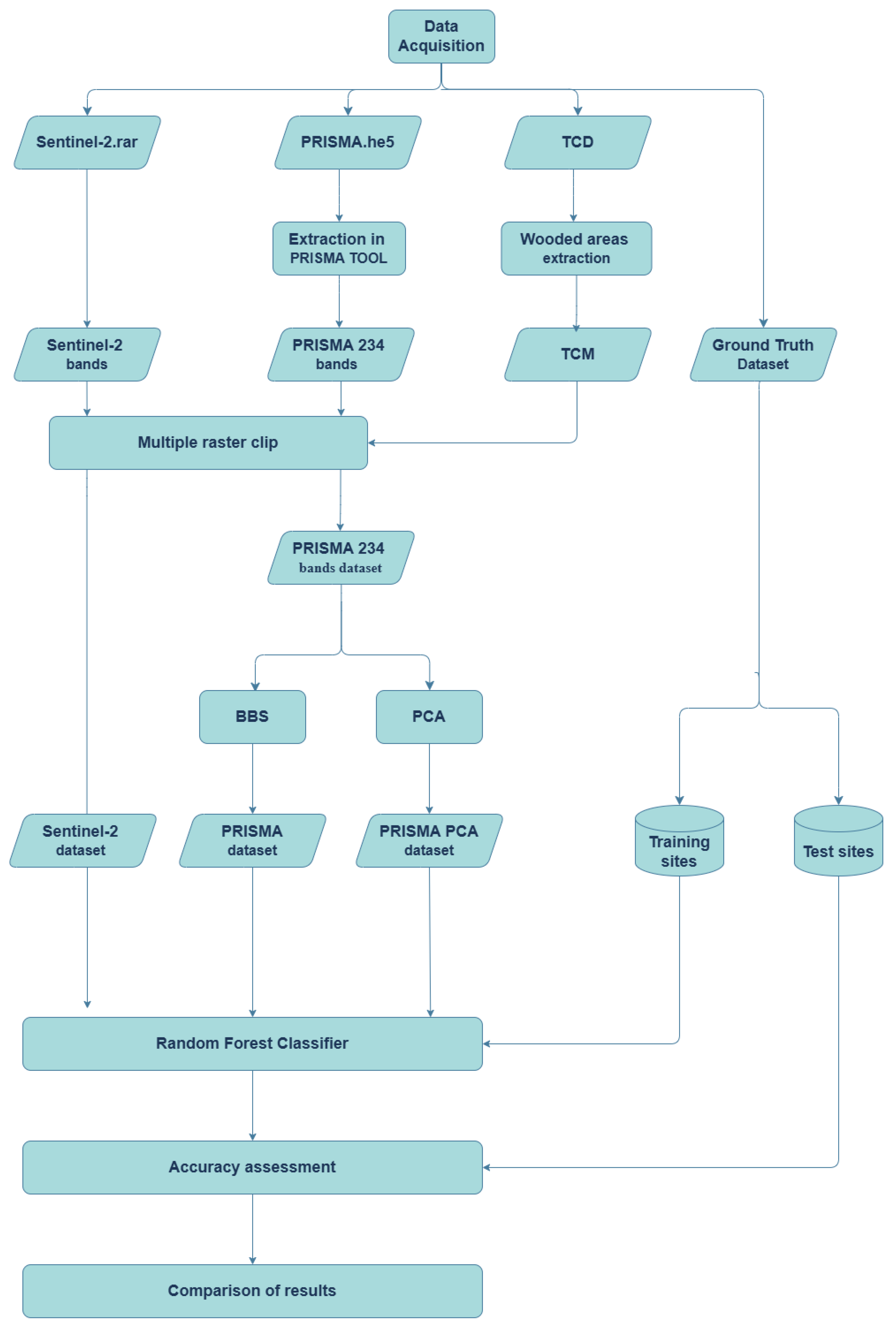
2.3.1. Workflow
2.3.2. Random Forest Classifier
2.4. Validation
3. Results
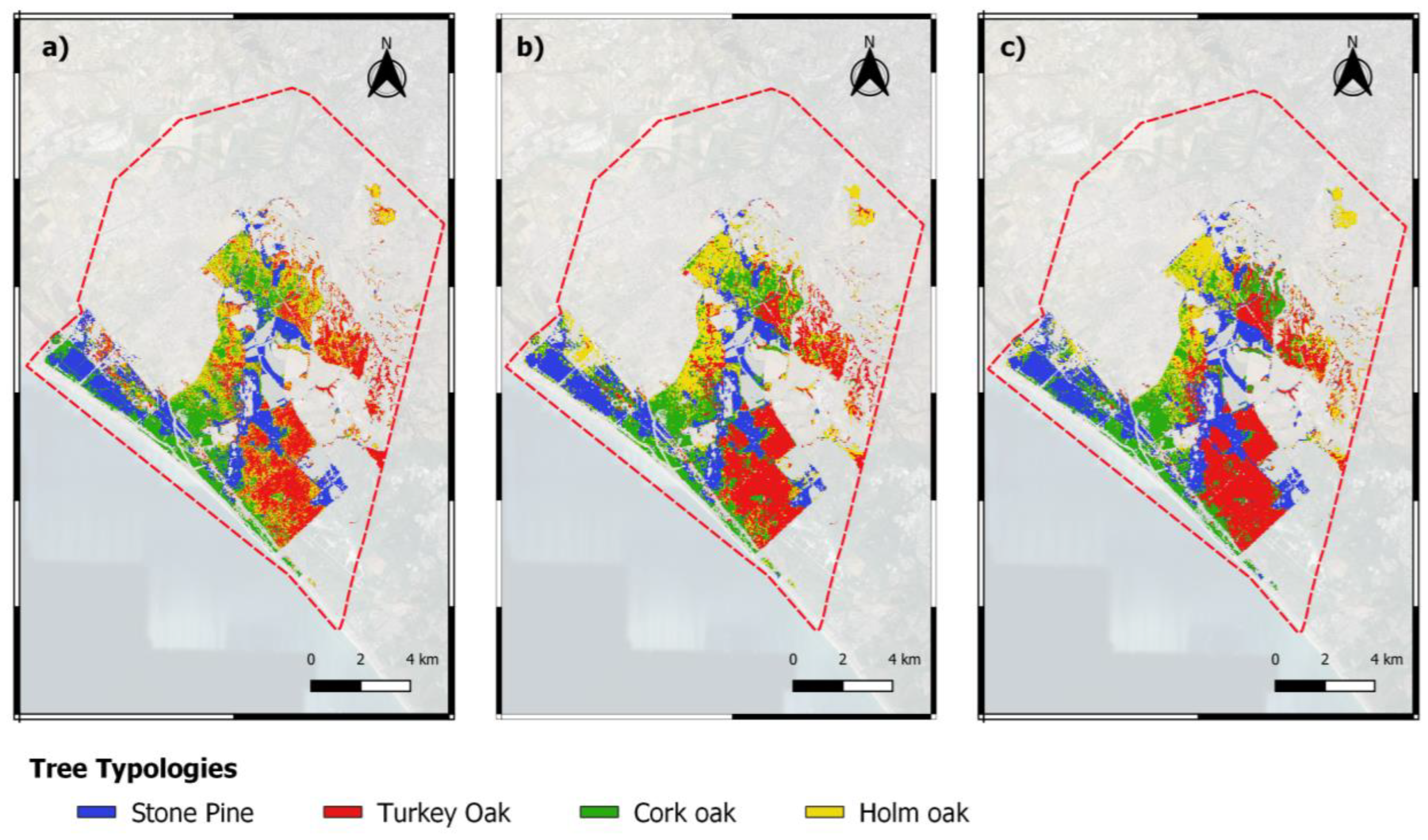
3.1. Roman Coastal
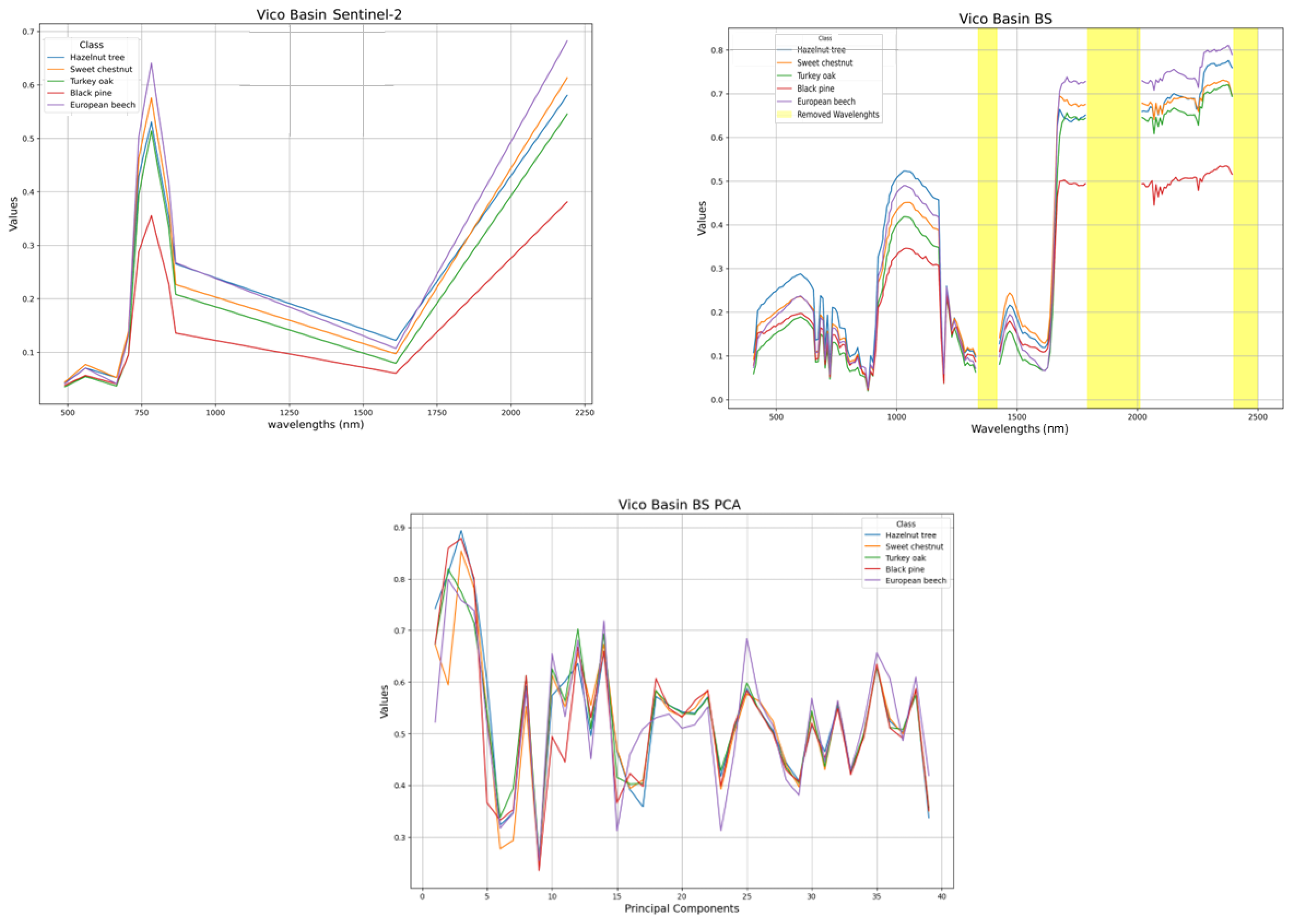
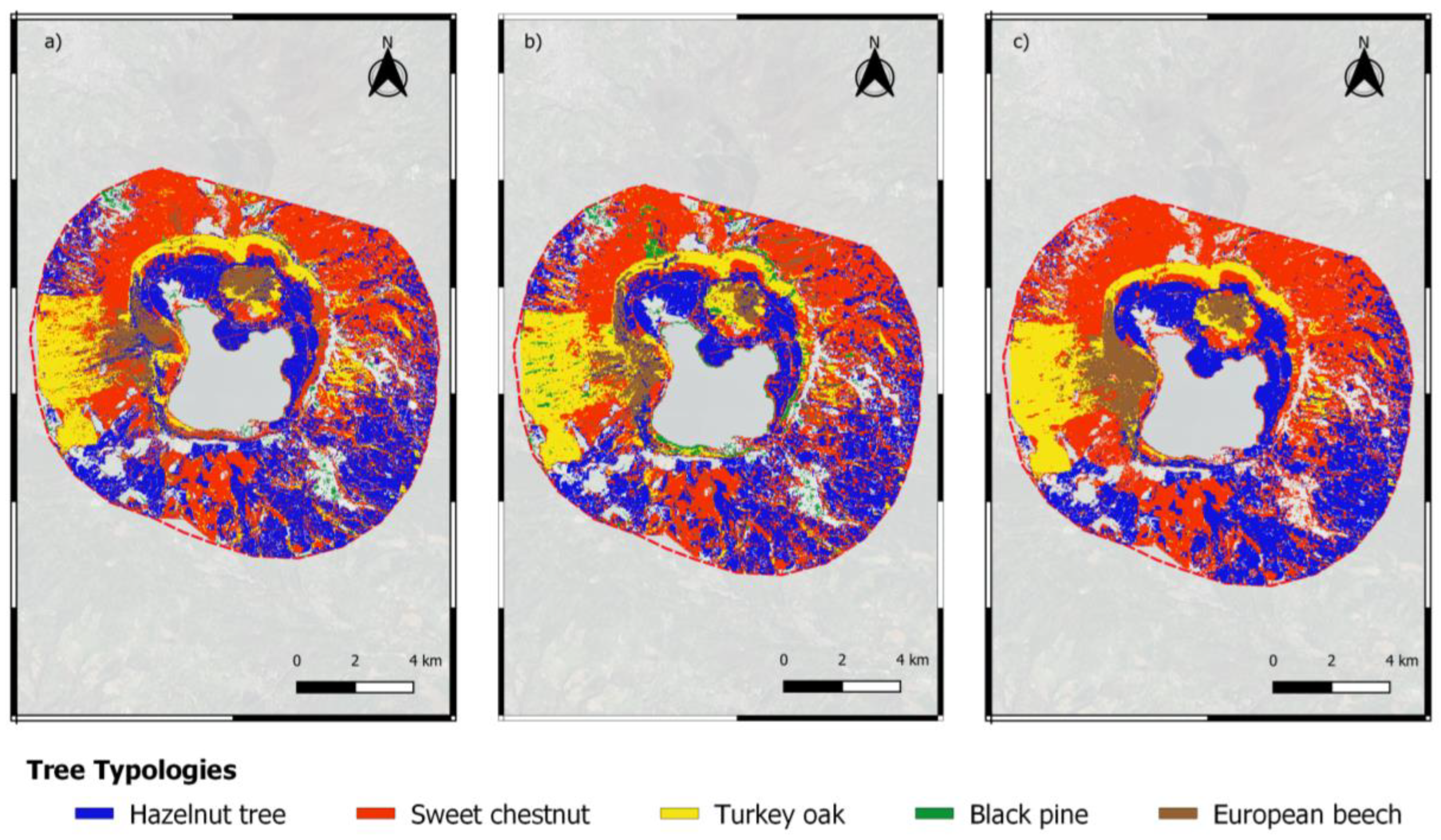
3.2. Lake Vico Basin Results
4. Discussion
5. Conclusions
Author Contributions
Funding
Data Availability Statement
Conflicts of Interest
References
- Giri, C.; Pengra, B.; Long, J.; Loveland, T.R. Next Generation of Global Land Cover Characterization, Mapping, and Monitoring. Int. J. Appl. Earth Obs. Geoinf. 2013, 25, 30–37. [Google Scholar] [CrossRef]
- Zhang, T.; Su, J.; Xu, Z.; Luo, Y.; Li, J. Sentinel-2 Satellite Imagery for Urban Land Cover Classification by Optimized Random Forest Classifier. Appl. Sci. 2021, 11, 543. [Google Scholar] [CrossRef]
- Lechner, A.M.; Foody, G.M.; Boyd, D.S. Applications in Remote Sensing to Forest Ecology and Management. One Earth 2020, 2, 405–412. [Google Scholar] [CrossRef]
- Skole, D.L.; Samek, J.H.; Dieng, M.; Mbow, C. The Contribution of Trees Outside of Forests to Landscape Carbon and Climate Change Mitigation in West Africa. Forests 2021, 12, 1652. [Google Scholar] [CrossRef]
- Patriarca, A.; Caputi, E.; Gatti, L.; Marcheggiani, E.; Recanatesi, F.; Rossi, C.M.; Ripa, M.N. Wide-Scale Identification of Small Woody Features of Landscape from Remote Sensing. Land 2024, 13, 1128. [Google Scholar] [CrossRef]
- Defries, R.S.; Townshend, J.R.G. Global Land Cover Characterization from Satellite Data: From Research to Operational Implementation? Glob. Ecol. Biogeogr. 1999, 8, 367–379. [Google Scholar] [CrossRef]
- Fassnacht, F.E.; White, J.C.; Wulder, M.A.; Næsset, E. Remote Sensing in Forestry: Current Challenges, Considerations and Directions. Forestry 2024, 97, 11–37. [Google Scholar] [CrossRef]
- Fassnacht, F.E.; Latifi, H.; Stereńczak, K.; Modzelewska, A.; Lefsky, M.; Waser, L.T.; Straub, C.; Ghosh, A. Review of Studies on Tree Species Classification from Remotely Sensed Data. Remote Sens. Environ. 2016, 186, 64–87. [Google Scholar] [CrossRef]
- Ørka, H.O.; Hansen, E.H.; Dalponte, M.; Gobakken, T.; Næsset, E. Large-Area Inventory of Species Composition Using Airborne Laser Scanning and Hyperspectral Data. Silva Fenn. 2021, 55, 10244. [Google Scholar] [CrossRef]
- Boyd, D.S.; Danson, F.M. Satellite Remote Sensing of Forest Resources: Three Decades of Research Development. Prog. Phys. Geogr. 2005, 29, 1–26. [Google Scholar] [CrossRef]
- Franklin, S.E.; Wulder, M.A. Remote Sensing Methods in Medium Spatial Resolution Satellite Data Land Cover Classification of Large Areas. Prog. Phys. Geogr. 2002, 26, 173–205. [Google Scholar] [CrossRef]
- Korhonen, L.; Hadi; Packalen, P.; Rautiainen, M. Comparison of Sentinel-2 and Landsat 8 in the Estimation of Boreal Forest Canopy Cover and Leaf Area Index. Remote Sens. Environ. 2017, 195, 259–274. [Google Scholar] [CrossRef]
- Astola, H.; Häme, T.; Sirro, L.; Molinier, M.; Kilpi, J. Comparison of Sentinel-2 and Landsat 8 Imagery for Forest Variable Prediction in Boreal Region. Remote Sens. Environ. 2019, 223, 257–273. [Google Scholar] [CrossRef]
- Loizzo, R.; Guarini, R.; Longo, F.; Scopa, T.; Formaro, R.; Facchinetti, C.; Varacalli, G. Prisma: The Italian Hyperspectral Mission. In Proceedings of the International Geoscience and Remote Sensing Symposium (IGARSS), Valencia, Spain, 22–27 July 2018; Volume 2018, pp. 175–178. [Google Scholar]
- Cogliati, S.; Sarti, F.; Chiarantini, L.; Cosi, M.; Lorusso, R.; Lopinto, E.; Miglietta, F.; Genesio, L.; Guanter, L.; Damm, A.; et al. The PRISMA Imaging Spectroscopy Mission: Overview and First Performance Analysis. Remote Sens. Environ. 2021, 262, 112499. [Google Scholar] [CrossRef]
- Storch, T.; Honold, H.-P.; Chabrillat, S.; Habermeyer, M.; Tucker, P.; Brell, M.; Ohndorf, A.; Wirth, K.; Betz, M.; Kuchler, M.; et al. The EnMAP Imaging Spectroscopy Mission towards Operations. Remote Sens. Environ. 2023, 294, 113632. [Google Scholar] [CrossRef]
- Grabska, E.; Frantz, D.; Ostapowicz, K. Evaluation of Machine Learning Algorithms for Forest Stand Species Mapping Using Sentinel-2 Imagery and Environmental Data in the Polish Carpathians. Remote Sens. Environ. 2020, 251, 112103. [Google Scholar] [CrossRef]
- Nomura, K.; Mitchard, E.T.A. More Than Meets the Eye: Using Sentinel-2 to Map Small Plantations in Complex Forest Landscapes. Remote Sens. 2018, 10, 1693. [Google Scholar] [CrossRef]
- Hościło, A.; Lewandowska, A. Mapping Forest Type and Tree Species on a Regional Scale Using Multi-Temporal Sentinel-2 Data. Remote Sens. 2019, 11, 929. [Google Scholar] [CrossRef]
- Persson, M.; Lindberg, E.; Reese, H. Tree Species Classification with Multi-Temporal Sentinel-2 Data. Remote Sens. 2018, 10, 1794. [Google Scholar] [CrossRef]
- Bolyn, C.; Michez, A.; Gaucher, P.; Lejeune, P.; Bonnet, S. Forest Mapping and Species Composition Using Supervised per Pixel Classification of Sentinel-2 Imagery|Cartographie Forestière et Composition Spécifique Par Classification Supervisée Par Pixel d’imagerie Sentinel-2. Biotechnol. Agron. Soc. Environ. 2018, 22, 172–187. [Google Scholar] [CrossRef]
- Puletti, N.; Chianucci, F.; Castaldi, C. Use of Sentinel-2 for Forest Classification in Mediterranean Environments. Ann. Silvic. Res. 2018, 42, 32–38. [Google Scholar] [CrossRef]
- Qiu, S.; He, B.; Yin, C.; Liao, Z. Assessments of Sentinel-2 Vegetation Red-Edge Spectral Bands for Improving Land Cover Classification. In Proceedings of the International Archives of the Photogrammetry, Remote Sensing and Spatial Information Sciences—ISPRS Archives, Wuhan, China, 18–22 September 2017; Volume 42, pp. 871–874. [Google Scholar]
- Amato, U.; Antoniadis, A.; Carfora, M.F.; Colandrea, P.; Cuomo, V.; Franzese, M.; Pignatti, S.; Serio, C. Statistical Classification for Assessing Prisma Hyperspectral Potential for Agricultural Land Use. IEEE J. Sel. Top. Appl. Earth Obs. Remote Sens. 2013, 6, 615–625. [Google Scholar] [CrossRef]
- Spiller, D.; Ansalone, L.; Carotenuto, F.; Mathieu, P.P. Crop Type Mapping Using Prisma Hyperspectral Images and One-Dimensional Convolutional Neural Network. In Proceedings of the International Geoscience and Remote Sensing Symposium (IGARSS), Brussels, Belgium, 11–16 July 2021; pp. 8166–8169. [Google Scholar]
- Vangi, E.; D’amico, G.; Francini, S.; Giannetti, F.; Lasserre, B.; Marchetti, M.; Chirici, G. The New Hyperspectral Satellite Prisma: Imagery for Forest Types Discrimination. Sensors 2021, 21, 1182. [Google Scholar] [CrossRef] [PubMed]
- Delogu, G.; Caputi, E.; Perretta, M.; Ripa, M.N.; Boccia, L. Using PRISMA Hyperspectral Data for Land Cover Classification with Artificial Intelligence Support. Sustainability 2023, 15, 13786. [Google Scholar] [CrossRef]
- Shaik, R.U.; Laneve, G.; Fusilli, L. An Automatic Procedure for Forest Fire Fuel Mapping Using Hyperspectral (PRISMA) Imagery: A Semi-Supervised Classification Approach. Remote Sens. 2022, 14, 1264. [Google Scholar] [CrossRef]
- Arasumani, M.; Thiel, F.; Pham, V.-D.; Hellmann, C.; Kaiser, M.; van der Linden, S. Advancing Peatland Vegetation Mapping by Spaceborne Imaging Spectroscopy. Ecol. Indic. 2023, 154, 110665. [Google Scholar] [CrossRef]
- Boggavarapu, L.N.P.; Prabukumar, M. Survey on Classification Methods for Hyper Spectral Remote Sensing Imagery. In Proceedings of the 2017 International Conference on Intelligent Computing and Control Systems, ICICCS 2017, Madurai, India, 15–16 June 2017; Volume 2018, pp. 538–542. [Google Scholar]
- Amini, S.; Saber, M.; Rabiei-Dastjerdi, H.; Homayouni, S. Urban Land Use and Land Cover Change Analysis Using Random Forest Classification of Landsat Time Series. Remote Sens. 2022, 14, 2654. [Google Scholar] [CrossRef]
- Belgiu, M.; Drăgu, L. Random Forest in Remote Sensing: A Review of Applications and Future Directions. ISPRS J. Photogramm. Remote Sens. 2016, 114, 24–31. [Google Scholar] [CrossRef]
- Sheykhmousa, M.; Mahdianpari, M.; Ghanbari, H.; Mohammadimanesh, F.; Ghamisi, P.; Homayouni, S. Support Vector Machine Versus Random Forest for Remote Sensing Image Classification: A Meta-Analysis and Systematic Review. IEEE J. Sel. Top. Appl. Earth Obs. Remote Sens. 2020, 13, 6308–6325. [Google Scholar] [CrossRef]
- Caputi, E.; Delogu, G.; Patriarca, A.; Perretta, M.; Gatti, L.; Boccia, L.; Ripa, M.N. Comparative Performance of Machine Learning Algorithms for Forest Cover Classification Using ASI—PRISMA Hyperspectral Data. In Proceedings of the 2023 IEEE International Workshop on Metrology for Agriculture and Forestry (MetroAgriFor), Pisa, Italy, 6–8 November 2023; pp. 248–252. [Google Scholar]
- Pelletier, C.; Valero, S.; Inglada, J.; Champion, N.; Dedieu, G. Assessing the Robustness of Random Forests to Map Land Cover with High Resolution Satellite Image Time Series over Large Areas. Remote Sens. Environ. 2016, 187, 156–168. [Google Scholar] [CrossRef]
- Rodriguez-Galiano, V.F.; Ghimire, B.; Rogan, J.; Chica-Olmo, M.; Rigol-Sanchez, J.P. An Assessment of the Effectiveness of a Random Forest Classifier for Land-Cover Classification. ISPRS J. Photogramm. Remote Sens. 2012, 67, 93–104. [Google Scholar] [CrossRef]
- Ahady, A.B.; Kaplan, G. Classification Comparison of Landsat-8 and Sentinel-2 Data in Google Earth Engine, Study Case of the City of Kabul. Int. J. Eng. Geosci. 2022, 7, 24–31. [Google Scholar] [CrossRef]
- Nasiri, V.; Deljouei, A.; Moradi, F.; Sadeghi, S.M.M.; Borz, S.A. Land Use and Land Cover Mapping Using Sentinel-2, Landsat-8 Satellite Images, and Google Earth Engine: A Comparison of Two Composition Methods. Remote Sens. 2022, 14, 1977. [Google Scholar] [CrossRef]
- Nasiri, V.; Beloiu, M.; Asghar Darvishsefat, A.; Griess, V.C.; Maftei, C.; Waser, L.T. Mapping Tree Species Composition in a Caspian Temperate Mixed Forest Based on Spectral-Temporal Metrics and Machine Learning. Int. J. Appl. Earth Obs. Geoinf. 2023, 116, 103154. [Google Scholar] [CrossRef]
- Awad, M.M. Forest Mapping: A Comparison between Hyperspectral and Multispectral Images and Technologies. J. Res. 2018, 29, 1395–1405. [Google Scholar] [CrossRef]
- Sedighi, A.; Hamzeh, S.; Firozjaei, M.K.; Goodarzi, H.V.; Naseri, A.A. Comparative Analysis of Multispectral and Hyperspectral Imagery for Mapping Sugarcane Varieties. PFG—J. Photogramm. Remote Sens. Geoinf. Sci. 2023, 91, 453–470. [Google Scholar] [CrossRef]
- Gancheva, I. Analysis of Hyperspectral and Multispectral Reflectance Spectra in the Black Sea Coastal Area near the Danube Delta: Comparison of PRISMA and Sentinel-2 Observations. J. Phys. Conf. Ser. 2022, 2255, 012015. [Google Scholar] [CrossRef]
- Goodenough, D.G.; Dyk, A.; Niemann, K.O.; Pearlman, J.S.; Chen, H.; Han, T.; Murdoch, M.; West, C. Processing Hyperion and ALI for Forest Classification. IEEE Trans. Geosci. Remote Sens. 2003, 41, 1321–1331. [Google Scholar] [CrossRef]
- Ferster, C.J.; Coops, N.C. Integrating Volunteered Smartphone Data with Multispectral Remote Sensing to Estimate Forest Fuels. Int. J. Digit. Earth 2016, 9, 171–196. [Google Scholar] [CrossRef]
- Chehdi, K.; Cariou, C. Learning or Assessment of Classification Algorithms Relying on Biased Ground Truth Data: What Interest? J. Appl. Remote Sens. 2019, 13, 1. [Google Scholar] [CrossRef]
- Manes, F.; Grignetti, A.; Tinelli, A.; Lenz, R.; Ciccioli, P. General Features of the Castelporziano Test Site. Atmos. Environ. 1997, 31, 19–25. [Google Scholar] [CrossRef]
- Recanatesi, F.; Giuliani, C.; Ripa, M.N. Monitoring Mediterranean Oak Decline in a Peri-Urban Protected Area Using the NDVI and Sentinel-2 Images: The Case Study of Castelporziano State Natural Reserve. Sustainability 2018, 10, 3308. [Google Scholar] [CrossRef]
- Recanatesi, F.; Giuliani, C.; Piccinno, M.; Cucca, B.; Rossi, C.M.; Ripa, M.N. An Innovative Environmental Risk Assessment Approach to a Mediterranean Coastal Forest: The Presidential Estate of Castelporziano (Rome) Case Study. Ann. Silvic. Res. 2020, 44, 80–85. [Google Scholar] [CrossRef]
- Recanatesi, F.; Ripa, M.N.; Leone, A.; Luigi, P.; Salvati, L. Land Use, Climate and Transport of Nutrients: Evidence Emerging from the Lake Vicocase Study. Environ. Manag. 2013, 52, 503–513. [Google Scholar] [CrossRef]
- Costantini, M.L.; Zaccarelli, N.; Mandrone, S.; Rossi, D.; Calizza, E.; Rossi, L. NDVI Spatial Pattern and the Potential Fragility of Mixed Forested Areas in Volcanic Lake Watersheds. Ecol. Manag. 2012, 285, 133–141. [Google Scholar] [CrossRef]
- ESA MSI Level-2A BOA Reflectance Product. Collection 1; European Space Agency: Paris, France, 2021.
- Sinha, P.; Kumar, L.; Reid, N. Seasonal Variation in Land-Cover Classification Accuracy in a Diverse Region. Photogramm. Eng. Remote Sens. 2012, 78, 271–280. [Google Scholar] [CrossRef]
- Baillarin, S.J.; Meygret, A.; Dechoz, C.; Petrucci, B.; Lacherade, S.; Tremas, T.; Isola, C.; Martimort, P.; Spoto, F. Sentinel-2 Level 1 Products and Image Processing Performances. In Proceedings of the 2012 IEEE International Geoscience and Remote Sensing Symposium, Munich, Germany, 22–27 July 2012; IEEE: New York, NY, USA, 2012; pp. 7003–7006. [Google Scholar]
- Guarini, R.; Loizzo, R.; Facchinetti, C.; Longo, F.; Ponticelli, B.; Faraci, M.; Dami, M.; Cosi, M.; Amoruso, L.; De Pasquale, V.; et al. PRISMA Hyperspectral Mission Products. In Proceedings of the International Geoscience and Remote Sensing Symposium (IGARSS), Valencia, Spain, 22–27 July 2018; Volume 2018, pp. 179–182. [Google Scholar]
- LarpUnina. Available online: https://Github.Com/LarpUnina/PrismaTool/Activity (accessed on 10 June 2024).
- QGIS Geographic Information System. QGIS Association. Available online: http://www.Qgis.Org (accessed on 21 November 2022).
- De Luca, G.; Carotenuto, F.; Genesio, L.; Pepe, M.; Toscano, P.; Boschetti, M.; Miglietta, F.; Gioli, B. Improving PRISMA Hyperspectral Spatial Resolution and Geolocation by Using Sentinel-2: Development and Test of an Operational Procedure in Urban and Rural Areas. ISPRS J. Photogramm. Remote Sens. 2024, 215, 112–135. [Google Scholar] [CrossRef]
- EyeLand App. 2024. Available online: https://Prineyeland.It/ (accessed on 10 November 2024).
- Nguyen, L.H.; Joshi, D.R.; Clay, D.E.; Henebry, G.M. Characterizing Land Cover/Land Use from Multiple Years of Landsat and MODIS Time Series: A Novel Approach Using Land Surface Phenology Modeling and Random Forest Classifier. Remote Sens. Environ. 2020, 238, 111017. [Google Scholar] [CrossRef]
- European Environment Agency. Available online: https://land.copernicus.eu/en/products/high-resolution-layer-tree-cover-density/tree-cover-density-2018 (accessed on 7 April 2024).
- Carfora, M.F.; Casa, R.; Laneve, G.; Mzid, N.; Pascucci, S.; Pignatti, S. Prisma Noise Coefficients Estimation. In Proceedings of the IGARSS 2022—2022 IEEE International Geoscience and Remote Sensing Symposium, Kuala Lumpur, Malaysia, 17–22 July 2022; pp. 7531–7534. [Google Scholar]
- Lyngdoh, R.B.; Sahadevan, A.S.; Ahmad, T.; Rathore, P.S.; Mishra, M.; Gupta, P.K.; Misra, A. AVHYAS: A Free and Open Source QGIS Plugin for Advanced Hyperspectral Image Analysis. In Proceedings of the 2021 International Conference on Emerging Techniques in Computational Intelligence, ICETCI 2021, Hyderabad, India, 25–27 August 2021; pp. 71–76. [Google Scholar]
- Sawant, S.S.; Prabukumar, M. A Survey of Band Selection Techniques for Hyperspectral Image Classification. J. Spectr. Imaging 2020, 9, a5. [Google Scholar] [CrossRef]
- Marzialetti, F.; Cascone, S.; Frate, L.; Di Febbraro, M.; Acosta, A.T.R.; Carranza, M.L. Measuring Alpha and Beta Diversity by Field and Remote-Sensing Data: A Challenge for Coastal Dunes Biodiversity Monitoring. Remote Sens. 2021, 13, 1928. [Google Scholar] [CrossRef]
- Congedo, L. Semi-Automatic Classification Plugin: A Python Tool for the Download and Processing of Remote Sensing Images in QGIS. J. Open Source Softw. 2021, 6, 3172. [Google Scholar] [CrossRef]
- Breiman, L. Random Forests. Mach. Learn. 2001, 45, 5–32. [Google Scholar] [CrossRef]
- Noi, P.T.; Kappas, M. Comparison of Random Forest, k-Nearest Neighbor, and Support Vector Machine Classifiers for Land Cover Classification Using Sentinel-2 Imagery. Sensors 2018, 18, 18. [Google Scholar] [CrossRef]
- Naidu, G.; Zuva, T.; Sibanda, E.M. A Review of Evaluation Metrics in Machine Learning Algorithms. In Computer Science On-line Conference; Springer International Publishing: Cham, Switzerland, 2023; Volume 724 LNNS, ISBN 9783031353130. [Google Scholar]
- Congalton, R.G.; Green, K. Assessing the Accuracy of Remotely Sensed Data: Principles and Practices, 2nd ed.; CRC Press: Boca Raton, FL, USA, 2008; ISBN 9781420055139. [Google Scholar]
- Mallinis, G.; Galidaki, G.; Gitas, I. A Comparative Analysis of EO-1 Hyperion, Quickbird and Landsat TM Imagery for Fuel Type Mapping of a Typical Mediterranean Landscape. Remote Sens. 2014, 6, 1684–1704. [Google Scholar] [CrossRef]
- Foody, G.M. Thematic Map Comparison. Photogramm. Eng. Remote Sens. 2004, 70, 627–633. [Google Scholar] [CrossRef]
- Congalton, R.G. Accuracy Assessment and Validation of Remotely Sensed and Other Spatial Information. Int. J. Wildland Fire 2001, 10, 321–328. [Google Scholar] [CrossRef]
- Yel, S.G.; Tunc Gormus, E. Exploiting Hyperspectral and Multispectral Images in the Detection of Tree Species: A Review. Front. Remote Sens. 2023, 4, 1136289. [Google Scholar] [CrossRef]
- Delogu, G.; Perretta, M.; Caputi, E.; Patriarca, A.; Funsten, C.C.; Recanatesi, F.; Ripa, M.N.; Boccia, L. Leveraging the Potential of PRISMA Hyperspectral Data for Forest Tree Species Classification: A Case Study in Southern Italy. Remote Sens. 2024, 16, 4788. [Google Scholar] [CrossRef]
- George, R.; Padalia, H.; Kushwaha, S.P.S. Forest Tree Species Discrimination in Western Himalaya Using EO-1 Hyperion. Int. J. Appl. Earth Obs. Geoinf. 2014, 28, 140–149. [Google Scholar] [CrossRef]
- Puletti, N.; Camarretta, N.; Corona, P. Evaluating EO1-Hyperion Capability for Mapping Conifer and Broadleaved Forests. Eur. J. Remote Sens. 2016, 49, 157–169. [Google Scholar] [CrossRef]
- Lim, J.; Kim, K.-M.; Jin, R. Tree Species Classification Using Hyperion and Sentinel-2 Data with Machine Learning in South Korea and China. ISPRS Int. J. Geoinf. 2019, 8, 150. [Google Scholar] [CrossRef]
- Kluczek, M.; Zagajewski, B.; Zwijacz-Kozica, T. Mountain Tree Species Mapping Using Sentinel-2, PlanetScope, and Airborne HySpex Hyperspectral Imagery. Remote Sens. 2023, 15, 844. [Google Scholar] [CrossRef]
- Arfa, A.; Minaei, M. Utilizing Multitemporal Indices and Spectral Bands of Sentinel-2 to Enhance Land Use and Land Cover Classification with Random Forest and Support Vector Machine. Adv. Space Res. 2024, 74, 5580–5590. [Google Scholar] [CrossRef]
- Perretta, M.; Delogu, G.; Funsten, C.; Patriarca, A.; Caputi, E.; Boccia, L. Testing the Impact of Pansharpening Using PRISMA Hyperspectral Data: A Case Study Classifying Urban Trees in Naples, Italy. Remote Sens. 2024, 16, 3730. [Google Scholar] [CrossRef]
- Alparone, L.; Arienzo, A.; Garzelli, A. Spatial Resolution Enhancement of Satellite Hyperspectral Data via Nested Hypersharpening With Sentinel-2 Multispectral Data. IEEE J. Sel. Top. Appl. Earth Obs. Remote Sens. 2024, 17, 10956–10966. [Google Scholar] [CrossRef]


| (a) | |||||
| Tree Types Classes | Tree Species | ID | N° PRISMA Training Polygons | N° Sentinel-2 Training Polygons | Number of Test Sites |
| Stone Pine | Pinus pinea | 1 | 40 | 139 | 122 |
| Turkey Oak | Quercus cerris | 2 | 104 | 387 | 197 |
| Cork oak | Quercus suber | 3 | 65 | 232 | 44 |
| Holm oak | Quercus ilex | 4 | 62 | 224 | 56 |
| (b) | |||||
| Tree Types Classes | Tree Species | ID | N° PRISMA Training Polygons | N° Sentinel-2 Training Polygons | Number of Test Sites |
| Hazelnut tree | Corylus avellana | 1 | 197 | 708 | 178 |
| Sweet Chestnut | Castanea sativa | 2 | 138 | 529 | 132 |
| Turkey Oak | Quercus cerris | 3 | 78 | 265 | 85 |
| Black Pine | Pinus nigra | 4 | 13 | 52 | 4 |
| European Beech | Fagus sylvatica | 5 | 47 | 180 | 29 |
| Parameter | Value |
|---|---|
| n_estimators | 100 |
| criterion | Gini |
| bootstrap | True |
| min_samples_split | 2 |
| min_samples_leaf | 1 |
| min_weight_fraction_leaf | 0.00 |
| max_features | Auto |
| max_leaf_node | 0 |
| min_impurity_decrease | 0.00 |
| min_impurity_split | 0 |
| max_depth | True |
| n_jobs | −1 |
| training sample size | 80% |
| Roman Coastal | Lake Vico Basin | |||||||
|---|---|---|---|---|---|---|---|---|
| OA% | WiOA% | K | Z-Test | OA% | WiOA% | K | Z-Test | |
| Sentinel-2 | 64.54 | 68.20 | 0.51 | 9.49 | 78.97 | 78.85 | 0.64 | 9.70 |
| PRISMA BSD | 67.77 | 70.33 | 0.55 | 10.28 | 80.14 | 80.98 | 0.54 | 5.07 |
| PRISMA PCA | 71.09 | 72.74 | 0.59 | 11.50 | 87.15 | 87.33 | 0.77 | 14.34 |
| Z-Test Roman Coastal | ||
|---|---|---|
| PRISMA BSD | PRISMA PCA | |
| Z-Statistic | Z-Statistic | |
| Sentinel-2 | −0.49 | −1.08 |
| PRISMA PCA | −0.58 | |
| Z-Test Lake Vico Basin | ||
|---|---|---|
| PRISMA BSD | PRISMA PCA | |
| Z-Statistic | Z-Statistic | |
| Sentinel-2 | 0.80 | −1.58 |
| PRISMA PCA | −1.97 | |
| McNemar Roman Coastal | ||||
|---|---|---|---|---|
| PRISMA BSD | PRISMA PCA | |||
| p-value | X2 | p-value | X2 | |
| Sentinel-2 | 0.48 | 0.62 | 0.014 | 6.5 |
| PRISMA PCA | 0.02 | 6.0 | ||
| McNemar Lake Vico Basin | ||||
|---|---|---|---|---|
| PRISMA BSD | PRISMA PCA | |||
| p-value | X2 | p-value | X2 | |
| Sentinel-2 | 0.69 | 0.24 | 0.00002 | 18.5 |
| PRISMA PCA | 0.0001 | 14.9 | ||
| BCS Roman Coastal | |||
|---|---|---|---|
| Sentinel_2 | PRISMA_BS | PRISMA_BS_PCA | |
| Stone pine–Turkey oak | 0.75 | 0.72 | 0.37 |
| Stone pine–Cork oak | 0.77 | 0.75 | 0.41 |
| Stone pine–Holm oak | 0.77 | 0.75 | 0.40 |
| Turkey oak–Cork oak | 0.97 | 0.95 | 0.91 |
| Turkey oak–Holm oak | 0.96 | 0.94 | 0.90 |
| Cork oak–Holm oak | 0.99 | 0.98 | 0.96 |
| Roman Coastal Accuracy Metrics | |||||||||
|---|---|---|---|---|---|---|---|---|---|
| Tree Typologies | Sentinel-2 | PRISMA BSD | PRISMA PCA | ||||||
| PA (%) | UA (%) | F1 (%) | PA (%) | UA (%) | F1 (%) | PA (%) | UA (%) | F1 (%) | |
| Stone Pine | 76.23 | 90.29 | 82.67 | 79.51 | 88.18 | 83.62 | 87.70 | 86.99 | 87.35 |
| Turkey Oak | 58.21 | 92.13 | 71.34 | 61.50 | 91.11 | 73.43 | 61.50 | 92.48 | 73.87 |
| Holm Oak | 61.36 | 25.00 | 35.53 | 70.45 | 33.33 | 45.26 | 77.27 | 39.53 | 52.31 |
| Cork Oak | 64.29 | 42.35 | 51.06 | 62.50 | 41.67 | 50.00 | 64.29 | 45.00 | 52.94 |
| BCS Lake Vico Basin | |||
|---|---|---|---|
| Sentinel_2 | PRISMA_BS | PRISMA_BS_PCA | |
| Hazelnut tree—Sweet chestnut | 0.95 | 0.96 | 0.80 |
| Hazelnut tree—Turkey oak | 0.93 | 0.93 | 0.73 |
| Hazelnut tree—Black pine | 0.78 | 0.83 | 0.16 |
| Hazelnut tree—European beech | 0.93 | 0.94 | 0.80 |
| Sweet chestnut—Turkey oak | 0.92 | 0.95 | 0.79 |
| Sweet chestnut—Black pine | 0.77 | 0.85 | 0.32 |
| Sweet chestnut—European beech | 0.94 | 0.95 | 0.79 |
| Turkey oak—Black pine | 0.83 | 0.88 | 0.25 |
| Turkey oak—European beech | 0.88 | 0.92 | 0.79 |
| Black pine—European beech | 0.73 | 0.82 | 0.21 |
| Lake Vico Basin Accuracy Metrics | |||||||||
|---|---|---|---|---|---|---|---|---|---|
| Tree Typologies | Sentinel-2 | PRISMA BSD | PRISMA PCA | ||||||
| PA (%) | UA (%) | F1 (%) | PA (%) | UA (%) | F1 (%) | PA (%) | UA (%) | F1 (%) | |
| Hazelnut Tree | 87.08 | 86.11 | 86.59 | 82.58 | 88.55 | 85.47 | 88.76 | 94.61 | 91.59 |
| Sweet Chestnut | 80.3 | 73.61 | 76.81 | 78.79 | 74.82 | 76.75 | 90.91 | 78.95 | 84.51 |
| Turkey Oak | 69.41 | 79.73 | 74.21 | 83.53 | 87.65 | 85.54 | 78.82 | 94.37 | 85.9 |
| Black Pine | 75.00 | 42.86 | 54.55 | 75.00 | 17.65 | 28.57 | 75.00 | 50.00 | 60.00 |
| European Beech | 51.72 | 65.22 | 57.69 | 62.07 | 72.00 | 66.67 | 86.21 | 78.13 | 81.97 |
Disclaimer/Publisher’s Note: The statements, opinions and data contained in all publications are solely those of the individual author(s) and contributor(s) and not of MDPI and/or the editor(s). MDPI and/or the editor(s) disclaim responsibility for any injury to people or property resulting from any ideas, methods, instructions or products referred to in the content. |
© 2025 by the authors. Licensee MDPI, Basel, Switzerland. This article is an open access article distributed under the terms and conditions of the Creative Commons Attribution (CC BY) license (https://creativecommons.org/licenses/by/4.0/).
Share and Cite
Caputi, E.; Delogu, G.; Patriarca, A.; Perretta, M.; Mancini, G.; Boccia, L.; Recanatesi, F.; Ripa, M.N. Comparison of Tree Typologies Mapping Using Random Forest Classifier Algorithm of PRISMA and Sentinel-2 Products in Different Areas of Central Italy. Remote Sens. 2025, 17, 356. https://doi.org/10.3390/rs17030356
Caputi E, Delogu G, Patriarca A, Perretta M, Mancini G, Boccia L, Recanatesi F, Ripa MN. Comparison of Tree Typologies Mapping Using Random Forest Classifier Algorithm of PRISMA and Sentinel-2 Products in Different Areas of Central Italy. Remote Sensing. 2025; 17(3):356. https://doi.org/10.3390/rs17030356
Chicago/Turabian StyleCaputi, Eros, Gabriele Delogu, Alessio Patriarca, Miriam Perretta, Giulia Mancini, Lorenzo Boccia, Fabio Recanatesi, and Maria Nicolina Ripa. 2025. "Comparison of Tree Typologies Mapping Using Random Forest Classifier Algorithm of PRISMA and Sentinel-2 Products in Different Areas of Central Italy" Remote Sensing 17, no. 3: 356. https://doi.org/10.3390/rs17030356
APA StyleCaputi, E., Delogu, G., Patriarca, A., Perretta, M., Mancini, G., Boccia, L., Recanatesi, F., & Ripa, M. N. (2025). Comparison of Tree Typologies Mapping Using Random Forest Classifier Algorithm of PRISMA and Sentinel-2 Products in Different Areas of Central Italy. Remote Sensing, 17(3), 356. https://doi.org/10.3390/rs17030356