Improved Stereophotogrammetric and Multi-View Shape-from-Shading DTMs of Occator Crater and Its Interior Cryovolcanism-Related Bright Spots

Abstract

Over the course of NASA’s Dawn Discovery mission, the onboard framing camera mapped Ceres across a wide wavelength spectrum at varying polar science orbits and altitudes. With increasing resolution, the uniqueness of the 92 km wide, young Occator crater became evident. Its central cryovolcanic dome, Cerealia Tholus, and especially the associated bright carbonate and ammonium chloride deposits—named Cerealia Facula and the thinner, more dispersed Vinalia Faculae—are the surface expressions of a deep brine reservoir beneath Occator. Understandably, this made this crater the target for future sample return mission studies. The planning and preparation for this kind of mission require the characterization of potential landing sites based on the most accurate topography and orthorectified image data. In this work, we demonstrate the capabilities of the freely available and open-source USGS Integrated Software for Imagers and Spectrometers (ISIS 3) and Ames Stereo Pipeline (ASP 2.7) in creating high-quality image data products as well as stereophotogrammetric (SPG) and multi-view shape-from-shading (SfS) digital terrain models (DTMs) of the aforementioned spectroscopically challenging features. The main data products of our work are four new DTMs, including one SPG and one SfS DTM based on High-Altitude Mapping Orbit (HAMO) (CSH/CXJ) and one SPG and one SfS DTM based on Low-Altitude Mapping Orbit (LAMO) (CSL/CXL), along with selected Extended Mission Orbit 7 (XMO7) framing camera (FC) data. The SPG and SfS DTMs were calculated to a GSD of 1 and 0.5 px, corresponding to 136 m (HAMO SPG), 68 m (HAMO SfS), 34 m (LAMO SPG), and 17 m (LAMO SfS). Finally, we show that the SPG and SfS approaches we used yield consistent results even in the presence of high albedo differences and highlight how our new DTMs differ from those previously created and published by the German Aerospace Center (DLR) and the Jet Propulsion Laboratory (JPL).

1. Introduction

With the detection of subsurface oceans beneath the icy crusts of several Jovian and Saturnian moons by the Galileo and Cassini spacecraft, it became evident that the search for extraterrestrial life must extend beyond the traditional habitable zone. To date, evidence of subsurface oceans has been identified on five moons—Europa [1,2,3,4,5,6,7], Enceladus [8,9,10,11,12,13], Titan [14,15,16], Ganymede [17], and Callisto [3,4,5]—through the analysis of gravity, shape, libration, and radio Doppler data, the detection of induced magnetic fields and their perturbations, observations of plumes, the chemical analysis of ejected particles, and geomorphological studies of their surfaces. Among these five confirmed ocean worlds, Europa, Enceladus, and Titan are considered the highest priority targets in NASA’s Roadmap to Ocean Worlds (ROWs) [18]. Additionally, a group of objects showing less definitive evidence but some indications of extant subsurface liquids have been classified as potential or candidate ocean worlds. This group includes Saturn’s moon Dione [10], Neptune’s moon Triton [19], Pluto [20,21], and the dwarf planet Ceres [22].

Among the confirmed and candidate ocean worlds, Ceres occupies a unique position for two reasons. First, it may represent an end-member in terms of its physical properties (e.g., size, density, heat budget), and second, it is the only icy body that has been extensively mapped by an orbiter mission [23]. Recent findings by the Dawn Science Team [24,25,26,27,28,29,30,31] indicate that Ceres shares certain characteristics with ocean worlds while also exhibiting significant differences. Without a substantial internal heat source or tidal heating to sustain large amounts of liquid water, much of Ceres’ subsurface water has frozen [32], leaving behind a relict ocean world with a volatile-rich crust [33,34,35,36,37] and possibly scattered subsurface brine reservoirs [28,38]. The most prominent surface manifestations of these brine reservoirs have been found within the fresh 92 km Occator crater (Figure 1), in the form of a central cryovolcanic dome called the Cerealia Tholus (CT) and the surrounding bright deposits known as the Cerealia Facula (CF) (see Figure 2). These deposits are rich in carbonates [24,25,39] and ammonium chloride [24], while several other dispersed, thin bright deposits named the Vinalia Faculae (VF) are thought to have formed through more explosive mechanisms [40]. Unsurprisingly, the Occator crater has been a focal point in Ceres’ landing site assessments [41] and is the target of mission concept studies and sample return missions [42,43,44] aimed at probing the evaporites originating from the 50 km deep brine reservoir beneath it [28,31].

To further investigate Ceres’ potential habitability, future in situ missions represent the next logical step [45]. The planning and preparation of landing or sample return missions (e.g., [43]) require a detailed characterization of potential landing sites based on the most accurate topography and orthorectified image data [46]. The Occator crater, our primary investigation area, is characterized by very large albedo variations (of as much as a factor of 10) that present significant challenges for topographic reconstruction (see Section 2.4). At the same time, these enable a far more demanding test of the SfS method with albedo modeling than most other studies, which generally consider only fractional or at most factor-of-two differences in the albedo. In this work, we present the first two steps: the production of stereophotogrammetrically (SPG) and multi-view shape-from-shading (simply abbreviated as SfS in our study)-derived digital terrain models (DTMs) and controlled, bundle-adjusted, photometrically corrected orthorectified image data and mosaics. These steps are necessary to create matching framing camera (FC) [47] color cubes, slope maps, and other higher level data products such as pan-sharpened high-resolution color data, which will form the basis for processing the very high-resolution data acquired during Dawn’s second extended mission phase (XM2). We also highlight the benefits and, indeed, the necessity of using high-resolution DTMs for accurate photometric corrections, particularly for narrow-band filters and their effects on color composites. Our entire workflow was implemented using the freely available USGS Integrated Software for Imagers and Spectrometers 3 (now in version 8.2.0 https://isis.astrogeology.usgs.gov/8.2.0/, accessed on 23 Decemeber 2024) (ISIS 3) and the Ames Stereo Pipeline (https://stereopipeline.readthedocs.io/en/latest/news.html#release-2-7-0-july-27-2020, accessed on 23 Decemeber 2024) (ASP 2.7) [48,49]. In our study, we utilized the ASP 2.7 to generate DTMs based on SPG and SfS. The algorithms implemented in the ASP 2.7 operate independently of, and differ significantly from, the software used in previous studies conducted by the DLR and the JPL. This independence ensures methodological diversity and provides an opportunity to validate and complement earlier results through an entirely distinct computational framework. Our complete workflow involving the ISIS 3 and the ASP 2.7 is described in detail in Section 4 for reproducibility.

2. Background

The Dawn spacecraft [50] is equipped with three scientific instruments: two identical framing cameras (FC1 and FC2) [47], a visual and infrared spectrometer (VIR) [51], and a gamma ray and neutron detector (GRaND) [52]. Also, the telecom subsystem is used for gravity science [53]. As our current work focuses exclusively on imaging data, the following subsections are limited to describing the FC, the ground resolution achieved across various orbits (Table 1), and the derived data products, such as DTMs and the related orthomosaics, produced from FC data that are currently published and archived (see Table 2).

2.1. Dawn Mission Overview

During the 46-month active mission at Ceres, ending in late October 2018, the Dawn spacecraft globally mapped the dwarf planet from various altitudes, achieving a range of ground resolutions. Following the Approach and Rotation Calibration (RC3) phase, Dawn entered a series of stable polar orbits with decreasing altitudes, enabling data acquisition at consistent ground resolutions during each mission phase. As with the mission plan for Vesta [54], a key objective was to achieve near-global, multi-temporal coverage of Ceres using the FC F1CLEAR filter during the Ceres Science Survey (CSS), CSH, and CSL phases. These orbits provided median GSDs of 410.6 m, 138.0 m, and 36.1 m, respectively, suitable for generating stereophotogrammetric DTMs and the corresponding orthomosaics. This dataset was further extended during the first extended mission (XM1), specifically in the Ceres Extended LAMO (CXL) and Ceres Extended Juling (CXJ) phases. Additionally, global mapping was performed using seven narrow-band filters (F2–F8) [47] during the CSS and CSH/CXJ phases, allowing for the creation of multispectral color cubes and global color mosaics. A comprehensive overview of the different mission phases at Ceres, including altitudes, ground resolutions, and the number of acquired images, is provided in Table 1 and Figure 3.

Table 1. Mission phases, orbits, and related metadata. For each orbit phase, we calculated the minimum, median, and maximum values for the orbit radii, height or distance between the spacecraft and the surface, and the ground sample distance (GSD).

Orbit Phase	ID	Orbit	Start	Orbit Radii (km)			Height (km)			GSD (m)
				Min.	Mdn.	Max.	Min.	Mdn.	Max.	Min.	Mdn.	Max.
Vesta–Ceres Cruise	VCC		2012/09/10
Ceres Science Approach	CSA		2015/01/13
Ceres Science RC3	CSR		2015/04/25	13,963	14,012	14,104	13,493	13,568	13,996	1258.7	1265.6	1305.0
Ceres Transfer to Survey	CTS		2015/05/16	5545	5575	7771	5079	5126	7310	473.8	478.4	681.9
Ceres Science Survey	CSS		2015/06/05	4854	4863	4870	4379	4402	4575	407.7	410.6	426.7
Ceres Transfer To HAMO	CTH		2015/07/01
Ceres Science HAMO	CSH		2015/08/18	1932	1940	1945	1456	1480	1602	135.6	138.0	149.5
Ceres Transfer to LAMO	CTL		2015/10/23
Ceres Science LAMO	CSL		2015/12/16	839	848	861	388	386.9	615	33.0	36.1	57.4
End of Dawn’s primary mission at Ceres
Ceres Extended LAMO	CXL	XMO1	2016/06/19	836	849	861	357	392	693	33.3	36.5	64.7
Ceres Transfer to Juling	CTJ		2016/09/02
Ceres Extended Juling	CXJ	XMO2	2016/10/17	1930	1961	1965	1476	1489	1734	137.4	138.9	161.7
Ceres Transfer of GRaND	CTG		2016/11/03
Ceres Extended GRaND	CXG	XMO3	2017/01/27	8014	8024	8197	7580	7653	7812	705.7	713.7	729.9
Ceres Transfer to Opposition	CTO		2017/02/23
Ceres Extended Opposition	CXO	XMO4	2017/03/28	19,267	20,457	48,876	18,837	19,998	48,629	1757.2	1865.6	4536.4
End of Dawn’s first extended mission (XM1) at Ceres
Extended Mission Orbit 5		XMO5	2017/07/01
Transfer to Extended Mission Orbit 6			2018/04/16
Extended Mission Orbit 6		XMO6	2018/05/16	911	982	3508	451	537	3059	41.9	50.1	285.4
Transfer to Extended Mission Orbit 7			2018/05/31
Extended Mission Orbit 7		XMO7	2018/06/09	503	529	4458	29	57	4297	2.7	5.3	400.9

Table 1. Mission phases, orbits, and related metadata. For each orbit phase, we calculated the minimum, median, and maximum values for the orbit radii, height or distance between the spacecraft and the surface, and the ground sample distance (GSD).

Orbit Phase	ID	Orbit	Start	Orbit Radii (km)			Height (km)			GSD (m)
				Min.	Mdn.	Max.	Min.	Mdn.	Max.	Min.	Mdn.	Max.
Vesta–Ceres Cruise	VCC		2012/09/10
Ceres Science Approach	CSA		2015/01/13
Ceres Science RC3	CSR		2015/04/25	13,963	14,012	14,104	13,493	13,568	13,996	1258.7	1265.6	1305.0
Ceres Transfer to Survey	CTS		2015/05/16	5545	5575	7771	5079	5126	7310	473.8	478.4	681.9
Ceres Science Survey	CSS		2015/06/05	4854	4863	4870	4379	4402	4575	407.7	410.6	426.7
Ceres Transfer To HAMO	CTH		2015/07/01
Ceres Science HAMO	CSH		2015/08/18	1932	1940	1945	1456	1480	1602	135.6	138.0	149.5
Ceres Transfer to LAMO	CTL		2015/10/23
Ceres Science LAMO	CSL		2015/12/16	839	848	861	388	386.9	615	33.0	36.1	57.4
End of Dawn’s primary mission at Ceres
Ceres Extended LAMO	CXL	XMO1	2016/06/19	836	849	861	357	392	693	33.3	36.5	64.7
Ceres Transfer to Juling	CTJ		2016/09/02
Ceres Extended Juling	CXJ	XMO2	2016/10/17	1930	1961	1965	1476	1489	1734	137.4	138.9	161.7
Ceres Transfer of GRaND	CTG		2016/11/03
Ceres Extended GRaND	CXG	XMO3	2017/01/27	8014	8024	8197	7580	7653	7812	705.7	713.7	729.9
Ceres Transfer to Opposition	CTO		2017/02/23
Ceres Extended Opposition	CXO	XMO4	2017/03/28	19,267	20,457	48,876	18,837	19,998	48,629	1757.2	1865.6	4536.4
End of Dawn’s first extended mission (XM1) at Ceres
Extended Mission Orbit 5		XMO5	2017/07/01
Transfer to Extended Mission Orbit 6			2018/04/16
Extended Mission Orbit 6		XMO6	2018/05/16	911	982	3508	451	537	3059	41.9	50.1	285.4
Transfer to Extended Mission Orbit 7			2018/05/31
Extended Mission Orbit 7		XMO7	2018/06/09	503	529	4458	29	57	4297	2.7	5.3	400.9

2.2. The Dawn Framing Camera (FC)

As the framing camera (FC) was not only crucial for various scientific objectives but also served as an optical navigation system [47,54], the Dawn spacecraft was equipped with two identical and fully independent cameras for redundancy. While the majority of the FC data were acquired by the primary camera (FC2), the secondary or backup camera (FC1) was primarily used to capture simultaneous images to increase the spatial coverage during the time-limited second extended mission (XM2) phase, specifically during the seventh extended mission orbit (XMO7). In addition to the wide-band F1CLEAR filter, which was employed for most of the data acquisition, the FC was equipped with seven narrow-band filters. Among them, the F7RED (650 nm), F2GREEN (550 nm), F8BLUE (430 nm), and F5IR (980 nm) filters were used for spectral analyses and for collecting color data to generate RGB or IRGB color composites. Two examples of photometrically corrected IRGB color composite mosaics are shown in Figure 1 and Figure 2. The remaining three near-infrared filters (F3, F4, and F6) were utilized in this work solely for the identification of defective pixels on the CCD chip (see Figure 4).

2.3. Currently Published and Archived DTMs

Based on the FC2 F1 data, several derived data products were produced and archived in the Planetary Data System (PDS). These products served as starting points for our work and/or for the comparison and evaluation of our results. The first product of note is the CSH- or HAMO-based global SPG DTM (https://sbnarchive.psi.edu/pds3/dawn/fc/DWNCHSPG_2/, accessed on 23 Decemeber 2024) [55], created using a methodology developed by the German Aerospace Center (DLR) [56]. The global SPG DTM, along with the corresponding orthomosaics, was provided as various map projections with a ground sample distance (GSD) of 136.72 m and a reported vertical accuracy of 10 m (https://astrogeology.usgs.gov/search/map/ceres_dawn_fc2_hamo_global_dtm_137m, accessed on 23 Decemeber 2024).

Using the same methodology, several CSL/CXL-based local SPG DTMs were generated for regions of special interest, such as the Occator crater, with a GSD of 32.04 m and a height error of ±1.5 m (https://pds.nasa.gov/ds-view/pds/viewDataset.jsp?dsid=DAWN-A-FC2-5-CERESLAMODTMSPG-V1.0, accessed on 23 Decemeber 2024). [57]. Simultaneously, a global SPC DTM (https://sbnarchive.psi.edu/pds3/dawn/fc/DWNCSPC_4_01/, accessed on 23 Decemeber 2024). [58] with a grid spacing of 100 m was created at the Jet Propulsion Laboratory (JPL) [59], incorporating all FC2 F1 data obtained during the APPROACH to CXJ orbits. For this study, we used a version of the JPL SPC DTM provided by Dr. Ryan Park (personal communication), which was processed to a slightly finer grid spacing of 82.03 m.

Information on the previously created and archived DTMs of Ceres, along with those generated in this study, is compiled in Table 2.

Table 2. Currently published, archived, and new DTMs of Ceres. For completeness, we have listed all currently published and archived DTMs of Ceres in the upper section, although only the global DLR HAMO SPG DTM (CE_HAMO_G_00N_180E_EQU_DTM), the local DLR LAMO SPG DTM of the Occator crater (CE_LAMO_L_OCCATOR_EQU_DTM), and the global JPL SPC DTM (DAWN-A-FC2-5-CERESSHAPESPC-V1.0) are relevant to our work. The lower section contains the DTMs created in this study using the ASP. Although the SfS DTMs of Occator and the fresh crater overlap slightly, they are provided as separate DTMs for this publication. The latitude values are in geocentric coordinates referring to a 470 km reference sphere.

Method	Data	Dataset ID	Data Extent				GSD
			lonmin	latmin	lonmax	latmax
			(°)	(°)	(°)	(°)	(m)
SPG	HAMO	CE_HAMO_G_00N_180E_EQU_DTM	0	−90	360	90	136.72
SPG	LAMO	CE_LAMO_L_AHUNAMONS_EQU_DTM	308	−17	322	−3	32.04
SPG	LAMO	CE_LAMO_L_ERNUTET_EQU_DTM	30	35	60	70	32.04
SPG	LAMO	CE_LAMO_L_HAULANI_EQU_DTM	0	−3	20	17	32.04
SPG	LAMO	CE_LAMO_L_IKAPATI_EQU_DTM	32	22	54	44	32.04
SPG	LAMO	CE_LAMO_L_KUPALO_EQU_DTM	164	−50	184	−30	32.04
SPG	LAMO	CE_LAMO_L_OCCATOR_EQU_DTM	223	3	256	36	32.04
SPG	LAMO	CE_LAMO_L_YALODE_EQU_DTM	266	−72	322	−16	32.04
SPC	SURVEY	DAWN-A-FC2-5-CERESSHAPESPC-V1.0	0	−90	360	90	100.00
	HAMO
	LAMO
SPG	HAMO	CSH_CXJ_OCCATOR_EQU_SPG_DTM	213.5	2.0	263.5	36.2	135.99
SfS	HAMO	CSH_CXJ_OCCATOR_EQU_SFS_DTM	213.5	2.0	263.5	36.2	67.99
SPG	LAMO	CSL_CXL_OCCATOR_EQU_SPG_DTM	220.3	8.8	256.7	31.7	33.99
SfS	LAMO	CSL_CXL_OCCATOR_EQU_SFS_DTM	232.7	13.3	245.5	26.1	16.99
SfS	LAMO	CSL_CXL_FRESHCR_EQU_SFS_DTM	206.8	12.8	230.1	15.9	16.99

Table 2. Currently published, archived, and new DTMs of Ceres. For completeness, we have listed all currently published and archived DTMs of Ceres in the upper section, although only the global DLR HAMO SPG DTM (CE_HAMO_G_00N_180E_EQU_DTM), the local DLR LAMO SPG DTM of the Occator crater (CE_LAMO_L_OCCATOR_EQU_DTM), and the global JPL SPC DTM (DAWN-A-FC2-5-CERESSHAPESPC-V1.0) are relevant to our work. The lower section contains the DTMs created in this study using the ASP. Although the SfS DTMs of Occator and the fresh crater overlap slightly, they are provided as separate DTMs for this publication. The latitude values are in geocentric coordinates referring to a 470 km reference sphere.

Method	Data	Dataset ID	Data Extent				GSD
			lonmin	latmin	lonmax	latmax
			(°)	(°)	(°)	(°)	(m)
SPG	HAMO	CE_HAMO_G_00N_180E_EQU_DTM	0	−90	360	90	136.72
SPG	LAMO	CE_LAMO_L_AHUNAMONS_EQU_DTM	308	−17	322	−3	32.04
SPG	LAMO	CE_LAMO_L_ERNUTET_EQU_DTM	30	35	60	70	32.04
SPG	LAMO	CE_LAMO_L_HAULANI_EQU_DTM	0	−3	20	17	32.04
SPG	LAMO	CE_LAMO_L_IKAPATI_EQU_DTM	32	22	54	44	32.04
SPG	LAMO	CE_LAMO_L_KUPALO_EQU_DTM	164	−50	184	−30	32.04
SPG	LAMO	CE_LAMO_L_OCCATOR_EQU_DTM	223	3	256	36	32.04
SPG	LAMO	CE_LAMO_L_YALODE_EQU_DTM	266	−72	322	−16	32.04
SPC	SURVEY	DAWN-A-FC2-5-CERESSHAPESPC-V1.0	0	−90	360	90	100.00
	HAMO
	LAMO
SPG	HAMO	CSH_CXJ_OCCATOR_EQU_SPG_DTM	213.5	2.0	263.5	36.2	135.99
SfS	HAMO	CSH_CXJ_OCCATOR_EQU_SFS_DTM	213.5	2.0	263.5	36.2	67.99
SPG	LAMO	CSL_CXL_OCCATOR_EQU_SPG_DTM	220.3	8.8	256.7	31.7	33.99
SfS	LAMO	CSL_CXL_OCCATOR_EQU_SFS_DTM	232.7	13.3	245.5	26.1	16.99
SfS	LAMO	CSL_CXL_FRESHCR_EQU_SFS_DTM	206.8	12.8	230.1	15.9	16.99

2.4. Topography Reconstruction Methods (Laser Altimeter, SPG, SfS)

In satellite remote sensing, three conventional methods are typically used to generate DTMs. One active technique is laser altimetry, which measures the topography as the individual footprints of emitted, reflected, and received laser pulses along the spacecraft’s flight path. Instruments such as Clementine Laser Image Detection and Ranging (LiDAR), the Lunar Reconnaissance Orbiter Laser Altimeter (LOLA) [60], and the Mars Orbiter Laser Altimeter (MOLA) have been successfully employed to produce low- [61,62,63] to medium-resolution [64,65] global DTMs of the Moon and a medium-resolution global DTM of Mars [66,67,68]. Initially, a laser altimeter was also planned for the Dawn mission but was excluded from the payload during development [69].

Instead, the image acquisition plans for F1CLEAR filter data were adjusted for multi-temporal stereo coverage. While laser altimetry provides topography measurements with very high vertical accuracy—approximately ±2 m (Clementine LiDAR) [63] and ±1 m (LOLA, MOLA) [60,67]—the spatial resolution of the resulting DTMs is generally much lower. The spot sizes on the surface of the laser beams for these instruments vary from ∼5 m for the LOLA [60] and ∼168 m for the MOLA [67] to ∼200 m for Clementine LiDAR [63]. The primary factor determining the spatial resolution is the spot/point density, which is high along the track but low across the track. In practice, polar orbits provide a higher laser track density at the poles, which decreases toward the equator.

Two other established (inactive) techniques are stereophotogrammetry (SPG) and photoclinometry (PC), also known as shape-from-shading (SfS). SPG is a widely used method to reconstruct the shape and topography of planetary bodies, to the extent that some cameras, such as the High-Resolution Stereo Camera (HRSC) [70] onboard Mars Express (MEx) and the Colour and Stereo Surface Imaging System (CaSSIS) [71] onboard the ExoMars Trace Gas Orbiter (TGO), are specifically designed with stereo capabilities. SPG works by identifying common points in two or more overlapping images taken from different emission angles. The three-dimensional coordinates of these matching points are then calculated using triangulation, producing a three-dimensional point cloud from which a rasterized, interpolated DTM can be generated. Ideally, the average spacing between points in the 3D point cloud matches (or is smaller than) the chosen cell size of the DTM. In practice, however, it is often larger than the ground sample distance (GSD) of the image data due to factors such as stereo algorithm mismatches, low or variable surface roughness, or unfavorable imaging conditions (e.g., incidence/emission angles and the radiometric resolution). Another important factor is that stereo matching relies on detecting patterns or features across images, which inherently involves multiple pixels in their recognition. Even when disparity values are computed for every pixel, the matching process depends on the correlation of shared pixel groups. As a result, the effective resolution of the output remains limited by the scale of these multi-pixel patterns, even if the point cloud appears dense.

A recent comprehensive evaluation by [72,73] of the quality of stereo (and SfS) DTMs generated from HRSC [70], CTX [74], HiRISE [75], and LROC (NAC) [76] image data demonstrated that while typical matching errors of around 0.2–0.3 pixels allow for robust height estimates of individual points, the spacing between these 3D points is often significantly larger than the GSD of the corresponding image data. Based on these results, a rule of thumb is to select a DTM cell size that is three–five times the GSD of the image pixels [72].

Photoclinometry can infer slopes directly from the albedo variations observed in an image, allowing it to derive topographic information in regions where the stereo image coverage is sparse or the surface roughness is low (e.g., fresh, smooth crater walls and ejecta deposits), which are less favorable for SPG. This technique assumes that brightness variations are primarily caused by surface slopes and the angle of illumination, rather than changes in material properties. However, as shown in Figure 1 and Figure 2, this condition was not met in our investigation area. Both Occator’s ejecta and its interior exhibit significant albedo variations. The sharp albedo contrasts, particularly between the interior crater floor deposits (∼0.057, this study) and the bright deposits at the Cerealia Facula (∼0.4–0.6) [77,78] and the Vinalia Faculae (∼0.26, this study), pose challenges to the applicability of PC in these regions.

Two advanced techniques that combine the strengths of SPG and PC are SPC and SfS or multi-view SfS (as applied in our study). SPC, a technique developed first at the JPL and later refined at the Planetary Science Institute (PSI) [79], combines SPG and PC by iteratively solving for the topography and albedo using multiple overlapping images taken from different viewing angles and lighting conditions. This approach exploits both the stereo parallax for large-scale shape constraints and shading information for fine detail, achieving sub-pixel accuracy. A comprehensive list of 29 planetary bodies whose shapes were reconstructed using SPC is presented in Table 1 of [80]. In contrast, multi-view SfS primarily uses shading information from multiple overlapping images, augmented by an initial terrain model or constraints from an SPG-derived 3D point cloud or a gridded DTM of a lower horizontal resolution. By solving the surface brightness equation for each image and integrating the results, multi-view SfS refines surface normals and enhances fine-scale topographic features while mitigating stereo artifacts. Over the past decade, SfS has been successfully used to enhance the accuracy of DTMs derived from instruments like the Lunar Reconnaissance Orbiter Camera (LROC) [81,82,83], the Context Camera (CTX) [84], and MErcury Surface, Space ENvironment, GEochemistry, and Ranging (MESSENGER) [85], improving their resolution up to the image scale. In our study, we applied the SfS algorithms implemented in the ASP 2.7 [49] to test their applicability to Dawn FC data in our challenging region characterized by albedo variations.

3. Data

Although we primarily used all the nadir and off-nadir (excluding limb observations) F1CLEAR filter data in our study, the creation of various data products required selective filtering based on factors such as the incidence and emission angles, as well as the exposure duration. The latter, in particular, significantly affected the topographic reconstruction of the bright deposits at the Cerealia Facula and Vinalia Faculae. To prevent potential issues during processing, all images were individually examined for artifacts. During this review, we identified two CSH orbit images (42,062 and 42,403) with significant compression artifacts and one image (43,349) with moderate artifacts; these were excluded from further processing. In the subsequent sections, we describe the data used to generate the derived data products.

3.1. Cartographic Information

In our study, we used two different reference bodies. For simplicity, previously published cartographic products of Ceres and those created for this study a reference sphere with a radius of 470 km. The planetocentric latitude values based on this sphere are denoted as N_$\psi$ in our work. Note that the planetocentric and planetographic latitude values are identical on a sphere. However, Ceres can be more accurately approximated by a biaxial reference ellipsoid with semi-major and semi-minor axes of 482 km and 446 km [56], respectively. To enable minimally distorted cartographic representations and measurements, we utilize conformal projections of this reference ellipsoid. The distances indicated in the topographic profiles in subsequent figures are also based on this biaxial reference ellipsoid. Planetographic latitude values on the biaxial reference ellipsoid are labeled as N_$\phi$.

3.2. CSH/CXJ SPG DTM

During Dawn’s primary mission, Ceres was globally mapped in six cycles from a HAMO. Two of these cycles (1 and 5) captured nadir-range data, while cycles 2, 3, 4, and 6 recorded off-nadir data, providing the necessary conditions for SPG. This data was further supplemented by two additional nadir cycles during Dawn’s first mission extension. After excluding three images with artifacts and limb observations, we used the remaining 1002 CSH/CXJ images to create the regional HAMO-based SPG DTM. These images cover an area from 50.22°N_$\phi$/161.20°E (45.80°N_$\psi$) to 31.61°N_$\phi$/324.79°E (27.79°S_$\psi$).

Ceres’ rotational axis is inclined by approximately 4 degrees [86] relative to its orbital plane. This small tilt results in mild seasonal variations, with the Sun never rising far above the horizon in polar regions. Consequently, the exposure duration during image acquisition was gradually adjusted, from 240 ms at the poles to 118 ms at the equator. Another challenge for image acquisition was the bright deposits at the Cerealia Facula and Vinalia Faculae. For example, the Cerealia Facula has an average albedo of 0.52 (XMO7, this study), creating a sharp contrast with its darker surroundings. To avoid overexposure in the equatorial region near the Occator crater, F1CLEAR filter data were captured with alternating exposure durations of 118 and 17 ms, 150 and 22 ms, and 170 and 24 ms.

Of the 26 nadir and off-nadir F1CLEAR filter images taken during the CSH and CXJ orbits, 18 were overexposed and featureless, while only 8 (

Table A1. F1CLEAR filter images of the Cerealia Facula taken during the CSH at a short exposure duration. During the CXJ, no F1CLEAR filter images were taken of the Cerealia Facula at a short exposure duration. HAMO images cover a large area and thus include a wide range of photometric parameters; thus, providing average values for each image might be misleading. Photometric values provided in this table refer to a sub-region of each image ranging from 23.227°N_$\phi$/238.868°E (20.176°N_$\psi$) to 21.871°N_$\phi$/240.294°E (18.976°N_$\psi$). That region is limited to the Cerealia Facula and extends about 6 km in each latitude and longitude direction from 22.626°N_$\phi$/239.582°E.

Image ID	Emission (°)			Incidence (°)			SubSolGrAzi (°)			Resolution (m/px)			Exposure (ms)
	Min	Avg	Max	Min	Avg	Max	Min	Avg	Max	Min	Avg	Max
CSH/CXJ (F1CLEAR)
FC21B0040736_15235021136F1G	0.0	9.2	19.6	25.6	34.8	44.0	105.8	124.5	146.2	136.5	137.1	138.3	17
FC21B0040752_15235022645F1G	0.0	9.3	19.7	23.2	32.3	41.5	96.7	116.8	138.6	136.3	136.8	138.2	17
FC21B0042108_15243003612F1E	19.7	35.4	50.2	28.9	42.9	56.7	90.2	105.6	122.2	137.5	142.1	148.0	17
FC21B0042110_15243005112F1E	18.3	34.5	51.6	26.7	40.3	53.2	84.3	101.1	117.8	137.4	141.8	148.2	17
FC21B0042152_15243190004F1E	18.8	37.1	54.6	32.9	47.6	62.3	101.1	116.0	134.8	137.6	142.8	150.4	17
FC21B0043026_15264224605F1E	18.8	40.4	65.1	31.3	44.2	56.2	82.9	103.0	120.1	139.2	145.8	157.0	24
FC21B0043028_15264230106F1E	15.9	35.6	57.6	32.2	44.9	56.8	84.8	102.3	117.8	138.4	143.7	152.6	22
FC21B0043072_15265170904F1E	17.1	36.0	57.9	39.6	50.6	61.5	96.4	112.9	127.3	139.5	144.9	154.0	24

) were taken with short exposure durations between 17 and 24 ms, capturing the Cerealia Facula without overexposure. Overexposed images were still utilized for generating the SPG-based point cloud and for the optimized SfS DTM of the faculae region. However, pixels with an albedo > 0.09 were excluded prior to processing. The eight usable images resulted in 28 stereo combinations, enabling the reconstruction of the topography of the Cerealia Tholus within the limits of SPG.

For testing the potential densification of the point cloud in the faculae area, we also used individual images from the narrow-band filters F2, F5, and F7. Despite longer exposure durations, these images showed neither overexposure nor motion blur in the faculae region. The raster DTM derived from the point cloud was nearly identical to the F1CLEAR filter-based SPG equivalent in terms of the absolute height and spatial resolution. To ensure comparability with previously published DTMs (listed in Table 2), which exclusively used F1CLEAR filter data, we decided not to include the F2-, F5-, and F7-based point clouds in our final DTMs.

3.3. CSH/CXJ SfS DTM

For the generation of the slightly smaller CSH/CXJ ASP SfS DTM, which we are publishing with this study, we utilized all available F1CLEAR filter data acquired during the CSH and CXJ orbits from a HAMO. As with the SPG calculation, images containing artifacts or limb observations were excluded beforehand. Additionally, areas with an albedo < 0.09 in long-exposure images covering the Cerealia Facula and Vinalia Faculae were removed. We also excluded portions of individual images where the emission angles exceeded 45°. After this filtering process, 251 CSH/CXJ images remained, covering an area from 40.513°N_$\phi$/213.548°E (36.189°N_$\psi$) to 2.390°N_$\phi$/263.463°E (2.047°N_$\psi$). These images are listed in the Supplementary Online Material (SOM) attached to this study.

3.4. CSL/CXL SPG DTM

To generate our CSL/CXL-based SPG DTM of the Occator crater, we utilized all 1015 FC F1CLEAR images covering the area from 8.8°N_$\psi$/220.3°E to 31.7°N_$\psi$/256.7°E. Similarly to the CSH and later CXJ phases, FC data from the Occator crater region were collected during CSL and CXL with alternating exposure times of 150 and 21 ms, as well as 75 and 21 ms. The continuous deposits of the Cerealia Facula, along with the progressively thinning, less reflective deposits of the Vinalia Faculae, were overexposed in the nine F1CLEAR images captured with a 150 ms exposure. To avoid completely excluding these images from the SPG DTM calculation, areas with an albedo > 0.09 were cropped. The remaining 64 F1CLEAR images that cover the faculae were taken at intermediate and short exposure times of 75 ms and 21 ms. The use of the F1CLEAR data captured at 75 ms, which included both the Cerealia Facula and Vinalia Faculae, required more careful handling. This is because the Cerealia Facula was still overexposed in these images, while the Vinalia Faculae were not. Consequently, we computed separate SPG DTMs for the Cerealia Facula and Vinalia Faculae. For the region covering the Cerealia Facula, pixels with an albedo >0.09 were removed from the F1CLEAR data captured at a 75 ms exposure. The 64 CSL/CXL F1CLEAR images that did not overexpose the Vinalia Faculae and only slightly overexposed the Cerealia Facula (in the case of the 75 ms exposure images) are listed in

Table A3. F1CLEAR filter images of cycle 3–9 of the Cerealia Facula and Vinalia Faculae taken at short (21 ms) and intermediate (75 ms) exposure durations during the CSL and CXL. Another nine images that cover the faculae but were taken under a long exposure duration of 150 ms are not included in this list.

Image ID	Cycle	Observation Type	Exposure	CF	VF	Emission
			(ms)			(°)
FC21B0056964_16047193154F1C	3	FC2_CSL_C3S4Occator_002	21	-	v	0.1
FC21B0056966_16047193414F1C	3	FC2_CSL_C3S4Occator_002	21	-	v	0.0
FC21B0056968_16047193633F1C	3	FC2_CSL_C3S4Occator_002	21	v	-	0.0
FC21B0057271_16048225126F1C	3	FC2_CSL_C3S4Occator_007	21	-	v	1.0
FC21B0057273_16048225349F1C	3	FC2_CSL_C3S4Occator_007	21	v	-	0.6
FC21B0057275_16048225606F1C	3	FC2_CSL_C3S4Occator_007	21	v	-	0.3
FC21B0060479_16085151257F1C	5	FC2_CSL_C5S2OccatorColor_006	21	v	-	3.3
FC21B0060596_16086182814F1C	5	FC2_CSL_C5S2OccatorColor_011	21	v	-	2.5
FC21B0060604_16086183033F1C	5	FC2_CSL_C5S2OccatorColor_011	21	v	v	2.4
FC21B0060612_16086183254F1C	5	FC2_CSL_C5S2OccatorColor_011	21	v	-	2.6
FC21B0062605_16110051118F1B	6	FC2_CSL_C6S2Occator_013	75	-	v	14.5
FC21B0062606_16110051123F1B	6	FC2_CSL_C6S2Occator_013	21	-	v	14.5
FC21B0062607_16110051338F1B	6	FC2_CSL_C6S2Occator_013	75	-	v	14.1
FC21B0062608_16110051343F1B	6	FC2_CSL_C6S2Occator_013	21	-	v	14.0
FC21B0062609_16110051558F1B	6	FC2_CSL_C6S2Occator_013	75	v	-	13.6
FC21B0062610_16110051604F1B	6	FC2_CSL_C6S2Occator_013	21	v	-	13.5
FC21B0062760_16112114850F1B	6	FC2_CSL_C6S3Occator_003	75	v	-	13.2
FC21B0062761_16112114858F1B	6	FC2_CSL_C6S3Occator_003	21	v	-	13.2
FC21B0062762_16112115108F1B	6	FC2_CSL_C6S3Occator_003	75	v	-	12.7
FC21B0062763_16112115113F1B	6	FC2_CSL_C6S3Occator_003	21	v	-	12.7
FC21B0064939_16131092832F1B	7	FC2_CSL_C7S2Occator_005	75	-	v	13.2
FC21B0064940_16131092838F1B	7	FC2_CSL_C7S2Occator_005	21	-	v	13.2
FC21B0064941_16131093053F1B	7	FC2_CSL_C7S2Occator_005	75	x	v	12.9
FC21B0064942_16131093059F1B	7	FC2_CSL_C7S2Occator_005	21	v	v	12.8
FC21B0064943_16131093312F1B	7	FC2_CSL_C7S2Occator_005	75	x	v	12.4
FC21B0064944_16131093316F1B	7	FC2_CSL_C7S2Occator_005	21	v	v	12.4
FC21B0065221_16132124813F1B	7	FC2_CSL_C7S2Occator_010	75	-	v	13.3
FC21B0065222_16132124818F1B	7	FC2_CSL_C7S2Occator_010	21	-	v	13.3
FC21B0065223_16132125034F1B	7	FC2_CSL_C7S2Occator_010	75	x	-	12.9
FC21B0065224_16132125038F1B	7	FC2_CSL_C7S2Occator_010	21	v	-	12.9
FC21B0070442_16168012903F1C	8	FC2_CSL_C8S5OccatorColor_006	21	-	v	15.5
FC21B0070443_16168012908F1C	8	FC2_CSL_C8S5OccatorColor_006	75	-	v	15.5
FC21B0070451_16168013123F1C	8	FC2_CSL_C8S5OccatorColor_006	21	-	v	15.2
FC21B0070452_16168013128F1C	8	FC2_CSL_C8S5OccatorColor_006	75	-	v	15.2
FC21B0070804_16169044512F1C	8	FC2_CSL_C8S5OccatorColor_011	21	-	v	15.7
FC21B0070805_16169044516F1C	8	FC2_CSL_C8S5OccatorColor_011	75	-	v	15.6
FC21B0070813_16169044732F1C	8	FC2_CSL_C8S5OccatorColor_011	21	v	v	15.4
FC21B0070814_16169044738F1C	8	FC2_CSL_C8S5OccatorColor_011	75	x	v	15.4
FC21B0071249_16172143505F1E	9	FC2_CSL_C9S1Occator_004	75	-	v	0.0
FC21B0071250_16172143509F1E	9	FC2_CSL_C9S1Occator_004	21	-	v	0.0
FC21B0071251_16172143725F1E	9	FC2_CSL_C9S1Occator_004	75	-	v	0.0
FC21B0071252_16172143730F1E	9	FC2_CSL_C9S1Occator_004	21	-	v	0.0
FC21B0074624_16190085724F1E	9	FC2_CSL_C9S5Occator_003	75	-	v	16.6
FC21B0074625_16190085729F1E	9	FC2_CSL_C9S5Occator_003	21	-	v	16.6
FC21B0074626_16190085944F1E	9	FC2_CSL_C9S5Occator_003	75	-	v	16.1
FC21B0074627_16190085949F1E	9	FC2_CSL_C9S5Occator_003	21	-	v	16.0
FC21B0074993_16191121351F1E	9	FC2_CSL_C9S5Occator_008	75	-	v	16.0
FC21B0074994_16191121355F1E	9	FC2_CSL_C9S5Occator_008	21	-	v	16.0
FC21B0074995_16191121611F1E	9	FC2_CSL_C9S5Occator_008	75	x	v	15.8
FC21B0074996_16191121617F1E	9	FC2_CSL_C9S5Occator_008	21	v	v	15.7
FC21B0074997_16191121832F1E	9	FC2_CSL_C9S5Occator_008	75	x	v	15.5
FC21B0074998_16191121836F1E	9	FC2_CSL_C9S5Occator_008	21	v	v	15.5

and

Table A4. F1CLEAR filter images of cycle 10–11 of the Cerealia Facula and Vinalia Faculae taken at short (21 ms) and intermediate (75 ms) exposure durations during the CSL and CXL. Another nine images that cover the faculae but were taken under a long exposure duration of 150 ms are not included in this list.

Image ID	Cycle	Observation Type	Exposure	CF	VF	Emission
			(ms)			(°)
FC21B0079012_16214225336F1I	10	FC2_CSL_C10S5Occator_005	75	-	v	11.9
FC21B0079013_16214225342F1I	10	FC2_CSL_C10S5Occator_005	21	-	v	12.0
FC21B0079014_16214225556F1I	10	FC2_CSL_C10S5Occator_005	75	-	v	12.1
FC21B0079015_16214225601F1I	10	FC2_CSL_C10S5Occator_005	21	-	v	12.1
FC21B0079374_16216021319F1I	10	FC2_CSL_C10S5Occator_010	75	x	v	11.9
FC21B0079375_16216021539F1I	10	FC2_CSL_C10S5Occator_010	75	x	v	12.0
FC21B0082204_16229074738F1F	11	FC2_CXL_C11S2OffNadirEq_007	75	-	v	5.0
FC21B0082205_16229074958F1F	11	FC2_CXL_C11S2OffNadirEq_007	75	-	v	4.9
FC21B0082593_16230110845F1F	11	FC2_CXL_C11S2OffNadirEq_012	75	x	v	5.8
FC21B0082594_16230110852F1F	11	FC2_CXL_C11S2OffNadirEq_012	21	v	v	5.8
FC21B0082595_16230111105F1F	11	FC2_CXL_C11S2OffNadirEq_012	75	x	v	5.9
FC21B0082596_16230111111F1F	11	FC2_CXL_C11S2OffNadirEq_012	21	v	v	5.9

.

3.5. CSL/CXL/XMO7 SfS DTM

During the initial phase of generating the CSL/CXL SfS DTM, we found that images with high off-nadir angles led to significant artifacts similar in shape to subparallel longitudinal dunes in the DTM for reasons that remain unclear. Only F1CLEAR images with an average emission angle of approximately <10° resulted in an artifact-free SfS calculation. To compensate for the reduced multi-temporal coverage caused by this issue, we also utilized FC2 F1CLEAR images from XMO7 which had a GSD greater than 17 m, roughly equivalent to half an LAMO pixel. These images were first smoothed using a 3 × 3 pixel low-pass filter and subsequently projected to a GSD of 34 m. The exposure time for the XMO7 during image acquisition was reduced to 10 ms to mitigate smear effects due to the high spacecraft velocity near the apoapsis of the highly elliptical orbit. Consequently, both the Vinalia Faculae and Cerealia Facula were sharply imaged and not overexposed in all XMO7 F1CLEAR images.

4. Methods

4.1. Bad/Warm Pixel Removal

During the initial creation of several data products, including RGB color composites and DTMs, we detected bad and/or “warm” pixels [87] that may have gone unnoticed during the radiometric calibration from FC raw level 1a to level 1b data [87]. These erroneous pixels were barely detectable in individual FC2 images. Although they may be negligible for applications like geomorphological analyses, measurements, or mapping, they can introduce significant errors when generating higher level data products, particularly those involving the processing or merging of multi-temporal image data.

First, it was necessary to determine whether these erroneous pixels were caused by dust particles or staining on the camera lens, or if they were due to bad pixels on the CCD sensor (i.e., whether they were static or not). We also investigated whether these pixels affected images taken by the different filters in a similar way. If the locations of the erroneous pixels varied from filter to filter, we would need to correct them individually.

To test whether the location (sample/line) and intensity of the erroneous pixels varied, we created average images for each of the eight Dawn FC filters. For the seven narrow-band filters (F2–F8), we included all corresponding FC2 images of Ceres whose centers were located between the 60°N and 60°S geocentric latitudes, acquired during the HAMO, LAMO, and Extended LAMO missions. The number of F2–F8 images meeting these criteria ranged from 990 to 1018. Since the number of images taken with the wide-band F1CLEAR filter was 30 times higher, we restricted the geocentric latitude range for F1 images to 29.6°N to 29.6°S for practical reasons. In Figure 4, we present the eight average images for each FC filter. A direct comparison shows that five accumulations of erroneous pixels are static, occupying the same sample/line positions but with varying intensities. The sample/line locations of these pixels are marked with black “x”s in the upper left subfigure of Figure 4. The clusters of pixels affected are outlined by dashed lines in the bottom row of Figure 4.

The erroneous pixels shown in Figure 4 can be characterized as special pixels with extremely high or low reflectance values. However, defining them purely based on their radiance (F1) or spectral irradiance (F2–F8) above a certain threshold is challenging, as the brightness of these pixels varies. Setting the threshold too high would fail to capture all five detected erroneous pixel accumulations. Conversely, these pixels exhibit brightness levels similar to those of real bright spots observed across Ceres [88]. To avoid removing actual surface features, we used the fixed clusters of pixels depicted in the bottom row of Figure 4.

To correct the FC2 images, we first created a 1024 × 1024 sample-by-line ISIS .cub “correction” file. Each pixel outside the erroneous pixel catchment areas was assigned a value of 1, while pixels within the dashed lines were assigned a value of 0. Each FC2 image was then multiplied by the correction file using the ISIS 3 fx function. This process ensured that erroneous pixel accumulations were uniformly identified as special pixels using the ISIS specpix function. These pixels were subsequently marked as NODATA with the ISIS 3 cropspecial function. In the final step, the NODATA pixels were replaced by linearly interpolating the surrounding values using the ISIS 3 fillgap function.

4.2. Image Registration

Upon archiving the FC data in the PDS (https://sbn.psi.edu/pds/sbib/, accessed on 23 Decemeber 2024), the Dawn team also provided updated camera position and pointing information in the form of NAIF SPICE kernel files (https://naif.jpl.nasa.gov/pub/naif/DAWN/kernels/, accessed on 23 Decemeber 2024) [89]. Despite processing with these reconstructed kernels, individual overlapping FC datasets frequently exhibit offsets of 3–4 pixels. This does not account for internal offsets that may arise from imperfect orthorectification due to the use of a DTM with a resolution significantly lower than that of the orthorectified data. Our experience further indicates that offsets in off-nadir images are generally larger than those in nadir images.

To achieve accurate data registration below 1 px offsets before DTM generation, we initially experimented with the automated pattern-matching tools integrated into the ISIS 3 during the earlier phase of our study. However, we quickly realized that despite experimenting with various algorithms and different pattern and search chip sizes, we were unable to achieve sufficiently accurate results. Iterative approaches that adjusted the pattern and search chip sizes during multiple runs also did not yield significant improvements in registration. The most severe registration errors occurred in data with high emission angles, which are crucial for generating SPG DTMs. Similarly, a high rate of erroneous tie point detections was observed in images where the lighting conditions differed significantly from the base image containing the fixed tie point. Fixed tie points were defined as points with the lowest emission angles among all the overlapping images.

Another challenge in automated registration stemmed from the large resolution differences between the HAMO, LAMO, and XMO7 datasets. To ensure consistent alignment across data products of varying resolutions, we opted for an iterative manual co-registration process.

As a basis for initial co-registration, we used the HAMO (CSH)-based F1CLEAR filter orthomosaic (https://sbnarchive.psi.edu/pds3/dawn/fc/DWNCHCFC2_2/EXTRAS/CE_HAMO_G_00N_180E_EQU_CLR.TIF, accessed on 23 Decemeber 2024), created by the DLR and available in the PDS. It is worth mentioning that, in contrast to the DLR data products created before the first mission extension, we were able to incorporate the HAMO data from the first mission extension into our work. The CXJ data proved particularly valuable as they captured most of Ceres, excluding the shadowed poles, in nadir and at slightly steeper incidence angles, which resulted in a richer surface texture compared to, for example, the data from the first cycle of CSH. In the first step, all available HAMO (CSH/CXJ) F1CLEAR filter nadir images were registered to this orthomosaic. For each image, an equidistant network of 25 ground control points (GCPs) within the camera geometry was established. A subsequent bundle adjustment corrected both the spacecraft’s position and the camera’s viewing angle, i.e., the SPK and CK kernels. The orthomosaic generated from the bundle-adjusted, map-projected images then served as the foundation for the next registration step, during which the CK and SPK kernels of all CSH and CXJ F1CLEAR filter data (nadir and off-nadir) were corrected.

The precise co-registration of the LAMO data, which has approximately a four times higher resolution, required an additional intermediate step. To facilitate manual co-registration through a visual comparison of the differently resolved HAMO and LAMO data, we created a CSH/CXJ F1CLEAR filter orthomosaic, upscaled to a GSD of 68 m. The CSL/CXL nadir data to be registered in the first step were downscaled using a 3 × 3 pixel low-pass filter. From the temporarily registered nadir LAMO data, we then calculated an orthomosaic, which served as the basis for registering all nadir and off-nadir LAMO data. Through iterative co-registration—first of the nadir, and then, in a second step, of all nadir and off-nadir data—as well as the iterative correction of the Z-vector in the ground control point networks using the latest DTM and thus updating the height information iteratively, we were able to reduce the sigma0 values during bundle adjustment to an average of 0.1 pixels. Here, sigma0 refers to the root-sum-squared measure of the image residuals.

4.3. Photometric Models

In this section, we present two uses of photometric models. The first use covers the correction/normalization of image data to produce uniform and homogeneous image mosaics, which allow slope-corrected comparisons of the albedo and color to be conducted. The second use is photoclinometric modeling, which is used to infer the topography from images. The photometric correction of image data acquired from a planetary body requires a model that expresses its surface reflectance as a function of the wavelength ($\lambda$) and photometric angles, such as the incidence angle i, emission angle e, and phase angle $\alpha$. This model is typically described by the radiance factor (RADF), (RADF) r_f, which is also referred to as apparent or visual albedo [90], I/F, or simply reflectance [91]. The radiance factor is a dimensionless quantity representing the ratio between the bidirectional reflectance r and the reflectance of a perfectly scattering Lambertian surface F. To perform a photometric correction on planetary image data obtained under varying imaging conditions, each pixel must be divided by the radiance factor.

For the correction of images to be used in mosaics and color products, we adopted an approach developed by Shkuratov et al. [90] for the photometric correction of lunar image data. Shkuratov et al. [90] express the radiance factor as the product of the phase function f($\alpha$) and the disk function D($\alpha$, $\beta$, $\gamma$).

$$\begin{array}{c}\hfill r_f(\lambda ,i,e,\alpha )=f(\lambda ,\alpha )D(\alpha ,\beta ,\gamma )\end{array}$$

(1)

The variables $\gamma$ and $\beta$ are the photometric longitude and latitude, respectively, and are defined as

$$\begin{array}{c}\hfill \gamma =arctan\left({\displaystyle \frac{cos\left(i\right)-cos\left(e\right)cos\left(\alpha \right)}{cos\left(e\right)sin\left(\alpha \right)}}\right)\end{array}$$

(2)

$$\begin{array}{c}\hfill \beta =arccos\left({\displaystyle \frac{cos\left(e\right)}{cos\left(\gamma \right)}}\right)\end{array}$$

(3)

The forms of the phase and disk functions are not universal and must be specifically derived or adapted for each planetary body. A comprehensive overview of commonly used phase and disk functions is provided, for example, in [92]. To conduct photometric studies of Ceres on a global scale, [91] evaluated several photometric models. They found that both the Hapke model [93,94,95] and the Akimov disk function [90], when combined with a polynomial phase function, yielded equally good results. However, they noted that the latter combination is more accessible and simpler to apply. When testing the photometric models derived by [91], we also obtained very good results with the same combination of the phase and disk functions.

In the following paragraph, we summarize the photometric model developed by [91] and the parameters derived therein that we used in our work for producing photometrically corrected FC data. Based on the investigated phase curves for all FC filters, ref. [91] approximated a polynomial of degree d for the phase function.

$$\begin{array}{c}\hfill f\left(\alpha \right)=\sum _{i=0}^d{C}_i{\alpha }^i\end{array}$$

(4)

Coefficients for the polynomial phase functions for clear and narrow-band filters are provided in

Table 3. Coefficients for the polynomial phase function for clear and narrow-band filters used in this work. Values were collected and adapted from [91].

FC Filter	C0	C1	C2	C3
F1	0.0731	$-1.64\times {10}^{-3}$	$-1.57\times {10}^{-5}$	$-5.49\times {10}^{-8}$
F2	0.0813	$-1.95\times {10}^{-3}$	$-1.74\times {10}^{-5}$
F5	0.0713	$-1.67\times {10}^{-3}$	$-1.51\times {10}^{-5}$
F7	0.0790	$-1.89\times {10}^{-3}$	$-1.70\times {10}^{-5}$
F8	0.0769	$-1.86\times {10}^{-3}$	$-1.62\times {10}^{-5}$

. For the disk function, we used the ‘parametrized Akimov’ disk function of the form

$$\begin{array}{c}\hfill D_A(\alpha ,\beta ,\gamma )=cos\left({\displaystyle \frac{\alpha }{2}}\right)cos\left[\left({\displaystyle \frac{\pi }{\pi -\alpha }}\right)\left(\gamma -{\displaystyle \frac{\alpha }{2}}\right)\right]{\displaystyle \frac{{(cos\beta )}^{c_A\left(\alpha \right)\alpha /(\pi -\alpha )}}{cos\gamma }}\end{array}$$

(5)

The model parameter c_A is expressed as a linear function of the phase angle with two fit parameters, a = 1.109 and b = −2.85 $\times {10}^{-3}$ (taken from Table 3 in [91]):

$$\begin{array}{c}\hfill c_A=a+b\alpha \end{array}$$

(6)

Software limitations made it necessary to use a different photometric formulation for the production of DTMs using photoclinometry. Currently, the ASP 2.7 [48,49] only supports the regular Lambertian reflectance model [96] and the Hapke model [97,98]. Consequently, we utilized a more recent Hapke reflectance model (ASP 2.7 sfs option --reflectance-type 2) with parameters derived for Ceres by [99]. Specifically, we employed the following Hapke parameters based on a two-parameter Henyey–Greenstein function at a wavelength of 555 nm: $\omega$ = 0.12, b = 0.37, c = 0.081, B₀ = 1.6, and h = 0.06 (see Tables 1 and 9 in [99]). These parameters can be freely selected using the sfs option --model-coeffs.

Additionally, two values among the ASP 2.7 sfs options that significantly affect the DTM refinement results are --smoothness-weight and -initial-dem-constraint-weight. Larger values yield a smoother solution and maintain the sfs-optimized DTM closer to the initial guess DTM. For instance, selecting a value of 1 for one of the parameters produces an SfS DTM that is nearly identical to the initial guess DTM. To achieve a good balance between the two parameters, some experimentation is necessary, allowing the SfS DTM to diverge from the initial SPG DTM only to an extent that optimizes the height accuracy and spatial resolution. After testing various parameter combinations, we determined that a --smoothness-weight of 0.002 and an --initial-dem-constraint-weight of 0.000002 effectively optimize the SfS DTM up to the image resolution while keeping it close to the initial SPG DTM.

4.4. Pre-Processing

In the following subsection, we provide a detailed description of the ISIS 3 workflow (Figure 5) developed for processing Dawn FC2 clear F1 data from raw data to photometrically corrected, orthorectified images. While the workflow illustrated in Figure 5 is comprehensive, it varies slightly depending on the processing level or iteration. For example, in the first iteration, we used the HAMO-based SPG DTM, created by the DLR, for SPICE ingestion, along with the corresponding F1CLEAR orthomosaic for co-registration. These reference products were progressively replaced by the outputs from our workflow, beginning with a nadir-only HAMO-based orthomosaic, and later with our SPG and ultimately the SfS DTM. For the SPG calculation, we utilized the photometrically corrected orthophotos (*lev3) as illustrated in the flowchart in Figure 5. Subsequently, for optimization through SfS, we used the photometrically uncorrected orthophotos (*lev2), also shown in Figure 5.

4.4.1. dawnfc2isis

The processing of Dawn FC raw data began with importing the data in their original PDS (Planetary Data System) format and converting them into the ISIS 3 cube format, including various camera-related metadata, such as the acquisition time and exposure duration. After this step, the individual images could be inspected using the internal ISIS 3 tool qview.

4.4.2. spiceinit

The spiceinit tool is a key utility for attaching multiple SPICE kernels to image cubes. These kernels contain essential information about the spacecraft position, the location and shape of the target body, the orientation of the camera at the time of image capture, and other navigational data. In the image label, they are stored under the ‘Kernels’ group within the ‘IsisCube’ object.

NAIF kernels can be broadly categorized into four groups. The Leapseconds Kernel (LSK) and Spacecraft Clock Kernel (SCLK) are used for converting between time systems and spacecraft clocks; the Spacecraft and Planet Ephemeris Kernel (SPK) and Target Spacecraft Planet Kernel (TSPK) provide the position and velocity of the spacecraft and target; the C-Kernel (CK) and Frame Kernel (FK) model the orientation and frame transformations of the camera; and the Planetary Constant Kernel (PCK) contains information about the shape, size, and orientation of planetary bodies. Additionally, more precise shape information than the biaxial or triaxial ellipsoids stored in the PCK can be applied to the image cube by providing a detailed shape model.

An overview of the kernels used during the initial run of spiceinit, along with their respective purposes, is provided in

Table A7. Parameters stored in the stereo.txt file and passed to the stereo command.

Group = Kernels
	LeapSecond	lsk	naif0012.tls
	TargetAttitudeShape	pck	pck00009.tpc
			dawn_ceres_v05.tpc
			dawn_ceres_v00.tf
	TargetPosition	tspk	de421.bsp
			sb_ceres_140724.bsp
	InstrumentPointing	ck	dawn_sc_161024_161030.bc
		fk	dawn_v15.tf
		fk	dawn_fc_v3.bc
	Instrument		dawn_fc_v10.ti
	SpacecraftClock	sclk	DAWN_203_SCLKSCET.00091.tsc
	InstrumentPosition	spk	dawn_rec_160902-161104_170124_v1.bsp
	InstrumentAddendum	iak	dawnfcAddendum002.ti
	Shapemodel		CE_HAMO_G_00N_180E_EQU_DTM.cub
	InstrumentPositionQuality		Reconstructed
	InstrumentPointingQuality		Reconstructed
	Extra		dawn_ceres_SPG20160107.tpc

.

4.4.3. campt, qtie, and jigsaw (Co-Registration and Bundle Adjustment)

As described in Section 4.2, we used an iterative approach to co-register the FC data utilized in this study. By default, co-registration in the ISIS 3 is performed using the qtie graphical interface, where tie points must first be manually created and then manually matched to the reference image. To save time and ensure an equidistant tie point grid within the camera geometry, we developed a script that reads the spherical coordinates (latitude, longitude, radius) stored in the image label or linked shape model using the campt function and converts them into the Cartesian coordinates used in the GCP.net file. This process was applied to each of the predefined sample/line-based tie points. The resulting default GCP ASCII file was subsequently converted into a binary format readable by the ISIS 3 using the cnetpvl2bin function. Although for other data products not included in this study, we are already working with net files containing 289 equidistant GCPs per image, for this work, due to time constraints, we used net files with 25 equidistant GCPs.

In the next step, we first co-registered the individual tie points to the HAMO-based F1CLEAR orthomosaic from the DLR. Through an iterative least squares bundle adjustment, the jigsaw [100] function adjusted the camera angles and spacecraft position using the parameters ‘camsolve(=angles)’, ‘spsolve(=positions)’, and ‘twist(=yes)’ to achieve the best possible alignment with the latitude and longitude values of the reference image. For the convergence threshold, we used the default value of 1.0⁻¹⁰ as recommended by jigsaw, meaning the iterative process would stop when changes in the estimated parameters between iterations were smaller than 1.0⁻¹⁰, indicating a highly converged and precise bundle adjustment solution. Based on our experience with Dawn FC data, we set an upper limit for sigma0 values at 0.15, using an initial uncertainty of 0.5 pixels. In simple terms, the smaller the resulting sigma0 value, the smaller the residuals relative to the provided uncertainties. GCP net files where the bundle adjustment produced a sigma0 value greater than 0.15 were returned to qtie for outlier correction.

In the first step, we initially registered only the CSH/CXJ nadir data and generated an orthomosaic from the resulting photometrically corrected orthoimages. In a second co-registration step, which included both nadir and off-nadir data, this orthomosaic replaced the previously used HAMO-based F1CLEAR orthomosaic from the DLR. The photometrically corrected orthoimages produced in this second co-registration step were then passed to the ASP 2.7 stereo algorithms for further processing.

4.4.4. fx (Noise Removal)

In this step, we set the five erroneous pixel accumulations, as described in Section 4.1, to zero. This was achieved by multiplying each individual Dawn FC image with a previously generated correction .cub file, where the value at these specific faulty pixel accumulations was zero. The resulting gaps were then filled using linear interpolation.

4.4.5. cam2map

The ISIS 3 cam2map function projected and orthorectified individual Dawn FC images. In our work, we utilized four different GSDs based on the resolutions and altitudes corresponding to the HAMO and LAMO. When selecting the appropriate GSD, we relied on the average resolutions of the HAMO and LAMO images in the equatorial regions. These values were subsequently adjusted to ensure that the number of pixels from a 0° to 360° longitude, on a reference body with a radius of 470 km, resulted in integer values of 21,716 px, 43,432 px, 86,864 px, and 173,728 px. These correspond to ground sample distances of 135.99 m, 67.99 m, 33.99 m, and 16.99 m, respectively, closely matching the simple and doubled GSDs of the HAMO and LAMO.

For the first iteration of the CSH/CXJ FC data, the HAMO-based SPG DTM from the DLR was used for orthorectification. This DTM has a GSD of 136.717 m, with an estimated resolution of 680–816 m/px (~4–5 times lower than the GSD). It is difficult to precisely assess the actual resolution or quality of a DTM based solely on a hillshade model or shaded relief [72]. This is because the relationship between the surface texture and the resolution of the imagery used for DTM generation can vary (for example, smooth deposits within Occator appear relatively featureless in HAMO data). However, we observed a strong visual similarity between a hillshade model derived from the HAMO-based SPG DTM from the DLR and one created from our CSH/CXJ-based SfS DTM, which was first downsampled to 680 m and then resampled to 136 m using a 1 standard deviation Gaussian low-pass filter. We recommend that interested readers modify the GSD of the DTMs provided with this paper to explore the GSD vs. resolution relationship.

To enhance the orthorectification of the FC data during map projection, we used the most updated and highest resolved DTM for each iteration.

4.4.6. phocube + fx (Photometric Correction)

For photometric correction, the incidence, emission, and phase angles for each pixel, as required by Equations (2)–(5) in Section 4.3, must be determined. These angles can be computed either using the best fit biaxial reference ellipsoid with dimensions of 482 × 446 km or based on an actual DTM to also correct for slope-induced effects. To calculate the required angles, we utilized the ISIS 3 phocube function. The resulting angles were then used to calculate the photometric latitude and longitude and the disk and phase functions, which were subsequently applied in multiple iterations of the fx function to achieve photometric correction.

For clarification, we used the CSH/CXJ ASP SfS DTM that we developed for the photometric correction of the data used to generate the regional RGB orthomosaic of the Occator crater, as shown in Figure 1. For the local photometrically corrected CSL/CXL-based RGB orthomosaic of the Cerealia Facula and Vinalia Faculae, as shown in Figure 2, we employed a biaxial ellipsoid as the shape model to simplify the photometric correction process.

4.4.7. specpix + cropspecial (HIS Pixel Removal)

The final step in our pre-processing workflow was optional and was applied only to images where areas, such as the very bright faculae (CF and VF) in relation to their surroundings, appeared overexposed. During the High Instrument Saturation (HIS) pixel removal process, each pixel with an albedo greater than 0.09 in an overexposed F1CLEAR image was designated as a so-called ISIS 3 special pixel using the ISIS specpix function. Subsequently, these special pixels were ‘cropped’ from the image using the ISIS 3 cropspecial function, or they were assigned a NODATA value.

4.5. SPG Processing

In the following subsection, we summarize the material covered in greater detail under ‘11. Technical Discussion’ in the ASP 2.7 documentation (https://stereopipeline.readthedocs.io/en/latest/correlation.html, accessed on 23 Decemeber 2024).

It should be noted that we used the parameters and algorithms recommended by the authors of the ASP documentation. Although these choices resulted in a more time-consuming process, they produced significantly more robust results. Other user-defined parameters were based on empirical values obtained through extensive trial-and-error testing. The Stereo Correlation Process was designed as a multi-stage pipeline as shown in Figure 6, and we will describe each step separately. Since we already fully addressed the pre-processing step in Section 4.4, as illustrated in Figure 14.1 of the ASP 2.7 documentation (https://stereopipeline.readthedocs.io/en/latest/correlation.html, accessed on 23 Decemeber 2024), within the ISIS 3, we will begin directly with the Disparity Map Initialization (see Figure 6).

4.5.1. Disparity Map Initialization

In the first step, a disparity map was generated. This map represented the position of the pixel (u, v) in the left image and its horizontal and vertical offsets (d_u, d_v) to the corresponding pixel in the right image, which were u + d_u and v + d_v. To identify these corresponding pixels, a predefined correlation kernel searched iteratively for the ’best match’ in the right image. After multiple test runs, where we iteratively adjusted the size of the correlation kernel, we found that a kernel size of 17 × 17 pixels produced optimal results for the Dawn FC data, considering its texture-to-resolution ratio. We allowed the size of the search kernel to remain a variable in the ASP. The ’best match’ was determined based on a cost function that compared the two search windows. In accordance with the recommendations of the ASP 2.7 documentation authors, we utilized a normalized cross-correlation as described in [101].

4.5.2. Sub-Pixel Refinement and Outlier Rejection

Currently, the ASP 2.7 supports four sub-pixel refinement modes: parabola fitting (sub-pixel mode 1), the Bayes EM (expectation maximization) weighted affine-adaptive window correlator (sub-pixel mode 2), the simple affine correlator (sub-pixel mode 3), and phase correlation (sub-pixel mode 4). While parabola fitting is computationally efficient, it can produce artifacts such as stair-stepping effects. Moreover, its results are often not significantly better than those of the initial disparity map. According to the ASP 2.7 documentation, it is not recommended to use results from the parabola sub-pixel mode for scientific purposes. Consequently, we opted for the Bayes EM weighted affine-adaptive window correlator, which, although computationally more intensive, produced good results.

This method consists of two processes: First, at the highest pyramid level, the best match is identified by rotating, scaling, and translating the correlation window in the left image. This affine-adaptive approach is based on the Lucas–Kanade tracking algorithm [102,103], which has been extended in the ASP 2.7 by incorporating a Bayesian model that treats the Lucas–Kanade parameters as random variables within an EM framework. The algorithm then iterates through successive pyramid levels, using the results of the previous level as the input for the next. Given that our precise co-registration had already minimized the offsets between overlapping images, the Lucas–Kanade tracking algorithm—designed to handle small and nearly constant deviations between two images—performed well.

For completeness, we also mention the simple affine correlator, which is essentially a simplified version of the Bayes EM approach, and the phase correlation (source), although neither of these methods were used or tested in this study.

4.5.3. Triangulation and DTM Generation

The high-precision camera models of the ISIS 3 cubes included all the interior (e.g., focal length, sensor size, lens curvature) and exterior (e.g., camera position and orientation (CK and SPK)) parameters necessary for triangulation. As in the calculation of the disparity map, images that had already been accurately co-registered and map-projected within the ISIS 3 were now used for triangulation. While stereo correlation can be performed on unprojected image pairs, using pre-projected images aligned to the same perspective and resolution can improve the triangulation results. This is particularly beneficial for data captured from significantly different viewing angles or, as in the case of HAMO data, where the curvature of Ceres plays a non-negligible role.

Despite precise image registration, camera orientation, and positioning, as well as good stereo matching results, these processes are not perfect. Consequently, the rays corresponding to matching pixels in the left and right images will not intersect perfectly on the ground. Therefore, the ASP 2.7 determines the point of intersection, P, as the closest point of intersection between the two rays.

Quantifying the exact uncertainties in the vertical and horizontal positions of the point of intersection—or the 3D point in the point cloud—is challenging, as these depend on various factors mentioned earlier. Visual inspections showed that, after precise co-registration, the offsets in overlapping, map-projected images were generally reduced to less than one pixel. However, in areas with significant elevation differences relative to the resolution of the DTM used for orthorectification, this <1 px offset cannot always be maintained and may reach 2–3 px, depending on the off-nadir angle of the pixel in question. To quantify the errors in our SPG DTMs, we specified a maximum triangulation error of half a pixel (~68 m for the HAMO, ~17 m for the LAMO) during the generation of individual DTMs from the 3D point clouds. Additionally, we applied a filtering process that excluded all 3D points deviating by more than 16 m from the median value of a 4 × 4 px kernel centered on the point to reduce artifacts and erroneous 3D points.

From the individual DTMs, we generated a mosaic using the ASP’s internal dem_mosaic function. To account for small discrepancies in overlapping DTMs, particularly along their edges or at visible seams, we used the default dem_mosaic values of 5 and 2 for the blending parameters --weights-blur-sigma and --weights-exponent. The first parameter applies a Gaussian function with a standard deviation of 5 to weight the contributions of each image in the overlapping regions. The second parameter specifies that the weights increase as a power with an exponent of 2 when blending the DTMs, with the weights increasing from the boundary towards the center.

4.6. SfS Processing

To understand how SfS works, we first need to recognize that the brightness of a pixel in an image results from the interaction between the illumination, surface orientation, and the material properties of the surface. As a result, it is impossible to determine from a single image whether bright regions are due to actual albedo differences or simply a result of a stronger surface inclination towards the Sun. Multiple images are needed to separate the effects of the albedo and surface orientation. Fortunately, our study areas were covered by images obtained under varying lighting and observation conditions. Using the ASP 2.7 function –float-albedo, actual albedo differences—such as those observed in the Cerealia Facula and Vinalia Faculae—could be modeled, allowing for more accurate elevation calculations.

The generation of the SfS DTM, or the optimization of the underlying SPG DTM, was based on minimizing a cost function. This was achieved by adjusting the surface normals (or shape) to minimize the differences between the observed shading and the shading predicted by the selected photometric model along with weighted terms (--smoothness-wight and --initial-dem-constraint-wight) that penalize excessive roughness and excessive departures from a prior model of the surface. The ASP 2.7 employs a cost function of the form

$$\begin{array}{c}\hfill \int \int \sum _k{[I_k\left(\varphi (x,y)\right)-T_{k}A(x,y)R_k\left(\varphi (x,y)\right)]}^2+\mu \left|\right|{\nabla }^2\varphi (x,y){\left|\right|}^2+\lambda {[\varphi (x,y)-{\varphi }_0(x,y)]}^2\mathrm{d}x\mathrm{d}y\end{array}$$

(7)

for this purpose. Regarding the specific terms, I_k($\varphi$(x,y)) represents the kth camera image, which was interpolated at the pixel locations corresponding to the projection of the 3D terrain point $\varphi$(x,y) into the camera. This interpolation was necessary because the 3D points $\varphi$(x,y) do not perfectly align with the pixel positions in the images. T_k refers to the exposure of the kth image. A(x,y) denotes the normalized albedo at each pixel. R_k($\varphi$(x,y)) is the reflectance calculated from the terrain for the kth image (in our case, using a Hapke model described in Section 4.3). ∇²$\varphi$(x,y) represents the sum of the squares of all second-order partial derivatives of $\varphi$, which describe the curvature of the terrain surface. A large value indicates a strong surface curvature, and vice versa. $\mu$ > 0 is a smoothing parameter that determines the extent to which the smoothness condition influences the optimization. A smaller value of $\mu$ allows more surface details to be reconstructed, though it may also introduce undesirable artifacts. Finally, $\lambda$ > 0 controls how strongly the reconstructed elevation values $\varphi$₀ are constrained to the initial terrain model, determining how closely the reconstructed surface adheres to the original data.

5. Results

This section is divided into four subsections. In the first section, Section 5.1, we present the four new DTMs created in this study, compare them statistically, and provide key values about their average heights, deviations, and their standard deviations from other DTMs. We directly evaluate how the SPG and the derived SfS DTMs differ from each other and whether they exhibit systematic or latitude- and longitude-dependent long-wavelength deviations. In the second section, Section 5.2, we analyze the consistency between our two differently resolved SPG DTMs (CSH/CXJ and CSL/CXL) and use the corresponding HAMO and LAMO SPG DTMs from the DLR for comparison. In the third section, Section 5.3, we directly compare our SPG and SfS DTMs with the two published SPG DTMs from the DLR [55,56,104] and the SPC DTM from the JPL [58,59]. For this comparison, we use the HAMO-based SPG DTM from the DLR as a reference, which, despite having the lowest resolution, is the most robust in terms of the absolute elevation.

Since the spatial extent of the DTMs varied and decreased with an increasing resolution, we categorized the comparison regions into three distinct areas. The extent of the regions used in this chapter—areas 1, 2, 3, and 4—are provided in

Table 4. Overview of the four evaluation areas and the extracted min, max, and mean values of the specific DTMs. Areas 1–4 have the following extents: area 1: 2.052°N/213.552°E–36.177°N/263.459°E; area 2: 8.804°N/220.302°E–31.700°N/256.694°E; area 3: 8.804°N/223.000°E–31.700°N/256.000°E; and area 4: 13.29°N/232.68°E–26.07°N/232.68°E.

	Area 1			Area 2			Area 3			Area 4
	Min	Max	Mean	Min	Max	Mean	Min	Max	Mean	Min	Max	Mean
CSH/CXJ ASP SPG	−1397.5	17,104.0	9400.0	1265.8	14,994.3	9162.5	1265.8	14,994.3	9105.6	5225.2	13,992.1	9060.7
CSH/CXJ ASP SfS	−1417.2	17,137.1	9400.9	1272.1	15,014.2	9162.6	1272.1	15,014.2	9105.8	5210.0	13,938.5	9062.6
CSL/CXL ASP SPG	-	-	-	1241.0	15,025.3	9164.0	1241.0	15,025.3	9106.2	5214.6	14,011.1	9060.7
CSL/CXL ASP SfS	-	-	-	-	-	-	-	-	-	5198.6	14,013.1	9064.4
HAMO DLR SPG	−1406.0	17,057.0	9496.0	1339.0	14,980.0	9149.4	1339.0	14,980.0	9091.6	5147.0	13,966.0	9042.2
LAMO DLR SPG	-	-	-	-	-	-	1213.0	15,042.0	9087.9	5218.0	13,972.0	9054.8
HAMO/LAMO JPL SPC	−1615.6	17,030.9	9359.9	1131.2	15,059.8	9121.5	1131.2	15,059.8	9064.2	5160.2	13753.4	9024.8

. The calculations of latitude- and longitude-dependent average deviations, plotted in Figure 7, Figure 8 and Figure 9, refer to the specific extent of the respective area. Thus, the results may slightly diverge depending on the spatial coverage of each area.

In the fourth and final section, Section 5.4, we graphically illustrate the spatial resolutions achievable through the different approaches, their differences, and their impact on the photometric correction of the FC2 data, using appropriate locations—specifically, fresh and texture-rich regions. Although several fresh, texture-rich regions could have been used as a quality comparison to evaluate the varying spatial resolutions of the different DTMs, we limited our selection to two areas for clarity. First, we assessed how accurately the different DTMs resolved the largest fresh crater (depth-to-diameter (d/D) ratio of 0.255) within our study area, located slightly southwest of Occator’s primary ejecta blanket. The second area was the cryovolcano Cerealia Tholus, which is of particular importance for astrobiological studies and ongoing landing site research. Here, we focused on determining whether the bright carbonate deposits at the Cerealia Facula significantly influence the SPG and, to an even greater extent, the SfS and SPC DTM calculations. For each of these study areas, we extracted topographic profiles from the various DTMs. Additionally, we generated hillshade models overlaid with color-coded DTMs and photometrically corrected data to examine the differences in the spatial resolution across the different DTMs.

5.1. SPG vs. SfS

As previously described in Section 4.5.3, after filtering errors and outliers, the CSH/CXJ and CSL/CXL SPG DTMs exhibited maximum vertical inaccuracies of ±68 m and ±17 m, respectively. These inaccuracies correspond to approximately half the pixel size of the data from the respective orbits. Determining the vertical accuracy of the derived SfS DTMs was more complex, primarily due to differences in the multi-temporal coverage and varying illumination conditions, which were not always optimal for SfS calculation. Therefore, we used the SPG DTMs, which, although lower in resolution, were robust in their vertical accuracy, as a reference and compared them with the higher resolution SfS DTMs.

To provide an initial assessment, we calculated the average absolute heights of the various DTMs for four specific areas. The results, presented in

Table 5. Calculated deviations in meters between DTMs generated by different approaches and from image data at different resolutions. As additional information, we provided the standard deviation (SD) and the minimum and maximum values.

		Mean	SD	Min	Max
	ASP SPG vs. ASP SfS
Area 1	CSH/CXJ ASP SPG vs. CSH/CXJ ASP SfS	0.95	28.82	−313.05	248.47
Area 4	CSH/CXJ ASP SPG vs. CSH/CXJ ASP SfS	1.89	30.49	−306.00	236.54
Area 4	CSL/CXL ASP SPG vs. CSL/CXL ASP SfS	3.64	10.48	−535.83	173.37
	HAMO vs. LAMO
Area 3	HAMO DLR SPG vs. LAMO DLR SPG	−3.65	78.84	−779.00	692.00
Area 3	CSH/CXJ ASP SPG vs. CSL/CXL ASP SPG	0.65	31.69	−356.24	509.45
	DLR HAMO SPG vs. …
Area 1	DLR HAMO SPG vs. CSH/CXJ ASP SPG	9.97	69.51	−668.81	600.73
Area 1	DLR HAMO SPG vs. CSH/CXJ ASP SfS	10.92	69.59	−725.05	676.06
Area 1	DLR HAMO SPG vs. JPL HAMO/LAMO SPC	−30.07	90.64	−910.31	656.70
Area 4	DLR HAMO SPG vs. CSL/CXL ASP SPG	18.51	68.67	−668.81	605.31
Area 4	DLR HAMO SPG vs. CSL/CXL ASP SfS	20.40	70.31	−728.61	727.95
Area 4	DLR HAMO SPG vs. JPL HAMO/LAMO SPC	−17.40	90.74	−910.31	661.99

, show that the deviations between the CSH/CXJ-based SPG and SfS DTMs across areas 1–4 were 0.95 m (SD 28.9 m), 0.07 m, 0.22 m, and 1.89 m (SD 30.5 m), respectively. The largest average deviation, 1.89 m, occurred in area 4, which is the smallest of the four areas and primarily includes the Occator crater, with only limited coverage of the surrounding ejecta.

A comparison between the CSL/CXL SPG and SfS DTMs was only possible for area 4 due to the limited extent of the SfS DTM. In this case, the deviation was 3.64 m (SD 10.5 m), which is slightly higher than the deviations observed in the CSH/CXJ-based DTMs. Overall, our SfS DTMs exhibited slightly higher average elevations compared to the original SPG DTMs.

Although the SPG and the derived SfS DTMs generally showed good agreement on average, this does not provide much insight into potential deviations that may vary spatially or with the latitude and longitude. To investigate the long-wavelength spatial dependence of these deviations, we computed the mean values resolved by samples and lines, i.e., by the latitude and longitude. The results are plotted in Figure 7.

The top two plots in Figure 7 present the latitude- and longitude-dependent deviations between the CSH/CXJ SPG DTM and the corresponding derived SfS DTM. A slight long-wavelength trend is apparent, where the SfS DTM was approximately 2 m higher than the SPG DTM in the region of the Occator crater. The deviations between the CSH/CXJ SPG and SfS DTMs are depicted in more detail in the middle two plots of Figure 7, where the latitude- and longitude-dependent deviations were calculated for area 4. In this area, the mean deviations in the latitude and longitude were approximately 2 m, with a variation of ±2 m.

The deviations between the CSL/CXL ASP SPG DTM and the derived SfS DTM are slightly larger. The lower two plots in Figure 7 display a long-wavelength deviation trend of approximately 4 m, with a variation of ±2 m, corresponding to roughly one-tenth of the pixel resolution of the image data used.

5.2. HAMO SPG vs. LAMO SPG

After confirming that our SfS DTMs differed from the baseline SPG DTMs by only a few meters (apart from local variations, which were in the order of ~30 m RMS), we then focused on assessing the consistency between the SPG DTMs. Specifically, we examined the deviations between the HAMO- and LAMO-based DTMs generated by both the DLR and this study. For this comparison, we restricted our analysis to the area covered by all four SPG DTMs, referred to as “Area 3”. The results for this region are summarized in Table 5.

It is evident that the higher resolution LAMO-based SPG DTM from the DLR, on average, lay 3.65 m below its lower resolution HAMO-based SPG DTM equivalent, with a standard deviation of ±78.84 m. The SPG DTMs generated in this study demonstrated greater consistency for area 3. Specifically, the CSL/CXL (LAMO)-based ASP SPG DTM was only 0.65 m above the CSH/CXJ (HAMO)-based equivalent, with a standard deviation of ±31.69 m.

However, it is important to note that comparing average deviations alone may not provide a comprehensive understanding, as this approach does not account for potential spatial dependencies. To address this, we calculated the average deviations as a function of the latitude and longitude, as discussed in the previous chapter. A more detailed view is presented in Figure 8.

In this figure, we present the deviations between the DLR LAMO and HAMO SPG DTMs (in gray), as well as between our ASP HAMO and LAMO SPG DTMs (in blue). Significant long-wavelength discrepancies can be observed between the DLR HAMO and LAMO SPG DTMs. For instance, the LAMO-based DLR SPG DTM was approximately 15 m higher than the HAMO-based equivalent in the southeast and up to 40 m lower in the northeast. These deviations exceed the reported vertical accuracy of 10 m for the HAMO- and 1.5 m for the LAMO-based DLR SPG DTMs. In contrast, when comparing our CSL/CXL (LAMO) and CSH/CXJ (HAMO) ASP SPG DTMs, only subtle long-wavelength discrepancies were observed. Therefore, the average deviation of 0.65 m, with a standard deviation of ±32 m, between the CSH/CXJ- and CSL/CXL-based SPG DTMs (as shown in Table 5) can be considered representative for the entirety of area 3.

5.3. Comparison of DLR, JPL, and ASP 2.7 DTMs

In conclusion, we compared the DTMs published by the DLR [55,56,104] and JPL [58,59] with our four newly generated DTMs, focusing on the differences between them. For simplicity, we restricted our analysis to areas 1 and 4. Area 1 is covered by the DLR HAMO SPG, the JPL HAMO/LAMO SPC, and our CSH/CXJ ASP SPG and SfS DTMs. The slightly smaller area 4 also includes the DLR LAMO SPG DTM, along with our CSL/CXL ASP SPG and SfS DTMs. As in previous sections, we first analyzed the absolute average height differences and subsequently assessed whether these differences exhibited spatial dependence. The DLR HAMO SPG DTM served as the reference. The values presented in the lower section of Table 5 indicate deviations from this reference.

In area 1, the CSH/CXJ ASP SPG and SfS DTMs exhibited average height differences of 10 m and 11 m above the DLR HAMO SPG DTM, with standard deviations of 70 m. The JPL HAMO/LAMO SPC DTM [58,59] showed an average difference of 30 m below the DLR HAMO SPG DTM [55,56], with a standard deviation of 91 m. For area 4, where we only used higher resolution DTMs, the CSL/CXL ASP SPG and SfS DTMs showed average differences of 19 m and 20 m above the DLR HAMO SPG DTM [55,56], with standard deviations of 69 m and 70 m, respectively. In contrast, the JPL DTM showed an average difference of 17 m below the DLR HAMO SPG DTM [55,56], with a standard deviation of 91 m. The standard deviations suggest that the JPL HAMO/LAMO SPC DTM [58,59] showed slightly larger deviations from the DLR HAMO SPG DTM [55,56] than our ASP-generated DTMs.

Next, we examined the spatial dependence of the deviations. As in earlier sections, we resolved the deviations by the latitude and longitude and plotted the results in Figure 8. Since previous plots (Figure 7 and Figure 8) already show that our CSH/CXJ ASP SfS DTMs only exhibited long-wavelength deviations of 2 ± 2 m, and the CSH/CXJ SfS DTM was consistent with the CSL/CXL ASP SPG DTM, we did not include it again in Figure 8 to maintain clarity. The top two plots in Figure 9 depict the latitude- and longitude-dependent deviations of our CSH/CXJ ASP SPG and SfS DTMs, as well as the JPL HAMO/LAMO SPC DTMs [58,59], from the DLR HAMO SPG DTM [55,56]. While the long-wavelength trend in the deviations of our CSH/CXJ ASP SPG and SfS DTMs was minimal, it was more pronounced in the JPL HAMO/LAMO SPC DTM [58,59], with the largest deviation occurring in the northeastern part of area 1. The amplitude of the short-wavelength deviations was also slightly greater in the JPL DTM [58,59] compared to our ASP-based DTMs. A similar pattern emerges when comparing our CSL/CXL ASP SPG and SfS DTMs and the JPL HAMO/LAMO SPC DTMs [58,59] to the DLR LAMO SPG DTM [104] for the smaller area 4. Again, the JPL HAMO/LAMO SPC DTM [58,59] exhibited a more pronounced long-wavelength trend, coupled with higher amplitude short-wavelength deviations, compared to the DLR HAMO SPG DTM [55,56].

5.4. Qualitative Comparison

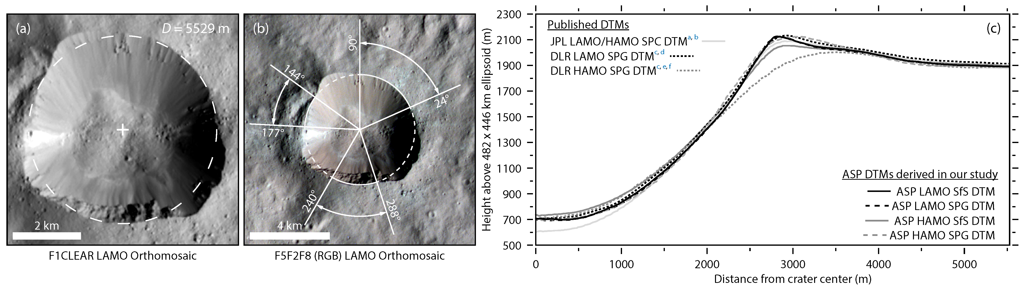
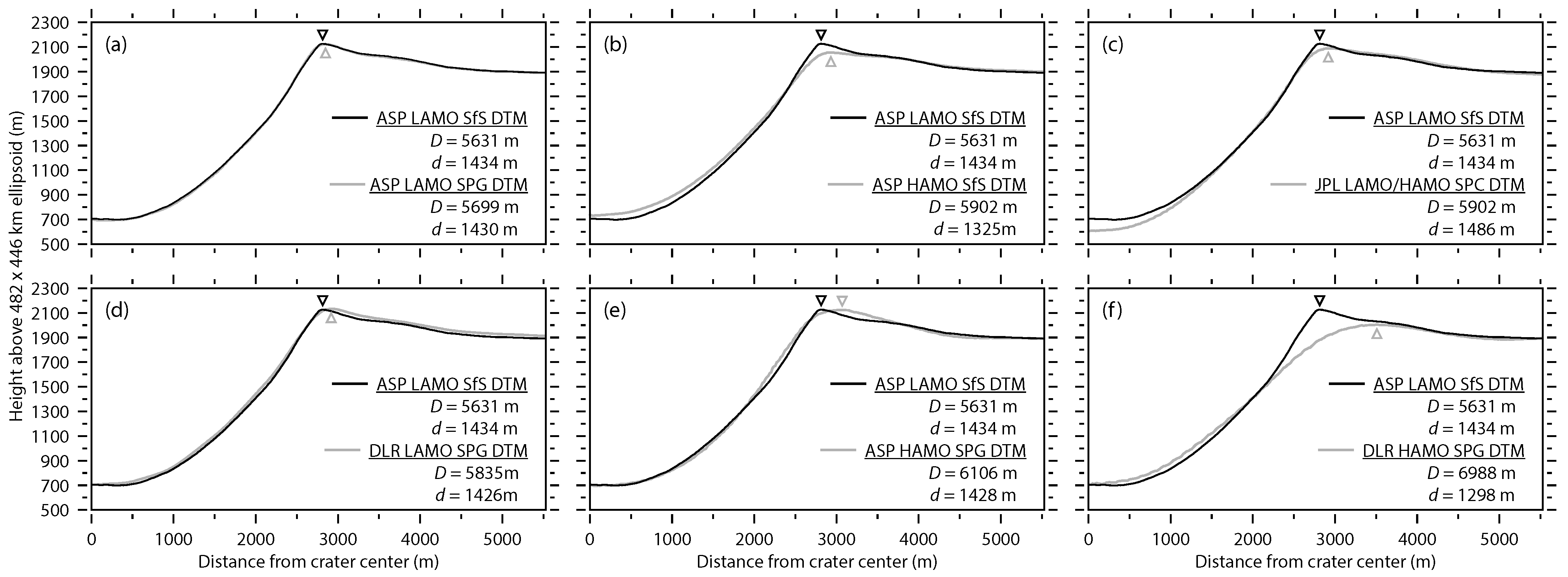
In the following section, we examine the different spatial resolutions of the seven DTMs by focusing on two fresh, texture-rich regions.

5.4.1. Fresh Crater

First, we consider the largest fresh crater (simply called the fresh crater from now on) within our study area, located at 14.281°N_$\phi$ / 233.489°E (12.295°N_$\psi$), which is southwest of the primary ejecta blanket of the young Occator crater, making it younger than Occator. As background information, the formation age of the Occator crater has been estimated to be between 2 and 22 million years (Ma) ago, depending on different chronology and production functions [105]. The fresh crater has a primary (inner) diameter of 5.63 km, and according to our highest resolution CSL/CXL ASP SfS DTM, it has a d/D ratio of 0.255. Such high d/D ratios are typically found in very young craters that have experienced little or no subsequent modification. The fresh crater features a scalloped rim crest, fresh outcrops within its walls, and boulders on its primary ejecta blanket. It also stands out spectroscopically from the surrounding terrain (see Figure 10). Both quantitative and qualitative evidence strongly suggest that this crater is very young, making it ideal for assessing the texture richness of the various DTMs.

Figure 10 presents the fresh crater for each DTM as a semi-transparent, color-coded DTM overlaid on the corresponding hillshade model, the pure hillshade model, an ellipsoid-corrected, photometrically calibrated FC2 clear F1 mosaic, a photometrically corrected FC2 clear F1 mosaic based on the corresponding DTM, and an RGB mosaic (also photometrically corrected using the respective DTM) composed of the F5IR, F2GREEN, and F8BLUE channels. The figure is organized so that the spatial resolution of the DTMs increases from the bottom to the top.

Examining the hillshade models from the bottom to the top, we observe that the lowest spatial resolution was achieved by the DLR HAMO SPG DTM [55,56], while the highest resolution was attained by the CSL/CXL ASP SfS DTM. Both the DLR HAMO [55] and LAMO SPG [104] DTMs, as well as our CSH/CXJ and CSL/CXL SPG DTMs, exhibited artifacts in the eastern crater wall area. This part of the fresh crater lies in shadow in most overlapping HAMO and LAMO image data. The JPL HAMO/LAMO SPC DTM [58,59] and our CSH/CXJ and CSL/CXL ASP SfS DTMs were able to correct these artifacts, as SfS DTM calculations can achieve high-resolution, artifact-free results even with lower resolution multi-temporal coverage. These and other artifacts become more pronounced in the photometrically corrected clear filter and RGB mosaics. It is noteworthy that only the SfS-based DTMs provide sufficient spatial resolution to accurately photometrically correct data from both the HAMO and LAMO.

Looking at the individual panels from left to right in Figure 10, we can see that the spatial resolution of the SPG DTMs was significantly lower than that of the image data used for DTM generation. In contrast, the SfS DTMs allowed for the reconstruction of the topography at a resolution close to that of the image data used for their generation. To highlight this, we focus on the top row of Figure 10, which shows the highest resolution CSL/CXL ASP SfS DTM, with a GSD of 17 m and an effective spatial resolution of ~34 m/px. The corresponding hillshade model reflects all the fine textures in the decameter range that are visible in the original image data (we encourage the reader to zoom into the digital version of the figure or to directly compare the respective DTMs and hillshade models with the F1CLEAR orthomosaics attached to this study). Due to the absence of artifacts and the high resolution, fine spectral differences can now be highlighted, such as the rays radiating from the fresh crater (bright in the photometrically corrected FC2 F1CLEAR mosaic and bright turquoise in the photometrically corrected RGB mosaic). The areas that appear black in the photometrically corrected RGB mosaics are shadowed regions that have been assigned a NODATA value.

Next, we present a more quantitative comparison of the DTMs using topographic profiles. Figure 11 again displays the fresh crater. In the left panel, a photometrically corrected CSL/CXL orthomosaic projected onto the ellipsoid is shown. The dashed line clearly indicates what we previously referred to as the “inner diameter”. After several manual adjustments, the ellipse, and thus the crater center, were positioned to reflect the innermost crater rim crest, avoiding any influence from the scalloped rim crest. This allowed us to derive a sharper rim crest from the topographic profiles. Starting from the crater center, we generated topographic profiles at 3° intervals between azimuths of 24–90°, 144–177°, and 240–288° (see the middle panel in Figure 11). The average profile, derived from 52 individual profiles extracted from each of the seven DTMs, is shown in the right plot of Figure 11.

With the exception of the lowest resolution DTM (the DLR HAMO SPG DTM [55,56]) and the JPL HAMO/LAMO SPC DTM [58,59], the remaining average profiles were consistent, with deviations of approximately ±50 m. As expected, the DLR HAMO SPG DTM [55,56] represented the fresh crater rim as overly flattened. The JPL HAMO/LAMO SPC DTM [58,59] also flattened the crater rim somewhat, but it was approximately 100 m deeper than the other six DTMs at the crater center. The JPL HAMO/LAMO SPC DTM departed visibly from the other DTMs in terms of the crater depth, but the discrepancy was only 3.6%, suggesting that the depths of well-resolved craters were not substantially over- or underestimated in this dataset.

Since many of the profiles in Figure 11 overlap significantly, we reanalyzed them individually in greater detail. In Figure 12, the six profiles are plotted separately, with the highest resolution DTM (CSL/CXJ ASP SfS), which also exhibits the largest d/D ratio, used as the reference (black profiles in the six panels of Figure 12). In Subfigure (a), it is evident that the CSL/CXL (LAMO) SPG and SfS DTMs are practically identical at the given scale. The topographic average profile that most closely matches the one derived from the CSL/CXL ASP SfS DTM is the DLR LAMO SPG DTM. The other five DTMs display a slightly flatter profile, characterized by less steep crater walls and a more subdued crater rim, which is attributed to their lower spatial resolution.

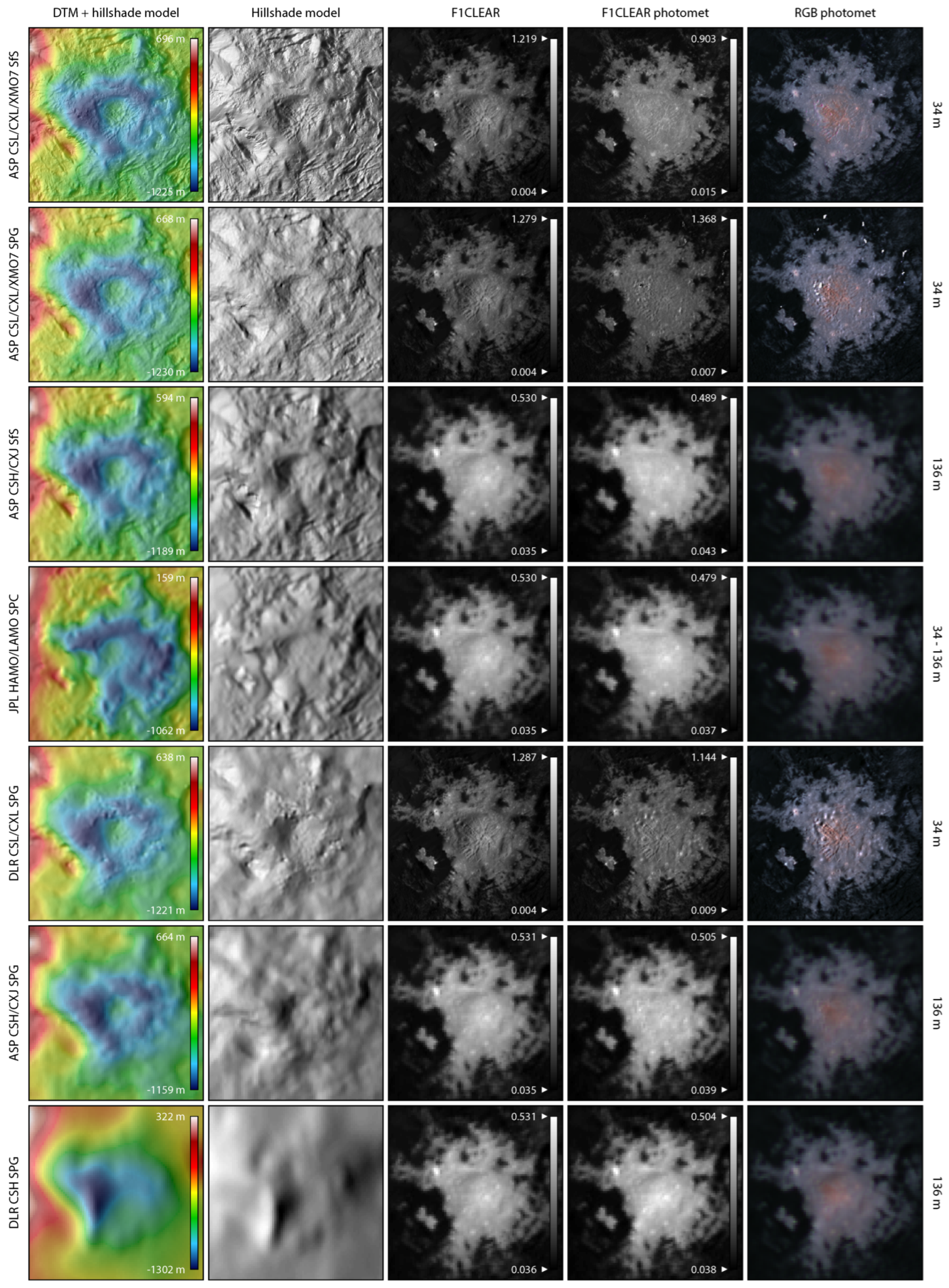
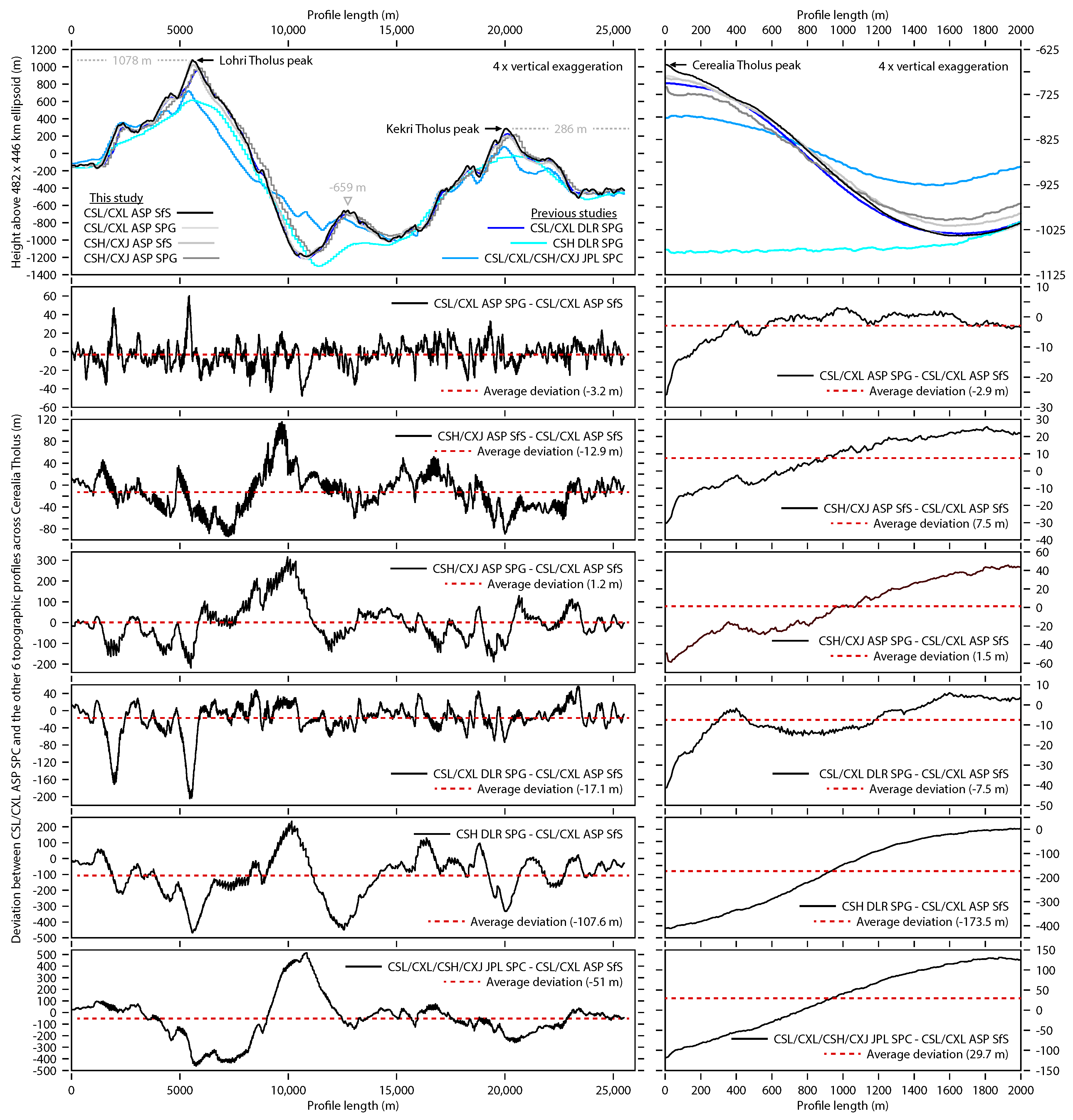
5.4.2. Cerealia Tholus

To evaluate the effectiveness of various approaches for topographic reconstruction, we examined Cerealia Tholus and the bright deposits of Cerealia Facula that cover it. These deposits pose unique challenges for SPG, SfS, and SPC calculations due to their high albedo. As such, the Cerealia Facula serves as a suitable test case for assessing whether our chosen SfS algorithm parameters yield robust and artifact-free results under strong albedo contrasts.

As was performed with the fresh crater in the previous section, Section 5.4.1, we present the results of our four new ASP-derived DTMs alongside the three previously published DTMs. In Figure 13, the seven DTMs are shown as semi-transparent, color-coded DTMs overlaid on the corresponding hillshade model. Additional visualizations include hillshade models alone, two photometrically corrected F1CLEAR orthomosaics based on both a 482 × 446 km ellipsoid and the actual DTM, and an RGB orthomosaic derived from F5IR, F2GREEN, and F8BLUE data, corrected photometrically using the corresponding DTM. This figure was arranged to increase the spatial resolution from the bottom to the top, as can be observed in the leftmost columns displaying the color-coded DTM and hillshade models.

Beginning with the HAMO-based SPG DTM from the DLR, we noted a slightly lower spatial resolution compared to our CSH/CXJ-based ASP SPG DTM. The tholus is morphologically unresolved in the HAMO-based SPG DTM from the DLR but appears as a circular elevation or dome within a depression in the CSH/CXJ-based ASP SPG DTM. In the LAMO-based SPG DTM from the DLR, the tholus appears more detailed, identifiable as a volcanic dome despite minor artifacts. However, fine structures detectable at an LAMO resolution, such as the circular tectonic faults surrounding the Cerealia Tholus recognizable in panel (c) of Figure 14, are absent.

Next, we examined the HAMO/LAMO SPC DTM from the JPL [58,59], where the tholus is distinguishable but notably flatter than in DTMs of a comparable resolution. Our CSH/CXJ-based SfS DTM, despite a slightly lower GSD of 136 m compared to the JPL’s 100 m HAMO/LAMO SPC DTM [58,59], appears to better capture fine structures and accurately reconstruct the Cerealia Facula’s topography.

Figure 14. Overview of the location of the topographic profile across the Cerealia Tholus. We created three different maps, each with their advantages and disadvantages, in order to show which specific surface features are covered by our topographic profile. Our 25,498 m long profile goes from west to east while crossing the highest elevations (the Lohri, Cerealia, and Kekri Tholus) within Occator. (a) Semi-transparent, color-coded CSL/CXL/XMO7 ASP SfS DTM overlaid on the corresponding hillshade model. Topography contour lines are plotted in 100 m intervals. (b) CSL/CXL RGB color composite of Cerealia Facula. (c) Generated slope map overlaid on a curvature map. This combined map highlights aspects of the surface’s shape or features, such as the circular and other rather subparallel fault systems as well as numerous little mounds, at a detailed level.

Figure 14. Overview of the location of the topographic profile across the Cerealia Tholus. We created three different maps, each with their advantages and disadvantages, in order to show which specific surface features are covered by our topographic profile. Our 25,498 m long profile goes from west to east while crossing the highest elevations (the Lohri, Cerealia, and Kekri Tholus) within Occator. (a) Semi-transparent, color-coded CSL/CXL/XMO7 ASP SfS DTM overlaid on the corresponding hillshade model. Topography contour lines are plotted in 100 m intervals. (b) CSL/CXL RGB color composite of Cerealia Facula. (c) Generated slope map overlaid on a curvature map. This combined map highlights aspects of the surface’s shape or features, such as the circular and other rather subparallel fault systems as well as numerous little mounds, at a detailed level.

Lastly, the LAMO-based ASP SPG and SfS DTMs are almost indistinguishable at the scale of Figure 13, but closer inspection reveals that our highest resolution CSL/CXL/XMO7-based ASP SfS DTM resolved all the fine structures visible in the LAMO image data. A comparison of the SPG and SfS topographic profiles further indicates that the high albedo contrast between the Cerealia Facula and the surrounding dark deposits did not produce calculation errors or artifacts.

After conducting a qualitative comparison of the DTMs in the Cerealia Facula area, we then examined absolute elevations through various topographic profiles. To achieve this, we created two profiles. First, we analyzed how well each DTM resolved the highest and lowest areas. The selected topographic profile includes the three peaks of the Lohri, Cerealia, and Kekri Tholus, as well as the lowest area within the central pit. The Lohri and Kekri Tholus constitute two peaks that are remnants of the original central peak. The profile’s path is shown in Figure 14.

In Figure 14, we present three distinct representations of the surface, each with advantages and limitations: In Panel (a), the semi-transparent, color-coded CSL/CXL/XMO7 ASP SfS DTM highlights the topographic features covered by the profile. Panel (b) shows the photometrically corrected CSL/CXL RGB orthomosaic, indicating the albedo variations along the topographic profile. Panel (c) displays a semi-transparent, color-coded slope map derived from the CSL/CXL/XMO7 ASP SfS DTM overlaid on a curvature map. This overlay emphasizes fine surface structures that are not easily visible in panels (a) and (b). The profile and the extracted elevation values from the seven DTMs are presented in Figure 15, which we will discuss in detail below.

In Figure 15, the two columns allow for separate analysis, each containing seven individual plots. In the top plot of the left column, we show the elevation values of the topographic profile from Figure 14 for the seven DTMs. The ASP 2.7 DTMs derived for this study are represented in shades of black to gray, and the previously published DTMs from the DLR [55,56,104] and JPL [58,59] are shown in shades of blue. For the lower panels, we used our highest resolution CSL/CXL/XMO7 ASP SfS DTM as a reference and plotted the deviations of the remaining six DTMs. The average deviations across the profile are also indicated with red dashed lines. The top panel provides a direct comparison, while the lower panels detail specific deviations.

Several noteworthy aspects emerge from the left column. For example, the DLR HAMO-based SPG DTM [55,56] (light blue) at a GSD of 137 m resolved the tholi too flatly compared to the other six DTMs. Our CSH/CXJ-based ASP SPG DTM (dark gray), with a nearly identical GSD of 136 m, already resolves these structures more effectively. The JPL HAMO/LAMO-based SPC DTM [58,59] similarly rendered the tholi and central depression as flatter compared to the five DTMs of an equal or higher resolution. In contrast, the DLR LAMO-based SPG DTM [104] and our CSL/CXL ASP SPG and CSL/CXL/XMO7 ASP SfS DTMs showed only minor differences at the profile scale, with deviations of only a couple 10s of meters. The tholi were most finely resolved in our CSL/CXL/XMO7 ASP SfS DTM.

We now turn to the plots on the right side of Figure 15. Starting from the highest point on the Cerealia Tholus in our CSL/CXL/XMO7 ASP DTM, we created 36 profiles at 10-degree intervals. From these profiles, we calculated an average profile for each DTM and plotted these averages in the upper right panel of Figure 15. Here, the previously noted differences between the DTMs are again evident. While the DLR HAMO-based SPG DTM [55,56] and the JPL HAMO/LAMO-based SPC DTM [58,59] rendered the tholi and central depression too flat, these features appeared significantly more detailed in the remaining five DTMs. The difference between the average lowest point in the central depression and the peak of the Cerealia Tholus shows that our CSL/CXL/XMO7 ASP SfS DTM had the highest peak at 379.4 m. The relative heights of the Cerealia Facula for the other five DTMs were as follows: the CSL/CXL ASP SfS DTM: 355.1 m; LAMO-based DLR SPG DTM [104]: 333.4 m; CSH/CXJ ASP SfS DTM: 327.1 m; CSH/CXJ ASP SPG DTM: 295.0 m; and HAMO/LAMO-based JPL SPC DTM [58,59]: 154.5 m. In the DLR HAMO-based SPG DTM, the tholus was not recognizable in the average profile due to the low spatial resolution. However, since the Cerealia Tholus displays a certain asymmetry, we also provide the maximum height from the peak to the deepest point of the central depression to the west for completeness: the CSL/CXL/XMO7 ASP SfS DTM: 531.5 m; CSL/CXL ASP SPG DTM: 542.2 m; LAMO-based DLR SPG DTM [104]: 521.0 m; CSH/CXJ ASP SfS DTM: 501.0 m; CSH/CXJ ASP SPG DTM: 450.2 m; HAMO/LAMO-based JPL SPC DTM [58,59]: 139.5 m; and HAMO-based DLR SPG DTM [56,107]: 243.0 m.

6. Discussion

Naturally, it is not feasible to discuss all aspects of this study in detail without exceeding the scope of this chapter. Therefore, we will focus our discussion on a few aspects that appear most relevant to our analysis.

6.1. Representational Quality and Generalizability of Our Two Test Sites

The DTMs created in this study cover the entire Occator crater and part of its proximal ejecta blanket. Due to its young age and limited degradation [105], the area exhibits many fine textures and features, including small, fresh impact craters; subparallel and circular fault systems; the various flow fronts of ejected cryolava; mounds of different sizes; steep crater walls with freshly exposed, overhanging outcrops; and, notably, the Cerealia Tholus, Cerealia Facula, and Vinalia Faculae. However, we chose to focus our comparison on just two of these structures (the largest fresh crater in our study area, and the Cerealia Facula/Tholus) to assess the seven DTMs.

This raises the question, are the comparisons of the seven DTMs based on these two sample locations representative and generalizable to the rest of the DTM? The answer is both yes and no, depending on the perspective. In Figure 10, Figure 11 and Figure 12, we illustrate the differences between the seven DTMs in terms of the absolute elevation and spatial resolution, using a medium-sized (5.63 km across), simple, fresh crater as an example. Careful data selection ensured that a potential underestimation of the crater floor elevation, as may occur in SfS and SPC DTMs when long shadows are cast within the crater, was avoided. We did not find evidence of a general underestimation of the crater floor depth or a corresponding low depth-to-diameter ratio in our SfS DTM. On the contrary, our highest resolution CSL/CXL/XMO7 ASP SfS DTM achieved the highest depth-to-diameter ratio (0.255) among all the DTMs. However, this finding is not directly transferable to all other craters. Our example crater is statistically unrepresentative, and future comparative studies would benefit from including additional craters. Moreover, in mid-latitude craters, parts of the crater floors may fall into shadow in overlapping images, likely causing an underestimation of the depth in SfS and SPC DTMs, with this effect increasing as the crater diameter decreases. Nevertheless, the fresh crater serves as a representative case to demonstrate the influence of the DTM’s spatial resolution on the photometric correction of fresh textures and the importance of a high-resolution DTM in achieving artifact-free photometric correction (see Figure 12).

Our second comparison location is inherently non-generalizable, as the bright deposits are unique on Ceres in their extent and contrast with the surrounding terrain. However, this challenging SfS and SPC case allowed us to demonstrate that, even with high albedo contrasts, the SfS calculations with the parameters chosen for the ASP 2.7 achieve robust and largely artifact-free results with multi-temporal coverage. The region around Vinalia Faculae could have served as another comparison area, though it was not explicitly examined here. In our comparison of the two SfS DTMs (CSH/CXJ-based and CSL/CXL/XMO7-based) with the HAMO/LAMO-based SPC DTM, we noted that in the latter, the bright deposits were modeled as a westward-shifted elevation (for reference, the average subsolar ground azimuth is ~102°). As there are numerous other areas within our DTMs where the quality differences of the individual DTMs, as well as the distinctions between SPG, SfS, and SPC approaches, can be assessed, we encourage interested users of our DTMs to conduct their own comparisons.

6.2. Errors Between Different DTMs

Errors in DTM generation can generally be divided into two categories. In SPG DTM generation, triangulation errors exceeding acceptable thresholds are excluded. This ensures that points with errors greater than 68 m (CSH/CXJ) or 17 m (CSL/CXL)—approximately half the pixel size of the image data used—are not included in the raster DTM. Further outliers and artifacts are filtered using kernel-based methods (see Section 4.5.3). While most 3D points have lower triangulation errors, we conservatively estimated maximum height errors of 68 m and 17 m, based on the resolution of the image data used.

Interpolation to the final raster DTM was conducted at a GSD roughly corresponding to the actual spatial resolution. It is important to note that, even when the 3D point cloud density matches the pixel size of the image data, the spatial resolution of an interpolated DTM is at least 3–5 times lower [72]. For example, a hillshade model generated from the HAMO-based SPG DTM [55,56] created by the DLR was visually closest to a hillshade model generated from our higher resolution CSH/CXJ-based SPC DTM (68 m), though downscaled to 680 m, over the Occator crater region. A similar 6:1 ratio between the actual spatial resolution and the GSD used was observed for the LAMO-based SPG DTM [104] created by the DLR. Comparisons between our SfS and SPG DTMs indicate an effective spatial resolution of about 4–5 pixels for our SPG DTMs. However, both our DTMs and those created by the DLR for the HAMO [55,56] and LAMO [104] use a GSD that matches the resolution of the original image data.

Another approach to assess the DTM accuracy is through the Root Mean Square Error (RMSE) or Mean Absolute Error (MAE) based on deviations from reference points or ground control points (GCPs) with high elevation accuracy. Since no high-accuracy GCPs, such as those generated by a laser altimeter, exist for Ceres, we omitted this method.

As described in Section 5, due to differences in the image data and generation methods (SPG, SfS, and SPC), we opted for an inter-model comparison. We calculated average and standard deviations for differences between the SPG and SfS DTMs and among SPG DTMs of different resolutions (Table 4 and Table 5). Two key insights emerged: (1) Our SPG and SfS DTMs differed by 1.89 m (CSH/CXJ) and 3.64 m (CSL/CXL), with standard deviations of 30.5 m and 10.5 m, respectively, suggesting robustness in the SfS DTMs optimized from the SPG inputs. (2) Our CSL/CXL SPG DTM differs, on average, by only 0.65 m from the lower resolution CSH/CXL SPG DTM, with a standard deviation of 31.7 m. For comparison, the LAMO-based SPG DTM [104] from the DLR shows an average difference of 3.65 m and a standard deviation of 78.8 m from the HAMO-based SPG DTM [55,56]. Although these values offer insights into the average deviations, they do not reveal the spatial variability. To address this, we subdivided deviations by the latitude and longitude, allowing us to observe long-wavelength deviations (Figure 8). Notably, there is a southwest-to-northeast trend between the HAMO-based [55,56] and LAMO-based [104] SPG DTMs (both created by the DLR), with the LAMO-based DTM [104] being up to 25 m higher in the southwestern area (area 3) and up to 45 m lower in the northeast, relative to the HAMO-based DTM [55,56] (see Figure 8). These deviations exceed the stated height accuracies of 10 m (HAMO) and 1.5 m (LAMO).

For further comparison, we used the HAMO-based SPG DTM [55,56] created by the DLR as a reference, examining its deviations relative to our CSH/CXJ SPG and SfS DTMs and the HAMO/LAMO SPC DTM from the JPL [55,56,104]. Average deviations and standard deviations are given in Table 5. Figure 9 shows, for instance, that the HAMO/LAMO-based SPC DTM from the JPL [58,59] varies on average by −30.0 m and −17.4 m for areas 1 and 4, respectively. Since this DTM also has a stated average height accuracy of 10 m, these deviations exceed the specified error range.

In conclusion, we observed that the SPG DTMs from the DLR and the SPC DTM from the JPL show average deviations in our comparison regions that sometimes exceed their stated height accuracies. They suggest that there may be unaccounted-for sources of error or systematic biases in one or more of the DTMs. Possible causes include vertical offsets, variations in methods, and different image data used in DTM generation. To clarify, we are not questioning the quality of the published DTMs; rather, we noted these discrepancies and therefore did not use any specific DTM as a reference for aligning our DTMs.

6.3. Influence of Photometric Models on SfS and SPC

In SfS and SPC, the photometric model plays a crucial role in interpreting how light reflects off the surface and directly affects the accuracy of DTM generation. SPC relies on brightness gradients in images to infer slopes. The photometric model provides a mathematical framework for relating brightness values to slopes by accounting for the angle of incidence, reflection, and scattering behavior of the surface material. If this model is incorrect or overly simplistic, the derived slopes will be inaccurate, affecting the resulting terrain heights and shapes.

We used the modified Hapke model implemented in the ASP, with corresponding values from [99] (see Section 4.3). This approach differs from the photometric model used in creating the HAMO/LAMO-based SPC DTM from the JPL [27,59], which combines Lambert and Lommel–Seeliger reflectance functions. Another distinction between our DTM and the HAMO/LAMO-based SPC DTM from the JPL [27,59] is that we first generated a lower resolution SPG DTM, which served as the foundation for SfS DTM generation. By utilizing the --smoothness-weight and --initial-dem-constraint-weight parameters integrated into the SfS function of the ASP, we were able to further constrain deviations of the SfS DTM from the lower resolution but generally more robust SPG DTM, helping to minimize or even prevent artifacts and discrepancies.

Due to differences in the algorithms used to calculate slopes and, ultimately, to derive the SfS DTM, it is expected that the resulting SfS DTMs may show slight variations and height errors compared to one another.

6.4. Influence of Faculae on SfS and SPC DTMs (ASP 2.7 and JPL)

While we have previously examined the impact of strong albedo contrasts on SfS DTM generation with Cerealia Facula (Figure 13 and Figure 14), here we consider another practical example. Unlike Cerealia Facula, which primarily consists of contiguous bright deposits with sharp boundaries against surrounding darker material, Vinalia Faculae comprise more diffuse, gradually thinning bright deposits. To investigate this, we analyzed a profile extending from WSW to ENE across the two largest regions of the Vinalia Faculae (dashed line in panels (c) and (d) of Figure 16). For comparison, we used the slightly lower resolution but robust CSL/CXL ASP SPG DTM, which is unaffected by the faculae (dark gray line in panel (a) of Figure 16). We then extracted elevation values from the two highest resolution SfS and SPC DTMs: the CSL/CXL ASP SfS DTM and the JPL HAMO/LAMO-based SPC DTM (dark gray and blue lines in panel (a) of Figure 16). Additionally, to better visualize any relationship between the albedo and topographic profiles, we plotted the albedo from the photometrically corrected F1CLEAR CSL/CXL orthomosaic as a light gray line in panel (a) of Figure 16.

The rugged terrain associated with cryolava, as shown in the CSL/CXL ASP SfS DTM in panel (c) of Figure 16, also appears as short-wavelength fluctuations in the topographic profiles. Of particular interest, however, are the long-wavelength fluctuations in the topographic profiles, which may indicate an influence of the albedo. In panel (a) of Figure 16, we observe that our CSL/CXL ASP SfS DTM correlates well with the CSL/CXL ASP SPG DTM, showing only minor deviations. Vinalia Faculae seem to have a larger effect on the calculation of the JPL HAMO/LAMO-based SPC DTM. To facilitate comparison, we used the CSL/CXL ASP SPG DTM as a reference, as it should be unaffected by strong albedo contrasts due to its feature-based correlation and triangulation. In panel (c) of Figure 16, we compare the derived CSL/CXL ASP SfS DTM with the JPL HAMO/LAMO-based SPC DTM. The dashed lines indicate the average deviations over the entire profile: +3.3 m for the CSL/CXL ASP SfS DTM and −33.7 m for the JPL HAMO/LAMO-based SPC DTM. Between our CSL/CXL ASP SPG and SfS DTMs, we observe a weak, long-wavelength deviation of approximately ±10 m, which could be related to the faculae. More notably, the JPL HAMO/LAMO-based SPC DTM shows a strong, long-wavelength deviation of up to ±140 m relative to our CSL/CXL ASP SPG DTM. Given that the average solar azimuth of 102° indicates sunlight from the east, it seems plausible that the SPC algorithms may misinterpret the bright deposits as a slope inclined towards the east.

To reduce the influence of albedo differences on slope and elevation calculations in the SfS DTM, adjustments to the --smoothness-weight and --initial-dem-constraint-weight options in the ASP 2.7 may be effective. Alternatively, the SfS DTM could be co-registered to the more robust SPG DTM. The ASP’s pc_align function employs an Iterative Closest Point (ICP) co-registration approach to align a higher resolution DTM with a lower resolution DTM through rotation, translation, and scaling adjustments.

7. Conclusions

Our study presents significant advancements in the digital terrain modeling of the Occator crater on Ceres, specifically targeting the bright deposits of the Cerealia Facula and Vinalia Faculae. Using data collected by NASA’s Dawn mission, we developed improved SPG and SfS DTMs of the Occator crater at various resolutions. These models aim to support future landing site assessments and sample return mission planning by providing a detailed topographical understanding of a complex geomorphological region.

We believe that these new data products open a number of opportunities for future research, including quantitative geomorphologic and geologic as well as structural and tectonic studies, which ultimately provide better insights into cratering processes and the planet’s crater chronology, erosional processes, weathering, and also endogenic processes including structural developments and the development of cryovolcanism. These data products would allow for more detailed compositional analyses based on albedo characteristics and provide a basis for future landing site studies in which impact crater sizes, depths, slopes, and rock size distributions will be fundamental parameters required for assessment. Lastly, these data products could form a high-fidelity basis for exobiology studies, studies on preserving biosignatures, and habitability modeling.

A central challenge we tackled was the significant albedo (brightness) variation within the Occator crater, particularly around the high-albedo regions of the Cerealia and Vinalia Faculae. These areas create unique obstacles for topographic modeling, as traditional photometric methods can struggle with such contrasts. To overcome these challenges, we developed and fine-tuned workflows involving high-resolution SPG and multi-view SfS techniques, leveraging tools like the USGS ISIS 3 and the ASP 2.7. Through these methods, we achieved finer resolution DTMs with grid spacings down to 17 m and resolutions at the image scale, which is an improvement over previously published and archived DTMs.

All the DTMs and their corresponding orthomosaics produced in this study are publicly available. Detailed information about these data products can be found in the accompanying documentation.

Our main conclusions can be summarized as follows:

• Improved Co-Registration and Data Alignment: Our manual, iterative co-registration multi-mission process aligns Dawn’s imaging data accurately, minimizing offsets that could hinder the model’s precision. While we observed offsets of up to 2–3 pixels between the DLR and JPL data products in the Occator crater region, our HAMO- and LAMO-based DTMs and orthomosaics are precisely aligned, with an average offset of approximately 0.5 pixels. This step is critical for SPG, SfS, and SPC approaches, ensuring the alignment of multi-temporal and multi-angle datasets. The new DTMs also improve the orthorectification quality and thus further minimize the offsets between overlapping images, specifically those acquired at high emission angles.
• Resolution and Grid Spacing: Our new DTMs offer significantly enhanced grid spacing and resolution, down to 17 m and 34 m/px compared to the LAMO-based SPG DTM from the DLR (32 m) and the HAMO/LAMO-based SPC DTM from the JPL (100 m). More important than the GSD, however, is the effective resolution. Compared to our CSL/CXL ASP SPC DTM, which has a GSD and resolution of 17 m and 34 m/px, the LAMO-based SPG DTM from the DLR, which was processed to an almost identical GSD of 32 m, appears to be oversampled by a factor of about 4–5. As we have shown at our two example sites, the finer resolution of our DTMs allows for a more detailed view of geomorphologic features, enabling more precise analyses of terrain features (e.g., through surface slope and roughness analyses) for landing site selection.
• Enhanced Detail and Reduction in Artefacts: Using a combination of SPG and SfS, the new DTMs provide a more detailed surface reconstruction and reduce the artifacts that appear in prior models. This combination approach allows the new DTMs to capture fine topographic details in smooth regions and high-contrast zones, which were previously difficult to model accurately. The resulting DTMs feature clearer delineations of Occator’s cryovolcanic structures, such as the fractured dome of the Cerealia Tholus and the thinner dispersed Vinalia Faculae deposits.
• Topographic Accuracy in High-Albedo Regions: Previous DTMs struggled with accuracy in high-albedo areas like the Cerealia Facula and Vinalia Faculae due to their reflective properties, which created challenges in traditional photometric topography reconstruction. The new DTMs developed in this study integrate custom photometric corrections that mitigate the effects of a high brightness contrast, capturing these regions with improved clarity and topographic fidelity. Despite the exceptionally high albedo variations observed in the study area, the DTMs show a consistently high quality and suggest that multi-view shape-from-shading with albedo modeling has the potential to produce convincing results for other planetary bodies as well.
• Impact on Photometric Correction: The SfS DTMs created in this study have a significantly positive impact on the quality of the photometric correction. On the one hand, the improved co-registration combined with more accurate orthorectification already reduces the offsets at topographically exposed areas (e.g., sharply defined crater rims). These offsets, when using lower resolution DTMs for orthorectification, previously resulted in false color seamlines in RGB composites. Photometric correction is always only as accurate as the underlying DTM. Since our SfS DTMs match the resolution of the image data, they meet the requirements for achieving photometric correction with minimal artifacts.
• Replicability: Both DLR and JPL use proprietary in-house software for data processing and DTM generation, which can make it challenging for external researchers to trace individual processing steps and reproduce their results. In contrast, our work relies exclusively on free and open-source software commonly used in the planetary science community, specifically the ISIS 3 and the ASP 2.7. This approach ensures the accessible reproducibility of our data products, although it is computation- and time-intensive and requires suitable resources. We have provided a detailed description of our methodology for using these tools to aid future researchers who may apply them in other contexts.

8. Foresight

Our results do not represent the highest achievable GSD and resolution for DTMs in the Occator crater region. For the DTMs provided in this study, we used only FC data from the F1CLEAR filter, although we have begun experimenting with incorporating narrow-band filter data (F2GREEN, F5IR, F7RED) for DTM generation. These preliminary results suggest that the future inclusion of narrow-band filter data may enhance the 3D point density in SPG DTM generation.

Our work primarily used data acquired during the HAMO and LAMO phases. Additionally, we selectively included data from the highly elliptical XMO7 orbit, with GSDs between 38 and 17 m, in CSL/CXL ASP SfS DTM generation to increase the multi-temporal coverage with low emission angle image frames. During XMO7, over 1000 FC1 and FC2 datasets with GSDs as high as 2.7 m were acquired of the Occator crater’s interior. Incorporating these highest resolution data in future efforts could enable the generation of an even higher resolution, continuous DTM—particularly for areas of interest around the faculae for potential landing site missions. However, because the XMO7 data vary significantly in terms of the resolution due to the orbit’s strong ellipticity, future DTMs must assess the multi-temporal coverage relative to the spatial resolution. This is crucial, as robust SfS DTM calculations of the high-contrast faculae require repeated coverage under varying solar incidence and directional angles. It is also worth exploring the integration of super-resolution methods into the pre-processing pipeline. However, given the maximum GSD of 2.7 m for some individual FC1 and FC2 F1CLEAR XMO7 images, achieving comprehensive DTM coverage with GSDs greater than or equal to 2.7 m for the entire interior of the Occator crater remains unlikely.

References

1. Anderson, J.D.; Schubert, G.; Jacobson, R.A.; Lau, E.L.; Moore, W.B.; Sjogren, W.L. Europa’s Differentiated Internal Structure: Inferences from Four Galileo Encounters. Science 1998, 281, 2019–2022. [Google Scholar] [CrossRef] [PubMed]
2. Carr, M.H.; Belton, M.J.S.; Chapman, C.R.; Davies, M.E.; Geissler, P.; Greenberg, R.; McEwen, A.S.; Tufts, B.R.; Greeley, R.; Sullivan, R.; et al. Evidence for a subsurface ocean on Europa. Nature 1998, 391, 363–365. [Google Scholar] [CrossRef] [PubMed]
3. Khurana, K.K.; Kivelson, M.G.; Stevenson, D.J.; Schubert, G.; Russell, C.T.; Walker, R.J.; Polanskey, C. Induced magnetic fields as evidence for subsurface oceans in Europa and Callisto. Nature 1998, 395, 777–780. [Google Scholar] [CrossRef] [PubMed]
4. Kivelson, M.G.; Khurana, K.K.; Stevenson, D.J.; Benett, L.; Joy, S.; Russell, C.T.; Walker, R.J.; Zimmer, C.; Polanskey, C. Europa and Callisto: Induced or intrinsic fields in a periodically varying plasma environment. J. Geophys. Res. 1999, 104, 4609–4625. [Google Scholar]
5. Zimmer, C.; Khurana, K.K.; Kivelson, M.G. Subsurface Oceans on Europa and Callisto: Constraints from Galileo Magnetometer Observations. Icarus 2000, 147, 329–347. [Google Scholar] [CrossRef]
6. Khurana, K.K.; Kivelson, M.G.; Hand, K.P.; Russell, C.T. Europa; Space Science Series; University of Arizona Press: Tucson, AZ, USA, 2009; Chapter Electromagnetic Induction from Europa’s Ocean and the Deep Interior; pp. 571–588. [Google Scholar]
7. Schubert, G.; Sohl, F.; Hussmann, H. Europa; Space Science Series; University of Arizona Press: Tucson, AZ, USA, 2009; Chapter Interior of Europa; pp. 353–368. [Google Scholar]
8. Postberg, F.; Kempf, S.; Schmidt, J.; Brilliantov, N.; Beinsen, A.; Abel, B.; Buck, U.; Srama, R. Sodium salts in E-ring ice grains from an ocean below the surface of Enceladus. Nature 2009, 459, 1098–1101. [Google Scholar] [CrossRef]
9. Iess, L.; Stevenson, D.J.; Parisi, M.; Hemingway, D.; Jacobson, R.A.; Lunine, J.I.; Nimmo, F.; Armstrong, J.W.; Asmar, S.W.; Ducci, M.; et al. The Gravity Field and Interior Structure of Enceladus. Science 2014, 34, 78–80. [Google Scholar] [CrossRef]
10. Beuthe, M.; Rivoldini, A.; Trinh, A. Enceladus’s and Dione’s floating ice shells supported by minimum stress isostasy. Geophys. Res. Lett. 2016, 43, 10088–10096. [Google Scholar] [CrossRef]
11. Čadek, O.; Tobie, G.; van Hoolst, T.; Massé, M.; Choblet, G.; Lefèvre, A.; Mitri, G.; Baland, R.M.; Běhounková, M.; Bourgeois, O.; et al. Enceladus’s internal ocean and ice shell constrained from Cassini gravity, shape, and libration data. Geophys. Res. Lett. 2016, 43, 5653–5660. [Google Scholar] [CrossRef]
12. Thomas, P.; Tajeddine, R.; Tiscareno, M.S.; Burns, J.A.; Joseph, J.; Loredo, T.J.; Helfenstein, P.; Porco, C. Enceladus’s measured physical libration requires a global subsurface ocean. Icarus 2016, 264, 37–47. [Google Scholar] [CrossRef]
13. Hemingway, D.; Iess, L.; Tajeddine, R.; Tobie, G. Enceladus and the Icy Moons of Saturn; Arizona of University Press: Tucson, AZ, USA, 2018; Chapter The Interior of Enceladus; pp. 57–77. [Google Scholar] [CrossRef]
14. Lorenz, R.D.; Stiles, B.W.; Kirk, R.L.; Allison, M.D.; Del Marmo, P.P.; Iess, L.; Lunine, J.I.; Ostro, S.J.; Hensley, S. Titan’s Rotation Reveals an Internal Ocean and Changing Zonal Winds. Science 2008, 319, 1649–1651. [Google Scholar] [CrossRef] [PubMed]
15. Iess, L.; Jacobson, R.A.; Ducci, M.; Stevenson, D.J.; Lunine, J.I.; Armstrong, J.W.; Asmar, S.W.; Racioppa, P.; Rappaport, N.J.; Tortora, P. The Tides of Titan. Science 2012, 337, 457–459. [Google Scholar] [CrossRef]
16. Mitri, G.; Meriggiola, R.; Hayes, A.; Lefevre, A.; Tobie, G.; GEnova, A.; Lunine, J.I.; Zebker, H. Shape, topography, gravity anomalies and tidal deformation of Titan. Icarus 2014, 236, 169–177. [Google Scholar] [CrossRef]
17. Saur, J.; Duling, S.; Roth, L.; Jia, X.; Strobel, D.F.; Feldman, P.D.; Christensen, U.R.; Retherford, K.D.; McGrath, M.A.; Musacchio, F.; et al. The search for a subsurface ocean in Ganymede with Hubble Space Telescope observations of its auroral ovals. J. Geophys. Res. Space Phys. 2015, 120, 1715–1737. [Google Scholar] [CrossRef]
18. Hendrix, A.R.; Hurford, T.A.; Barge, L.M.; Bland, M.T.; Bowman, J.S.; Brinckerhoff, W.; Buratti, B.J.; Cable, M.L.; Castillo-Rogez, J.; Collins, G.C.; et al. The NASA Roadmap to Ocean Worlds. Astrobiology 2019, 19, 1–27. [Google Scholar] [CrossRef]
19. Nimmo, F.; Spencer, J.R. Powering Triton’s recent geological activity by obliquity tides: Implications for Pluto geology. Icarus 2015, 246, 2–10. [Google Scholar] [CrossRef]
20. Bierson, C.J.; Nimmo, F.; Stern, S.A. Evidence for a hot start and early ocean formation on Pluto. Nat. Geosci. 2020, 13, 468–472. [Google Scholar] [CrossRef]
21. Denton, C.A.; Johnson, B.C.; Wakita, S.; Freed, A.M.; Melosh, H.J.; Stern, S.A. Pluto’s Antipodal Terrains Imply a Thick Subsurface Ocean and Hydrated Core. Geophys. Res. Lett. 2021, 48, e2020GL091596. [Google Scholar] [CrossRef]
22. Fu, R.R.; Ermakov, A.I.; Marchi, S.; Castillo-Rogez, J.C.; Raymond, C.A.; Hager, B.H.; Zuber, M.T.; King, S.D.; Bland, M.T.; De Sanctis, M.C.; et al. The Interior Structure of Ceres as Revealed by Surface Topography. Earth Planet. Sci. Lett. 2017, 476, 153–164. [Google Scholar] [CrossRef]
23. Russell, C.T.; Raymond, C.A. The Dawn Mission to Vesta and Ceres. Space Sci. Rev. 2011, 163, 3–23. [Google Scholar] [CrossRef]
24. De Sanctis, M.C.; Ammannito, E.; Raponi, A.; Frigeri, A.; Ferrari, M.; Carrozzo, F.G.; Ciarniello, M.; Formisano, M.; Rousseau, B.; Tosi, F.; et al. Fresh emplacement of hydrated sodium chloride on Ceres from ascending salty fluids. Nat. Astron. 2020, 4, 786–793. [Google Scholar] [CrossRef]
25. De Sanctis, M.C.; Mitri, G.; Castillo-Rogez, J.; House, C.H.; Marchi, S.; Raymond, C.A.; Sekine, Y. Relict Ocean Worlds: Ceres. Space Sci. Rev. 2020, 216, 60. [Google Scholar] [CrossRef]
26. Nathues, A.; Schmedemann, N.; Thangjam, G.; Pascker, J.H.; Mengel, K.; Castillo-Rogez, J.C.; Cloutis, E.A.; Hiesinger, H.; Hoffmann, M.; Le Corre, L.; et al. Recent cryovolcanic activity at Occator crater on Ceres. Nat. Astron. 2020, 4, 794–801. [Google Scholar] [CrossRef]
27. Park, R.S.; Konopliv, A.S.; Ermakov, A.I.; CastilloRogez, J.C.; Fu, R.R.; Hughson, K.H.G.; Prettyman, T.H.; Raymond, C.A.; Scully, J.E.C.; Sizemore, H.G.; et al. Evidence of non-uniform crust of Ceres from Dawn’s high-resolution gravity data. Nat. Astron. 2020, 4, 748–755. [Google Scholar] [CrossRef]
28. Raymond, C.A.; Ermakov, A.I.; Castillo-Rogez, J.C.; Marchi, S.; Johnson, B.C.; Hesse, M.A.; Scully, J.E.C.; Buczkowski, D.L.; Sizemore, H.G.; Schenk, P.M.; et al. Impact-driven mobilization of deep crustal brines on dwarf planet Ceres. Nat. Astron. 2020, 4, 741–747. [Google Scholar] [CrossRef]
29. Schenk, P.; Scully, J.; Buczkowski, D.; Sizemore, H.; Schmidt, B.; Pieters, C.; Neesemann, A.; O’Brien, D.; Marchi, S.; Williams, D.; et al. Impact heat driven volatile redistribution at Occator crater on Ceres as a comparative planetary process. Nat. Commun. 2020, 11, 3679. [Google Scholar] [CrossRef]
30. Schmidt, B.E.; Sizemore, H.G.; Hughson, K.H.G.; Duarte, K.D.; Romero, V.N.; Scully, J.E.C.; Schenk, P.M.; Buczkowski, D.L.; Williams, D.A.; Nathues, A.; et al. Post-impact cryo-hydrologic formation of small mounds and hills in Ceres’s Occator crater. Nat. Geosci. 2020, 13, 605–610. [Google Scholar] [CrossRef]
31. Scully, J.E.C.; Schenk, P.M.; Castillo-Rogez, J.C.; Buczkowski, D.L.; Williams, D.A.; Pasckert, J.H.; Duarte, K.D.; Romero, V.N.; Quick, L.C.; Sori, M.M.; et al. The varied sources of faculae-forming brines in Ceres’ Occator crater emplaced via hydrothermal brine effusion. Nat. Commun. 2020, 11, 3680. [Google Scholar] [CrossRef]
32. Castillo-Rogez, J.; Neveu, M.; McSween, H.Y.; Fu, R.R.; Toplis, M.J.; Prettyman, T. Insights into Ceres’s evolution from surface composition. Meteorit. Planet. Sci. 2018, 53, 1820–1843. [Google Scholar] [CrossRef]
33. Park, R.S.; Konopliv, A.S.; Bills, B.G.; Rambaux, N.; Castillo-Rogez, J.C.; Raymond, C.A.; Vaughn, A.T.; Ermakov, A.I.; Zuber, M.T.; Fu, R.R.; et al. A partially differentiated interior for (1) Ceres deduced from its gravity field and shape. Nature 2016, 537, 515–517. [Google Scholar] [CrossRef]
34. Ermakov, A.I.; Fu, R.R.; Castillo-Rogez, J.C.; Raymond, C.A.; Park, R.S.; Preusker, F.; Russell, C.T.; Smith, D.E.; Zuber, M.T. Constraints on Ceres’ Internal Structure and EvolutionFrom Its Shape and Gravity Measuredby the Dawn Spacecraft. J. Geophys. Res. 2017, 122, 2267–2293. [Google Scholar] [CrossRef]
35. Konopliv, A.S.; Park, R.S.; Vaughn, A.T.; Bills, B.G.; Asmar, S.W.; Ermakov, A.I.; Rambaux, N.; Raymond, C.A.; Castillo-Rogez, J.C.; Russell, C.T.; et al. The Ceres gravity field, spin pole, rotation period and orbit from the Dawn radiometric tracking and optical data. Icarus 2018, 299, 411–429. [Google Scholar] [CrossRef]
36. Prettyman, T.H.; Yamashita, N.; Toplis, M.J.; McSween, H.Y.; Schörghofer, N.; Marchi, S.; Feldman, W.C.; Castillo-Rogez, J.; Forni, O.; Lawrence, D.J.; et al. Extensive water ice within Ceres’ aqueously altered regolith: Evidence from nuclear spectroscopy. Science 2017, 355, 55–59. [Google Scholar] [CrossRef] [PubMed]
37. Prettyman, T.H.; Yamashita, N.; Landis, M.E.; Castillo-Rogez, J.C.; Schörghofer, N.; Pieters, C.M.; Sizemore, H.G.; Hiesinger, H.; Marchi, S.; McSween, H.Y.; et al. Replenishment of Near-Surface Water Ice by Impacts Into Ceres’ Volatile-Rich Crust: Observations by Dawn’s Gamma Ray and Neutron Detector. Geophys. Res. Lett. 2021, 48, e2021GL094223. [Google Scholar] [CrossRef]
38. Ruesch, O.; Platz, T.; Schenk, P.; McFadden, L.A.; Castillo-Rogez, J.C.; Quick, L.C.; Byrne, S.; Preusker, F.; O’Brien, D.P.; Schmedemann, N.; et al. Cryovolcanism on Ceres. Science 2016, 353, aaf4286. [Google Scholar] [CrossRef]
39. De Sanctis, M.C.; Raponi, A.; Amannito, A.; Ciarniello, M.; Toplis, M.J.; McSween, H.Y.; Castillo-Rogez, J.C.; Ehlmann, B.L.; Carrozzo, F.G.; Marchi, S.; et al. Bright carbonate deposits as evidence of aqueous alteration on (1) Ceres. Nature 2016, 536, 54–57. [Google Scholar] [CrossRef]
40. Ruesch, O.; Quick, L.C.; Landis, M.E.; Sori, M.M.; Čadek, O.; Brož, P.; Otto, K.A.; Bland, M.T.; Byrne, S.; Castillo-Rogez, J.C.; et al. Bright Carbonate Surfaces on Ceres as Remnants of Salt-Rich Water Fountains. Icarus 2019, 320, 39–48. [Google Scholar] [CrossRef]
41. Scully, J.E.; Baker, S.R.; Castillo-Rogez, J.C.; Buczkowski, D.L. The In Situ Exploration of a Relict Ocean World: An Assessment of Potential Landingand Sampling Sites for a Future Mission to the Surface of Ceres. Planet. Sci. J. 2021, 2, 94. [Google Scholar] [CrossRef]
42. Gassot, O.; Panicucci, P.; Acciarini, G.; Bates, H.; Caballero, M.; Cambianica, P.; Dziewiecki, M.; Dionnet, Z.; Enengl, F.; Gerig, S.B.; et al. Calathus: A sample-return mission to Ceres. Acta Astronaut. 2021, 181, 112–129. [Google Scholar] [CrossRef]
43. Castillo-Rogez, J.; Brophy, J.; Miller, K.; Sori, M.; Scully, J.; Quick, L.; Grimm, R.; Zolensky, M.; Bland, M.; Buczkowski, D.; et al. Concepts for the Future Exploration of Dwarf Planet Ceres’ Habitability. Planet. Sci. J. 2022, 3, 41. [Google Scholar] [CrossRef]
44. National Academies of Sciences, Engineering, and Medicine. Origins, Worlds, and Life. A Decadal Strategy for Planetary Science and Astrobiology 2023–2032; The National Academies Press: Cambridge, MA, USA, 2023. [Google Scholar] [CrossRef]
45. Castillo-Rogez, J. Future exploration of Ceres as an ocean world. Nat. Astron. 2020, 4, 732–734. [Google Scholar] [CrossRef]
46. Kirk, R.; Howington-Kraus, E.; Rosiek, M.; Anderson, J.; Archinal, B.; Becker, K.; Cook, D.; Galuszka, D.; Geissler, P.; Hare, T.; et al. Ultrahigh resolution topographic mapping of Mars with MROHiRISE stereo images: Meter-scale slopes of candidate Phoenixlanding sites. J. Geophys. Res. 2008, 113. [Google Scholar] [CrossRef]
47. Sierks, H.; Keller, H.U.; Jaumann, R.; Michalik, H.; Behnke, T.; Bubenhagen, F.; Büttner, I.; Carsenty, U.; Christensen, U.; Enge, R.; et al. The Dawn Framing Camera. Space Sci. Rev. 2011, 163, 263–327. [Google Scholar] [CrossRef]
48. Beyer, R.A.; Alexandrov, O.; McMichael, S. The Ames Stereo Pipeline: NASA’s Open Source Software for Deriving and Processing Terrain Data. Earth Space Sci. 2018, 5, 537–548. [Google Scholar] [CrossRef]
49. Alexandrov, O.; Beyer, R.A. Multiview Shape-From-Shading for Planetary Images. Earth Space Sci. 2018, 5, 652–666. [Google Scholar] [CrossRef]
50. Thomas, V.C.; Makowski, J.M.; Brown, G.M.; McCarthy, J.F.; Bruno, D.; Cardoso, J.C.; Chiville, W.M.; Meyer, T.F.; Nelson, K.E.; Pavri, B.E.; et al. The Dawn Spacecraft. Space Sci. Rev. 2011, 163, 175–249. [Google Scholar] [CrossRef]
51. De Sanctis, M.; Coradini, A.; Ammannito, E.; Filacchione, G.; Capria, M.; Fonte, S.; Magni, G.; Barbis, A.; Bini, A.; Dami, M.; et al. The VIR Spectrometer. Space Sci. Rev. 2011, 163, 329–369. [Google Scholar] [CrossRef]
52. Prettyman, T.H.; Feldman, W.C.; McSween, H.Y., Jr.; Dingler, R.D.; Enemark, D.C.; Patrick, D.E.; Storms, S.A.; Hendricks, J.S.; Morgenthaler, H.P.; Pitman, K.M.; et al. Dawn’s Gamma Ray and Neutron Detector. Space Sci. Rev. 2011, 163, 371–459. [Google Scholar] [CrossRef]
53. Konopliv, A.; Asmar, S.; Bills, B.; Mastrodemos, N.; Park, R.; Raymond, C.; Smith, D.; Zuber, M. The Dawn Mission to Minor Planets 4 Vesta and 1 Ceres; Springer: New York, NY, USA, 2011; Chapter The Dawn Gravity Investigation at Vesta and Ceres. [Google Scholar] [CrossRef]
54. Polanskey, C.; Joy, S.; Raymond, C. Dawn Science Planning Operations and Archiving. Space Sci. Rev. 2011, 163, 511–543. [Google Scholar] [CrossRef]
55. Roatsch, T.; Kersten, E.; Matz, K.D.; Preusker, F.; SCholten, F.; Elgner, S.; Schroeder, S.; Jaumann, R.; Raymond, C.; Russell, C. DAWN FC2 DERIVED CERES HAMO DTM SPG V1.0, DAWN-A-FC2-5-CERESHAMODTMSPG-V1.0; NASA Planetary Data System: Tucson, AZ, USA, 2016. [Google Scholar]
56. Preusker, F.; Scholten, F.; Matz, K.D.; Elgner, S.; Jaumann, R.; Roatsch, T.; Joy, S.P.; Polanskey, C.A.; Raymond, C.A.; Russell, C.T. Dawn at Ceres—Shape Model and Rotational State. Lunar Planet. Sci. Conf. 2016, 47, 1954. [Google Scholar]
57. Jaumann, R.; Preusker, F.; Krohn, K.; von der Gathen, I.; Stephan, K.; Matz, K.D.; Elgner, S.; Otto, K.; Schmedemann, N.; Neesemann, A.; et al. Topography and Geomorphology of the Interior of Occator Crater on Ceres. In Proceedings of the Lunar and Planetary Science Conference, The Woodlands, TX, USA, 20–24 March 2017. [Google Scholar]
58. Park, R.; Buccino, D. Ceres SPC Shape Model Dataset V1.0 DAWN-A-FC2-5-CERESSHAPESPC-V1.0. NASA Planetary Data System. 2018. Available online: https://sbn.psi.edu/pds/resource/dawn/dwncfcshape.html (accessed on 23 December 2024).
59. Park, R.S.; Vaughan, A.T.; Konopliv, A.S.; Ermakov, A.I.; Mastrodemos, N.; Castillo-Rogez, J.C.; Joy, S.P.; Nathues, A.; Polanskey, C.A.; Rayman, M.D.; et al. High-resolution shape model of Ceres from stereophotoclinometry using Dawn Imaging Data. Icarus 2019, 319, 812–827. [Google Scholar] [CrossRef]
60. Smith, D.E.; Zuber, M.T.; Jackson, G.B.; Cavanaugh, J.F.; Neumann, G.A.; Riris, H.; Sun, X.; Zellar, R.S.; Coltharp, C.; Connelly, J.; et al. The Lunar Orbiter Laser Altimeter Investigation on the Lunar Reconnaissance Orbiter Mission. Space Sci. Rev. 2010, 150, 209–241. [Google Scholar] [CrossRef]
61. Zuber, M.T.; Smith, D.E.; Lemoine, F.G.; Neumann, G.A. The Shape and Internal Structure of the Moon from the Clementine Mission. Science 1994, 266, 1839–1843. [Google Scholar] [CrossRef] [PubMed]
62. Zuber, M.T.; Smith, D.E. Topographic mapping of the Moon. Int. Arch. Photogramm. Remote Sens. 1996, XXXI, 1011–1015. [Google Scholar]
63. Smith, D.E.; Zuber, M.T.; Neumann, G.A.; Lemoine, F.G. Topography of the Moon from the Clementine lidar. J. Geophys. Res. Planets 1997, 102, 1591–1611. [Google Scholar] [CrossRef]
64. Smith, D.E.; Zuber, M.T.; Neumann, G.A.; Lemoine, F.G.; Mazarico, E.; Torrence, M.H.; McGarry, J.F.; Rowlands, D.D.; Head II, J.W.; Duxbury, T.H.; et al. Initial observations from the Lunar Orbiter Laser Altimeter (LOLA). Geophys. Res. Lett. 2010, 37, L18204. [Google Scholar] [CrossRef]
65. Smith, D.E.; Zuber, M.T.; Neumann, G.A.; Mazarico, E.; Lemoine, F.G.; Head III, J.W.; Lucey, P.G.; Aharonson, O.; Robinson, M.S.; Sun, X.; et al. Summary of the results from the lunar orbiter laser altimeter after seven years in lunar orbit. Icarus 2017, 283, 70–91. [Google Scholar] [CrossRef]
66. Smith, D.E.; Zuber, M.T.; Solomon, S.C.; Phillips, R.J.; Head, J.W.; Garvin, J.B.; Banerdt, W.B.; Muhleman, D.O.; Pettengill, G.H.; Neumann, G.A.; et al. The Global Topography of Mars and Implications for Surface Evolution. Science 1999, 284, 1495–1503. [Google Scholar] [CrossRef]
67. Smith, D.E.; Zuber, M.T.; Herbert, V.F.; Garvin, H.B.; Head, J.W.; Muhleman, D.O.; Pettengill, G.H.; Phillips, R.J.; Solomon, S.C.; Zwally, H.J.; et al. Mars Orbiter Laser Altimeter: Experiment Summary after the first year of global mapping of Mars. J. Geophys. Res. 2001, 106, 23689–23722. [Google Scholar] [CrossRef]
68. Smith, D.; Zuber, M.T.; Neumann, G.A.; Jester, P. Mars Global Laser Altimeter Precision Experiment Data Record (MGS-M-MOLA-3-PEDR-L1A-V1.0); Techreport; NASA Planetary Data System: Basel, Switzerland, 2003. [Google Scholar] [CrossRef]
69. Raymond, C.; Jaumann, R.; Nathues, A.; Sierks, H.; Roatsch, T.; Preusker, F.; Scholten, F.; Gaskell, R.; Jorda, L.; Keller, H.U.; et al. The Dawn Topography Investigation. Space Sci. Rev. 2011, 163, 487–510. [Google Scholar] [CrossRef]
70. Jaumann, R.; Neukum, G.; Behnke, T.; Duxbury, T.; Eichentopf, K.; Flohrer, J.; van Gasselt, S.; Giese, B.; Gwinner, K.; Hauber, E.; et al. The high-resolution stereo camera (HRSC) experiment on Mars Express: Instrument aspects and experiment conduct from interplanetary cruise through the nominal mission. Planet. Space Sci. 2007, 55, 928–952. [Google Scholar] [CrossRef]
71. Thomas, N.; Cremonese, G.; Ziethe, R.; Gerber, M.; Brändli, M.; Bruno, G.; Erismann, M.; Gambicorti, L.; Gerber, T.; Ghose, K.; et al. The Colour and Stereo Surface Imaging System (CaSSIS) for the ExoMars Trace Gas Orbiter. Space Sci. Rev. 2017, 212, 1897–1944. [Google Scholar] [CrossRef]
72. Kirk, R.L.; Mayer, D.P.; Fergason, R.L.; Redding, B.L.; Galuszka, D.M.; Hare, T.M.; Gwinner, K. Evaluating Stereo Digital Terrain Model Quality at Mars Rover Landing Sites with HRSC, CTX, and HiRISE Images. Remote Sens. 2021, 13, 3511. [Google Scholar] [CrossRef]
73. Kirk, R.; Mayer, D.; Dundas, C.; Wheeler, B.; Beyer, R.; Alexandrov, O. Comparison of Digital Terrain Models from Two Photoclinometry Methods. Int. Arch. Photogramm. Remote Sens. Spat. Inf. Sci. 2022, XLIII-B3-2022, 1059–1067. [Google Scholar] [CrossRef]
74. Malin, M.C.; Bell, J.F., III; Cantor, B.A.; Caplinger, M.A.; Calvin, W.M.; Clancy, R.T.; Edgett, K.S.; Edwards, L.; Haberle, R.M.; James, P.B.; et al. Context Camera Investigation on board the Mars Reconnaissance Orbiter. J. Geophys. Res. Planets 2007, 112, E05S04. [Google Scholar] [CrossRef]
75. McEwen, A.S.; Eliason, E.M.; Bergstrom, J.W.; Bridges, N.T.; Hansen, J.; Delamere, W.A.; Grant, J.A.; Gulick, V.C.; Herkenhoff, K.E.; Keszthelyi, L.; et al. Mars Reconnaissance Orbiter’s High Resolution Imaging Science Experiment (HiRISE). J. Geophys. Res. Planets 2007, 112, E05S02. [Google Scholar] [CrossRef]
76. Robinson, M.; Brylow, S.; Tschimmel, M.; Humm, D.; Lawrence, S.; Thomsa, P.; Denevi, B.; Bowman-Cisneros, E.; Zerr, J.; Ravine, M.; et al. Lunar Reconnaissance Ortbiter Camera (LROC) Instrument Overview. Space Sci. Rev. 2010, 150, 81–124. [Google Scholar] [CrossRef]
77. Nathues, A.; Hoffmann, M.; Schaefer, M.; Le Corre, L.; Reddy, V.; Platz, T.; Cloutis, E.A.; Christensen, U.; Kneissl, T.; Li, J.Y.; et al. Sublimation in bright spots on (1) Ceres. Nature 2015, 528, 237–240. [Google Scholar] [CrossRef]
78. Schäfer, T.; Nathues, A.; Mengel, K.; Izawa, M.R.M.; Cloutis, E.A.; Schäfer, M.; Hoffmann, M. Spectral parameters for Dawn FC color data: Carbonaceous chondrites and aqueous alteration products as potential cerean analog materials. Icarus 2016, 265, 149–160. [Google Scholar] [CrossRef]
79. Gaskell, R.; Barnoin-Jha, O.; Scheeres, D.; Konopliv, A.; Mukai, S.; Abe, S.; Saito, J.; Ishiguro, M.; Kubota, T.; Hashimoto, T.; et al. Characterizing and Navigating Small Bodies with Imaging Data. Meteorit. Planet. Sci. 2008, 43, 1049–1061. [Google Scholar] [CrossRef]
80. Palmer, E.E.; Gaskell, R.; Daly, M.G.; Barnouin, O.; Adam, C.; Lauretta, D. Practical Stereophotoclinometry for Modeling Shape and Topography on Planetary Missions. Planet. Sci. J. 2022, 3, 102. [Google Scholar] [CrossRef]
81. Grumpe, A.; Wöhler, C. Recovery of elevation from estimated gradient fields constrained by digital elevation maps of lower lateral resolution. ISPRS J. Photogramm. Remote Sens. 2014, 94, 37–54. [Google Scholar] [CrossRef]
82. Grumpe, A.; Belkhir, F.; Wöhler, C. Construction of lunar DEMs based on reflectance modelling. Adv. Space Res. 2014, 53, 1735–1767. [Google Scholar] [CrossRef]
83. Wu, B.; Liu, W.C.; Grumpe, A.; Wöhler, C. Construction of pixel-level resolution DEMs from monocular images by shape and albedo from shading constrained with low-resolution DEM. ISPRS J. Photogramm. Remote Sens. 2018, 140, 3–19. [Google Scholar] [CrossRef]
84. Jiang, C.; Douté, S.; Lou, B.; Zhang, L. Fusion of photogrammetric and photoclinometric information for high-resolution DEMs from Mars in-orbit imagery. ISPRS J. Photogramm. Remote Sens. 2017, 130, 418–430. [Google Scholar] [CrossRef]
85. Tenthoff, M.; Wohlfarth, K.; Wöhler, C. High Resolution Digital Terrain Models of Mercury. Remote Sens. 2020, 12, 3989. [Google Scholar] [CrossRef]
86. Russell, C.; Raymond, C.; Ammannito, E.; Buczkowski, D.; De Sanctis, M.; Hiesinger, H.; Jaumann, R.; Konopliv, A.; McSween, H.; Nathues, A.; et al. Dawn Arrives at Ceres: Exploration of a Small, Volatile-Rich World. Science 2016, 353, 1008–1010. [Google Scholar] [CrossRef]
87. Schröder, S.E.; Gutiérrez-Marqués, P. DAWN—Framing Camera Calibration Pipeline; Techreport DA-FC-MPAE-RP-272; Max Planck Institute for Solar System Research: Göttingen, Germany, 2013. [Google Scholar]
88. Stein, N.T.; Ehlmann, B.L.; Palomba, E.; De Sanctis, M.C.; Nathues, A.; Hiesinger, H.; Ammannito, E.; Raymond, C.A.; Jaumann, R.; Longobardo, A.; et al. The Formation and Evolution of Bright Spots on Ceres. Icarus 2019, 320, 188–201. [Google Scholar] [CrossRef]
89. Acton, C.H. Ancillary data services of NASA’s Navigation and Ancillary Information Facility. Planet. Space Sci. 1996, 44, 65–70. [Google Scholar] [CrossRef]
90. Shkuratov, Y.; Kaydash, V.; Korokhin, V.; Velikodsky, Y.; Opanasenko, N.; Videen, G. Optical measurements of the Moon as a tool to study its surface. Planet. Space Sci. 2011, 59, 1326–1371. [Google Scholar] [CrossRef]
91. Schröder, S.E.; Mottola, S.; Carsenty, U.; Ciarniello, M.; Jaumann, R.; Li, J.Y.; Longobardo, A.; Palmer, E.; Pieters, C.; Preusker, F.; et al. Resolved Spectrophotometric Properties of the Ceres Surface from Dawn Feaming Camera Images. Icarus 2017, 288, 201–225. [Google Scholar] [CrossRef]
92. Li, J.Y.; Helfenstein, P.; Buratti, B.J.; Takir, D.; Clark, B.E. Asteroids IV; Space Science Series; University of Arizona Press: Tucson, AZ, USA, 2015; Chapter 2.2 Asteroid Composition and Physical Properties; pp. 129–150. [Google Scholar]
93. Hapke, B. Bidirectional reflectance spectroscopy: 1. Theory. J. Geophys. Res. Solid Earth 1981, 86, 3039–3054. [Google Scholar] [CrossRef]
94. Hapke, B. Bidirectional reflectance spectroscopy: 3. Correction for macroscopic roughness. Icarus 1984, 59, 41–59. [Google Scholar] [CrossRef]
95. Hapke, B. Bidirectional reflectance spectroscopy: 4. The extinction coefficient and the opposition effect. Icarus 1986, 67, 264–280. [Google Scholar] [CrossRef]
96. Lohse, V.; Heipke, C.; Kirk, R.L. Derivation of planetary topography using multi-imageshape-from-shading. Planet. Space Sci. 2006, 54, 661–674. [Google Scholar] [CrossRef]
97. Hapke, B.W.; Nelson, R.M.; Smythe, W.D. The Opposition Effect of the Moon: The Contribution of Coherent Backscatter. Science 1993, 260, 509–511. [Google Scholar] [CrossRef]
98. Hapke, B. Bidirectional reflectance spectroscopy: 6. Effects of porosity. Icarus 2008, 195, 918–926. [Google Scholar] [CrossRef]
99. Li, J.Y.; Schröder, S.; Mottola, S.; Nathues, A.; Castillo-Rogez, J.C.; Schorghofer, N.; Williams, D.A.; Ciarniello, M.; Longobardo, A.; Raymond, C.A.; et al. Spectroscopic Modeling and Mapping of Ceres. Icarus 2019, 322, 144–167. [Google Scholar] [CrossRef]
100. Edmundson, K.L.; Cook, D.A.; Thomas, O.H.; Archinal, B.A.; Kirk, R.L. Jigsaw: The ISIS3 bundle adjustment for extraterrestrial photogrammetry. ISPRS Ann. Photogramm. Remote Sens. Spat. Inf. Sci. 2012, 1, 203–208. [Google Scholar] [CrossRef]
101. Menard, C. Robust Stereo and Adaptive Matching in Correlation Scale-Space. Ph.D. Thesis, Institute of Automation, Vienna Institute of Technology, Wien, Austria, 1997. [Google Scholar]
102. Lucas, B.D.; Kanade, T. An Iterative Image Registration Technique with an Application to Stereo Vision. In Proceedings of the DARPA Image Understanding Workshop, Vancouver, BC, Canada, 24–28 August 1981; pp. 121–130. [Google Scholar]
103. Baker, S.; Matthews, I. Lucas-Kanade 20 Years on: A Unifying Framework. Int. J. Comput. Vis. 2004, 56, 221–255. [Google Scholar] [CrossRef]
104. Roatsch, T.; Kersten, E.; Matz, K.D.; Preusker, F.; SCholten, F.; Elgner, S.; Schroeder, S.; Jaumann, R.; Raymond, C.; Russell, C. DAWN FC2 DERIVED CERES HAMO DTM SPG V1.0, DAWN-A-FC2-5-CERESLAMODTMSPG-V1.0; NASA Planetary Data System: Tucson, AZ, USA, 2019. [Google Scholar]
105. Neesemann, A.; van Gasselt, S.; Schmedemann, N.; Marchi, S.; Walter, S.H.G.; Preusker, F.; Michael, G.G.; Kneissl, T.; Hiesinger, H.; Jaumann, R.; et al. The Various Ages of Occator Crater, Ceres: Results of a Comprehensive Synthesis Approach. Icarus 2019, 320, 60–82. [Google Scholar] [CrossRef]
106. Preusker, F.; Oberst, J.; Head, J.W.; Watters, T.R.; Robinson, M.S.; Zuber, M.T.; Solomon, S.C. Stereo topographic models of Mercury after three MESSENGER flybys. Planet. Space Sci. 2011, 59, 1910–1917. [Google Scholar] [CrossRef]
107. Roatsch, T.; Kersten, E.; Matz, K.D.; Preusker, F.; Scholten, F.; Jaumann, R.; Raymond, C.A.; Russell, C.T. High-resolution Ceres High Altitude Mapping Orbit atlas derived from Dawn Framing Camera images. Planet. Space Sci. 2016, 129, 103–107. [Google Scholar] [CrossRef]
Figure 1. CSH CYCLE 1 photometrically corrected RGB orthomosaic of the Occator crater (F5IR, F2GREEN, F8BLUE). The map is a stereographic projection with the projection and image center at 22.879°N φ /239.429°E (19.865°N ψ ). RGB values were limited to R: 0.0257–0.0339; G: 0.0555–0.0869; and B: 0.0552–0.0815. (a) Due to the high albedo difference, bright deposits within Occator appear overexposed in the applied histogram stretch. To get an idea about their shape and distribution, we compiled a CSL/CXL RGB orthomosaic with a histogram stretch optimized for the bright deposits, shown in Figure 2. (b) Extent of our CSL/CXL ASP SPG DTM. (c,d) Areas for which we calculated the highest resolution DTM (CSL/CXL ASP SfS DTMs).
Remotesensing 17 00437 g001
Figure 2. Photometrically corrected CSL/CXL RGB orthomosaic of Occator’s interior. The mosaic was compiled from 13 individual images per channel (see Table A2) using F5IR, F2GREEN, and F8BLUE as the three RGB bands. In contrast to Figure 1, images were photometrically corrected based on the 482 × 446 km ellipsoid, not on the DTM, to preserve the topography-related brightness variations and morphology, respectively. RGB values were limited to R: 0.0016–0.6634; G: 0.0003–1.5579; and B: 0.0000–1.1953. The figure is a stereographic projection centered at 23.05°N φ /241.05°E (20.02°N ψ ). To the left, we see Cerealia Facula with its fractured dome, Cerealia Tholus, and the orange-colored exposed hydrated sodium chloride [24]. To the right, we see various smaller and thinner bright deposits collectively named Vinalia Faculae (ae).
Remotesensing 17 00437 g002
Figure 3. Number of acquired FC2 images and geometries of polar mapping orbits during Dawn’s mission at Ceres. Left: Number of images acquired by the FC2 during Dawn’s mission to Ceres. Left: During the course of Dawn’s mission at Ceres, 67,969 images in total were acquired by the FC2. Except for images acquired for the purpose of the camera calibration and orientation of the spacecraft, as well as for the search of moons orbiting Ceres, by far the most images mapping Ceres directly were taken during the HAMO and LAMO. Ancillary image acquisition was carried out by the FC1 in order to increase spatial coverage during Dawn’s time-limited final mission phase, XM2, but is not included in this figure (see Table 1). Right: Indicated orbits correspond to the median distance to Ceres’ center during the different orbit phases. 360° corresponds to the period between 2015/01/01 and 2018/12/31. Geometries of Dawn’s highly elliptical 2nd extended mission orbits (XMO5–XMO7) flown during the final mission, extended mission XM2, are not shown in this figure for scale reasons.
Remotesensing 17 00437 g003
Figure 4. Detection of erroneous pixels. In the upper two rows, we present average images created for the eight individual FC filters and two average flat-field images for the F1 and F7 filters taken while the front door was closed and the calibration lamp (callamp) on. Note that images used in this context were not photometrically but only radiometrically corrected. The east–west shading therefore stems from the illumination conditions during image acquisition and not from camera shading. The five static erroneous pixel clusters recognized in all the average images are marked by an ‘x’ in the upper left subfigure. In the bottom row, we present magnifications of the five erroneous pixel clusters to illustrate their extent, marked by the dashed outlines. A 3 sigma histogram stretch was applied to each average image.
Remotesensing 17 00437 g004
Figure 5. Basic ISIS 3 pre-processing workflow. Gray: functions; red: temporary textfiles (here, GCP.net files); green: temporary raster files; blue: final photometrically corrected, orthorectified F1CLEAR image; yellow: F1CLEAR orthomosaic, HAMO-based SPG DTM, and reconstructed SPICE kernels. The asterisk in campt* stands for a script we wrote that reads out the lat/lon values at a specific sample/line position, converts them into cartesian coordinates (the ApprioryX, Y, and Z values) and creates a qtie-readable GCP netfile. A detailed description of the flowchart is given in Section 4.4.
Remotesensing 17 00437 g005
Figure 6. ASP SPG processing workflow. This figure is a version of Figure 14.1 from the ASP 2.7 documentation (https://stereopipeline.readthedocs.io/en/latest/correlation.html, accessed on 23 Decemeber 2024) that we have modified. The parameters specified in the stereo.txt file and passed to the stereo command are listed in Appendix Table A8. Other parameters passed to the point2dem command to remove additional erroneous points from the point cloud during the DTM generation are described in Section 4.5.
Remotesensing 17 00437 g006
Figure 7. Latitude- and longitude-dependent deviation between the CSH/CXJ and CSL/CXL ASP SPG and SfS DTMs created in our study. For the upper two plots, the mean latitude and longitude values were calculated from the extent of area 1, while they were calculated for area 4 in the four lower plots.
Remotesensing 17 00437 g007
Figure 8. Latitude- and longitude-dependent deviation between the HAMO and LAMO SPG DTMs. Mean latitude and longitude values were calculated for the extent of area 3.
Remotesensing 17 00437 g008
Figure 9. Latitude- and longitude-dependent deviation of our 4 new CSH/CXJ and CSL/CXL SPG and SfS DTMs and the JPL HAMO/LAMO SPC DTM [58,59] from the DLR HAMO SPG DTM [55,56].
Remotesensing 17 00437 g009
Figure 10. Visual comparison of the seven DTMs for the example of the fresh crater located at 14.281°N φ /233.489°E (12.295°N ψ ). Images used to create the orthomosaics are listed in Table A5.
Remotesensing 17 00437 g010
Figure 11. Topographic profiles of the fresh crater. Subfigures (a,b) (left and middle panel) are stereographic projections centered at 14.281°N φ /233.489°E (12.295°N ψ ). (a) Photometrically corrected FC2 F1CLEAR close-up view of the fresh crater. (b) Photometrically corrected RGB (F5IR, F2GREEN, F8BLUE) orthomosaic of the fresh crater. In total, we derived 52 profiles at 3 degree intervals between 24–90°, 144–177°, and 240–288° for each of the seven DTMs extending from the crater center. (c) (right panel) Average topographic profiles for each of the seven DTMs. a [59], b [58], c [106], d [104], e [56], f [55].
Remotesensing 17 00437 g011
Figure 12. Detailed comparison of the topographic profiles of the fresh crater. As a reference (black solid line), we used our new CSL/CXL ASP SfS DTM, as it has the highest effective resolution and the highest d/D ratio of 0.255 and plotted it together with the profiles extracted from the other six DTMs (af). Black and gray triangles mark the inflection points (the highest elevation of the rim crest) of our reference profile and the other profiles. Note that the highest congruence exists between profiles taken from our CSL/CXL ASP SfS, our CSL/CXL ASP SPG, and the DLR CSL/CXL SPG DTMs.
Remotesensing 17 00437 g012
Figure 13. Visual comparison of the seven DTMs for the example of the Cerealia Tholus at 22.626°N φ /239.581°E (19.648°N ψ ). Images used to create the orthomosaics are listed in Table A6.
Remotesensing 17 00437 g013
Figure 15. Topographic profiles across the Cerealia Tholus.
Remotesensing 17 00437 g015
Figure 16. Topographic profiles across Vinalia Faculae. (a) Topographic profiles across Vinalia Faculae, extracted from our CSL/CXL SPG (black line) and SfS (dark grey line) DTMs, as well as the HAMO/LAMO-based SPC DTM (blue line) from the JPL. Additionally, the albedo along the profile line was extracted based on the photometrically corrected CSL/CXL F1CLEAR orthomosaic included in this study. (b) Deviations between the lower resolution yet more robust CSL/CXL ASP SPG DTM, the CSL/CXL ASP SfS DTM, and the HAMO/LAMO-based SPC DTM from the JPL. (c) The CSL/CXL ASP SfS DTM of Vinalia Faculae, represented as elevations above the 482 × 446 km ellipsoid. (d) Photometrically corrected CSL/CXL F1CLEAR orthomosaic of Vinalia Faculae. Both maps are stereographic projections, centered at 23.292°N φ /242.487°E (20.234°N ψ ). The course of the topographic profiles shown in panel (a) is indicated by a black-and-green dashed line.
Remotesensing 17 00437 g016