Exploring the Advantages of Multi-GNSS Ionosphere-Weighted Single-Frequency Precise Point Positioning in Regional Ionospheric VTEC Modeling

Abstract

Although the traditional Carrier-to-Code Leveling (CCL) method can provide ideal slant total electron content (STEC) observables for establishing ionospheric models, it must rely on dual-frequency (DF) receivers, which results in high hardware costs. In this study, an ionosphere-weight (IW) single-frequency (SF) precise point positioning (PPP) method for extracting STEC observables is proposed, and multi-global navigation satellite system (GNSS)-integrated processing is adopted to improve the spatial resolution of the ionospheric model. To investigate the advantages of this novel method, 41 European stations are used to establish the regional ionospheric model, and both low- and high-solar-activity conditions are considered. The results show that the IW SFPPP-derived regional ionospheric model has a significantly better quality of vertical total electron content (VTEC) than the CCL method when using the final global ionospheric map (GIM) as a reference, especially in areas with sparse monitoring stations. Compared with the CCL method, the RMS VTEC accuracy of the IW SFPPP method can be improved by 17.4% and 12.7% to 1.09 and 2.83 total electron content unit (TECU) in low- and high-solar-activity periods, respectively. Regarding GNSS carrier-phase-derived STEC variation (dSTEC) as the reference, the dSTEC accuracy of the IW SFPPP method is comparable to that of the CCL method, and its RMS values are about 1.5 and 2.8 TECU in low- and high-solar-activity conditions, respectively. This indicates that the proposed method using SF-only observations can achieve the same external accord accuracy as the CCL method in regional ionospheric modeling.

1. Introduction

The L-band radio signals broadcasted by the global navigation satellite system (GNSS) are subject to strong interference and cause uncertain path delays when passing through the ionosphere [1,2]. Although dual-frequency (DF) GNSS observations can eliminate 99.9% of ionospheric delay errors using an ionosphere-free (IF) combination model, single-frequency (SF) receivers or chips are still the preferred choice for GNSS users as they are more than ten times cheaper [3,4,5]. The positioning errors of standard point positioning (SPP) without ionospheric correction may exceed 20 m and can be three times worse than those of SPP based on the Neustrelitz total electron content model (NTCM) correction [6]. During periods of disturbances in solar and geomagnetic activity, the GNSS signal delay caused by ionospheric effects can even reach up to 100 m [7]. How to accurately handle ionospheric delay errors is the key to achieving high-precision positioning, and it is also an urgent problem to be solved in GNSS-related engineering applications.

Nowadays, there are two main types of ionospheric products: broadcast ionospheric model (BIM) and global ionospheric map (GIM). The BIM is widely used for real-time (RT) positioning since its coefficients can be obtained from the GNSS navigation message. Each GNSS has established its own BIM, such as the Klobuchar model for GPS, the NeQuick model for Galileo, and the BDGIM model for the Beidou global navigation satellite system (BDS-3). The ionospheric correction accuracy of BIM is relatively low, only about 50–75% on a worldwide scale, making it difficult to meet the requirements of high-precision positioning users [8,9,10]. As the most accurate global ionospheric product, GIM has the ability to support stable 1.5 m level SPP and 0.5 m level SF precise point positioning (PPP) services [5,11]. To meet both high-precision and RT requirements simultaneously, more and more Ionosphere Associate Analysis Centers (IAACs) are providing RT-GIM products for GNSS SF users. Some studies have confirmed that RT-GIM and post-processed GIM have comparable ionospheric correction accuracy [11,12]. Although the correction accuracy of (RT-)GIM can be as high as 2 total electron content unit (TECU), its quality may decrease to 8 TECU in areas with sparse ground-based GNSS stations or during ionospheric active periods [13]. In addition, satellite-based augmentation service (SBAS) and PPP-based real-time kinematic (PPP-RTK) technologies require extremely high accuracy for ionospheric correction. Therefore, high-quality regional ionospheric modeling plays an irreplaceable role in enhancing navigation.

The main factors affecting the quality of regional ionospheric modeling, under the premise of no change in the number and distribution of GNSS monitoring stations, include slant total electron content (STEC) extraction accuracy, vertical total electron content (VTEC) modeling algorithm, and ionospheric mapping function (MF) [14,15,16]. The STEC observables, as the data basis for ionospheric modeling, have a direct and significant impact on the quality of the ionospheric VTEC model. At present, the majority of ionospheric products released by IAACs use the traditional Carrier-to-Code Leveling (CCL) method to extract STEC observables [2,15]. This method adopts carrier-phase-smoothed code observations to avoid the problem of handling carrier-phase ambiguity and has the advantages of simple calculation and high processing efficiency. However, due to the limited accuracy of code observations and their susceptibility to code noise, multipath effects, and time-varying receiver DCB, the STEC observables extracted by using the CCL method cannot further improve the accuracy of ionospheric modeling [17,18,19]. To fully utilize the ultra-high-precision advantage of carrier-phase observations, the undifferenced and uncombined PPP (UU-PPP) method was proposed to extract the STEC observable [20]. Many contributions have proved that UU-PPP methods, including PPP-float or PPP-fixed solutions, are superior to the CCL method in ionospheric delay extraction [15,19,21,22,23].

Compared with the CCL method, which only adopts DF observations, the PPP method for extracting STEC observables is suitable not only for DF or multi-frequency (MF) observations but also for SF observations. Considering the current low price of SF GNSS receivers, the question of how to establish low-cost and high-precision regional ionospheric models using affordable SF monitoring equipment has become a hot topic in both atmosphere modeling and regional enhancing navigation. Considering that ionospheric delay causes the same numerical but opposite directional effects on code and carrier-phase observations, an ionospheric-free half-SFPPP approach was proposed to estimate the STEC values with the accuracy of submeters [24]. It is a pity that this study did not compare the performance of the observation method combined with the traditional CCL method. When applying UU-PPP technology to SF mode, even based on reparameterization, it is easy to cause rank deficiency in the normal equation. To accurately estimate the ionospheric parameters of each satellite in UU-SFPPP, the receiver clock needs to be reparametrized as the drift of the raw receiver clock relative to the first epoch. The root mean square (RMS) of the ionospheric VTEC differences between the UU-SFPPP and CCL methods is about 0.5 TECU [25]. In this study, we proposed a multi-GNSS ionosphere-weighted (IW) SFPPP method for extracting the ionospheric STEC observables. This novel method is still based on the UU-SFPPP model, but the problem of rank deficiency is solved by introducing the virtual ionospheric observations from the BIM. Meanwhile, the addition of external ionospheric constraints can enhance the model strength of UU-SFPPP in theory, thereby estimating more accurate STEC observables.

To investigate the advantages of the multi-GNSS IW-SFPPP in the STEC extraction and regional ionospheric modeling, the content of this paper is arranged as follows: first of all, the detailed algorithms for extracting the ionospheric STEC using the multi-GNSS IW-SFPPP method and establishing the regional ionospheric model are presented in Section 2. Then, the experimental datasets and processing strategies for regional ionospheric modeling are introduced in Section 3. In Section 4, referring to the GIM and GNSS geometry-free (GF) combinations, the quality of regional ionospheric models established by different STEC extraction methods is evaluated and compared. Finally, some remarkable conclusions and new findings are summarized in Section 5.

2. Methodology

With the comprehensive operation of the BDS-3 and Galileo systems, more and more GNSS satellites can be used in ionospheric modeling, which can effectively improve the spatial resolution of the ionosphere pierce point (IPP) without modifying the ground-based monitoring networks. Thus, GPS, Galileo, and BDS-3 satellites are simultaneously applied in the proposed IW SFPPP method to obtain high-spatial–temporal-resolution ionospheric STEC observables. In addition, the modeling algorithms for regional ionospheric VTEC are described in this section.

2.1. General Model of the GNSS Single-Frequency PPP

The original GNSS observations of code $P_{r,i}^{s,Q}$ and carrier-phase $L_{r,i}^{s,Q}$ at the first frequency can be expressed as [23,26]

$$\left\{\begin{array}{l}{P}_{r,1}^{s,Q}={\Delta }_{r,1}^{s,Q}+c\cdot (d{t}_r-d{t}^{s,Q})+T_r+I_1^{s,Q}+B_{r,1}-B_1^{s,Q}+{\epsilon }_p\\ L_{r,1}^{s,Q}={\Delta }_{r,1}^{s,Q}+c\cdot (d{t}_r-d{t}^{s,Q})+T_r-I_1^{s,Q}+N_1^{s,Q}+b_{r,1}-b_1^{s,Q}+{\epsilon }_L\end{array}\right.$$

(1)

where the superscript $s$ denotes the GNSS satellite and $Q$ represents the specific GNSS. The subscript $r$ denotes the GNSS receiver. $c$ denotes the light velocity. ${\Delta }_{r,1}^{s,Q}$ denotes the geometric distance between the GNSS satellite and the receiver. $d{t}^{s,Q}$ and $d{t}_r$ denote the satellite and receiver clock offsets, respectively. $T_r$ denotes the tropospheric delay error in the line-of-sight direction. $I_1^{s,Q}$ denotes the ionospheric delay error in the line-of-sight direction. $N_1^{s,Q}$ denotes the integer ambiguity of the carrier-phase observation. $B_{r,1}$ and $B_1^{s,Q}$ denote the code hardware delays for the receiver and satellite. $b_{r,1}$ and $b_1^{s,Q}$ denote the carrier-phase hardware delays for the receiver and satellite. ${\epsilon }_p$ and ${\epsilon }_L$ denote the code and carrier-phase observation noises, including multipath effects and unmodeled errors.

Considering that the precise ephemeris based on the IF combinations cannot be directly applied to the SF observation, the satellite clock offset $d{t}^{s,Q}$ in Equation (1) needs to be recalculated through differential code bias (DCB) correction [27]. The new clock offsets for the satellite $d{\overline{t}}^{s,Q}$ and receiver $d{\overline{t}}_r$ can be expressed as

$$\left\{\begin{array}{l}d{\overline{t}}^{s,Q}=d{t}^{s,Q}+{\displaystyle \frac{d_{IF}^{s,Q}}{c}}\\ d{\overline{t}}_r=d{t}_r+{\displaystyle \frac{d_{r,IF}}{c}}\end{array}\right.$$

(2)

with

$$\left\{\begin{array}{l}{d}_{IF}^{s,Q}={\displaystyle \frac{f_1^2\cdot B_1^s-f_i^2\cdot B_i^s}{f_1^2-f_i^2}}\\ d_{r,IF}={\displaystyle \frac{f_1^2\cdot B_{r,1}-f_i^2\cdot B_{r,i}}{f_1^2-f_i^2}}\\ DC{B}^s=B_1^s-B_i^s\\ DC{B}_r=B_{r,1}-B_{r,i}\end{array}\right.$$

(3)

where $d_{IF}^{s,Q}$ and $d_{r,IF}$ denote the IF combined code hardware delay for the satellite and receiver. $f$ denotes the GNSS signal frequency. The subscript $i$ represents the frequency number; $i=2$ and $i=3$ for the GPS/Galileo and BDS-3 satellites, respectively. $DC{B}^s$ and $DC{B}_r$ denote the satellite and receiver DCB corrections.

Substituting Equation (2) and (3) into Equation (1), the new code and carrier-phase observations of one satellite can be expressed as

$$\left\{\begin{array}{l}{P}_{r,i}^{s,Q}={\Delta }_{r,i}^{s,Q}+c\cdot (d{\overline{t}}_r-d{\overline{t}}^{s,Q})+T_r+I_1^{s,Q}-{\displaystyle \frac{f_i^2}{f_1^2-f_i^2}}(DC{B}_r-DC{B}^s)+{\epsilon }_p\\ L_{r,i}^{s,Q}={\Delta }_{r,i}^{s,Q}+c\cdot (d{\overline{t}}_r-d{\overline{t}}^{s,Q})+T_r-I_1^{s,Q}+N_1^{s,Q}+d_{r,IF}-d_{IF}^s+b_{r,1}-b_1^{s,Q}+{\epsilon }_L\end{array}\right.$$

(4)

In SFPPP, the satellite orbits and clocks can be fixed using precise ephemeris. The tropospheric delay errors are first corrected using the tropospheric empirical or numerical models, and then parameter estimation can be used to eliminate the uncorrectable tropospheric wet components [28,29]. Considering that the code/carrier-phase hardware delays and ionosphere/ambiguity parameters have a strong correlation, it is necessary to reparametrize these estimable parameters. Equation (4) can be re-written as

$$\left\{\begin{array}{l}{P}_{r,i}^{s,Q}=A_r^{s,Q}\cdot \mathrm{\Omega }+e_t\cdot d{\overline{t}}_r+M_{tro}\cdot T_{zwd}+{\overline{I}}_1^{s,Q}+{\epsilon }_p\\ L_{r,i}^{s,Q}=A_r^{s,Q}\cdot \mathrm{\Omega }+e_t\cdot d{\overline{t}}_r+M_{tro}\cdot T_{zwd}-{\overline{I}}_1^{s,Q}+{\overline{N}}_1^{s,Q}+{\epsilon }_L\end{array}\right.$$

(5)

with

$$\left\{\begin{array}{l}{\overline{I}}_1^{s,Q}=I_1^{s,Q}-{\displaystyle \frac{f_i^2}{f_1^2-f_i^2}}(DC{B}_r-DC{B}^s)\\ {\overline{N}}_1^{s,Q}=N_1^{s,Q}+d_{r,IF}-d_{IF}^s+b_{r,1}-b_1^{s,Q}-{\displaystyle \frac{f_i^2}{f_1^2-f_i^2}}(DC{B}_r-DC{B}^s)\end{array}\right.$$

(6)

where $\mathrm{\Omega }$ and $A$ denote the vector of the positioning errors and its unit vector of the coordinate component, respectively. $d{\overline{t}}_r$ denotes the new receiver clock offset that absorbs the code hardware delay, and $e_t$ is the corresponding unit vector. $T_{zwd}$ denotes the residual error of the tropospheric delay. $M_{tro}$ denotes the tropospheric mapping function. ${\overline{I}}_1^{s,Q}$ denotes the new ionospheric delay parameter that includes both satellite and receiver DCB. It should be noted that the new ambiguity of carrier-phase ${\overline{N}}_1^{s,Q}$ has lost the integer property due to absorbing both code and carrier-phase hardware delays.

2.2. Extraction of STEC Observables from the Multi-GNSS Ionosphere-Weighted Single-Frequency PPP

Although the number of estimated parameters in Equation (5) can be reduced by adopting reparameterization, it still results in a rank deficiency of normal equation in the case of estimating ionospheric parameters for each satellite. This problem can be solved by introducing virtual ionospheric observations based on the BIM. It is worth noting that the ionospheric delay errors ${\overline{I}}_1^{s,Q}$ in Equation (5) can be corrected with BIM in advance and its residual error as a new parameter to be estimated in IW SF-PPP. To further extract more accurate ionospheric STEC observables, the positioning errors of the monitoring station should not be estimated but fixed using precise coordinates. Thus, the positioning errors $\mathrm{\Omega }$ in Equation (5) need to be removed and the modified equations for extracting STEC observables can be expressed as

$$\left\{\begin{array}{l}{P}_{r,i}^{s,G}=e_t\cdot d{\overline{t}}_r^G+M_{tro}\cdot T_{zwd}+{\overline{I}}_1^{s,G}+{\epsilon }_P^G\\ P_{r,i}^{s,E}=e_t\cdot d{\overline{t}}_r^G+{\delta }_{ISB}^E+M_{tro}\cdot T_{zwd}+{\overline{I}}_1^{s,E}+{\epsilon }_P^E\\ P_{r,i}^{s,C}=e_t\cdot d{\overline{t}}_r^G+{\delta }_{ISB}^C+M_{tro}\cdot T_{zwd}+{\overline{I}}_1^{s,C}+{\epsilon }_P^C\\ L_{r,i}^{s,G}=e_t\cdot d{\overline{t}}_r^G+M_{tro}\cdot T_{zwd}-{\overline{I}}_1^{s,G}+{\overline{N}}_1^{s,G}+{\epsilon }_L^G\\ L_{r,i}^{s,E}=e_t\cdot d{\overline{t}}_r^E+{\delta }_{ISB}^E+M_{tro}\cdot T_{zwd}-{\overline{I}}_1^{s,E}+{\overline{N}}_1^{s,E}+{\epsilon }_L^E\\ L_{r,i}^{s,C}=e_t\cdot d{\overline{t}}_r^C+{\delta }_{ISB}^C+M_{tro}\cdot T_{zwd}-{\overline{I}}_1^{s,C}+{\overline{N}}_1^{s,C}+{\epsilon }_L^C\\ v_{iono}^{s,G/E/C}=k_1^{s,G/E/C}+{\epsilon }_{iono}^{G/E/C}\end{array}\right.$$

(7)

where $d{\overline{t}}_r^G$ is the designated receiver clock offset; thus, inter-system bias (ISB) ${\delta }_{ISB}^E$ and ${\delta }_{ISB}^C$ need to be set for Galileo and BDS-3 satellites. $v_{iono}^s$ denotes the virtual observations of the ionospheric delay for each satellite, and ${\epsilon }_{iono}$ denotes the ionospheric noise. It should be emphasized that $k_1^s$ can be obtained from the BIM product. In this contribution, the classical GPS Klobuchar model is selected for constructing the virtual ionospheric observations, because it is suitable for RT processing and has high computational efficiency. It should be noted that the accuracy of the external ionospheric model mainly affects the convergence speed, with little impact on positioning accuracy. Thus, the GPS Klobuchar as external ionospheric constraint can fully meet the accuracy requirements of the IW SFPPP [5]. Before estimating ionospheric residuals, it is necessary to set appropriate a priori variance for ionospheric parameters, and the square of the Klobuchar correction value can be used for ionospheric weighting in IW SFPPP [5].

In the multi-GNSS IW SFPPP, the estimable parameters can be summarized as $[d{\overline{t}}_r^G,{\delta }_{ISB}^E,{\delta }_{ISB}^C,T_{zwd},{\overline{I}}_1^{s,G},{\overline{I}}_1^{s,E},{\overline{I}}_1^{s,C},{\overline{N}}_1^{s,G},{\overline{N}}_1^{s,E},{\overline{N}}_1^C]$. Thus, the ionospheric STEC in unit TECU can be expressed as

$$STEC={\overline{I}}_1^{s,Q}\cdot {\displaystyle \frac{{(f_1)}^2}{40.3\times {10}^{16}}}$$

(8)

2.3. Algorithm of the Regional Ionospheric VTEC Model

The single-layer model is applied to construct the regional ionospheric VTEC model. The ionospheric VTEC can be obtained from Equation (8) through the mapping function conversion as follows [30]:

$$\left\{\begin{array}{l}VTEC={\mathrm{\Phi }}_{mf}\cdot STEC\\ {\mathrm{\Phi }}_{mf}=\cos (\arcsin ({\displaystyle \frac{R_e}{R_e+H_{ion}}}\cdot \sin (Z_r^s)))\end{array}\right.$$

(9)

where ${\mathrm{\Phi }}_{mf}$ is the ionospheric mapping function. $Z_r^s$ denotes the zenith distance at the monitoring GNSS stations. $R_e=6371 \mathrm{km}$ denotes the mean radius of the Earth. $H_{ion}=450 \mathrm{km}$ denotes the height of the single layer and is consistent with the value adopted by the Center for Orbit Determination in Europe (CODE) agency.

By merging Equations (6), (8) and (9), the observation equation of the ionospheric modeling based on the IW SFPPP method can be summarized as

$${\displaystyle \frac{{\mathrm{\Phi }}_{mf}\cdot f_1^2}{40.3\times {10}^{16}}}\cdot {\overline{I}}_1^{s,Q}=VTEC+{\displaystyle \frac{{\mathrm{\Phi }}_{mf}\cdot f_1^2\cdot f_i^2}{40.3\times {10}^{16}\cdot (f_1^2-f_i^2)}}\cdot (DC{B}_r-DC{B}^s)$$

(10)

Due to the difficulty in meeting the orthogonality of spherical harmonic models in regional ionospheric modeling, the polynomial model is applied to model the regional VTEC as follows [31]:

$$VTEC={\displaystyle \sum _{i=0}^n{\displaystyle \sum _{j=0}^m{E}_{ij}{(\lambda -{\lambda }_0)}^i{(\beta -{\beta }_0)}^j}}$$

(11)

where $E_{ij}$ denote estimable coefficients of the regional ionospheric VTEC model. $\lambda$ and $\beta$ denote the latitude and longitude of the IPP. ${\lambda }_0$ and ${\beta }_0$ denote the latitude and longitude of the geometric center in the region. $n$ and $m$ denote the max order and degree of the polynomial function.

From Equation (10), it can be seen that the ionospheric observables extracted by the IW SFPPP method can be affected by DCB errors. Since the satellite DCB obtained from BSX (Bias Solution Independent Exchange Format) products has an accuracy better than 0.1 ns, it can be fixed using CAS (Chinese Academy of Sciences) daily solutions [27]. However, it is difficult to precisely correct the receiver DCB with BSX corrections due to its distinct short-term time-varying property [32]. Hence, the receiver DCB needs to be estimated together with the ionospheric model parameters.

3. Experimental Data and Processing Strategies

To assess the quality of the proposed ionospheric extraction method, a mid-latitude region in the Northern Hemisphere was selected to establish the regional ionospheric VTEC model. In addition, some key processing strategies involved in IW SFPPP are summarized in this section.

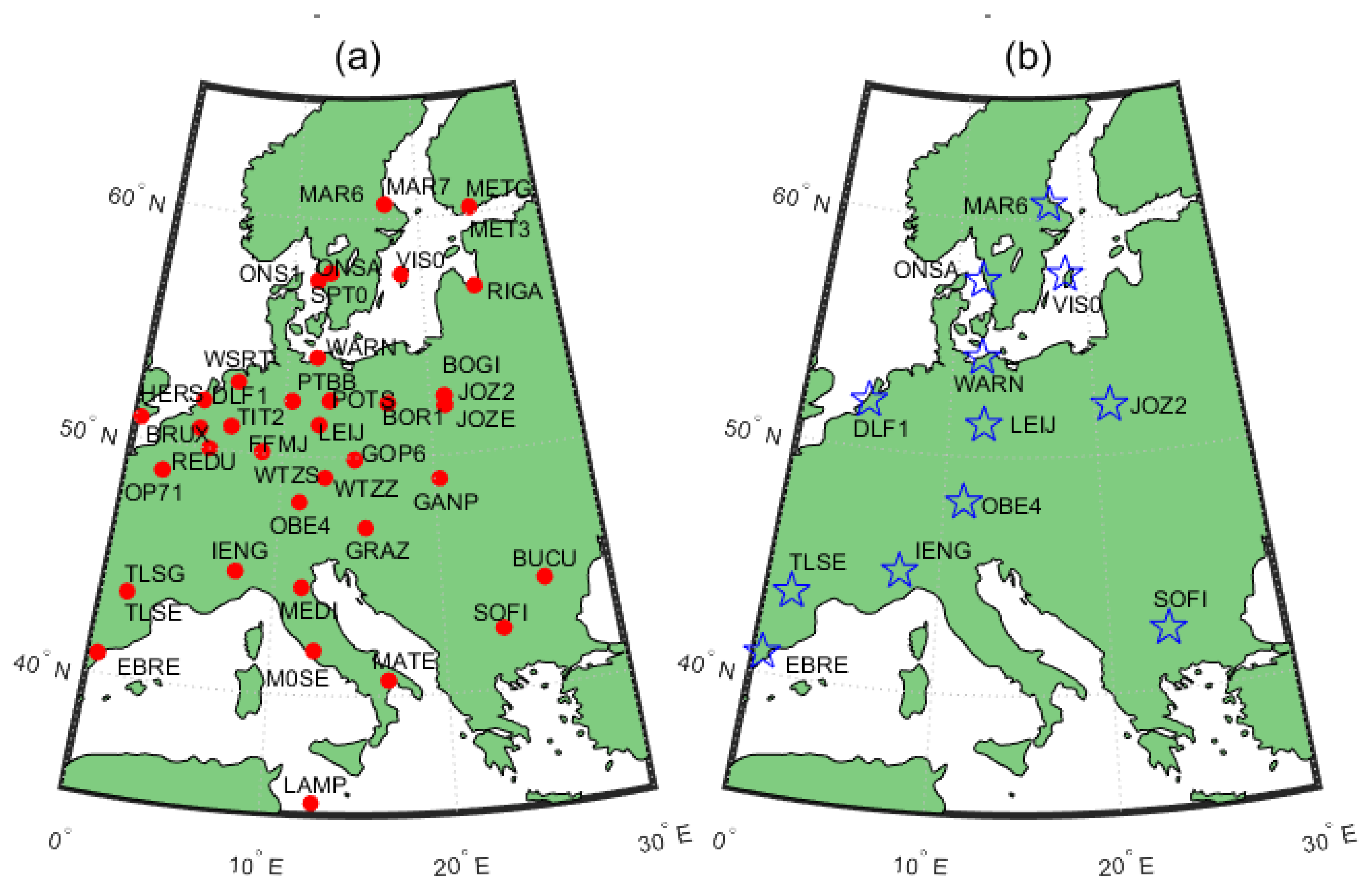
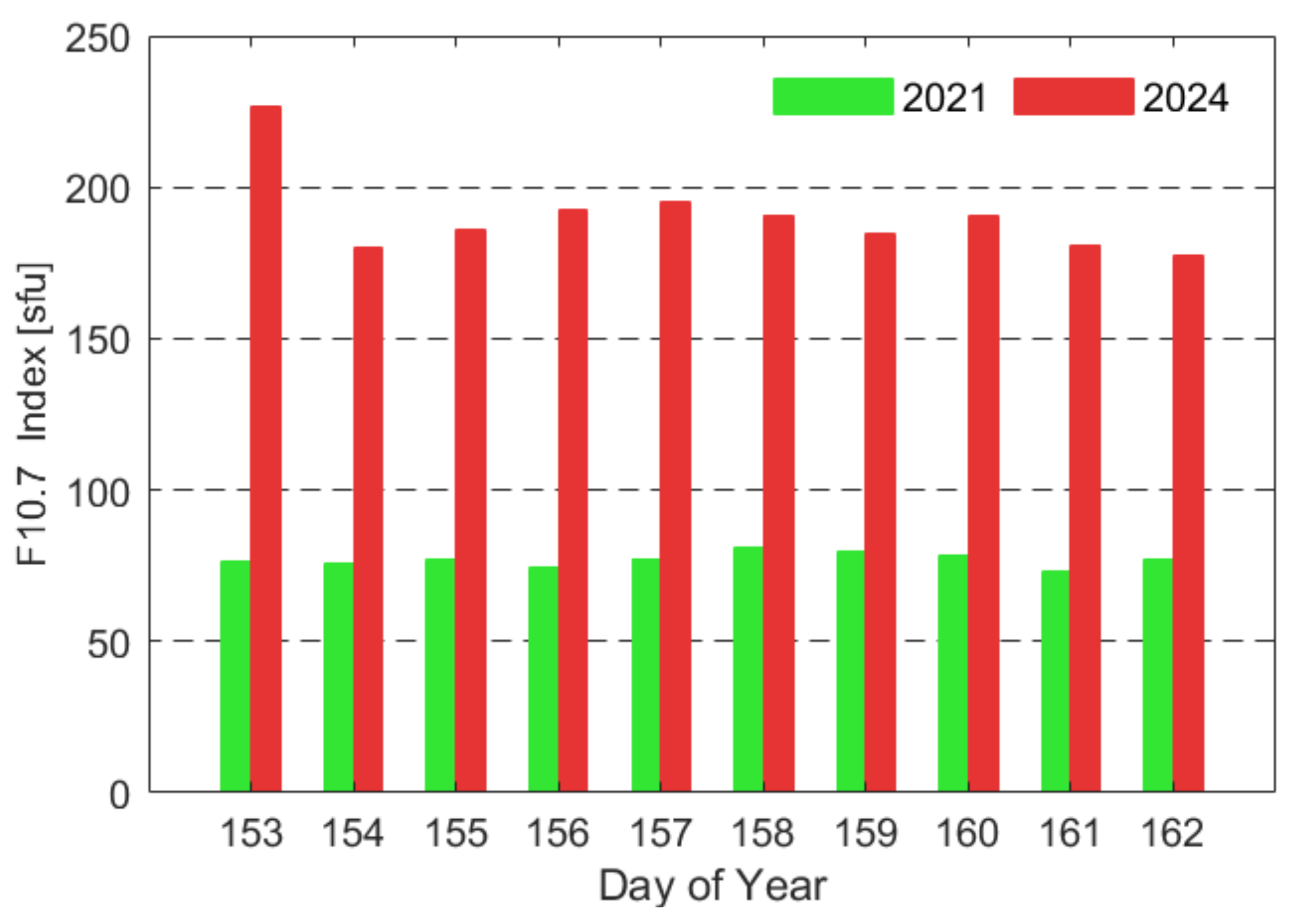
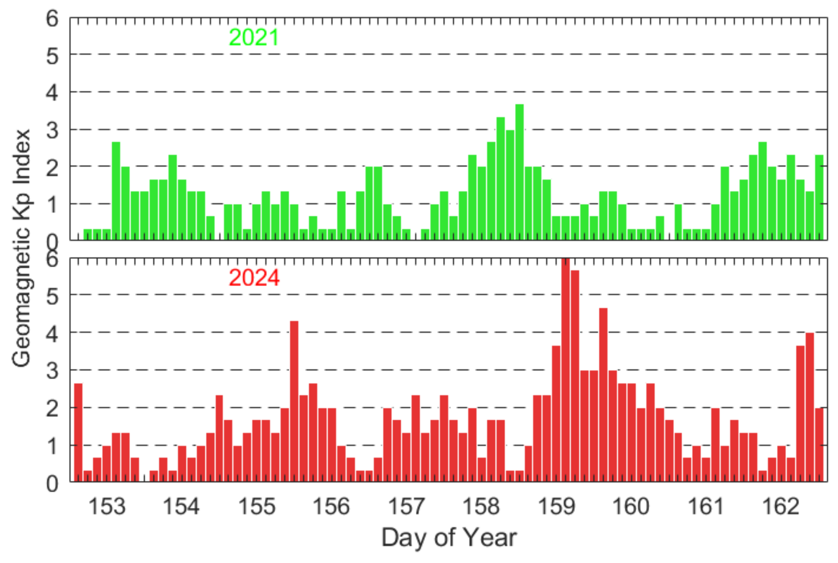
3.1. Experimental Data

Forty-one multi-GNSS experiment (MGEX) stations located in Europe are used to establish the regional ionospheric VTEC model. This experimental area covers a northern latitude of 35–65 degrees and an eastern longitude of 0–30 degrees. The distribution of all selected stations marked in red is displayed in Figure 1a. Twelve well-distributed blue stations (as shown in Figure 1b) in this monitoring network are used for testing the IW SFPPP performance and evaluating the external accord accuracy of the regional ionospheric VTEC model.

When selecting the ionospheric modeling time, we considered different solar and geomagnetic activity during solar cycle 25. Figure 2 shows the solar radio flux at 10.7 cm wavelength (download link: https://wdc.kugi.kyoto-u.ac.jp/kp/index.html#LIST (accessed on 8 February 2025)) during the two periods. The day of year (DoY) 153–162 in 2021 corresponds to the quiet period with the F10.7 index between 73.3 and 80.8 sfu (solar flux units), while in 2024, its F10.7 index varies from 177.8 to 226.9 sfu. This indicates that the solar activity in 2024 is particularly active. On the other hand, the geomagnetic Kp index (download link: https://wdc.kugi.kyoto-u.ac.jp/wdc/Sec3.html (accessed on 8 February 2025)) during the same period is shown in Figure 3. Most Kp index values in 2021 can be kept within 1–2 and no more than 3.67, indicating calm geomagnetic activity. In contrast, the Kp index in 2024 is higher, with several peaks exceeding 5, reflecting the active state of the ionosphere during this period.

3.2. Processing Strategies

In regional ionospheric VTEC modeling based on the IW SFPPP method, the adopted SF observations are C1W/L1C for GPS, C1C/L1C and C1X/L1X for Galileo, and C2I/L2I for BDS-3. For the traditional CCL method, the C1W/L1C+C2W/L2W observations of GPS, C1C/L1C+C5Q/L5Q and C1X/L1X+C5X/L5X observations of Galileo, and C2I/L2I+C6I/L6I observations of BDS-3 are used. In the process of both IW SFPPP and regional ionospheric modeling, the elevation cutoff angle is set to 10 degrees. The priori precision of the code and carrier-phase observations for GPS/Galileo/BDS-3 is set to 0.3 and 0.003 m, respectively, and the elevation-dependent model is used to weight observations of each satellite [33]. The GBM precise ephemeris provided by the Deutsches GeoForschungsZentrum (GFZ) was used to fix the satellite orbits and clocks. The precise coordinates of the MGEX stations used are fixed using the SINEX (Solution-INdependent EXchange) products. The relativistic effects, solid/ocean/polar tidal errors, and phase windup are corrected with traditional models [34,35]. In addition, the main processing strategies and adopted models are summarized in

Table 1. Processing strategies of the multi-GNSS IW SFPPP and regional ionospheric modeling.

Items	Strategies
I: IW SFPPP processing
Estimator	Kalman filter
Satellite/receiver antenna center offsets and variations	Corrected with igs20_2317.atx products
Satellite DCB	Corrected with CAS daily BSX products
Tropospheric delay	Dry delay: corrected with GPT2w+SAAS+VMF models Wet delay: estimated as random-walk process [36]
Ionospheric delay	Estimated as random-walk process [37]
Receiver clock	Estimated as white noise
Galileo and BDS-3 ISB	Estimated as random-walk process [38]
Phase ambiguity	Estimated as float solution
II: Regional ionospheric VTEC modeling
Estimator	Sequential least-squares adjustment
VTEC modeling algorithm	Polynomial function (6 orders × 4 degrees, 2 h interval)
Receiver DCB	Estimated as constant

.

4. Results and Discussion

The static positioning performance of GPS/Galileo/BDS-3 integrated IW SFPPP needs to be investigated. It can indirectly reflect the feasibility of the proposed ionospheric extraction method. To objectively evaluate the advantages of this novel method, the ionospheric model established by the IW SFPPP method was compared with the CODE GIM product and the CCL-based model. In addition, the external accord accuracy of the new method was also evaluated using the epoch-differenced GF combinations as reference.

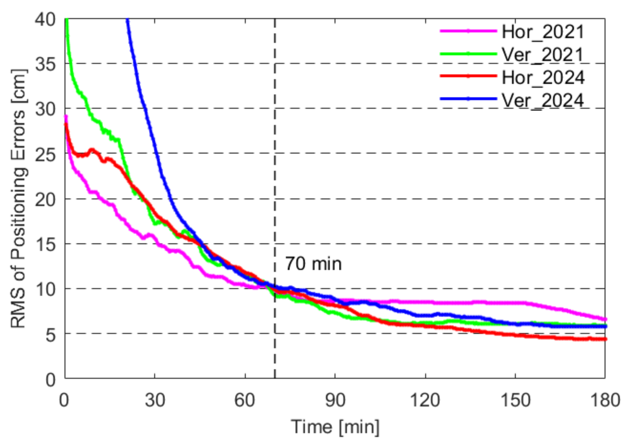
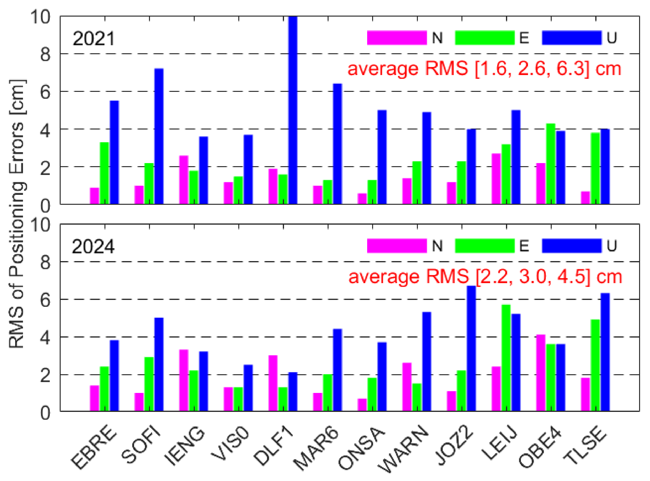
4.1. Performance of the Multi-GNSS Ionosphere-Weighted Single-Frequency PPP

The twelve blue stations shown in Figure 1b were selected for conducting the multi-GNSS IW SFPPP in static mode. The RMS values of positioning errors for all stations within 10 days are displayed in Figure 4. The abbreviations ‘Hor’ and ‘Ver’ in this figure denote the horizontal and vertical components. Both horizontal and vertical positioning errors of the GPS+Galileo+BDS-3 IW SFPPP in 2021 and 2024 can be less than 10 cm within about 70 min. After converging to 10 cm, the horizontal positioning errors in 2021 are significantly larger than those in 2024, mainly due to the smaller number of available BDS-3 satellites in 2021. In 2024, the positioning errors of both horizontal and vertical components can stabilize at 5 cm after 150 min.

Figure 5 gives the RMS positioning accuracy of the static multi-GNSS IW SFPPP after 3 h convergence for all tested stations. The positioning accuracy of most stations in 2024 is better than that in 2021, especially in the vertical direction. The mean RMS errors of all stations in 2021 can reach 1.6, 2.6, and 6.3 cm in the north (N), east (E), and up (U) directions, respectively. By comparison, the vertical positioning accuracy in 2024 has improved from 6.3 to 4.5 cm. This indicates that the current SFPPP through the multi-GNSS fusion and IW constraints can achieve high-precision positioning results, with horizontal results better than 3 cm and vertical results better than 5 cm. Therefore, it can be proven that the multi-GNSS IW SFPPP method for extracting ionospheric observables is theoretically feasible. More importantly, the monitoring station coordinates are fixed using the SINEX solutions instead of being estimated as parameters, which will further improve the accuracy of extracting ionospheric observables.

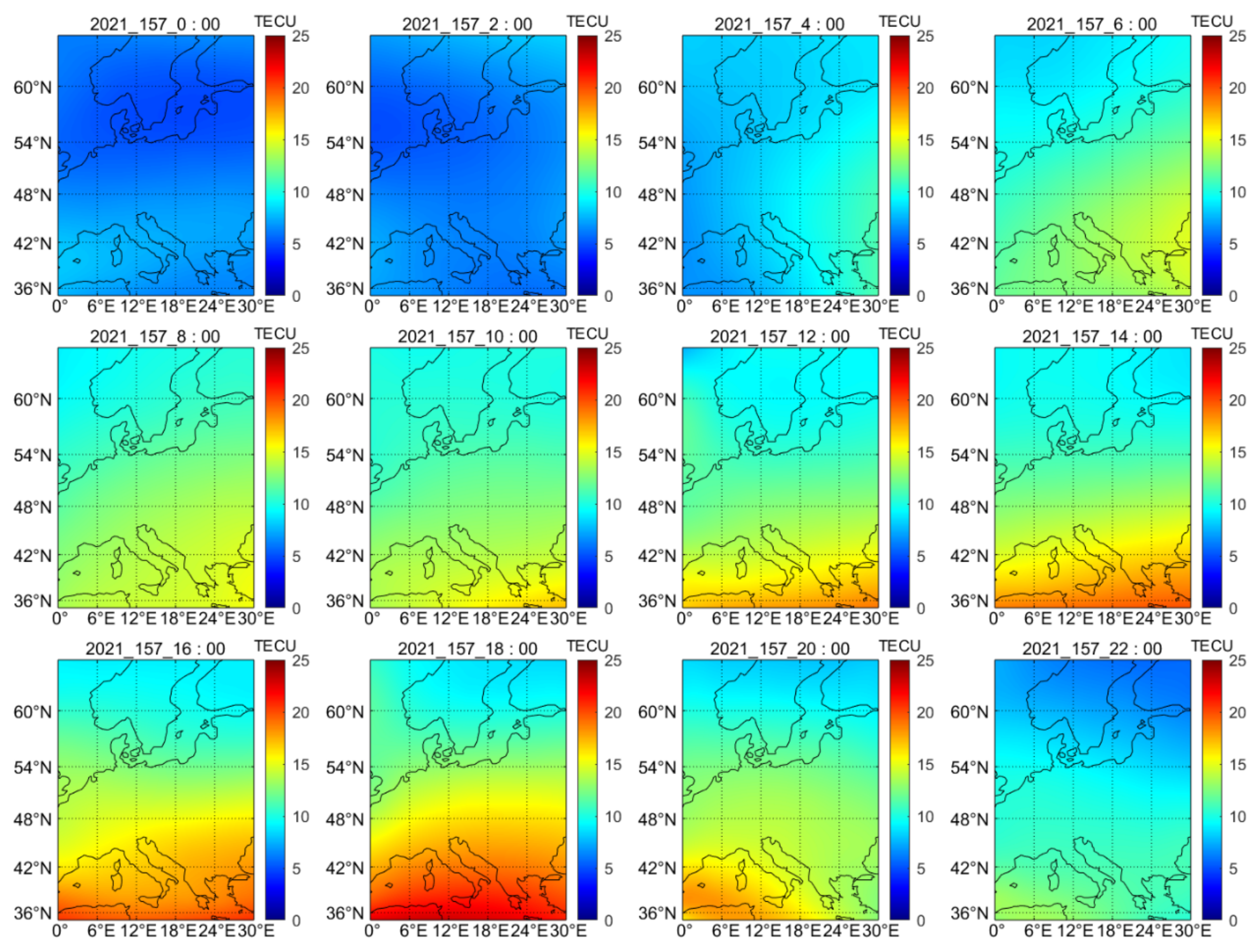
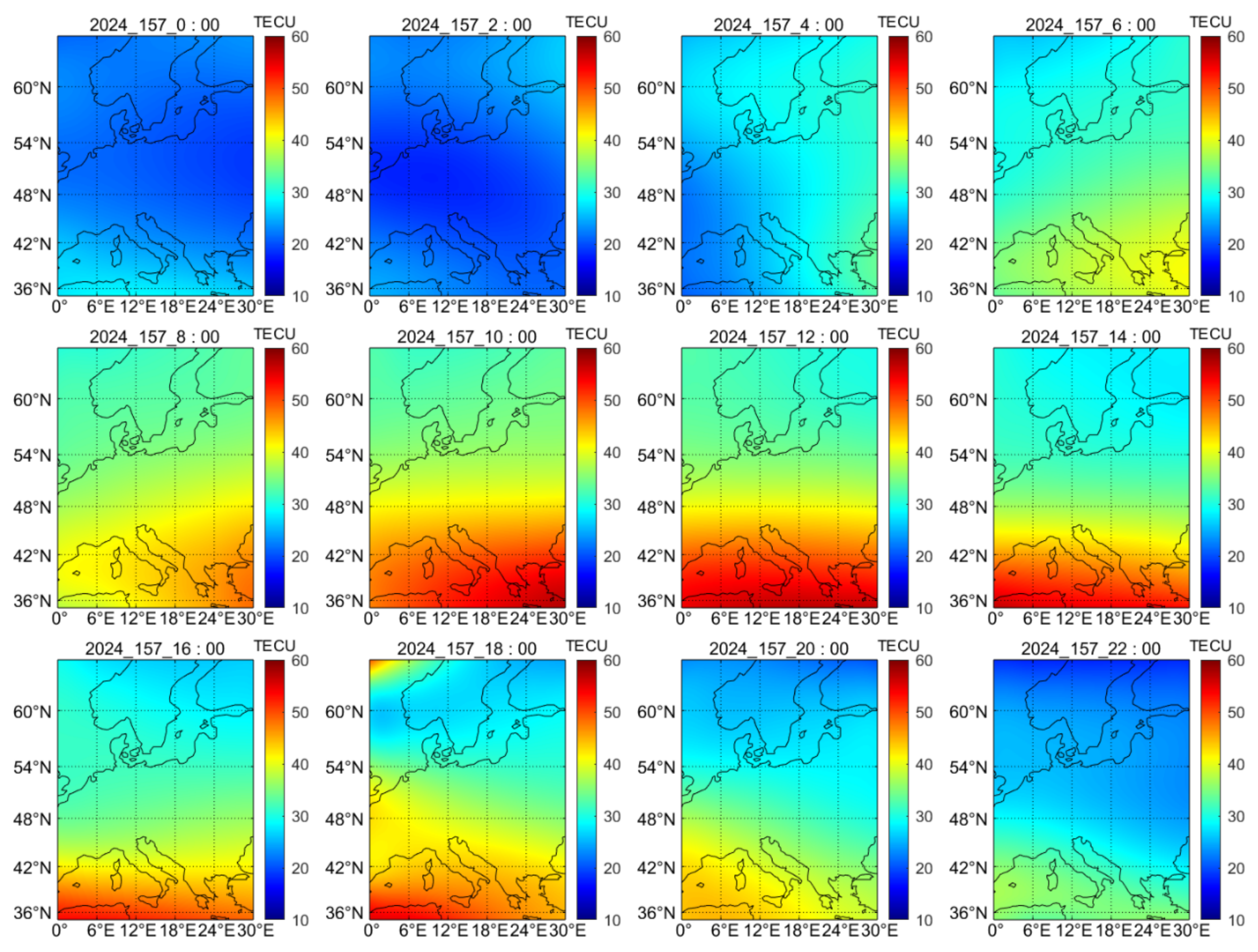
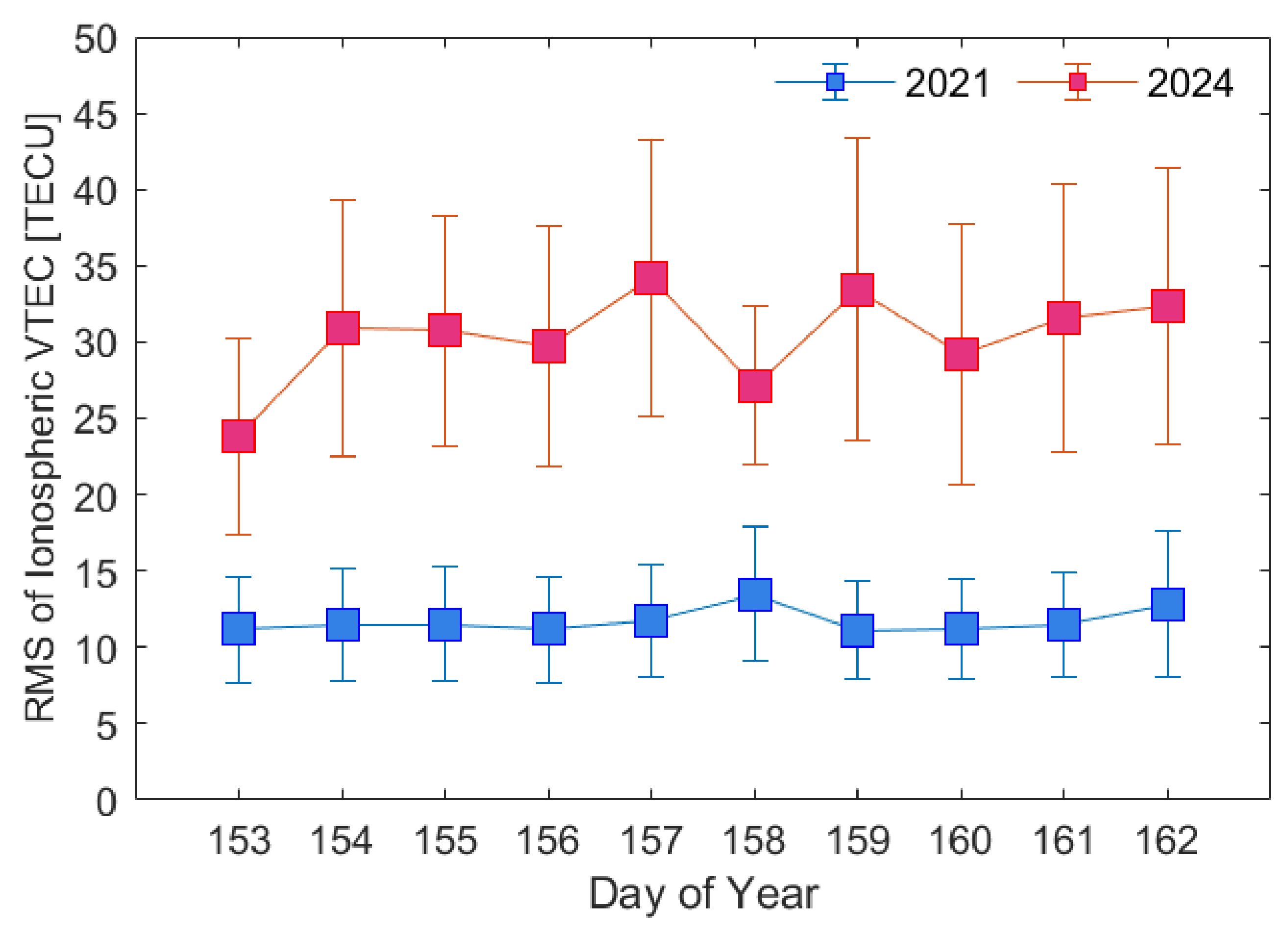
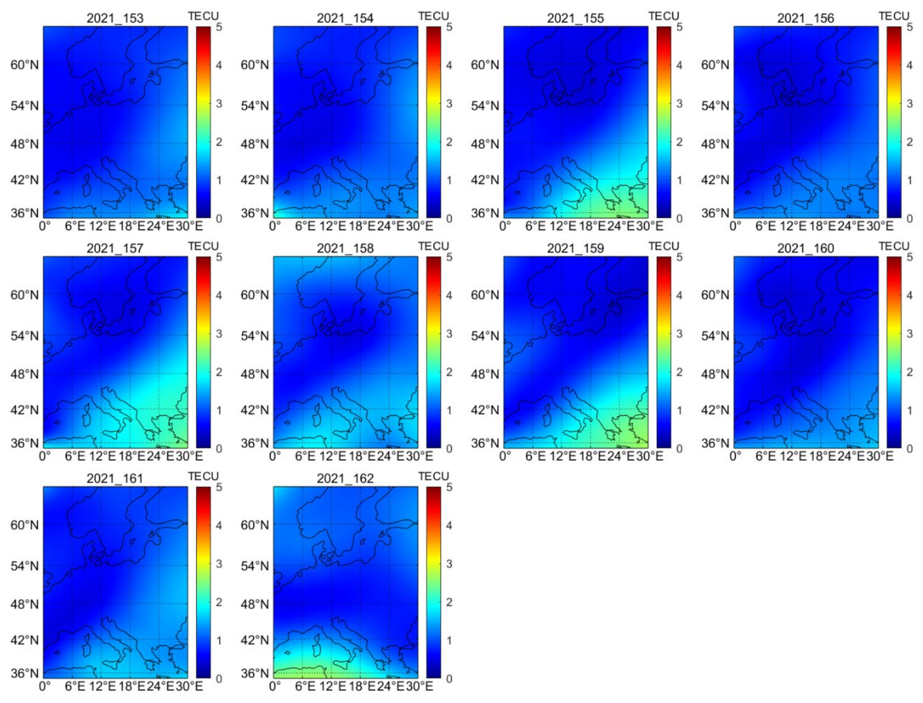
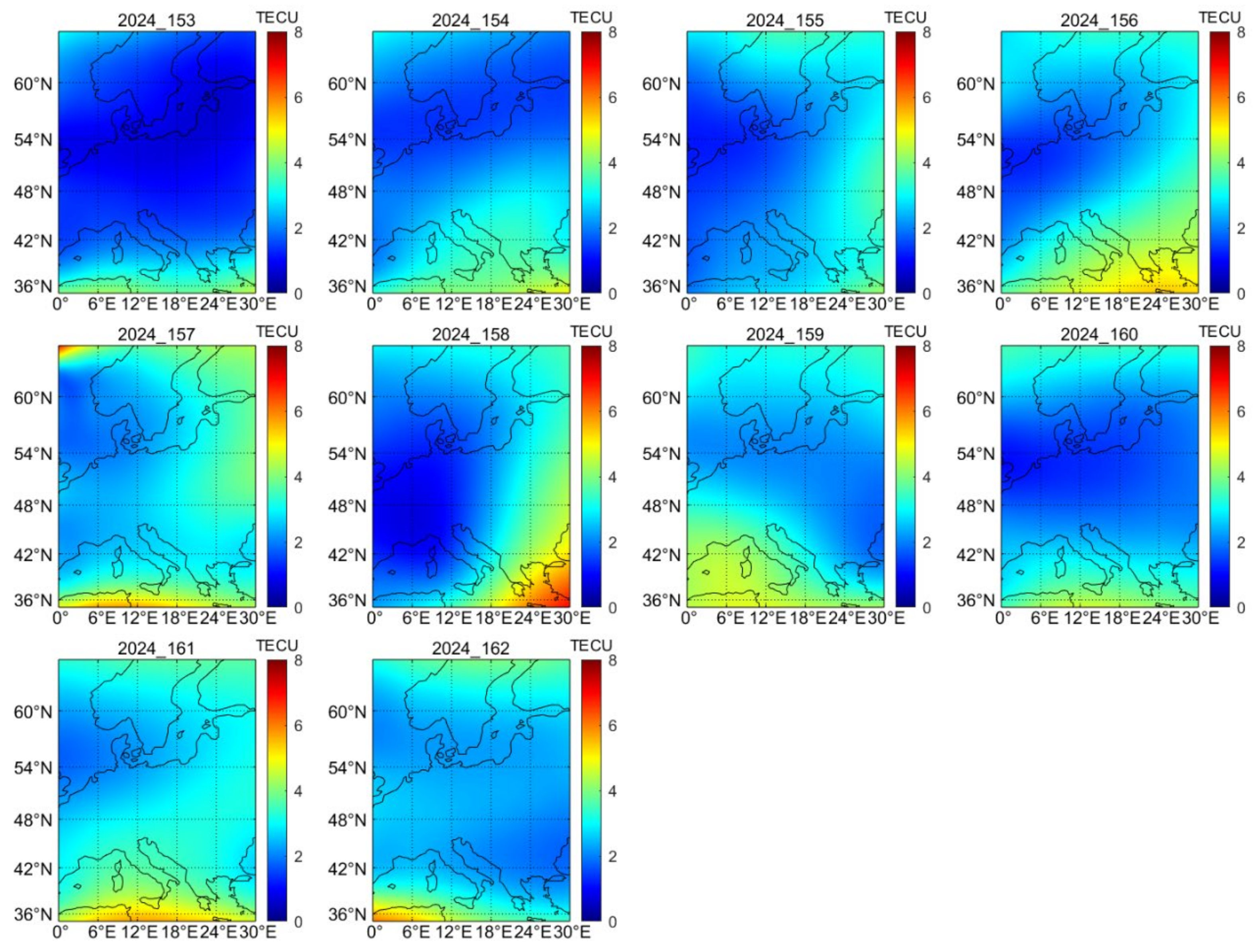
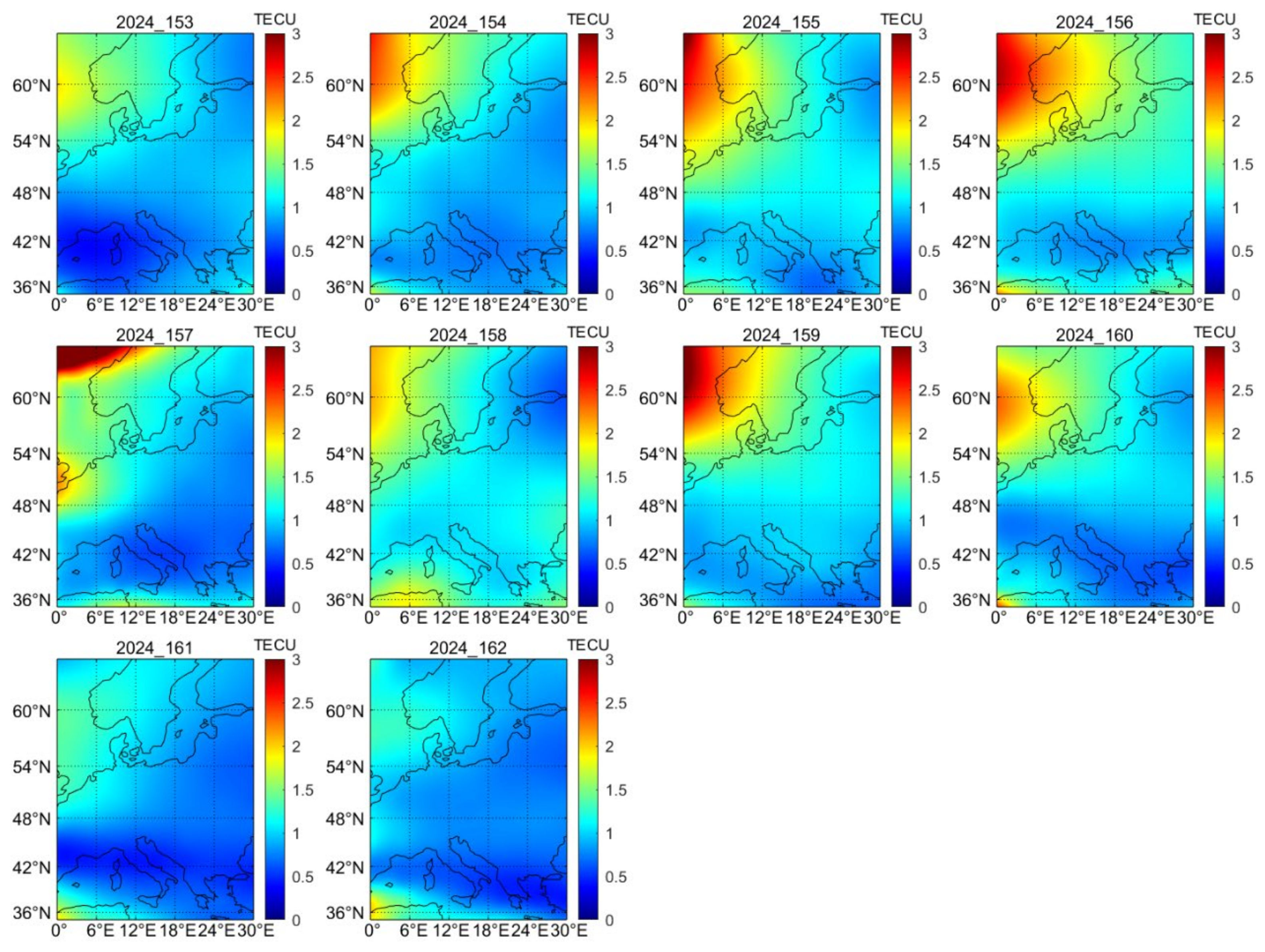
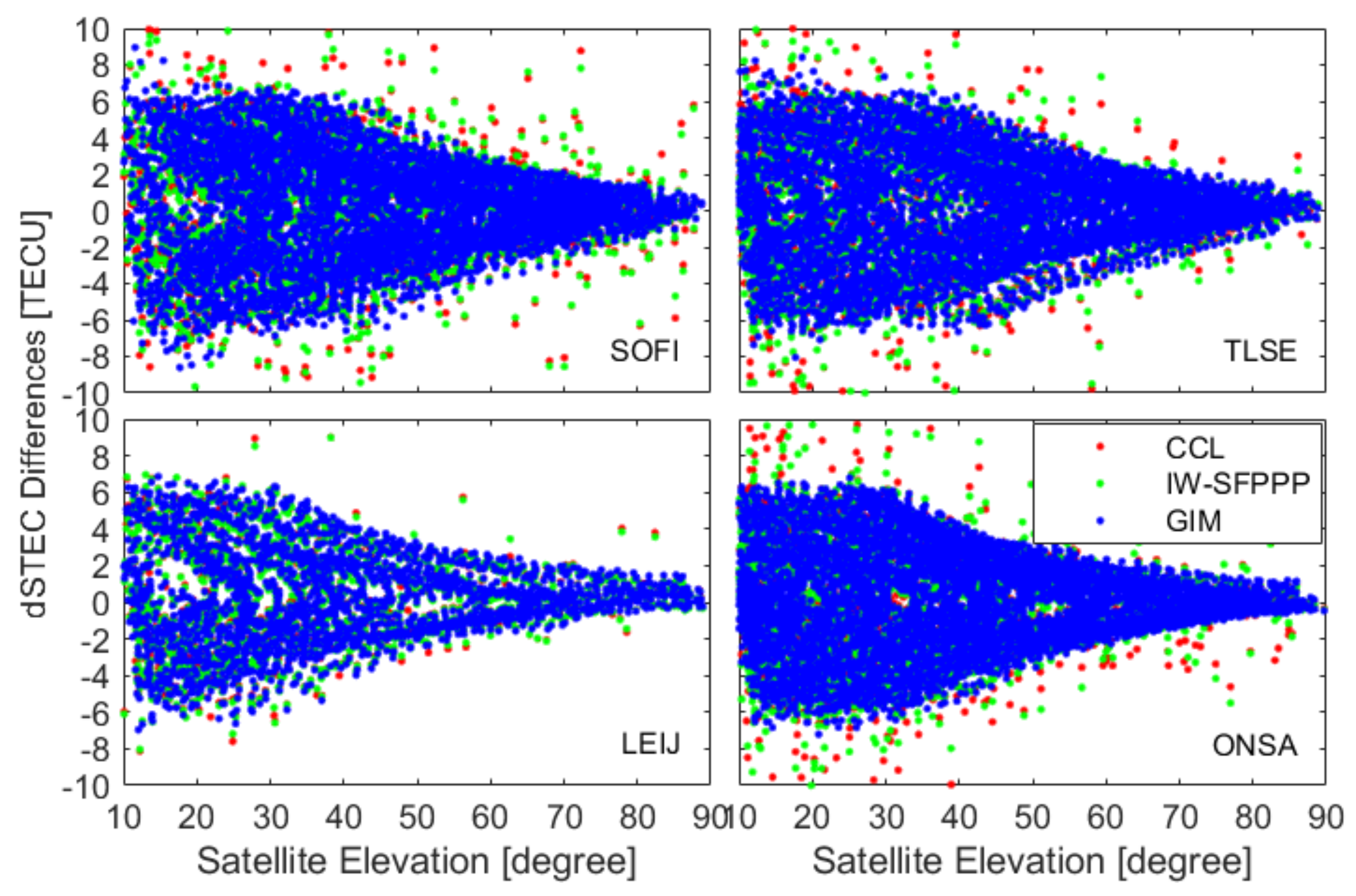
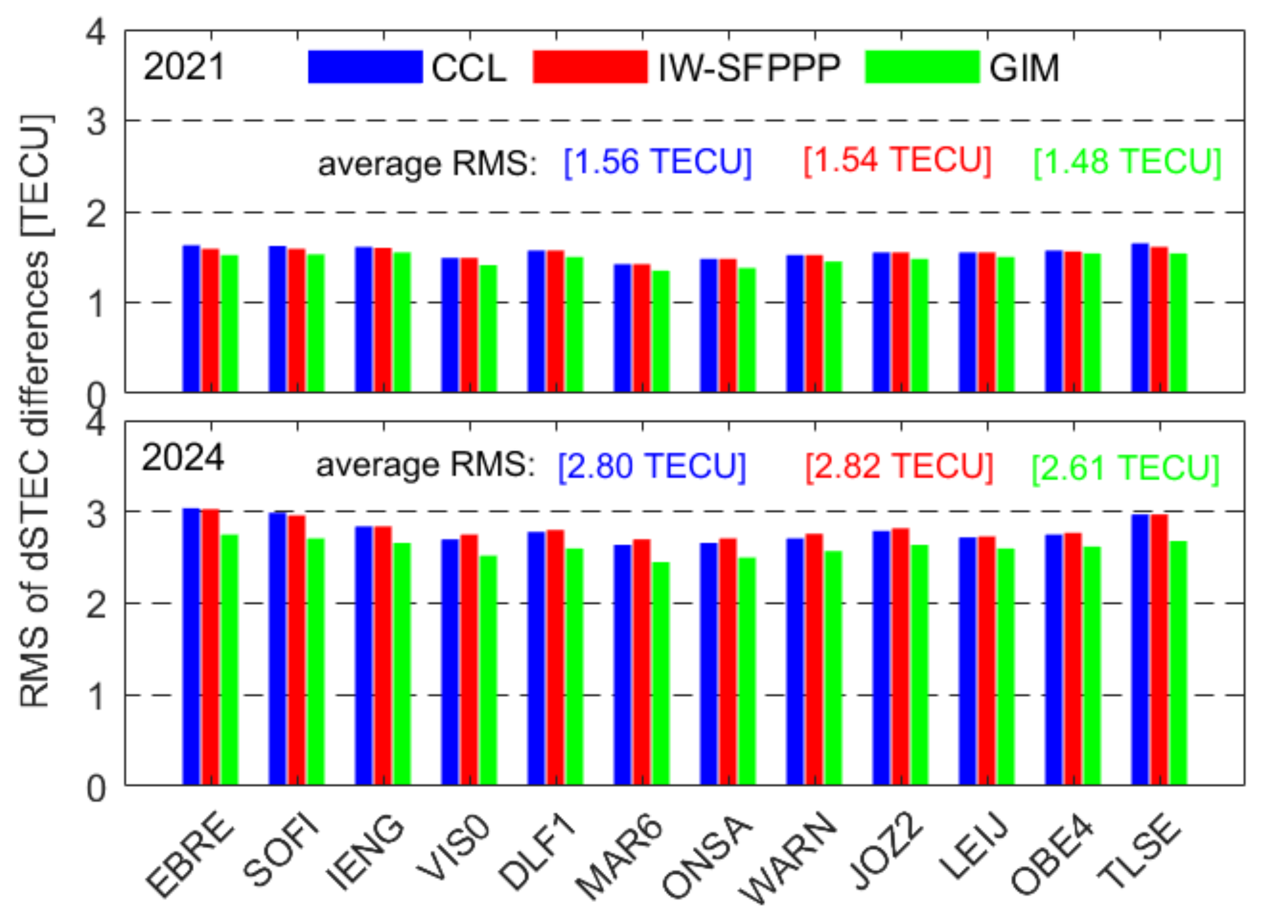
4.2. Quality Assessment of the Regional Ionospheric VTEC Model in Comparison with GIM

In this study, 35 coefficients (6 orders and 4 degrees in polynomial function) of the regional ionospheric VTEC model are estimated with an interval of 2 h. Figure 6 shows the gridded ionospheric VTEC maps with the spatial resolution of 0.1° × 0.1° on DoY 157, 2021, which are calculated from the IW SFPPP-derived slant ionospheric observables. We can see that the daily VTEC values are no more than 25 TECU, and some values can even be less than 5 TECU at GPS time (GPST) 00:00 and 02:00. This indicates that the ionospheric VTEC values in low-solar-activity years (seen in Figure 2) are also relatively small. There are significant differences in VTEC values at different latitudes, with VTEC in higher-latitude areas generally smaller than those in lower-latitude areas. The same processing is applied to the regional ionospheric VTEC maps on DoY 157, 2024, and the corresponding results are given in Figure 7. Due to the high solar activity in 2024, the peak of VTEC values in daily solutions can reach up to 60 TECU and its minimum value exceeds 10 TECU. Under this ionospheric condition, the differences in ionospheric VTEC between different latitude bands are quite distinct.

Figure 8 summarizes the RMS of ionospheric VTEC values derived from the IW SFPPP method. The error bars in this figure represent the STD of ionospheric VTEC values. The ionospheric VTEC values in 2024 with about 30 TECU are much larger than those in 2021 with about 12 TECU, which is consistent with the trend of the F10.7 index during the same period (seen in Figure 2). From the results of the error bars, it can be seen that the mean STD of ionospheric VTEC in 2024 can reach 8 TECU, while in 2021, the corresponding statistical value is around 3.7 TECU. This proves that the ionospheric VTEC in 2024 have greater variation amplitude in daily solutions.

In this section, the post-processing GIM products provided by CODE are used to judge the quality of the regional ionospheric VTEC models. The comparison interval is set to 2 h, and every day has 12 groups of VTEC differences (i.e., dVTEC) between the regional ionospheric VTEC and final GIM products. Figure 9 and Figure 10 show the RMS maps of dVTEC on DoY 153-162 in 2021 derived from the IW SFPPP and CCL methods, respectively. It can be seen that the RMS values of most dVTEC for the IW SFPPP method are better than 1 TECU and have good consistency in spatial distribution. For the CCL method, the RMS peak of dVTEC on DoY 153-155 and 160 may reach up to 5 TECU, which may be attributed to the sparsely distributed monitoring stations in these areas. By comparing Figure 9 and Figure 10, we can see that using the IW SFPPP method to construct the regional ionospheric VTEC model can achieve better performance in areas with sparse stations.

The same comparative strategies are applied to the high-solar-activity year of 2024. The corresponding RMS maps of dVTEC generated by the IW SFPPP and CCL methods are presented in Figure 11 and Figure 12, respectively. The variation amplitude of the daily dVTEC solutions in 2024 is more intense than that in 2021, with peak values of up to 8 TECU, which is reasonable given that ionospheric VTEC is more difficult to model under high solar and geomagnetic conditions. The majority of dVTEC values of the IW SFPPP method are significantly lower than those of the CCL method on DoY 155–156 and 159–160. More than half of dVTEC for the IW SFPPP can be less than 3 TECU in daily solutions, while for the CCL method, the corresponding dVTEC values are kept within 3 to 5 TECU. This proves that the IW SFPPP method still outperforms the CCL method in high-solar-activity years.

Figure 13 summarizes the RMS values of VTEC differences between the regional ionospheric model and final GIM products on different days. Compared with the CCL method with a mean RMS of 1.32 TECU in 2021, the corresponding accuracy of dVTEC based on the IW SFPPP method can be improved by 17.4% to 1.09 TECU. In the high-solar-activity year of 2024, the modeling precision of the regional ionospheric VTEC sharply decreased, and its mean RMS values of dVTEC are reduced to 2.83 and 3.24 TECU for the IW SFPPP and CCL methods, respectively. The improvement in dVTEC accuracy using the IW SFPPP method is about 12.7% compared with the CCL method. No matter what the solar and geomagnetic activity conditions are, the conformity between the regional ionospheric VTEC modeled by the IW SFPPP method and final GIM products is significantly better than that of the CCL method.

In order to more intuitively reflect the differences between the IW SFPPP and CCL methods in regional ionospheric VTEC modeling, the RMS maps of dVTEC derived from the two abovementioned methods in 2021 and 2024 are shown in Figure 14 and Figure 15, respectively. Most dVTEC values in 2021 are under 1 TECU, while in 2024, the corresponding values vary between 1 and 2 TECU. This indicates that the difference in modeling accuracy between the IW SFPPP and CCL methods may be increased as solar activity strengthens. In both low- and high-solar-activity years, the larger differences in dVTEC are presented in areas with sparse monitoring stations and their maximum values can be up to 3 TECU. The main reason for this phenomenon may be that the CCL method has fewer IPPs in sparse areas after removing gross errors. The IW SFPPP method with a large number of IPPs can demonstrate superior performance in areas with sparse monitoring stations. Figure 16 gives the RMS of VTEC differences between the IW SFPPP and CCL methods on each test day. We can see that the mean RMS of dVTEC values for all test days is 0.72 and 1.06 TECU in 2021 and 2024, respectively. This illustrates the conformity of VTEC for the two methods in 2021 is better than that in 2024, as the ionospheric VTEC can be more precisely modeled in calm solar and geomagnetic activity.

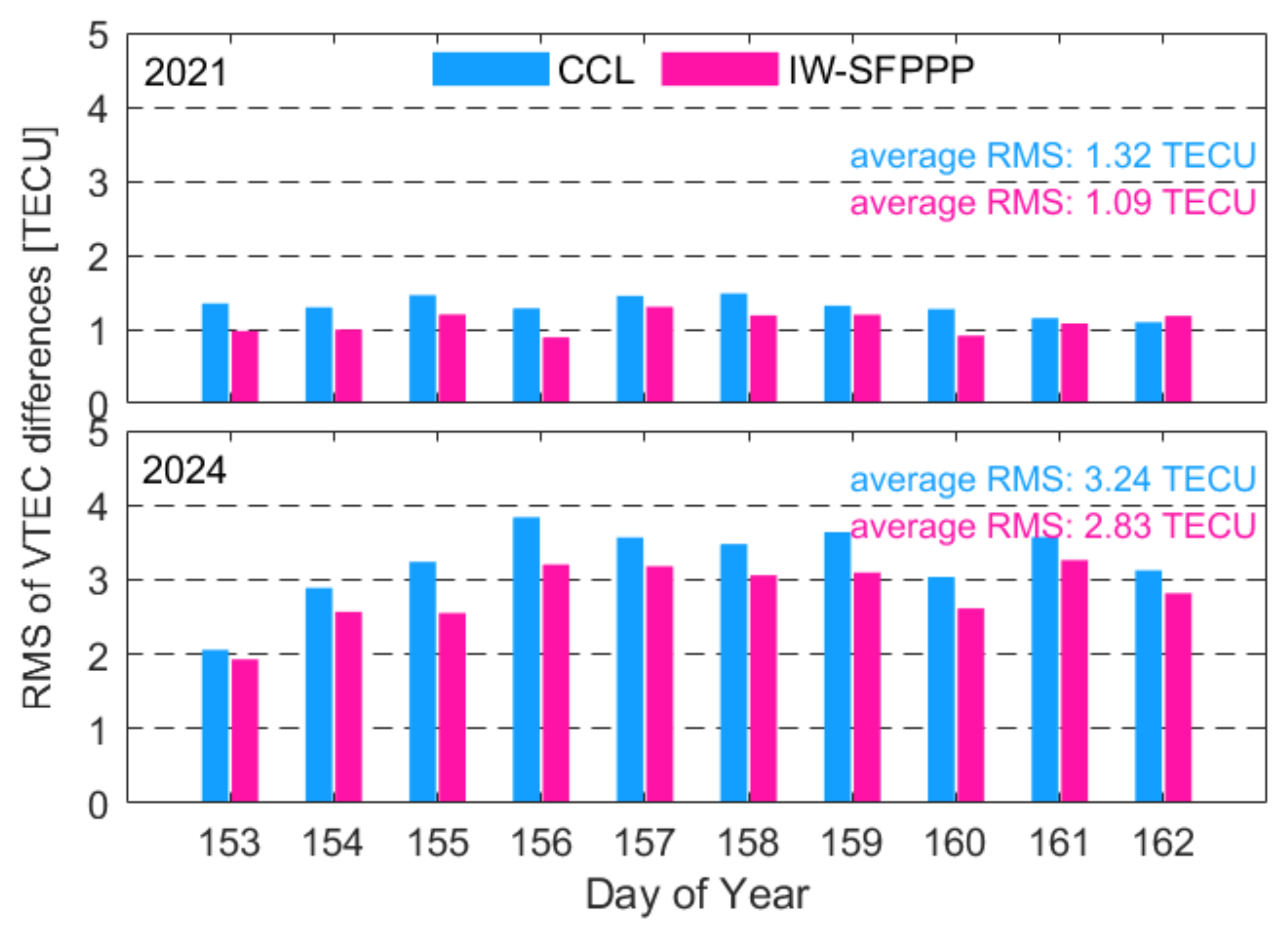
4.3. Evaluation of External Accord Accuracy for Regional Ionospheric VTEC Model

Considering that the epoch-differenced GF combinations of carrier-phase observations have the ability to obtain the mm level STEC variations (i.e., dSTEC), the dSTEC can be adopted as the referenced values to verify the external accord accuracy of different ionospheric VTEC models [39]. The dSTEC modeled values corresponding to the above dSTEC referenced values are calculated from different regional ionospheric VTEC models (IW SFPPP and CCL methods) and CODE final GIM products. Thus, the dSTEC differences can be defined as the dSTEC modeled values minus the dSTEC reference values. In this section, twelve well-distributed stations marked in blue, as shown in Figure 1b, are used to implement the dSTEC comparison. The sampling rate of dSTEC is set to 5 min. Figure 17 and Figure 18 show the dSTEC differences in four representative stations on DoY 157 in 2021 and 2024, respectively. It can be seen that dSTEC differences in 2024 are significantly larger than those in 2021 for both regional and global ionospheric VTEC models, which is caused by the larger ionospheric delays and drastic changes during high-solar-activity years. As the satellite elevation increases, the dSTEC differences sharply decrease. When the satellite elevation is higher than 40 degrees, the dSTEC differences in 2021 can be maintained within 4 TECU, but in 2024, the corresponding value is increased to 6 TECU. On the other hand, the distribution of dSTEC differences for both IW SFPPP and CCL methods is not as concentrated as for GIM products. This indicates that the quality of the final GIM products is slightly better than that of the regional ionospheric VTEC models established in this contribution.

Figure 19 gives the RMS of dSTEC differences for the IW SFPPP, CCL, and GIM models on DoY 153–162 in 2021 and 2024. The mean RMS values of dSTEC differences in 2021 are 1.54, 1.56, and 1.48 TECU for the IW SFPPP method, CCL method, and GIM products, respectively. In the high-solar-activity year of 2024, the corresponding values are increased to 2.82, 2.80, and 2.61 TECU, respectively. By evaluating the external accord accuracy of different ionospheric VTEC models, the quality of the regional ionospheric VTEC model established by the IW SFPPP method can be fully comparable to that of the CCL method, and its accuracy difference with the final GIM products can be maintained within 0.2 TECU.

5. Conclusions

The classical CCL method, a commonly used technique for extracting ionospheric observables, has ideal performance and reliability. However, it must rely on DF receivers, which results in high hardware costs for ionospheric modeling. Considering that current UU-SFPPP can achieve a positioning accuracy that is better than 5 cm with the combination of multi-GNSS and external ionospheric constraints, the multi-GNSS IW SFPPP can be expected to become a high-precision and low-cost method for extracting ionospheric observables. In order to investigate the advantages of this novel STEC extraction method in regional ionospheric modeling, forty-one MGEX stations located in Europe are used to establish ionospheric models, and both low- and high-solar-activity conditions are considered.

Using the VTEC provided by the final CODE GIM as a reference, the regional ionospheric model based on the IW SFPPP method has a significantly better VTEC accuracy than the CCL method. In the low-solar-activity year of 2021, compared with the CCL method, the RMS VTEC accuracy of the IW SFPPP method can be improved by 17.4% to 1.09 TECU, while in the high-solar-activity year of 2024, the corresponding improvement ratio is about 12.7% for the IW SFPPP method. From the daily solutions of the VTEC difference between the regional ionospheric model and final GIM products, the modeling accuracy of the IW SFP method in areas with sparse monitoring stations is better than that of the CCL method. In addition, in the direct comparison between the IW SFPPP and CCL methods, the RMS of VTEC differences in 2021 and 2024 is about 0.72 and 1.06 TECU, respectively.

In the external accord accuracy evaluation of the regional ionospheric models, the GNSS dSTEC with mm level accuracy is adopted as the reference value. Regardless of the strength of solar activity, the accuracy of dSTEC differences for the IW SFPPP method is comparable to that of the CCL method, and its RMS values are about 1.5 and 2.8 TECU in 2021 and 2024, respectively. This indicates that the proposed IW SFPPP method using only SF observations can achieve the same ionospheric modeling accuracy as the CCL method with DF observations. However, this novel method only uses observations from high-precision geodetic GNSS receivers for testing, and the quality of SF observations is significantly better than that of low-cost GNSS receivers. To further validate the feasibility and advantages of the proposed method in truly low-cost ionospheric modeling, the future work will focus on the performance evaluation of low-cost GNSS monitoring networks.

References

1. Feltens, J. The activities of the ionosphere working group of the International GPS Service (IGS). GPS Solut. 2003, 7, 41–46. [Google Scholar] [CrossRef]
2. Hernandez-Pajares, M.; Juan, J.M.; Sanz, J.; Aragon-Angel, A.; Garcia-Rigo, A.; Salazar, D.; Escudero, M. The ionosphere: Effects, GPS modeling and the benefits for space geodetic techniques. J. Geod. 2011, 85, 887–907. [Google Scholar] [CrossRef]
3. de Bakker, P.F.; Tiberius, C.C.J.M. Real-time multi-GNSS single-frequency precise point positioning. GPS Solut. 2017, 21, 1791–1803. [Google Scholar] [CrossRef]
4. Odolinski, R.; Teunissen, P.J.G. An assessment of smartphone and low-cost multi-GNSS single-frequency RTK positioning for low, medium and high ionospheric disturbance periods. J. Geod. 2018, 93, 701–722. [Google Scholar] [CrossRef]
5. Wang, A.; Zhang, Y.; Chen, J.; Wang, H.; Yuan, D.; Jiang, J.; Zhang, Z. Investigating the contribution of BDS-3 observations to multi-GNSS single-frequency precise point positioning with different ionospheric models. Adv. Space Res. 2024, 73, 553–570. [Google Scholar] [CrossRef]
6. Cahuasquí, J.A.; Hoque, M.M.; Jakowski, N. Positioning performance of the Neustrelitz total electron content model driven by Galileo Az coefficients. GPS Solut. 2022, 26, 93. [Google Scholar] [CrossRef]
7. Liu, Z.; Yang, Z. Anomalies in broadcast ionospheric coefficients recorded by GPS receivers over the past two solar cycles (1992–2013). GPS Solut. 2016, 20, 23–37. [Google Scholar] [CrossRef]
8. Klobuchar, J.A. Ionospheric time-delay algorithm for single-frequency GPS users. IEEE Trans. Aerosp. Electron. Syst. 1987, 23, 325–331. [Google Scholar] [CrossRef]
9. Montenbruck, O.; González Rodríguez, B. NeQuick-G performance assessment for space applications. GPS Solut. 2019, 24, 13. [Google Scholar] [CrossRef]
10. Yuan, Y.; Wang, N.; Li, Z.; Huo, X. The BeiDou global broadcast ionospheric delay correction model (BDGIM) and its preliminary performance evaluation results. Navigation 2019, 66, 55–69. [Google Scholar] [CrossRef]
11. Wang, A.; Chen, J.; Zhang, Y.; Meng, L.; Wang, B.; Wang, J. Evaluating the impact of CNES real-time ionospheric products on multi-GNSS single-frequency positioning using the IGS real-time service. Adv. Space Res. 2020, 66, 2516–2527. [Google Scholar] [CrossRef]
12. Liu, H.; Ren, X.; Xu, G. Investigating the performance of IGS real-time global ionospheric maps under different solar conditions. Remote Sens. 2023, 15, 4661. [Google Scholar] [CrossRef]
13. Roma-Dollase, D.; Hernández-Pajares, M.; Krankowski, A.; Kotulak, K.; Ghoddousi-Fard, R.; Yuan, Y.; Li, Z.; Zhang, H.; Shi, C.; Wang, C.; et al. Consistency of seven different GNSS global ionospheric mapping techniques during one solar cycle. J. Geod. 2018, 92, 691–706. [Google Scholar] [CrossRef]
14. Rovira-Garcia, A.; Juan, J.; Sanz, J.; Gonzalez-Casado, G.; Ibanez, D. Accuracy of ionospheric models used in GNSS and SBAS: Methodology and analysis. J. Geod. 2016, 90, 229–240. [Google Scholar] [CrossRef]
15. Liu, T.; Zhang, B.; Yuan, Y.; Li, M. Real-time precise point positioning (RTPPP) with raw observations and its application in real-time regional ionospheric VTEC modeling. J. Geod. 2018, 92, 1267–1283. [Google Scholar] [CrossRef]
16. Huo, X.; Long, Y.; Liu, H.; Yuan, Y.; Liu, Q.; Li, Y.; Liu, M.; Liu, Y.; Sun, W. A novel ionospheric TEC mapping function with azimuth parameters and its application to the Chinese region. J. Geod. 2024, 98, 13. [Google Scholar] [CrossRef]
17. Ciraolo, L.; Azpilicueta, F.; Brunini, C.; Meza, A.; Radicella, S. Calibration errors on experimental slant total electron content (TEC) determined with GPS. J. Geod. 2007, 81, 111–120. [Google Scholar] [CrossRef]
18. Ren, X.; Chen, J.; Li, X.; Zhang, X. Multi-GNSS contributions to differential code biases determination and regional ionospheric modeling in China. Adv. Space Res. 2020, 65, 221–234. [Google Scholar] [CrossRef]
19. Wang, J.; Huang, G.; Zhou, P.; Yang, Y.; Zhang, Q.; Gao, Y. Advantages of uncombined precise point positioning with fixed ambiguity resolution for slant total electron content (STEC) and differential code bias (DCB) estimation. Remote Sens. 2020, 12, 304. [Google Scholar] [CrossRef]
20. Zhang, B.; Ou, J.; Yuan, Y.; Li, Z. Extraction of line-of-sight ionospheric observables from GPS data using precise point positioning. Sci. China Earth Sci. 2012, 55, 1919–1928. [Google Scholar] [CrossRef]
21. Xiang, Y.; Gao, Y.; Shi, J.; Xu, C. Consistency and analysis of ionospheric observables obtained from three precise point positioning models. J. Geod. 2019, 93, 1161–1170. [Google Scholar] [CrossRef]
22. Ren, X.; Chen, J.; Li, X.; Zhang, X. Ionospheric total electron content estimation using GNSS carrier phase observations based on zero-difference integer ambiguity: Methodology and assessment. IEEE Trans. Geosci. Remote Sens. 2020, 59, 817–830. [Google Scholar] [CrossRef]
23. Wang, A.; Zhang, Y.; Chen, J.; Liu, X.; Wang, H. Regional real-time between-satellite single-differenced ionospheric model establishing by multi-GNSS single-frequency observations: Performance evaluation and PPP augmentation. Remote Sens. 2024, 16, 1511. [Google Scholar] [CrossRef]
24. Su, K.; Jin, S. A novel GNSS single-frequency PPP approach to estimate the ionospheric TEC and satellite pseudorange observable-specific signal bias. IEEE Trans. Geosci. Remote Sens. 2022, 60, 5801712. [Google Scholar] [CrossRef]
25. Zhao, C.; Yuan, Y.; Zhang, B.; Li, M. Ionosphere sensing with a low-cost, single-frequency, multi-GNSS receiver. IEEE Trans. Geosci. Remote Sens. 2019, 57, 881–892. [Google Scholar] [CrossRef]
26. Li, B.; Zang, N.; Ge, H.; Shen, Y. Single-frequency PPP models: Analytical and numerical comparison. J. Geod. 2019, 93, 2499–2514. [Google Scholar] [CrossRef]
27. Wang, N.; Yuan, Y.; Li, Z.; Montenbruck, O.; Tan, B. Determination of differential code biases with multi-GNSS observations. J. Geod. 2016, 90, 209–228. [Google Scholar] [CrossRef]
28. Wilgan, K.; Hadas, T.; Hordyniec, P.; Bosy, J. Real-time precise point positioning augmented with high-resolution numerical weather prediction model. GPS Solut. 2017, 21, 1341–1353. [Google Scholar] [CrossRef]
29. Chen, J.; Zhang, Y.; Yu, C.; Wang, A.; Song, Z.; Zhou, J. Models and performance of SBAS and PPP of BDS. Satell. Navig. 2022, 3, 4. [Google Scholar] [CrossRef]
30. Hernandez-Pajares, M.; Juan, J.M.; Sanz, J.; Orus, R.; Garcia-Rigo, A.; Feltens, J.; Komjathy, A.; Schaer, S.C.; Krankowski, A. The IGS VTEC maps: A reliable source of ionospheric information since 1998. J. Geod. 2009, 83, 263–275. [Google Scholar] [CrossRef]
31. Zhou, C.; Yang, L.; Li, B.; Balz, T. M_GIM: A MATLAB-based software for multi-system global and regional ionospheric modeling. GPS Solut. 2023, 27, 42. [Google Scholar] [CrossRef]
32. Sanz, J.; Miguel, J.J.; Rovira-Garcia, A.; Gonzalez-Casado, G. GPS differential code biases determination: Methodology and analysis. GPS Solut. 2017, 21, 1549–1561. [Google Scholar] [CrossRef]
33. Zhang, Y.; Chen, J.; Gong, X.; Chen, Q. The update of BDS-2 TGD and its impact on positioning. Adv. Space Res. 2020, 65, 2645–2661. [Google Scholar] [CrossRef]
34. Wu, J.T.; Wu, S.C.; Hajj, G.A.; Bertiger, W.I.; Lichten, S.M. Effects of antenna orientation on GPS carrier phase. Manuscr. Geod. 1993, 18, 91–98. [Google Scholar] [CrossRef]
35. Petit, G.; Luzum, B. IERS Conventions; IERS Technical 2010 Note 36; Verlag des Bundesamts für Kartographie und Geodäsie: Frankfurt am Main, Germany, 2010. [Google Scholar]
36. Boehm, J.; Moller, G.; Schindelegger, M.; Pain, G.; Weber, R. Development of an improved empirical model for slant delays in the troposphere (GPT2w). GPS Solut. 2015, 19, 433–441. [Google Scholar] [CrossRef]
37. Wang, A.; Zhang, Y.; Chen, J.; Wang, H. Improving the (re-)convergence of multi-GNSS real-time precise point positioning through regional between-satellite single-differenced ionospheric augmentation. GPS Solut. 2022, 26, 39. [Google Scholar] [CrossRef]
38. Lu, Y.; Yang, H.; Li, B.; Li, J.; Xu, A.; Zhang, M. Analysis of characteristics for inter-system bias on multi-GNSS undifferenced and uncombined precise point positioning. Remote Sens. 2023, 15, 2252. [Google Scholar] [CrossRef]
39. Feltens, J.; Angling, M.; Jackson-Booth, N.; Jakowski, N.; Hoque, M.; Hernández-Pajares, M.; Aragón-Àngel, A.; Orús, R.; Zandbergen, R. Comparative testing of four ionospheric models driven with GPS measurements. Radio Sci. 2011, 46, 6. [Google Scholar] [CrossRef]
Figure 1. Distribution of the selected GNSS monitoring stations (41 red stations (a), 12 blue stations (b)).
Remotesensing 17 01104 g001
Figure 2. Solar radio flux at 10.7 cm wavelength during the testing period.
Remotesensing 17 01104 g002
Figure 3. Geomagnetic Kp index during the testing period.
Remotesensing 17 01104 g003
Figure 4. RMS of positioning errors of the static IW SFPPP during the first 3 h (12 blue stations, DoY 153–162, 2021 and 2024).
Remotesensing 17 01104 g004
Figure 5. RMS positioning accuracy of the IW SFPPP in static mode (DoY 153–162, 2021 and 2024).
Remotesensing 17 01104 g005
Figure 6. Regional ionospheric VTEC maps based on the IW SFPPP-derived STECs on DoY 157, 2021.
Remotesensing 17 01104 g006
Figure 7. Regional ionospheric VTEC maps based on the IW SFPPP-derived STECs on DoY 157, 2024.
Remotesensing 17 01104 g007
Figure 8. RMS of the regional ionospheric VTEC values based on the IW SF-PPP-derived STEC.
Remotesensing 17 01104 g008
Figure 9. RMS maps of VTEC differences between the IW SFPPP method and final GIM products on DoY 153–162 in 2021.
Remotesensing 17 01104 g009
Figure 10. RMS maps of VTEC differences between the CCL method and final GIM products on DoY 153–162 in 2021.
Remotesensing 17 01104 g010
Figure 11. RMS maps of VTEC differences between the IW SFPPP method and final GIM products in 2024.
Remotesensing 17 01104 g011
Figure 12. RMS maps of VTEC differences between the CCL method and final GIM products in 2024.
Remotesensing 17 01104 g012
Figure 13. RMS of VTEC differences between the regional ionospheric model and final GIM products.
Remotesensing 17 01104 g013
Figure 14. RMS maps of VTEC differences between the IW SFPPP method and CCL method in 2021.
Remotesensing 17 01104 g014
Figure 15. RMS maps of VTEC differences between the IW SFPPP method and CCL method in 2024.
Remotesensing 17 01104 g015
Figure 16. RMS of VTEC differences between the IW SFPPP method and CCL method.
Remotesensing 17 01104 g016
Figure 17. dSTEC differences for the IW SFPPP method, CCL method, and GIM products on DoY 157 in 2021.
Remotesensing 17 01104 g017
Figure 18. dSTEC differences for the IW SFPPP method, CCL method, and GIM products on DoY 157 in 2024.
Remotesensing 17 01104 g018
Figure 19. RMS of dSTEC differences for the IW SFPPP, CCL and GIM models at 12 blue stations (DoY 153–162, 2021 and 2024).
Remotesensing 17 01104 g019