
Efficient Aero-Optical Degraded Image Restoration via Adaptive Frequency Selection
Abstract
:1. Introduction
- (1)
- We propose the Composite Channel Learning Block (CCL-Block) as the baseline to minimize information loss during feature mapping in the network transfer process, which employs cascaded global and local attention mechanism modules to enhance the network’s focus on multi-scale features within the channels.
- (2)
- We design a Frequency Separation and Fusion Block (FSF-Block) by analyzing the residual spectral characteristics of degraded and clear images. This block adaptively adjusts the feature weights of degraded images across different frequency subbands, which enhances the high-frequency restoration performance in aero-optical degraded images.
- (3)
- Experiments show that the proposed method outperforms the comparison algorithms on the simulated dataset, while also shortening the network running time.
2. Materials and Methods
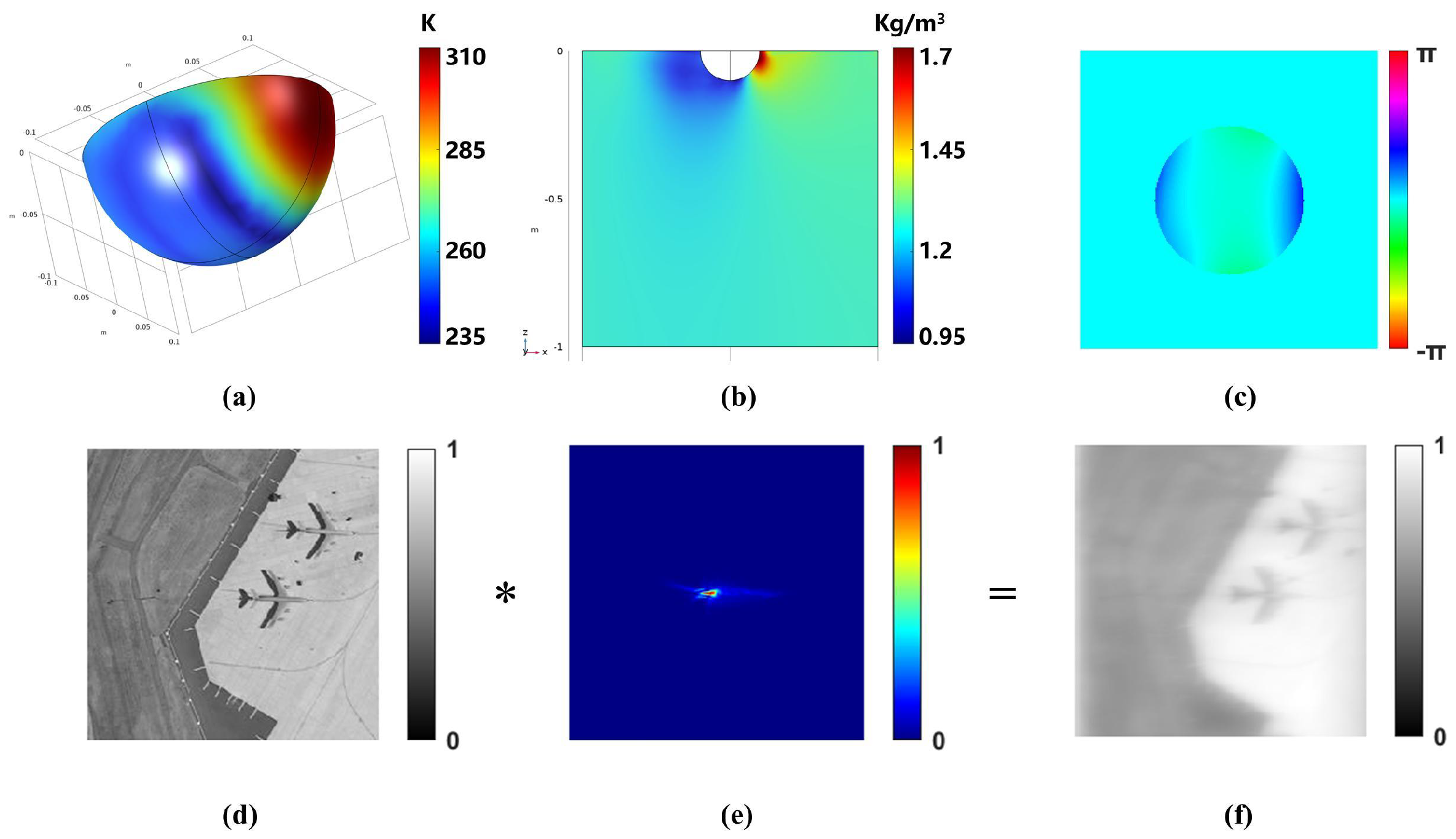
2.1. Degradation Model
2.2. Restoration Model
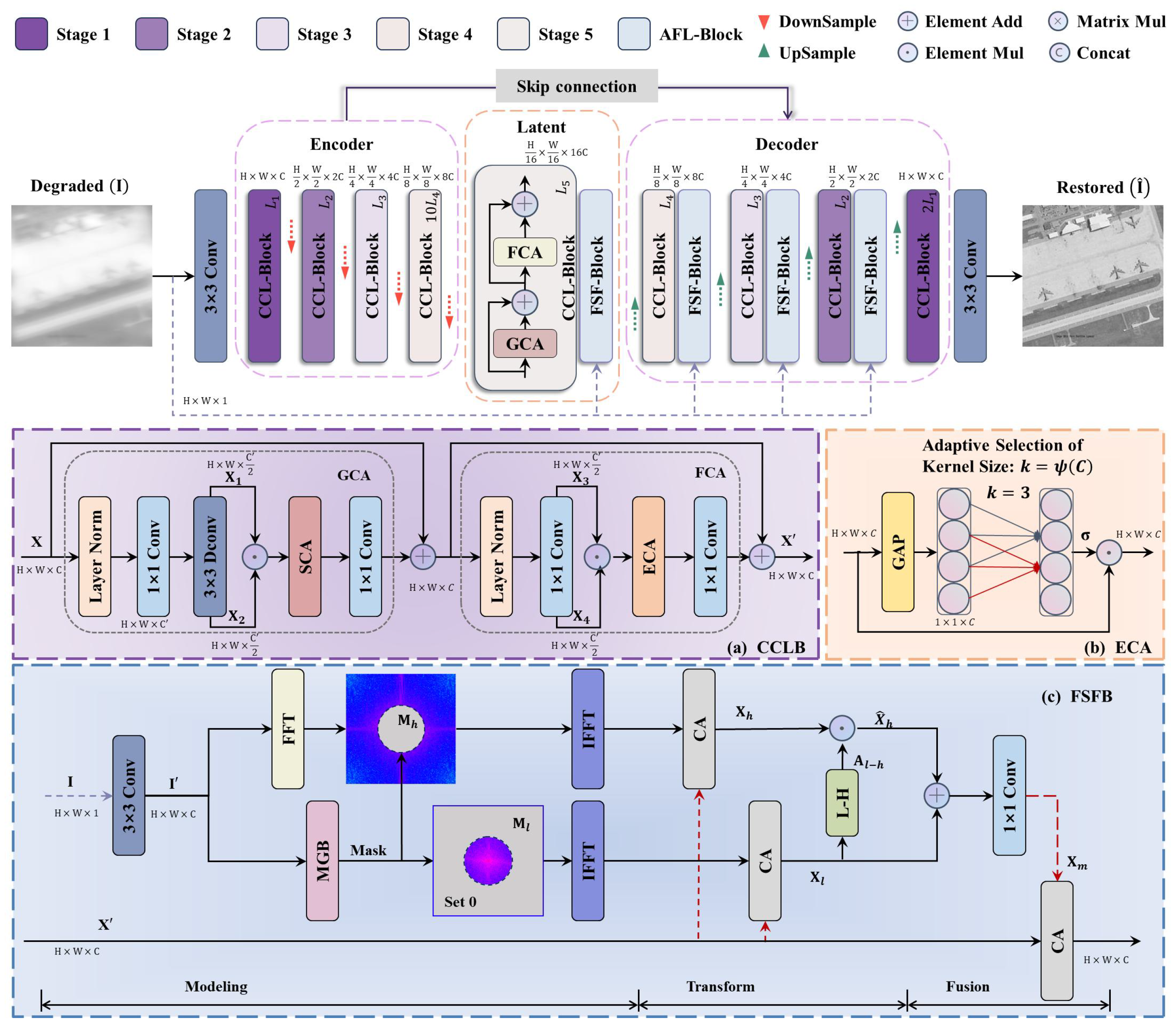
2.2.1. CCL-Block Introduction
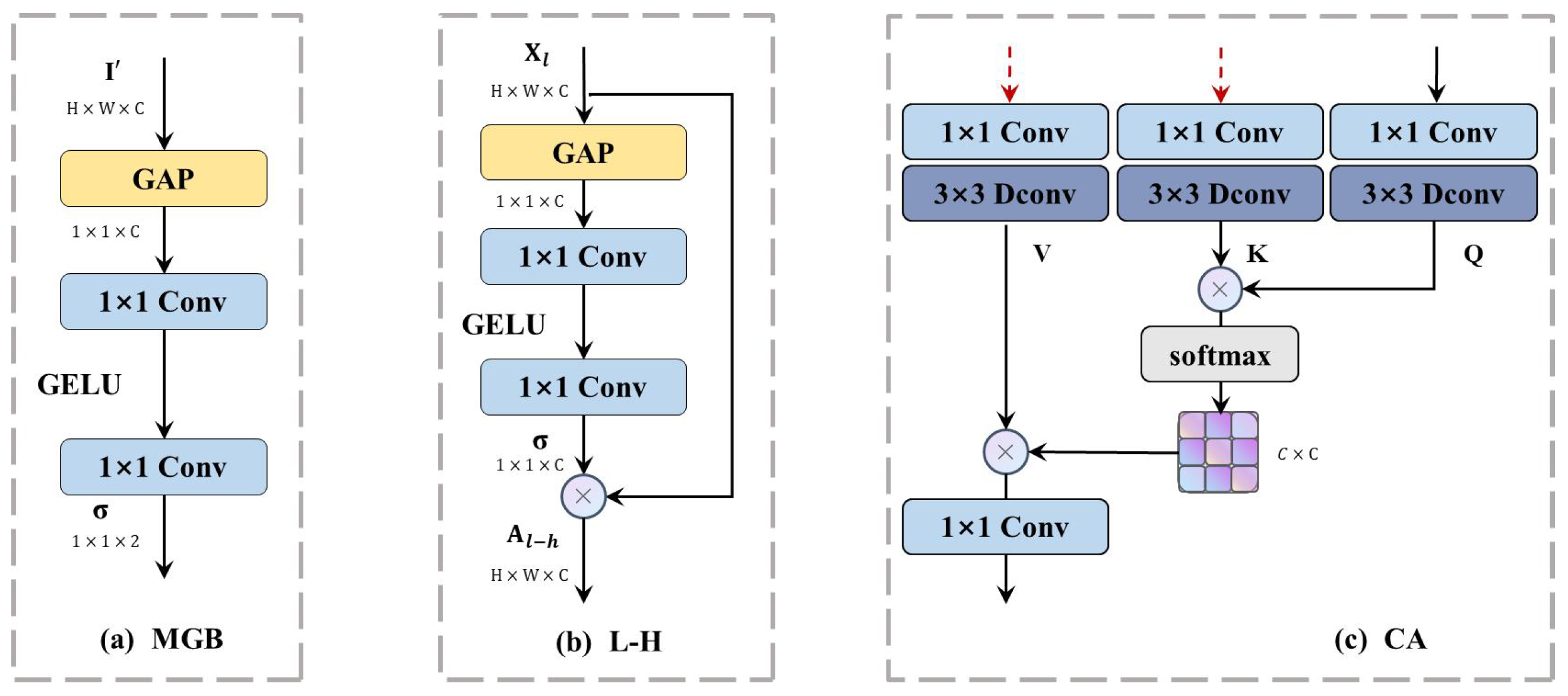
2.2.2. FSF-Block Introduction
3. Results
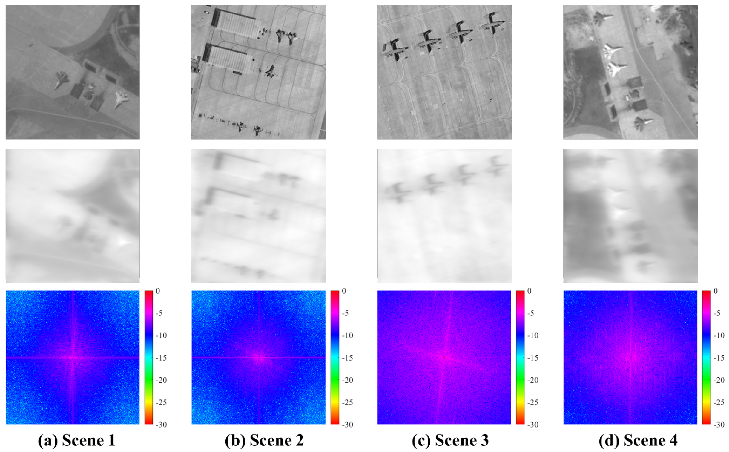
3.1. Image Datasets
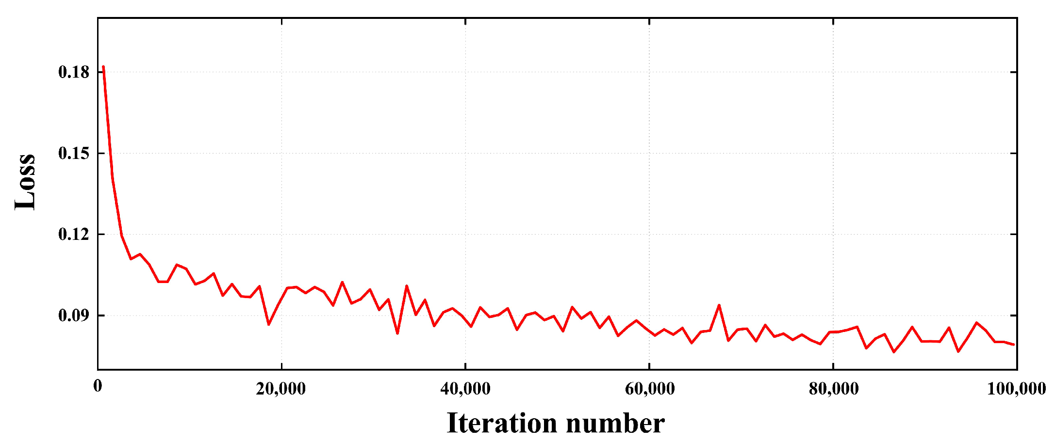
3.2. Loss Function
3.3. Implementation Details
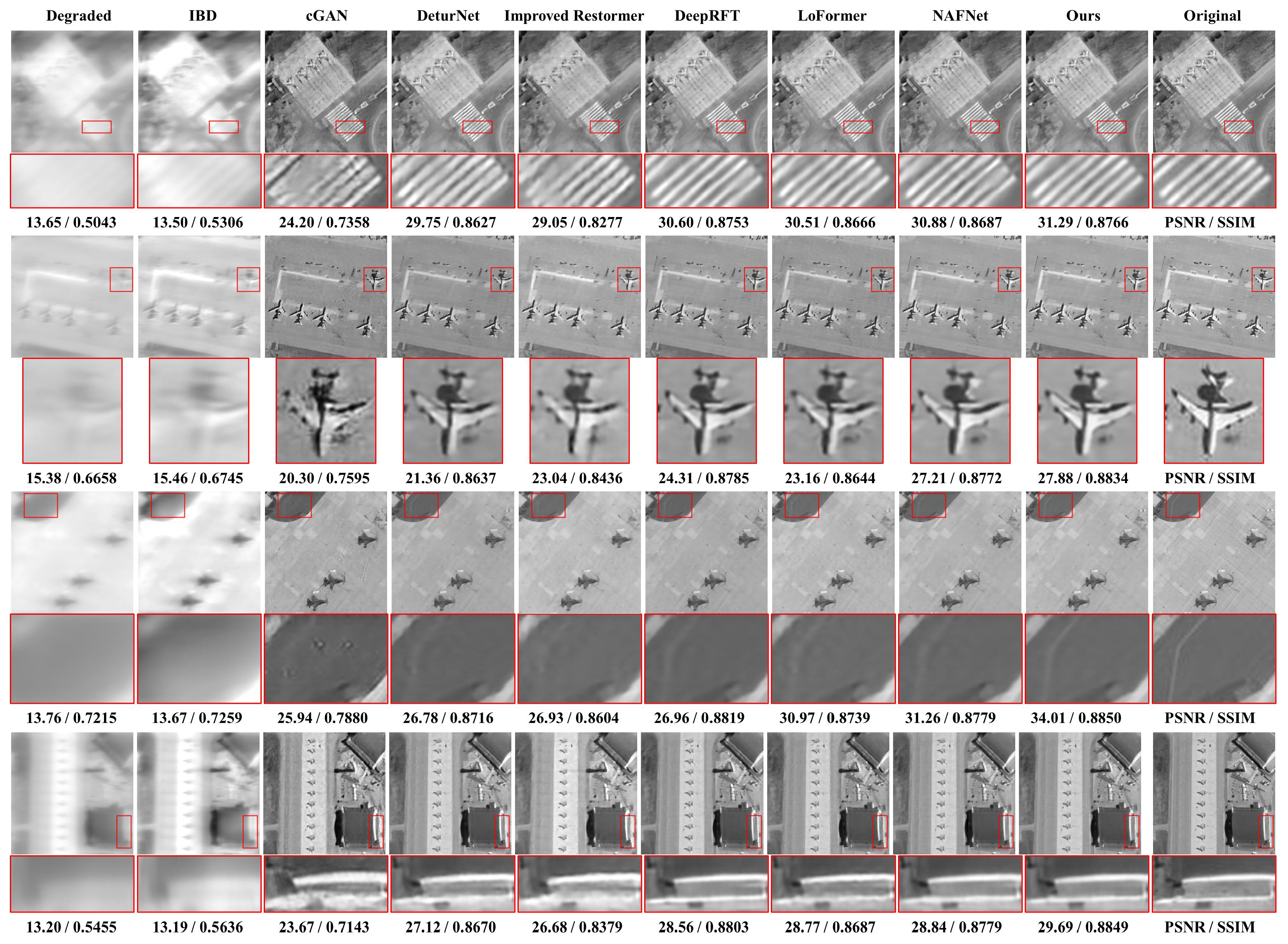
3.3.1. The Test of Image Restoration
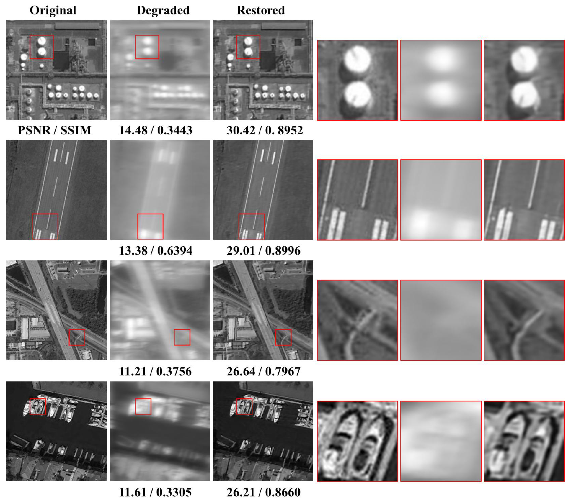
3.3.2. Scene Generalization Testing of AFS-NET
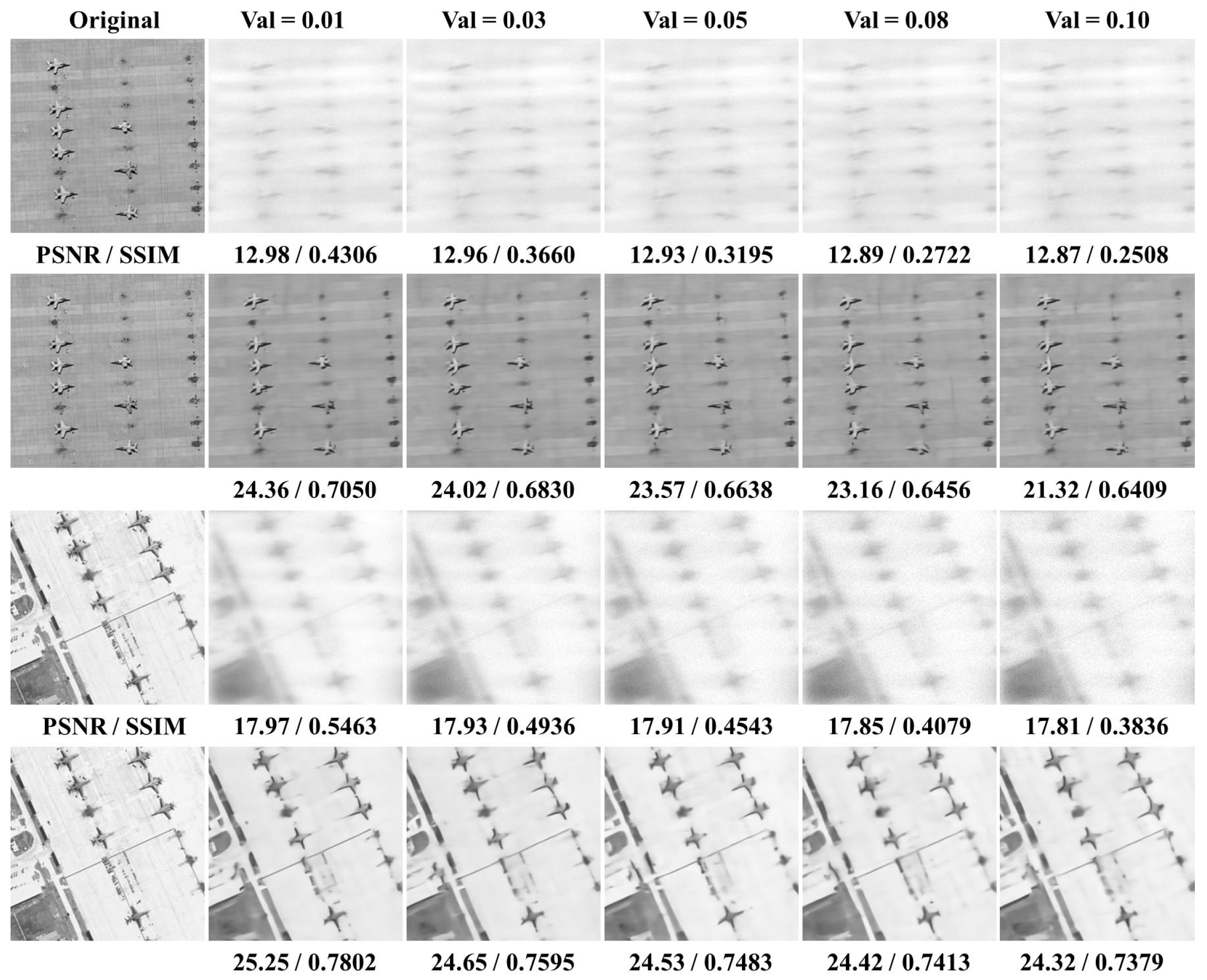
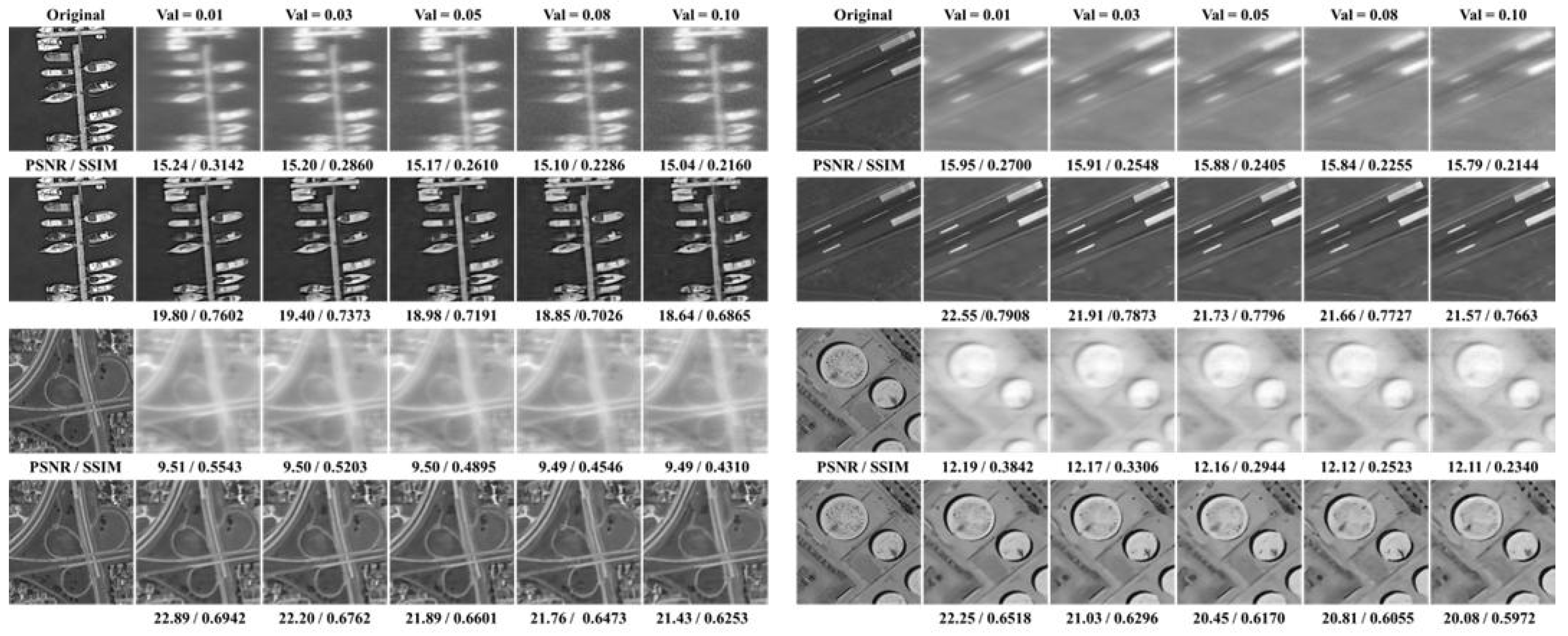
3.3.3. The Robustness of AFS-NET on Different Noises
3.3.4. Ablation Studies
4. Discussion
5. Conclusions
Author Contributions
Funding
Data Availability Statement
Conflicts of Interest
References
- Sutton, G.W.; Hwang, Y.F.; Pond, J.; Hwang, Y. Hypersonic interceptor aero-optics performance predictions. J. Spacecr. Rocket. 1994, 31, 592–599. [Google Scholar] [CrossRef]
- Yin, X.L. New subdiscipline of contemporary optics: Aero-optics. Eng. Sci. 2005, 7, 1–6. [Google Scholar]
- Zhang, T.X.; Hong, H.Y.; Zhang, X.Y. Aero-Optical Effect Correction: Principles, Methods and Applications; University of Science and Technology of China Press: Hefei, China, 2014. [Google Scholar]
- Zhang, L.Q.; Fei, J.D. Research on photoelectric correction method of aero-optical effect. Infrared Laser Eng. 2004, 6, 580–583. [Google Scholar]
- Richardson, W.H. Bayesian-based iterative method of image restoration. J. Opt. Soc. Am. 2013, 62, 55–59. [Google Scholar] [CrossRef]
- Ayers, G.R.; Dainty, J.C. Iterative blind deconvolution method and its applications. Opt. Lett. 1988, 13, 547–549. [Google Scholar] [CrossRef]
- Zhao, J.L.; Wang, Y. An accurate parameter estimation algorithm for fuzzy images based on quadratic Wiener filtering. Small Microcomput. Syst. 2014, 35, 1180–1183. [Google Scholar]
- Fish, D.A.; Brinicombe, A.M.; Pike, E.R.; Walker, J.G. Blind deconvolution by means of the Richardson–Lucy algorithm. J. Opt. Soc. Am. 1995, 12, 58–65. [Google Scholar] [CrossRef]
- Hong, H.; Shi, Y.; Zhang, T.; Liu, Z. A correction method for aero-optics thermal radiation effects based on gradient distribution and dark channel. Optoelectron. Lett. 2019, 15, 374–380. [Google Scholar] [CrossRef]
- Wang, Y.; Sui, X.; Wang, Y.; Liu, T.; Zhang, C.; Chen, Q. Contrast enhancement method in aero thermal radiation images based on cyclic multi-scale illumination self-similarity and gradient perception regularization. Opt. Express 2024, 32, 1650–1668. [Google Scholar] [CrossRef]
- You, Y.L.; Kaveh, M. A regularization approach to joint blur identification and image restoration. IEEE Trans. Image Process. 1996, 5, 416–428. [Google Scholar]
- Yuan, L.; Sun, J.; Quan, L.; Shum, H.-Y. Image deblurring with blurred/noisy image pairs. ACM Trans. Graph. 2007, 26, 1-es. [Google Scholar] [CrossRef]
- Su, Y.B.; Wang, Z.Y.; Liang, S.; Zhang, T.X. CGAN for simulation and digital image correction of aero transmission effect and aero heat radiation effect. In Proceedings of the Third International Conference on Photonics and Optical Engineering, Xi’an, China, 5–8 December 2018; Volume 11052, pp. 405–412. [Google Scholar]
- Gao, X.; Wang, S.; Cui, Y.; Wu, Z. Aero-optical image and video restoration based on mean filter and adversarial network. In Proceedings of the 2022 3rd International Conference on Computer Vision, Image and Deep Learning & International Conference on Computer Engineering and Applications (CVIDL & ICCEA), Changchun, China, 20–22 May 2022; pp. 528–532. [Google Scholar]
- Li, X.; Liu, X.; Wei, W.; Zhong, X.; Ma, H.; Chu, J. A deturnet-based method for recovering images degraded by atmospheric turbulence. Remote Sens. 2023, 15, 5071. [Google Scholar]
- Chen, L.; Chu, X.; Zhang, X.; Sun, J. Simple baselines for image restoration. In European Conference on Computer Vision; Springer Nature Switzerland: Cham, Switzerland, 2022; pp. 17–33. [Google Scholar]
- Cui, Y.; Zamir, S.W.; Khan, S.; Knoll, A.; Shah, M.; Khan, F.S. AdaIR: Adaptive All-in-One Image Restoration via Frequency Mining and Modulation. arXiv 2024, arXiv:2403.14614. [Google Scholar]
- Wang, Q.; Wu, B.; Zhu, P.; Li, P.; Zuo, W.; Hu, Q. ECA-Net: Efficient channel attention for deep convolutional neural networks. In Proceedings of the IEEE/CVF Conference on Computer Vision and Pattern Recognition, Seattle, WA, USA, 14–19 June 2020; pp. 11534–11542. [Google Scholar]
- Gladstone, J.H.; Dale, T.P. Researches on the Refraction, Dispersion, andSensitiveness of Liquids. Philos. Trans. R. Soc. Lond. 1862, 12, 448–453. [Google Scholar]
- Fender, J.S. Synthetic apertures: An overview. Synthetic Aperture Systems I. 1984, 440, 2–7. [Google Scholar]
- Meinel, B. Aperture synthesis using independent telescopes. Appl. Opt. 1970, 9, 2501. [Google Scholar] [CrossRef]
- Gardneretal, J.P. The James Webb Space Telescope. Space Sci. Rev. 2006, 123, 485–606. [Google Scholar]
- Hu, J.; Shen, L.; Sun, G. Squeeze-and-excitation networks. In Proceedings of the IEEE Conference on Computer Vision and Pattern Recognition, Salt Lake City, UT, USA, 18–22 June 2018; pp. 7132–7141. [Google Scholar]
- Zamir, S.W.; Arora, A.; Khan, S.; Hayat, M.; Khan, F.S.; Yang, M.H.; Shao, L.; bin Zayed, M. Multi-stage progressive image restoration. In Proceedings of the IEEE/CVF Conference on Computer Vision and Pattern Recognition, Nashville, TN, USA, 20–25 June 2021; pp. 14821–14831. [Google Scholar]
- Zamir, S.W.; Arora, A.; Khan, S.; Hayat, M.; Khan, F.S.; Yang, M.H. Restormer: Efficient transformer for high-resolution image restoration. In Proceedings of the IEEE/CVF Conference on Computer Vision and Pattern Recognition, New Orleans, LA, USA, 18–24 June 2022; pp. 5728–5739. [Google Scholar]
- Han, K.; Wang, Y.; Chen, H.; Chen, X.; Guo, J.; Liu, Z. A survey on vision transformer. IEEE Trans. Pattern Anal. Mach. Intell. 2022, 45, 87–110. [Google Scholar]
- Yu, W.Q.; Cheng, G.; Wang, M.J.; Yao, Y.; Xie, X.; Yao, X.; Han, J. MAR20: A Benchmark for Military Aircraft Recognition in Remote Sensing Images. Natl. Remote Sens. Bull. 2022, 27, 2688–2696. [Google Scholar]
- Wang, Q.; Gao, J.; Lin, W.; Li, X. NWPU-crowd: A large-scale benchmark for crowd counting and localization. IEEE Trans. Pattern Anal. Mach. Intell. 2020, 43, 2141–2149. [Google Scholar]
- Xia, G.S.; Hu, J.; Hu, F.; Shi, B.; Bai, X.; Zhing, T. AID: A benchmark data set for performance evalu-ation of aerial scene classification. IEEE Trans. Geosci. Remote Sens. 2017, 55, 3965–3981. [Google Scholar]
- Cho, S.-J.; Ji, S.-W.; Hong, J.-P.; Jung, S.-W.; Ko, S.-J. Rethinking coarse-to-fine approach in single image deblurring. In Proceedings of the IEEE/CVF International Conference on Computer Vision, Montreal, BC, Canada, 11–17 October 2021; pp. 4641–4650. [Google Scholar]
- Mao, X.; Liu, Y.; Liu, F.; Li, Q.; Shen, W.; Wang, Y. Intriguing findings of frequency selection for image deblurring. Proc. AAAI Conf. Artif. Intell. 2023, 37, 1905–1913. [Google Scholar]
- Jiang, K.; Wang, Z.; Yi, P.; Chen, C.; Huang, B.; Luo, Y.; Ma, J.; Jiang, J. Multi-scale progressive fusion network for single image deraining. In Proceedings of the IEEE/CVF Conference on Computer Vision and Pattern Recognition, Seattle, WA, USA, 13–19 June 2020; pp. 8346–8355. [Google Scholar]
- Akmaral, A.; Zafar, M.H. Efficient Transformer for High Resolution Image Motion Deblurring. arXiv 2025, arXiv:2501.18403. [Google Scholar]
- Mao, X.; Wang, J.; Xie, X.; Li, Q.; Wang, Y. Loformer: Local frequency transformer for image deblur-ring. In Proceedings of the 32nd ACM International Conference on Multimedia, Melbourne, VIC, Australia, 28 October–1 November 2024; pp. 10382–10391. [Google Scholar]


| PSNR | SSIM | MACs (G) | Times (s) | |
|---|---|---|---|---|
| Degraded | 13.66 | 0.5317 | - | - |
| IBD | 13.68 | 0.5448 | - | 15.05 |
| CGAN | 22.82 | 0.6951 | 78.30 | 0.077 |
| DeturNET | 25.14 | 0.8348 | 88.70 | 0.033 |
| Improved Restormer | 25.88 | 0.8033 | 64.46 | 0.097 |
| DEEPRFT | 26.22 | 0.8488 | 63.46 | 0.089 |
| LoFormer-B | 26.32 | 0.8375 | 73.04 | 0.132 |
| NAFNET-64 | 26.62 | 0.8423 | 63.21 | 0.044 |
| Ours | 27.42 | 0.8504 | 50.16 | 0.026 |
| Scene Test | Restoration | ||||
|---|---|---|---|---|---|
| Sets | PSNR | SSIM | PSNR | SSIM | |
| NWPU | Storage | 13.90 | 0.3526 | 24.81 | 0.8096 |
| Runway | 12.22 | 0.5710 | 24.52 | 0.8549 | |
| Overpass | 10.27 | 0.3305 | 23.56 | 0.7938 | |
| Harbor | 11.51 | 0.3615 | 23.51 | 0.8106 | |
| AID | Playground | 12.74 | 0.4767 | 25.70 | 0.8272 |
| School | 12.10 | 0.2650 | 24.47 | 0.7997 | |
| Square | 12.72 | 0.3280 | 24.10 | 0.7986 | |
| Center | 15.08 | 0.3724 | 24.07 | 0.7866 | |
| Church | 12.00 | 0.2608 | 23.68 | 0.7618 | |
| Stadium | 14.77 | 0.3933 | 23.53 | 0.8050 | |
| Noise Test | Restoration | ||||
|---|---|---|---|---|---|
| PSNR | SSIM | PSNR | SSIM | ||
| MAR20 | Var = 0.01 | 13.65 | 0.4804 | 24.13 | 0.7200 |
| Var = 0.03 | 13.61 | 0.4144 | 24.04 | 0.7003 | |
| Var = 0.05 | 13.58 | 0.3707 | 23.83 | 0.6880 | |
| Var = 0.08 | 13.53 | 0.3254 | 23.54 | 0.6746 | |
| Var = 0.10 | 13.50 | 0.3027 | 23.37 | 0.6665 | |
| PSNR | SSIM | PSNR | SSIM | ||
| NWPU | Var = 0.01 | 11.96 | 0.3650 | 20.97 | 0.6604 |
| Var = 0.03 | 11.93 | 0.3135 | 20.64 | 0.6388 | |
| Var = 0.05 | 11.90 | 0.2790 | 20.40 | 0.6243 | |
| Var = 0.08 | 11.85 | 0.2428 | 20.14 | 0.6078 | |
| Var = 0.10 | 11.82 | 0.2248 | 20.02 | 0.5988 | |
| Net | L-H | Rect Mask | Ellip Mask | PSNR | SSIM |
|---|---|---|---|---|---|
| a | ✔ | ✔ | 27.19 | 0.8493 | |
| b | ✔ | 27.31 | 0.8487 | ||
| c | ✔ | ✔ | 27.42 | 0.8504 |
| Net | ECA | FSF-Block | PSNR | SSIM | Parms (M) | FLOPs (G) |
|---|---|---|---|---|---|---|
| a | 26.85 | 0.8495 | 34.50 | 35.69 | ||
| b | ✔ | 26.99 | 0.8556 | 34.50 | 35.74 | |
| c | ✔ | 27.25 | 0.8466 | 53.80 | 50.11 | |
| d | ✔ | ✔ | 27.42 | 0.8504 | 53.80 | 50.16 |
| Loss Method | PSNR | SSIM |
|---|---|---|
| 26.42 | 0.8308 | |
| 27.24 | 0.8493 | |
| 27.32 | 0.8494 | |
| 27.42 | 0.8504 |
Disclaimer/Publisher’s Note: The statements, opinions and data contained in all publications are solely those of the individual author(s) and contributor(s) and not of MDPI and/or the editor(s). MDPI and/or the editor(s) disclaim responsibility for any injury to people or property resulting from any ideas, methods, instructions or products referred to in the content. |
© 2025 by the authors. Licensee MDPI, Basel, Switzerland. This article is an open access article distributed under the terms and conditions of the Creative Commons Attribution (CC BY) license (https://creativecommons.org/licenses/by/4.0/).
Share and Cite
Huang, Y.; Zhang, Q.; Ma, X.; Ma, H. Efficient Aero-Optical Degraded Image Restoration via Adaptive Frequency Selection. Remote Sens. 2025, 17, 1122. https://doi.org/10.3390/rs17071122
Huang Y, Zhang Q, Ma X, Ma H. Efficient Aero-Optical Degraded Image Restoration via Adaptive Frequency Selection. Remote Sensing. 2025; 17(7):1122. https://doi.org/10.3390/rs17071122
Chicago/Turabian StyleHuang, Yingjiao, Qingpeng Zhang, Xiafei Ma, and Haotong Ma. 2025. "Efficient Aero-Optical Degraded Image Restoration via Adaptive Frequency Selection" Remote Sensing 17, no. 7: 1122. https://doi.org/10.3390/rs17071122
APA StyleHuang, Y., Zhang, Q., Ma, X., & Ma, H. (2025). Efficient Aero-Optical Degraded Image Restoration via Adaptive Frequency Selection. Remote Sensing, 17(7), 1122. https://doi.org/10.3390/rs17071122