


Detecting Long-Term Spatiotemporal Dynamics of Urban Green Spaces with Training Sample Migration Method

 , and
, and 
Abstract
:1. Introduction
2. Materials and Methods
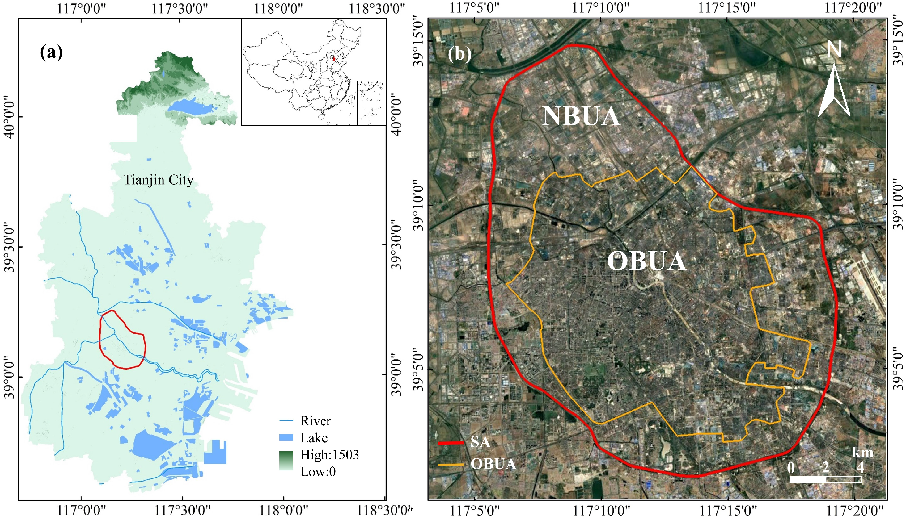
2.1. Study Area
2.2. Dataset
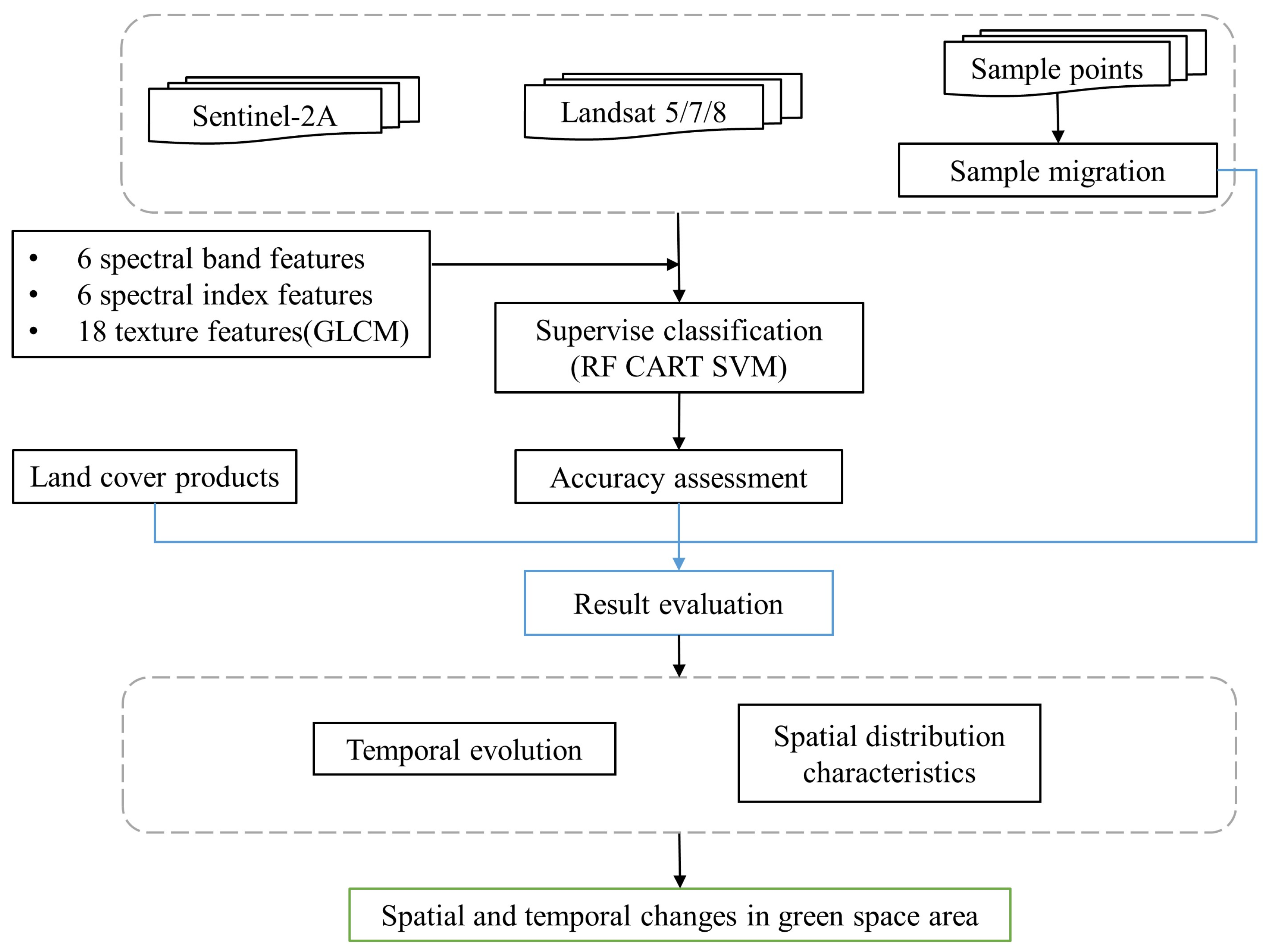
2.3. Methods
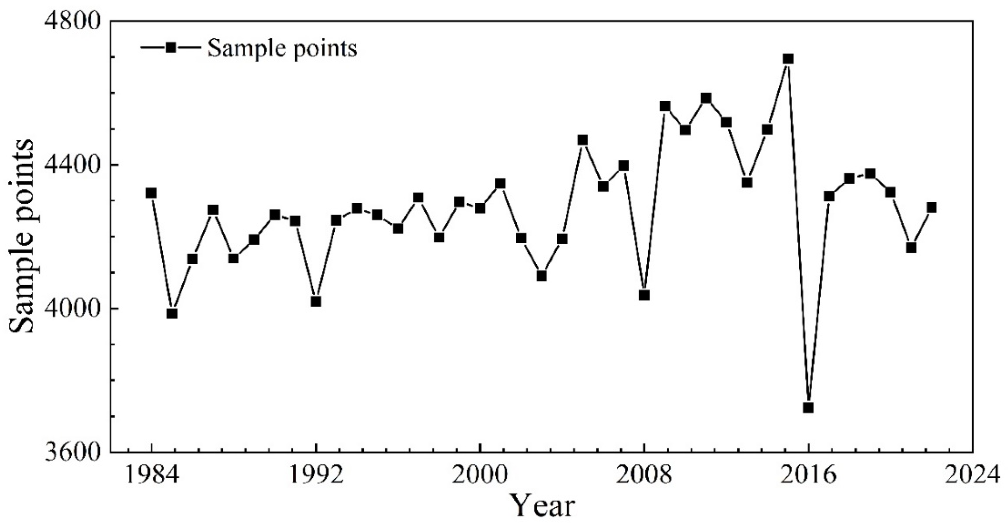
2.3.1. Training Sample Migration
2.3.2. Supervised Classification
2.3.3. Accuracy Assessment
2.3.4. Landscape Pattern Index
3. Results
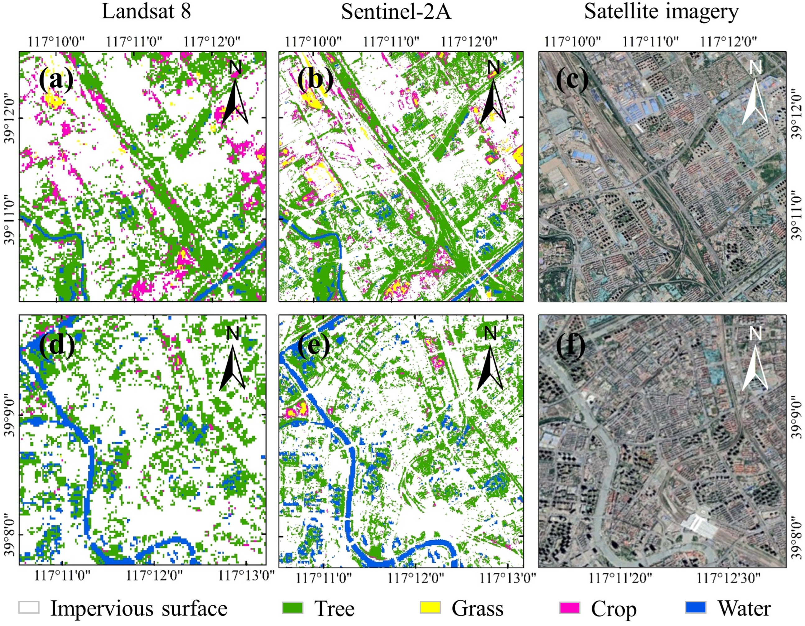
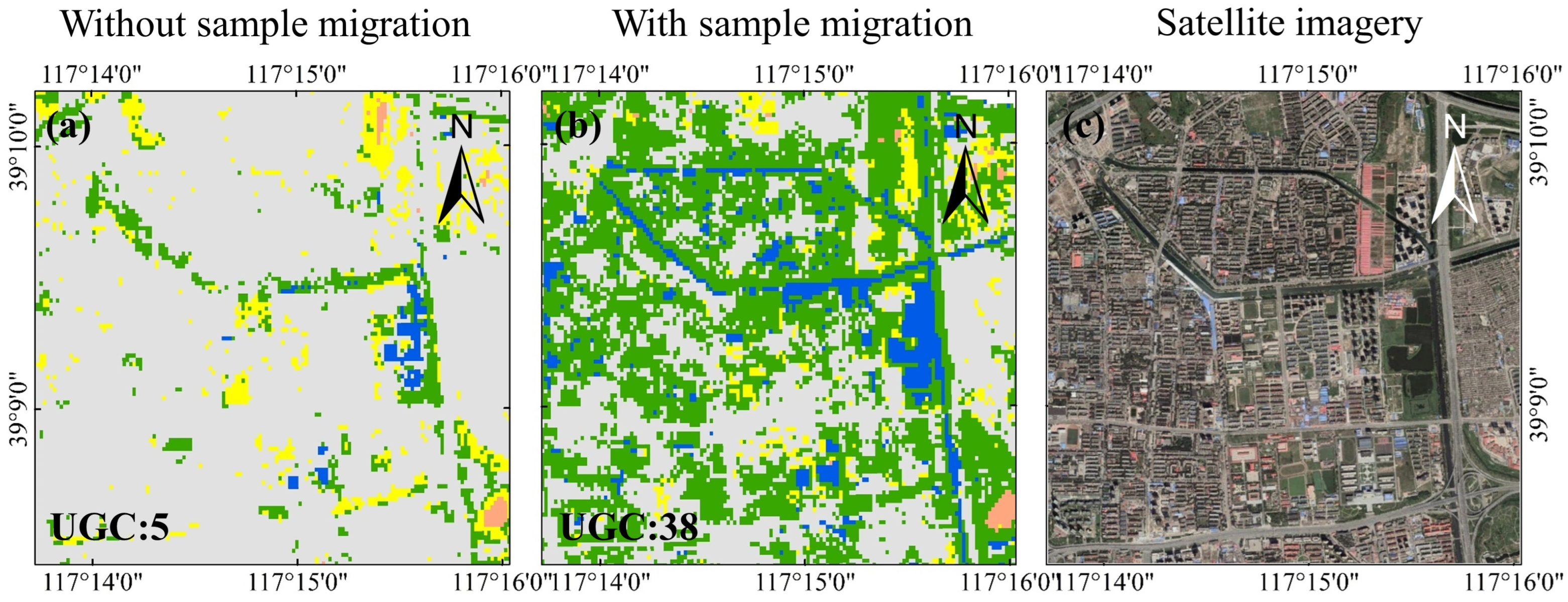
3.1. Mapping UGSs with Training Sample Migration
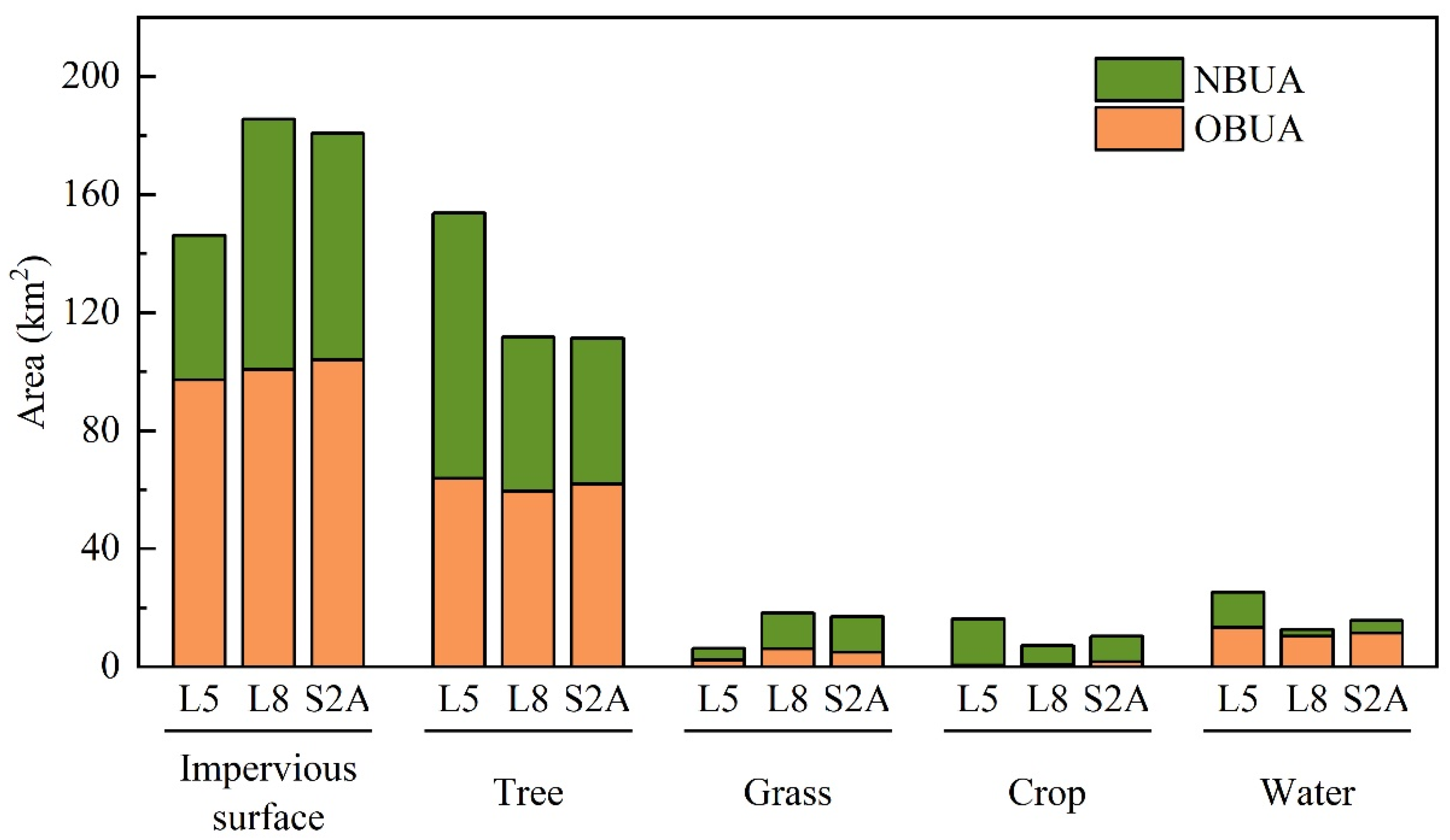
3.2. Spatial Distribution of UGSs
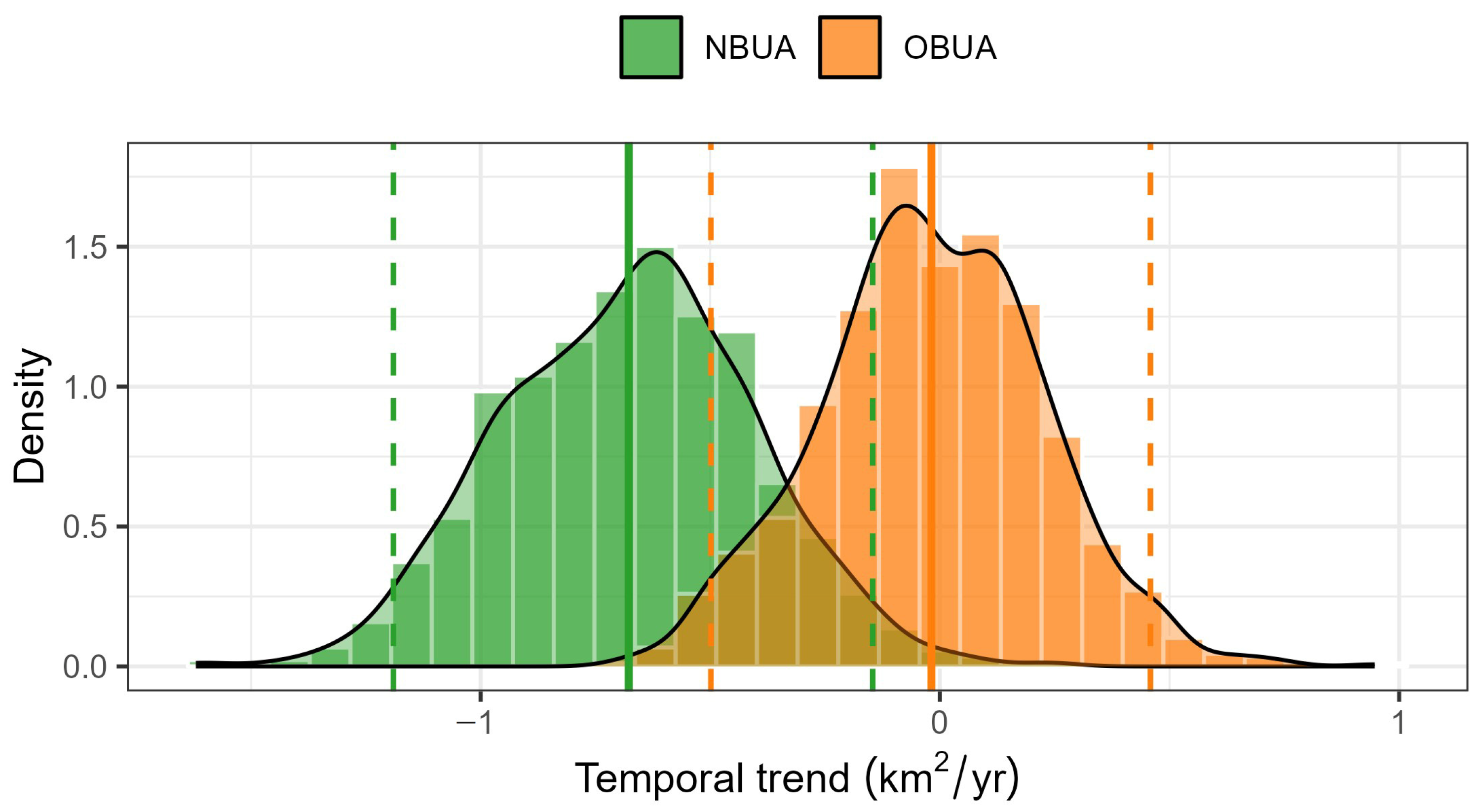
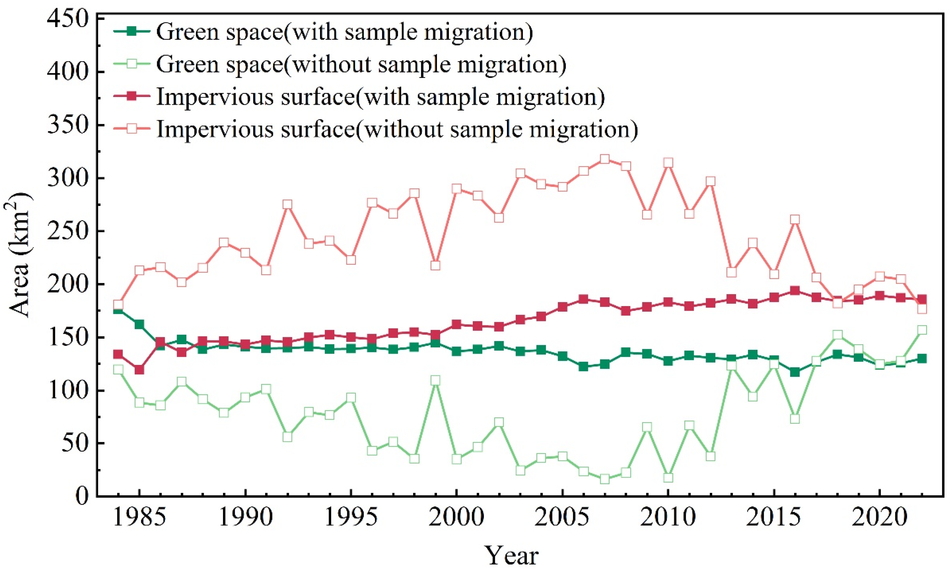
3.3. Temporal Trend of UGS
4. Discussion
4.1. Reliability of Long-Term Annual Maps of UGSs with Sample Migration Method
4.2. Long-Term Spatiotemporal Dynamics of UGS
4.3. Implications for Global and Local UGSs-Related Research
4.4. Limitations
5. Conclusions
Author Contributions
Funding
Data Availability Statement
Acknowledgments
Conflicts of Interest
Appendix A

| Year | UA | PA | OA | Kappa | ||||||||
|---|---|---|---|---|---|---|---|---|---|---|---|---|
| Impervious Surface | Tree | Grass | Crop | Water | Impervious Surface | Tree | Grass | Crop | Water | |||
| 1984 | 0.67 | 0.65 | 0.46 | 0.81 | 0.78 | 0.69 | 0.74 | 0.30 | 0.83 | 0.62 | 0.70 | 0.66 |
| 1985 | 0.72 | 0.63 | 0.39 | 0.64 | 0.93 | 0.60 | 0.78 | 0.25 | 0.81 | 0.61 | 0.67 | 0.52 |
| 1986 | 0.68 | 0.60 | 0.52 | 0.80 | 0.88 | 0.70 | 0.71 | 0.25 | 0.84 | 0.67 | 0.68 | 0.54 |
| 1987 | 0.72 | 0.62 | 0.34 | 0.76 | 0.91 | 0.72 | 0.76 | 0.22 | 0.88 | 0.59 | 0.71 | 0.57 |
| 1988 | 0.67 | 0.64 | 0.58 | 0.79 | 0.80 | 0.72 | 0.73 | 0.22 | 0.90 | 0.74 | 0.70 | 0.56 |
| 1989 | 0.73 | 0.66 | 0.45 | 0.84 | 0.83 | 0.80 | 0.73 | 0.25 | 0.89 | 0.67 | 0.72 | 0.61 |
| 1990 | 0.78 | 0.62 | 0.40 | 0.80 | 0.86 | 0.72 | 0.80 | 0.22 | 0.85 | 0.74 | 0.72 | 0.61 |
| 1991 | 0.68 | 0.67 | 0.54 | 0.85 | 0.76 | 0.70 | 0.76 | 0.31 | 0.87 | 0.72 | 0.71 | 0.58 |
| 1992 | 0.69 | 0.69 | 0.41 | 0.83 | 0.79 | 0.73 | 0.77 | 0.23 | 0.86 | 0.77 | 0.72 | 0.60 |
| 1993 | 0.76 | 0.67 | 0.56 | 0.83 | 0.88 | 0.76 | 0.81 | 0.26 | 0.85 | 0.66 | 0.74 | 0.61 |
| 1994 | 0.74 | 0.62 | 0.80 | 0.83 | 0.78 | 0.76 | 0.75 | 0.25 | 0.87 | 0.60 | 0.70 | 0.57 |
| 1995 | 0.79 | 0.67 | 0.53 | 0.76 | 0.84 | 0.78 | 0.77 | 0.23 | 0.86 | 0.82 | 0.74 | 0.62 |
| 1996 | 0.77 | 0.63 | 0.45 | 0.83 | 0.81 | 0.78 | 0.76 | 0.23 | 0.82 | 0.74 | 0.72 | 0.59 |
| 1997 | 0.78 | 0.70 | 0.65 | 0.80 | 0.86 | 0.78 | 0.82 | 0.25 | 0.91 | 0.79 | 0.75 | 0.63 |
| 1998 | 0.77 | 0.68 | 0.34 | 0.84 | 0.81 | 0.81 | 0.77 | 0.22 | 0.89 | 0.79 | 0.74 | 0.63 |
| 1999 | 0.77 | 0.65 | 0.45 | 0.92 | 0.83 | 0.79 | 0.79 | 0.21 | 0.89 | 0.73 | 0.75 | 0.64 |
| 2000 | 0.71 | 0.67 | 0.39 | 0.90 | 0.84 | 0.83 | 0.73 | 0.22 | 0.90 | 0.68 | 0.73 | 0.62 |
| 2001 | 0.78 | 0.70 | 0.66 | 0.88 | 0.83 | 0.83 | 0.82 | 0.24 | 0.91 | 0.67 | 0.76 | 0.65 |
| 2002 | 0.71 | 0.63 | 0.39 | 0.83 | 0.80 | 0.72 | 0.75 | 0.22 | 0.83 | 0.72 | 0.70 | 0.57 |
| 2003 | 0.69 | 0.65 | 0.63 | 0.94 | 0.85 | 0.78 | 0.77 | 0.22 | 0.86 | 0.73 | 0.73 | 0.61 |
| 2004 | 0.73 | 0.68 | 0.53 | 0.93 | 0.89 | 0.82 | 0.80 | 0.22 | 0.88 | 0.73 | 0.75 | 0.63 |
| 2005 | 0.73 | 0.66 | 0.53 | 0.98 | 0.85 | 0.86 | 0.78 | 0.21 | 0.88 | 0.77 | 0.74 | 0.63 |
| 2006 | 0.72 | 0.72 | 0.45 | 0.92 | 0.79 | 0.89 | 0.72 | 0.23 | 0.90 | 0.76 | 0.75 | 0.64 |
| 2007 | 0.72 | 0.75 | 0.70 | 0.87 | 0.78 | 0.88 | 0.80 | 0.21 | 0.85 | 0.76 | 0.75 | 0.64 |
| 2008 | 0.80 | 0.67 | 0.28 | 0.90 | 0.92 | 0.82 | 0.86 | 0.21 | 0.90 | 0.80 | 0.76 | 0.65 |
| 2009 | 0.77 | 0.74 | 0.65 | 0.97 | 0.80 | 0.89 | 0.85 | 0.25 | 0.91 | 0.79 | 0.79 | 0.69 |
| 2010 | 0.77 | 0.75 | 0.57 | 0.88 | 0.83 | 0.89 | 0.83 | 0.23 | 0.91 | 0.82 | 0.78 | 0.68 |
| 2011 | 0.78 | 0.72 | 0.49 | 0.90 | 0.82 | 0.84 | 0.87 | 0.23 | 0.85 | 0.81 | 0.77 | 0.66 |
| 2012 | 0.79 | 0.74 | 0.40 | 0.87 | 0.84 | 0.81 | 0.87 | 0.24 | 0.90 | 0.70 | 0.76 | 0.65 |
| 2013 | 0.81 | 0.78 | 0.65 | 0.99 | 0.78 | 0.93 | 0.91 | 0.26 | 0.90 | 0.75 | 0.80 | 0.71 |
| 2014 | 0.84 | 0.76 | 0.58 | 0.97 | 0.85 | 0.88 | 0.90 | 0.28 | 0.93 | 0.79 | 0.81 | 0.72 |
| 2015 | 0.85 | 0.78 | 0.55 | 0.92 | 0.85 | 0.88 | 0.90 | 0.30 | 0.90 | 0.80 | 0.81 | 0.72 |
| 2016 | 0.85 | 0.78 | 0.55 | 0.94 | 0.80 | 0.90 | 0.87 | 0.24 | 0.91 | 0.81 | 0.81 | 0.71 |
| 2017 | 0.85 | 0.78 | 0.62 | 0.93 | 0.92 | 0.89 | 0.92 | 0.32 | 0.91 | 0.80 | 0.82 | 0.73 |
| 2018 | 0.84 | 0.79 | 0.70 | 0.94 | 0.84 | 0.91 | 0.88 | 0.41 | 0.90 | 0.74 | 0.82 | 0.73 |
| 2019 | 0.84 | 0.79 | 0.59 | 0.93 | 0.87 | 0.87 | 0.93 | 0.32 | 0.88 | 0.84 | 0.81 | 0.72 |
| 2020 | 0.88 | 0.78 | 0.68 | 0.85 | 0.85 | 0.91 | 0.91 | 0.38 | 0.82 | 0.75 | 0.82 | 0.73 |
| 2021 | 0.83 | 0.75 | 0.76 | 0.93 | 0.86 | 0.88 | 0.88 | 0.36 | 0.85 | 0.73 | 0.80 | 0.70 |
| 2022 | 0.83 | 0.77 | 0.58 | 0.94 | 0.78 | 0.86 | 0.90 | 0.31 | 0.83 | 0.78 | 0.79 | 0.69 |
References
- World Health Organization. Urban Green Spaces: A Brief for Action; World Health Organization: Geneva, Switzerland, 2017; Available online: https://www.who.int/europe/publications/i/item/9789289052498 (accessed on 13 April 2025).
- Li, P.; Wang, Z.-H.; Wang, C. The Potential of Urban Irrigation for Counteracting Carbon-Climate Feedback. Nat. Commun. 2024, 15, 2437. [Google Scholar] [CrossRef] [PubMed]
- Lian, X.; Jiao, L.; Liu, Z.; Jia, Q.; Liu, W.; Liu, Y. A Detection of Street Trees and Green Space: Understanding Contribution of Urban Trees to Climate Change Mitigation. Urban For. Urban Green. 2024, 102, 128561. [Google Scholar] [CrossRef]
- Tang, L.; Shao, G.; Groffman, P.M. Urban Trees: How to Maximize Their Benefits for Humans and the Environment. Nature 2024, 626, 261. [Google Scholar] [CrossRef]
- Chen, W.Y. The Role of Urban Green Infrastructure in Offsetting Carbon Emissions in 35 Major Chinese Cities: A Nationwide Estimate. Cities 2015, 44, 112–120. [Google Scholar] [CrossRef]
- Sun, Y.; Xie, S.; Zhao, S. Valuing Urban Green Spaces in Mitigating Climate Change: A City-Wide Estimate of Aboveground Carbon Stored in Urban Green Spaces of China’s Capital. Glob. Change Biol. 2019, 25, 1717–1732. [Google Scholar] [CrossRef]
- Schwaab, J.; Meier, R.; Mussetti, G.; Seneviratne, S.; Bürgi, C.; Davin, E.L. The Role of Urban Trees in Reducing Land Surface Temperatures in European Cities. Nat. Commun. 2021, 12, 6763. [Google Scholar] [CrossRef]
- Venter, Z.S.; Hassani, A.; Stange, E.; Schneider, P.; Castell, N. Reassessing the Role of Urban Green Space in Air Pollution Control. Proc. Natl. Acad. Sci. USA 2024, 121, e2306200121. [Google Scholar] [CrossRef]
- Wolch, J.R.; Byrne, J.; Newell, J.P. Urban Green Space, Public Health, and Environmental Justice: The Challenge of Making Cities “Just Green Enough”. Landsc. Urban Plan. 2014, 125, 234–244. [Google Scholar] [CrossRef]
- Bakhtsiyarava, M.; Moran, M.; Ju, Y.; Zhou, Y.; Rodriguez, D.A.; Dronova, I.; de Fatima Rodrigues Pereira de Pina, M.; de Matos, V.P.; Skaba, D.A. Potential Drivers of Urban Green Space Availability in Latin American Cities. Nat. Cities 2024, 1, 842–852. [Google Scholar] [CrossRef]
- Leng, S.; Sun, R.; Yang, X.; Chen, L. Global Inequities in Population Exposure to Urban Greenspaces Increased amidst Tree and Nontree Vegetation Cover Expansion. Commun. Earth Env. 2023, 4, 464. [Google Scholar] [CrossRef]
- Sun, J.; Wang, X.; Chen, A.; Ma, Y.; Cui, M.; Piao, S. NDVI Indicated Characteristics of Vegetation Cover Change in China’s Metropolises over the Last Three Decades. Environ. Monit. Assess. 2011, 179, 1–14. [Google Scholar] [CrossRef] [PubMed]
- Zhang, X.; Brandt, M.; Tong, X.; Tong, X.; Zhang, W.; Fensholt, R. Urban Core Greening Balances Browning in Urban Expansion Areas in China during Recent Decades. J. Remote Sens. 2024, 4, 0112. [Google Scholar] [CrossRef]
- Feng, F.; Yang, X.; Jia, B.; Li, X.; Li, X.; Xu, C.; Wang, K. Variability of Urban Fractional Vegetation Cover and Its Driving Factors in 328 Cities in China. Sci. China Earth Sci. 2024, 67, 466–482. [Google Scholar] [CrossRef]
- Liu, X.; Wang, S.; Wu, P.; Feng, K.; Hubacek, K.; Li, X.; Sun, L. Impacts of Urban Expansion on Terrestrial Carbon Storage in China. Environ. Sci. Technol. 2019, 53, 6834–6844. [Google Scholar] [CrossRef]
- Huang, C.; Yang, J.; Clinton, N.; Yu, L.; Huang, H.; Dronova, I.; Jin, J. Mapping the Maximum Extents of Urban Green Spaces in 1039 Cities Using Dense Satellite Images. Environ. Res. Lett. 2021, 16, 064072. [Google Scholar] [CrossRef]
- Qian, Y.; Zhou, W.; Yu, W.; Pickett, S.T.A. Quantifying Spatiotemporal Pattern of Urban Greenspace: New Insights from High Resolution Data. Landsc. Ecol. 2015, 30, 1165–1173. [Google Scholar] [CrossRef]
- Yang, J.; Huang, C.; Zhang, Z.; Wang, L. The Temporal Trend of Urban Green Coverage in Major Chinese Cities between 1990 and 2010. Urban For. Urban Green. 2014, 13, 19–27. [Google Scholar] [CrossRef]
- Kuang, W.; Zhang, S.; Li, X.; Lu, D. A 30 m Resolution Dataset of China’s Urban Impervious Surface Area and Green Space, 2000–2018. Earth Syst. Sci. Data 2021, 13, 63–82. [Google Scholar] [CrossRef]
- Liu, X.; Hu, G.; Chen, Y.; Li, X.; Xu, X.; Li, S.; Pei, F.; Wang, S. High-Resolution Multi-Temporal Mapping of Global Urban Land Using Landsat Images Based on the Google Earth Engine Platform. Remote Sens. Environ. 2018, 209, 227–239. [Google Scholar] [CrossRef]
- Li, X.; Gong, P.; Liang, L. A 30-Year (1984–2013) Record of Annual Urban Dynamics of Beijing City Derived from Landsat Data. Remote Sens. Environ. 2015, 166, 78–90. [Google Scholar] [CrossRef]
- Sexton, J.O.; Huang, C.; Channan, S.; Baker, M.E.; Townshend, J.R. Urban Growth of the Washington, D.C.–Baltimore, MD Metropolitan Region from 1984 to 2010 by Annual, Landsat-Based Estimates of Impervious Cover. Remote Sens. Environ. 2013, 129, 42–53. [Google Scholar] [CrossRef]
- Zhu, Z.; Zhou, Y.; Seto, K.C.; Stokes, E.C.; Deng, C.; Pickett, S.T.A.; Taubenböck, H. Understanding an Urbanizing Planet: Strategic Directions for Remote Sensing. Remote Sens. Environ. 2019, 228, 164–182. [Google Scholar] [CrossRef]
- Kopecká, M.; Szatmári, D.; Rosina, K. Analysis of Urban Green Spaces Based on Sentinel-2A: Case Studies from Slovakia. Land 2017, 6, 25. [Google Scholar] [CrossRef]
- Masό, J.; Zabala, A.; Pons, X. Protected Areas from Space Map Browser with Fast Visualization and Analytical Operations on the Fly. Characterizing Statistical Uncertainties and Balancing Them with Visual Perception. ISPRS Int. J. Geo-Inf. 2020, 9, 300. [Google Scholar] [CrossRef]
- Huang, H.; Wang, J.; Liu, C.; Liang, L.; Li, C.; Gong, P. The Migration of Training Samples towards Dynamic Global Land Cover Mapping. ISPRS J. Photogramm. Remote Sens. 2020, 161, 27–36. [Google Scholar] [CrossRef]
- Li, C.; Gong, P.; Wang, J.; Zhu, Z.; Biging, G.S.; Yuan, C.; Hu, T.; Zhang, H.; Wang, Q.; Li, X.; et al. The First All-Season Sample Set for Mapping Global Land Cover with Landsat-8 Data. Sci. Bull. 2017, 62, 508–515. [Google Scholar] [CrossRef]
- Duro, D.C.; Franklin, S.E.; Dubé, M.G. A Comparison of Pixel-Based and Object-Based Image Analysis with Selected Machine Learning Algorithms for the Classification of Agricultural Landscapes Using SPOT-5 HRG Imagery. Remote Sens. Environ. 2012, 118, 259–272. [Google Scholar] [CrossRef]
- Qian, Y.; Zhou, W.; Yan, J.; Li, W.; Han, L. Comparing Machine Learning Classifiers for Object-Based Land Cover Classification Using Very High Resolution Imagery. Remote Sens. 2014, 7, 153–168. [Google Scholar] [CrossRef]
- Wieland, M.; Pittore, M. Performance Evaluation of Machine Learning Algorithms for Urban Pattern Recognition from Multi-Spectral Satellite Images. Remote Sens. 2014, 6, 2912–2939. [Google Scholar] [CrossRef]
- Li, C.; Wang, J.; Wang, L.; Hu, L.; Gong, P. Comparison of Classification Algorithms and Training Sample Sizes in Urban Land Classification with Landsat Thematic Mapper Imagery. Remote Sens. 2014, 6, 964–983. [Google Scholar] [CrossRef]
- Radoux, J.; Lamarche, C.; Van Bogaert, E.; Bontemps, S.; Brockmann, C.; Defourny, P. Automated Training Sample Extraction for Global Land Cover Mapping. Remote Sens. 2014, 6, 3965–3987. [Google Scholar] [CrossRef]
- Chakraborty, T.C.; Venter, Z.S.; Demuzere, M.; Zhan, W.; Gao, J.; Zhao, L.; Qian, Y. Large Disagreements in Estimates of Urban Land across Scales and Their Implications. Nat. Commun. 2024, 15, 9165. [Google Scholar] [CrossRef] [PubMed]
- Zhang, H.K.; Roy, D.P. Using the 500 m MODIS Land Cover Product to Derive a Consistent Continental Scale 30 m Landsat Land Cover Classification. Remote Sens. Environ. 2017, 197, 15–34. [Google Scholar] [CrossRef]
- Ghorbanian, A.; Kakooei, M.; Amani, M.; Mahdavi, S.; Mohammadzadeh, A.; Hasanlou, M. Improved Land Cover Map of Iran Using Sentinel Imagery within Google Earth Engine and a Novel Automatic Workflow for Land Cover Classification Using Migrated Training Samples. ISPRS J. Photogramm. Remote Sens. 2020, 167, 276–288. [Google Scholar] [CrossRef]
- Wang, M.; Liu, Y.; Zhu, W.; Rong, K.; Yang, F.; Sun, W.; Zhang, C.; Wang, F. Distribution and Present Situation Analysis of Heavy Metal Pollution in Green Space Soil of Tianjin Central Urban Areas. Environ. Sci. Technol. 2020, 43, 184–191. [Google Scholar]
- Liu, Z.; Zhang, J.; Golubchikov, O. Edge-Urbanization: Land Policy, Development Zones, and Urban Expansion in Tianjin. Sustainability 2019, 11, 2538. [Google Scholar] [CrossRef]
- Chen, T.; Tan, N. Analysis of Urban Thermal Environment Improved by Blue and Green Space on the Landsat Data: A Case Study on Tianjin. J. South Archit. 2022, 1, 19–27. [Google Scholar] [CrossRef]
- Fernandes, M.H.M.D.R.; FernandesJunior, J.D.S.; Adams, J.M.; Lee, M.; Reis, R.A.; Tedeschi, L.O. Using Sentinel-2 Satellite Images and Machine Learning Algorithms to Predict Tropical Pasture Forage Mass, Crude Protein, and Fiber Content. Sci Rep. 2024, 14, 8704. [Google Scholar] [CrossRef]
- Gan, W.; Albanwan, H.; Qin, R. Radiometric Normalization of Multitemporal Landsat and Sentinel-2 Images Using a Reference MODIS Product Through Spatiotemporal Filtering. IEEE J. Sel. Top. Appl. Earth Obs. Remote Sens. 2021, 14, 4000–4013. [Google Scholar] [CrossRef]
- Standardization Administration of China. Current Land Use Classification; Standardization Administration of China: Beijing, China, 2017. [Google Scholar]
- Gong, P.; Liu, H.; Zhang, M.; Li, C.; Wang, J.; Huang, H.; Clinton, N.; Ji, L.; Li, W.; Bai, Y.; et al. Stable Classification with Limited Sample: Transferring a 30-m Resolution Sample Set Collected in 2015 to Mapping 10-m Resolution Global Land Cover in 2017. Sci. Bull. 2019, 64, 370–373. [Google Scholar] [CrossRef]
- Gong, P.; Wang, J.; Yu, L.; Zhao, Y.; Zhao, Y.; Liang, L.; Niu, Z.; Huang, X.; Fu, H.; Liu, S.; et al. Finer Resolution Observation and Monitoring of Global Land Cover: First Mapping Results with Landsat. Int. J. Remote Sens. 2013, 34, 2607–2654. [Google Scholar] [CrossRef]
- Chen, J.; Chen, J.; Liao, A.; Cao, X. Global Land Cover Mapping at 30 m Resolution: A POK-Based Operational Approach. ISPRS J. Photogramm. Remote Sens. 2015, 103, 7–27. [Google Scholar] [CrossRef]
- Zhang, X.; Liu, L.; Chen, X.; Gao, Y.; Xie, S.; Mi, J. GLC_FCS30: Global Land-Cover Product with FIne Classification System at 30 m Using Time-Series Landsat Imagery. Earth Syst. Sci. Data 2021, 13, 2753–2776. [Google Scholar] [CrossRef]
- Buchhorn, M.; Bertels, L.; Smets, B.; Roo, B.D.; Lesiv, M.; Tsendbazar, N.-E.; Masiliunas, D.; Li, L. Copernicus Global Land Service: Land Cover 100 m: Version 3 Globe 2015–2019: Algorithm Theoretical Basis Document; Zenodo: Geneva, Switzerland, 2020. [Google Scholar] [CrossRef]
- Friedl, M.A.; Sulla-Menashe, D.; Tan, B.; Schneider, A.; Ramankutty, N.; Sibley, A.; Huang, X. MODIS Collection 5 Global Land Cover: Algorithm Refinements and Characterization of New Datasets. Remote Sens. Environ. 2010, 114, 168–182. [Google Scholar] [CrossRef]
- Friedl, M.A.; McIver, D.K.; Hodges, J.C.F.; Zhang, X.Y.; Muchoney, D.; Strahler, A.H.; Woodcock, C.E.; Gopal, S.; Schneider, A.; Cooper, A.; et al. Global Land Cover Mapping from MODIS: Algorithms and Early Results. Remote Sens. Environ. 2002, 83, 287–302. [Google Scholar] [CrossRef]
- Li, X.; Peng, Q.; Shen, R.; Xu, W.; Qin, Z.; Lin, S.; Ha, S.; Kong, D.; Yuan, W. Long-Term Reconstructed Vegetation Index Dataset in China from Fused MODIS and Landsat Data. Sci. Data 2025, 12, 152. [Google Scholar] [CrossRef]
- Ji, L.; Geng, X.; Sun, K.; Zhao, Y.; Gong, P. Target Detection Method for Water Mapping Using Landsat 8 OLI/TIRS Imagery. Water 2015, 7, 794–817. [Google Scholar] [CrossRef]
- Liu, L.; Chen, Y.; Li, J. Texture Analysis Methods Used In Remote Sensing Images. Remote Sens. Technol. Appl. 2003, 18, 441–447. [Google Scholar]
- Feng, Q.; Liu, J.; Gong, J. UAV Remote Sensing for Urban Vegetation Mapping Using Random Forest and Texture Analysis. Remote Sens. 2015, 7, 1074–1094. [Google Scholar] [CrossRef]
- Breiman, L. Random Forests. Mach. Learn. 2001, 45, 5–32. [Google Scholar] [CrossRef]
- Belgiu, M.; Drăguţ, L. Random Forest in Remote Sensing: A Review of Applications and Future Directions. ISPRS J. Photogramm. Remote Sens. 2016, 114, 24–31. [Google Scholar] [CrossRef]
- Hassan, F.; Safdar, T.; Irtaza, G.; Ullah, A.; Muhammad, S.; Murtaza, F. Urbanization Change Analysis Based on SVM and RF Machine Learning Algorithms. Int. J. Adv. Comput. Sci. Appl. 2020, 11. [Google Scholar] [CrossRef]
- Dai, X.; Shen, R.; Wang, J.; Wang, J.; Zhou, J. Change Detection of Land Use in Henan Province Based on GEE Remote Sensing Cloud Platform. J. Geomat. Sci. Technol. 2021, 38, 287–294. [Google Scholar]
- Liang, Q.; Liao, C.; Teng, Y.; Li, Y. Study on Change and Driving Force of Land Use and Landscape Pattern in the Center of Nanning City. Jiangsu Agric. Sci. 2021, 49, 187–193. [Google Scholar]
- Chen, W.; Xiao, D.; Li, X. Classification, Application, and Creation of Landscape Indices. J. Appl. Ecol. 2002, 13, 121–125. [Google Scholar]
- Tianjin Municipal Bureau of Statistics Tianjin Statistical Yearbook; China Statistics Press: Beijing, China, 2022.
- Li, C.; Gong, P.; Wang, J.; Yuan, C.; Hu, T.; Wang, Q.; Yu, L.; Clinton, N.; Li, M.; Guo, J.; et al. An All-Season Sample Database for Improving Land-Cover Mapping of Africa with Two Classification Schemes. Int. J. Remote Sens. 2016, 37, 4623–4647. [Google Scholar] [CrossRef]
- Huerta, R.E.; Yépez, F.D.; Lozano-García, D.F.; Guerra Cobián, V.H.; Ferriño Fierro, A.L.; De León Gómez, H.; Cavazos González, R.A.; Vargas-Martínez, A. Mapping Urban Green Spaces at the Metropolitan Level Using Very High Resolution Satellite Imagery and Deep Learning Techniques for Semantic Segmentation. Remote Sens. 2021, 13, 2031. [Google Scholar] [CrossRef]
- Zhu, Z.; Woodcock, C.E. Continuous Change Detection and Classification of Land Cover Using All Available Landsat Data. Remote Sens. Environ. 2014, 144, 152–171. [Google Scholar] [CrossRef]
- Arévalo, P.; Bullock, E.L.; Woodcock, C.E.; Olofsson, P. A Suite of Tools for Continuous Land Change Monitoring in Google Earth Engine. Front. Clim. 2020, 2, 576740. [Google Scholar] [CrossRef]
- Yan, J.; Wang, L.; Song, W.; Chen, Y.; Chen, X.; Deng, Z. A Time-Series Classification Approach Based on Change Detection for Rapid Land Cover Mapping. ISPRS J. Photogramm. Remote Sens. 2019, 158, 249–262. [Google Scholar] [CrossRef]
- Wu, W.-B.; Ma, J.; Meadows, M.E.; Banzhaf, E.; Huang, T.-Y.; Liu, Y.-F.; Zhao, B. Spatio-Temporal Changes in Urban Green Space in 107 Chinese Cities (1990–2019): The Role of Economic Drivers and Policy. Int. J. Appl. Earth Obs. Geoinf. 2021, 103, 102525. [Google Scholar] [CrossRef]
- Wang, M.; Xu, H. The Impact of Building Height on Urban Thermal Environment in Summer: A Case Study of Chinese Megacities. PLoS ONE 2021, 16, e0247786. [Google Scholar] [CrossRef] [PubMed]
- Jia, W.; Zhao, S.; Liu, S. Vegetation Growth Enhancement in Urban Environments of the Conterminous United States. Glob. Change Biol. 2018, 24, 4084–4094. [Google Scholar] [CrossRef]
- Ma, M.; Gao, Y.; Ding, A.; Su, H.; Liao, H.; Wang, S.; Wang, X.; Zhao, B.; Zhang, S.; Fu, P.; et al. Development and Assessment of a High-Resolution Biogenic Emission Inventory from Urban Green Spaces in China. Environ. Sci. Technol. 2021, 56, 175–184. [Google Scholar] [CrossRef]
- Guenther, A.B.; Jiang, X.; Heald, C.L.; Sakulyanontvittaya, T.; Duhl, T.; Emmons, L.K.; Wang, X. The Model of Emissions of Gases and Aerosols from Nature Version 2.1 (MEGAN2.1): An Extended and Updated Framework for Modeling Biogenic Emissions. Geosci. Model Dev. 2012, 5, 1471–1492. [Google Scholar] [CrossRef]
- Gong, P.; Li, X.; Wang, J.; Bai, Y.; Chen, B.; Hu, T.; Liu, X.; Xu, B.; Yang, J.; Zhang, W.; et al. Annual Maps of Global Artificial Impervious Area (GAIA) between 1985 and 2018. Remote Sens. Environ. 2020, 236, 111510. [Google Scholar] [CrossRef]
- Derkzen, M.L.; van Teeffelen, A.J.; Nagendra, H.; Verburg, P.H. Shifting Roles of Urban Green Space in the Context of Urban Development and Global Change. Curr. Opin. Environ. Sustain. 2017, 29, 32–39. [Google Scholar] [CrossRef]
- Shi, Q.; Liu, M.; Marinoni, A.; Liu, X. UGS-1m: Fine-Grained Urban Green Space Mapping of 31 Major Cities in China Based on the Deep Learning Framework. Earth Syst. Sci. Data 2023, 15, 555–577. [Google Scholar] [CrossRef]
- Zhou, W.; Wang, J.; Qian, Y.; Pickett, S.T.A.; Li, W.; Han, L. The Rapid but “Invisible” Changes in Urban Greenspace: A Comparative Study of Nine Chinese Cities. Sci. Total Environ. 2018, 627, 1572–1584. [Google Scholar] [CrossRef]
- Martinez, A.d.l.I.; Labib, S.M. Demystifying Normalized Difference Vegetation Index (NDVI) for Greenness Exposure Assessments and Policy Interventions in Urban Greening. Environ. Res. 2022, 220, 115–155. [Google Scholar] [CrossRef]


| Primary | Secondary | Number | Description |
|---|---|---|---|
| Green space | Tree | 1484 | Arbor forests, afforested land, artificial young forests, and shrub |
| Grass | 790 | Natural grassland and artificial grassland | |
| Non-green space | Crop | 613 | Cropland |
| Water | 560 | Rivers, lakes, reservoirs, channels, ponds, and other similar water features. | |
| Impervious surface | 1248 | Building land, in this study refers to land use that is categorized as neither green space, cropland, nor water bodies. |
| Land Cover | Impervious Surface | Tree | Grass | Crop | Water | Threshold | |
|---|---|---|---|---|---|---|---|
| 2010 | ED_mean | 0.002 | 0.004 | 0.117 | 0.009 | 0.018 | 0.2 |
| SAD_mean | 0.960 | 0.998 | 0.984 | 0.991 | 0.964 | 0.9 | |
| 2020 | ED_mean | 0.001 | 0.276 | 0.156 | 0.356 | 0.026 | 0.4 |
| SAD_mean | 0.965 | 0.896 | 0.971 | 0.666 | 0.978 | 0.6 | |
| 2022 | ED_mean | 0.028 | 0.094 | 0.075 | 0.029 | 0.026 | 0.1 |
| SAD_mean | 0.998 | 0.972 | 0.901 | 0.987 | 0.967 | 0.9 |
| Classifier | UA | PA | OA | Kappa | ||||||||
|---|---|---|---|---|---|---|---|---|---|---|---|---|
| Impervious Surface | Tree | Grass | Crop | Water | Impervious Surface | Tree | Grass | Crop | Water | |||
| RF | 0.85 | 0.78 | 0.55 | 0.92 | 0.85 | 0.88 | 0.90 | 0.30 | 0.90 | 0.80 | 0.81 | 0.72 |
| CART | 0.60 | 0.59 | 0.41 | 0.86 | 0.80 | 0.66 | 0.69 | 0.15 | 0.93 | 0.77 | 0.65 | 0.63 |
| SVM | 0.58 | 0.52 | 0.26 | 0.82 | 0.38 | 0.65 | 0.57 | 0.12 | 0.81 | 0.31 | 0.56 | 0.58 |
Disclaimer/Publisher’s Note: The statements, opinions and data contained in all publications are solely those of the individual author(s) and contributor(s) and not of MDPI and/or the editor(s). MDPI and/or the editor(s) disclaim responsibility for any injury to people or property resulting from any ideas, methods, instructions or products referred to in the content. |
© 2025 by the authors. Licensee MDPI, Basel, Switzerland. This article is an open access article distributed under the terms and conditions of the Creative Commons Attribution (CC BY) license (https://creativecommons.org/licenses/by/4.0/).
Share and Cite
Wang, M.; Li, P.; Wang, C.; Chen, W.; Niu, Z.; Zeng, N.; Han, X.; Sun, X. Detecting Long-Term Spatiotemporal Dynamics of Urban Green Spaces with Training Sample Migration Method. Remote Sens. 2025, 17, 1426. https://doi.org/10.3390/rs17081426
Wang M, Li P, Wang C, Chen W, Niu Z, Zeng N, Han X, Sun X. Detecting Long-Term Spatiotemporal Dynamics of Urban Green Spaces with Training Sample Migration Method. Remote Sensing. 2025; 17(8):1426. https://doi.org/10.3390/rs17081426
Chicago/Turabian StyleWang, Mengyao, Pan Li, Chunyu Wang, Wei Chen, Zhongen Niu, Na Zeng, Xingxing Han, and Xinchao Sun. 2025. "Detecting Long-Term Spatiotemporal Dynamics of Urban Green Spaces with Training Sample Migration Method" Remote Sensing 17, no. 8: 1426. https://doi.org/10.3390/rs17081426
APA StyleWang, M., Li, P., Wang, C., Chen, W., Niu, Z., Zeng, N., Han, X., & Sun, X. (2025). Detecting Long-Term Spatiotemporal Dynamics of Urban Green Spaces with Training Sample Migration Method. Remote Sensing, 17(8), 1426. https://doi.org/10.3390/rs17081426