Detection and Spatiotemporal Distribution Analysis of Vertically Developing Convective Clouds over the Tibetan Plateau and East Asia Using GEO-KOMPSAT-2A Observations

Abstract

Vertically developing convective clouds (VDCCs), characterized by cloud-top ascent and cooling, are critical precursors to severe convective weather due to their association with intense updrafts. However, existing studies are constrained by limited spatiotemporal resolution of data and tracking methodologies, hindering real-time and pixel-level capture of VDCC evolution. Furthermore, large-scale statistical analyses of VDCC spatiotemporal distribution remain scarce compared with mature convective systems, particularly in topographically complex regions like the Tibetan Plateau (TP). To address these challenges, we integrated an optical flow algorithm (for dense atmospheric motion vector (AMV) retrieval) with cloud-top cooling rates (CTCRs, as indicators of vertical development), leveraging the high spatiotemporal resolution and multispectral capabilities of the GEO-KOMPSAT-2A (GK2A) satellite. This approach achieved pixel-level VDCC detection at 10 min intervals across diurnal cycles, enabling comprehensive statistical analysis. Based on this technical foundation, the most important finding in the study was the distinct convective spatiotemporal distribution over the TP and East Asia (EA) by analyzing VDCC detection data in three summers (2021–2023). Specifically, VDCC diurnal peaks preceded precipitation by 2–3 h, confirming their precursor roles in both study regions. Regional comparisons revealed that topographic and thermal forcing strongly influenced VDCC distribution patterns. The TP exhibited earlier and more frequent daytime convection at middle-to-low levels than EA, driven by intense thermal forcing, yet vertical development was limited by moisture scarcity. In contrast, EA’s monsoonal moisture sustained deeper convection, with more VDCCs penetrating the upper troposphere. The detection and statistical studies of VDCCs offer new insights into convective processes over the TP and surrounding regions, offering potential improvements in severe weather monitoring and early warning systems.

1. Introduction

Convective clouds play a critical role in weather and climate systems by driving precipitation and extreme weather events. Their lifecycle includes initiation, vertical development, maturity, and dissipation. While mature convective systems, such as anvil clouds and precipitating systems, have been extensively studied, the early vertical development phase remains understudied [1,2]. This gap is particularly evident in the lack of large-scale statistical analyses of vertically developing convective clouds (VDCCs) [2,3], which are characterized by continuous upward motion of warm, moist air, resulting in cloud-top ascent and cooling [4,5]. VDCCs link convective initiation to precipitation and are influenced by multi-scale interactions and physical processes, which ultimately determine the structure, intensity, and duration of convective clouds, as well as their radiative effects and transport of heat, moisture, and momentum [6,7]. Therefore, monitoring and statistical analysis of VDCCs are crucial for understanding convective processes, improving convective parameterizations, and enhancing severe weather forecasting.

In the field of VDCC research, satellite remote sensing is advantageous due to its extensive number of observations and abundance of data points. In terms of polar-orbiting satellites, Luo et al. (2014) attempted to use infrared observation data from two polar-orbiting satellites with a 1–2 min interval to monitor cloud-top brightness temperature (BT) changes over time, achieving VDCC observations based on polar-orbiting satellites [8]. However, fixed local time at the subsatellite point restricts the ability to observe diurnal variations of VDCCs and capture the complete vertical development process, resulting in statistical limitations in their samples. In contrast, geostationary satellites (geo-satellites) offer a significant advantage: continuous monitoring of infrared characteristics across the observation area throughout the day [9,10]. This capability allows geo-satellites to track the cloud-top BT changes over time and further evaluate the environmental instability, velocity of updraft, and convective intensity [3,7].

Among VDCC research based on geo-satellites, Adler and Fenn (1979) pioneered the estimation of convective vertical velocity using cloud-top cooling rates (CTCRs) based on geo-satellite data [4]. Subsequently, Sieglaff et al. (2011) developed a quantitative diagnostic algorithm for convective cloud growth based on CTCRs [5]. Hartung et al. (2013) combined the CTCR algorithm with object tracking from the Warning Decision Support System (WDSS-II), enabling continuous monitoring of convective cloud growth [6]. Notably, intense CTCRs in VDCCs tend to correlate with faster vertical development speeds [4], greater convective available potential energy [7], and an increased likelihood of severe convective weather events such as heavy precipitation, thunderstorms, hail, and storm winds [11,12]. Meanwhile, a series of studies developed convective initiation (CI) nowcasting based on geo-satellite data [13,14]. These studies also demonstrate that satellite-based growth indicators (such as the CTCRs of VDCCs) can detect the onset and evolution of convection earlier than other remote sensing indicators (such as radar reflectivity thresholds, lightning monitoring of strong convection, etc.) [15,16]. Therefore, they have great potential to further enhance the early warning ability of severe convective storms and improve the understanding of convective growth stages [17].

Despite these advancements, some challenges persist in achieving high-spatiotemporal resolution, large-scale monitoring, and statistical analysis of VDCCs. First, tracking VDCCs is essential for calculating CTCRs and identifying their spatial evolution. Current methods primarily rely on cloud–object matching but face two critical limitations: (1) they lack pixel-level motion information [18,19] and (2) they are computationally intensive [20], restricting pixel-level detection and large-sample data collection. Second, even with the improved 10 min temporal resolution offered by new-generation geo-satellites, only a limited number of scans can be completed during the growth phase of VDCCs [7,17]. This insufficient temporal coverage hinders the comprehensive characterization of their developmental processes. Although some studies have employed rapid scan measurements (e.g., 2 or 5 min intervals) to address this issue, these efforts remain confined to specific case analyses [3,21]. Vertical distribution statistics provide a potential solution by capturing the characteristics of different VDCC stages, thereby compensating for the satellites’ limited temporal resolution. However, large-sample statistical analyses of VDCCs’ general spatiotemporal distribution patterns are still sparse. This gap is particularly evident in regions with active convective development and substantial climatic impacts, such as the Tibetan Plateau (TP) [22,23].

The TP, as the highest and largest plateau in the world, presents a unique natural laboratory for studying VDCCs [24]. Convective activity over the TP not only modulates local energy and water cycles but also significantly impacts downstream weather and climate patterns, particularly precipitation systems in East Asia (EA) [25,26]. Notably, the TP and EA regions exhibit starkly contrasting convective regimes due to differences in topography, moisture availability, and large-scale dynamics. The TP’s elevated terrain acts as a summer thermal heat source, triggering intense but often shallow convection due to strong surface heating and limited low-level moisture [27,28]. In contrast, EA’s lower-altitude plains and coastal zones benefit from monsoonal moisture advection, fostering deeper, more organized convective systems with prolonged lifetimes [1,29]. These systematic differences make comparative VDCC studies between these regions invaluable for understanding how topographic and environmental factors govern convective development.

To address these challenges, this research harnessed the enhanced capabilities of the new-generation geo-satellite GEO-KOMPSAT-2A (GK2A), which provides superior spatiotemporal resolution and multi-channel information, to advance continuous monitoring and statistical analysis of VDCCs. By combining optical flow methods for rapid inversion of pixel-level atmospheric motion vectors (AMVs), this study achieved real-time of CTCR calculation and enabled VDCC detection at 10 min intervals. Leveraging a large sample of VDCC detections, we conducted a comparative analysis of their spatiotemporal distribution characteristics over the TP and the lower-altitude EA region at equivalent latitudes. The analysis focused on the summer months (June to August) from 2021 to 2023 and examined the VDCC frequency and average CTCRs (an indicator of convective intensity) based on diurnal, horizontal, and vertical information.

This study aimed to address two main questions in convective cloud vertical development stages analysis: (1) the viability of combining optical flow tracking with multi-spectral thresholds for VDCC identification, specifically targeting early-stage convective signatures within complex cloud motion fields, and (2) the relative influence of moisture transport, thermal forcing, and topographic interactions on VDCC spatial distribution patterns across contrasting regions (TP vs. EA).

The remainder of this article is arranged as follows: Section 2 provides a summary of the data sources, Section 3 details the framework for tracking and detecting VDCCs, Section 4 presents results and discussion of comparative statistical analyses between TP and EA, and Section 5 concludes the study by highlighting key findings and implications.

2. Study Area and Datasets

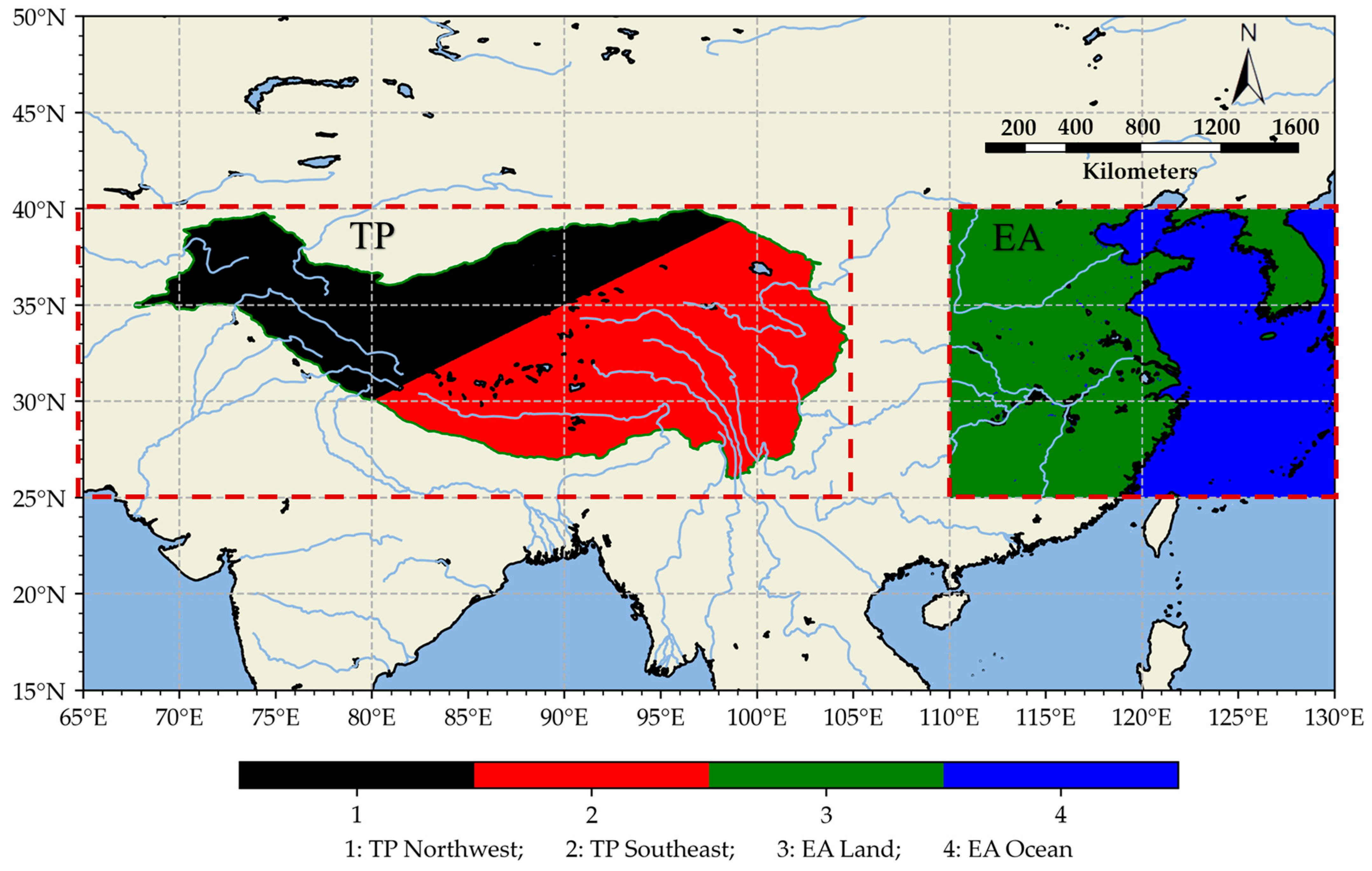
2.1. Study Area

This study focused on the TP (25°N–40°N, 65°E–105°E) and EA (25°N–40°N, 110°E–130°E) at the same latitudes from June to August 2021–2023 (Figure 1). The TP was divided into northwest (black) and southeast (red) subregions based on distinct differences in water vapor conditions and precipitation [30,31]. This division was crucial because the southeast region of the TP receives abundant moisture transport from the South Asian monsoon, leading to a high water vapor content and frequent convective activity [24,32]. In contrast, the northwest region of the TP, being farther from the monsoon-influenced areas, is dominated by dry mid-latitude westerlies, resulting in sparse moisture and suppressed convection. This moisture gradient creates distinct regimes for VDCC development, necessitating separate analysis to unravel region-specific spatiotemporal patterns. The EA was divided into land (green) and ocean (blue) subregions to compare the land–sea differences in VDCCs.

The TP boundary data were obtained from the Integration Dataset of Tibet Plateau Boundary, which provided five boundary types derived from a comprehensive analysis of the Advanced Spaceborne Thermal Emission and Reflection Radiometer Global Digital Elevation Model (ASTER GDEM) and Google Earth remote sensing imagery [33]. For this study, the “TPBoundary_new (2021)” dataset was selected due to its high spatial resolution and accuracy in representing the complex topography of the TP [33].

The TP boundary data are openly available on Big Earth Data Platform for Three Poles at https://doi.org/10.11888/Geogra.tpdc.270099 (accessed on 10 April 2025) or in reference [34].

2.2. GEO-KOMPSAT-2A Data

The Level 1B BT data used in this study were obtained from the new generation geo-satellite GEO-KOMPSAT-2A (GK2A), operated by the Korea Meteorological Administration (KMA). Launched on 4 December 2018, GK2A commenced operational observations at 128.2°E on 25 July 2019 [35]. Since GK2A is located farther west than Himawari-8 (HW8, operated by the Japan Meteorological Agency at 140.7°E), it exhibits advantages in observing VDCCs over the TP. On one hand, large sensor zenith angles (SZAs) will cause uncertainties and errors [36], which are more pronounced in observations from satellites positioned at more eastern. On the other hand, while HW8 covers an operational longitudinal range of 80°E–200°E, the TP’s westernmost boundary (65°E) has exceeded its effective coverage, limiting its utility for comprehensive VDCC monitoring across the entire plateau.

The primary payload Advanced Meteorological Imager (AMI) on board the GK2A is a multi-channel scanning radiometer [35,37]. This advanced instrument, designed for meteorological observations, follows the design principles of the Advanced Baseline Imager (ABI) from the National Oceanic and Atmospheric Administration (NOAA) and the National Aeronautics and Space Administration (NASA) GOES-R satellite [38]. The AMI captures Earth and atmospheric radiation across 16 spectral bands spanning from 0.47 to 13.3 µm (visible to infrared wavelengths), providing enhanced data for monitoring VDCCs compared with previous-generation geo-satellites [35,38]. Additionally, the AMI performs full-disk observations at 10 min intervals, and the infrared band data employed in this study had a spatial resolution of 2 km. This capability enables rapid detection of developing VDCCs and generates extensive datasets for statistical analysis [35].

In addition to BT data from infrared channels, the AMI Level 2 Cloud Detection (ACD) product was utilized to filter out non-cloud targets. The ACD, a cloud mask product developed by the Korea Meteorological Administration’s National Meteorological Satellite Center (NMSC) for GK2A, employs spectral thresholds of BT and brightness temperature difference (BTD) across multiple channels to identify cloud pixels [37,39]. The threshold values were derived through radiative transfer simulations using the TIROS Operational Vertical Sounder (RTTOV) and refined via expert adjustments. Beyond spectral methods, the algorithm incorporated spatial uniformity tests, inversion layer corrections, and top-of-atmosphere (TOA) reflectance validation under clear-sky conditions to improve accuracy [37].

The GK2A data used in this study are available upon request from the NMSC website: http://datasvc.nmsc.kma.go.kr/datasvc/html/main/main.do?lang=en (accessed on 18 January 2024).

2.3. CALIPSO Level 2 Lidar Vertical Feature Mask

In addition to GK2A/AMI observations, this study utilized the Cloud-Aerosol Lidar and Infrared Pathfinder Satellite Observations (CALIPSO) level 2 vertical feature mask (VFM) data (version V4-51) to refine infrared BT and BTD thresholds. By collocating CALIPSO VFM data with GK2A/AMI multi-channel BT observations, we analyzed convective cloud BT/BTD signatures and established region-specific thresholds to exclude non-convective pixels. This synergistic approach leveraged CALIPSO’s high-confidence cloud detection to compensate for ambiguities in passive infrared data alone.

The CALIPSO is a sun-synchronous orbit satellite launched on 28 April 2006. CALIPSO carries the CALIOP (Cloud-Aerosol Lidar with Orthogonal Polarization) instrument, which uses dual-wavelength (532 and 1064 nm) lidar to provide high-resolution vertical profiles of clouds and aerosols. To further remove transparent clouds not associated with VDCCs and snow cover over the mountainous terrain of the TP (which may be misidentified as clouds), the CALIPSO level 2 lidar vertical feature mask (VFM) data product (version V4-51) was used in the study. The VFM describes the vertical and horizontal distribution of cloud and aerosol layers [40,41]. Its data are recorded every 5 km along the satellite ground track, corresponding to observations from 15 consecutive laser pulses. The data have a variable vertical resolution ranging from 30 to 180 m, depending on the altitude [42]. As a lidar-based data product, the VFM is more accurate than passive sensor products in detecting optically thin clouds [43]. Additionally, the cloud detection of the VFM is unaffected by surface snow or ice cover [44], making it a reliable data source in regions with potential snow cover, such as the TP.

The original VFM data are openly available on NASA Langley Atmospheric Science Data Center DAAC at https://doi.org/10.5067/CALIOP/CALIPSO/CAL_LID_L2_VFM-Standard-V4-51 (accessed on 10 April 2025) or in reference [45].

2.4. Precipitation Data from Global Precipitation Measurement

The data from the Global Precipitation Measurement (GPM) mission were used to analyze the difference and relationships between daily variation of VDCCs and precipitation. The Integrated Multi-Satellite Retrievals for GPM (IMERG) data used in this study were named “Final Precipitation L3 Half Hourly 0.1° × 0.1° V07B”, which intercalibrated, merged, and interpolated satellite microwave precipitation estimates with microwave calibrated infrared (IR) satellite estimates to produce global surface precipitation rates at a high resolution of 0.1° every 30 min [46]. As the successor to the Tropical Rainfall Measuring Mission (TRMM), GPM extends coverage to higher latitudes and improves the capability to measure light rain, solid precipitation, and the microphysical properties of precipitating particles [47,48]. The advanced dual-frequency precipitation radar and GPM microwave imager allow GPM to measure the precipitation intensity and type through all cloud layers using a wider data swath [48,49].

The original GPM data presented in the study are openly available at Goddard Earth Sciences Data and Information Services Center at https://doi.org/10.5067/GPM/IMERG/3B-HH/07 (accessed on 10 April 2025) or in reference [50].

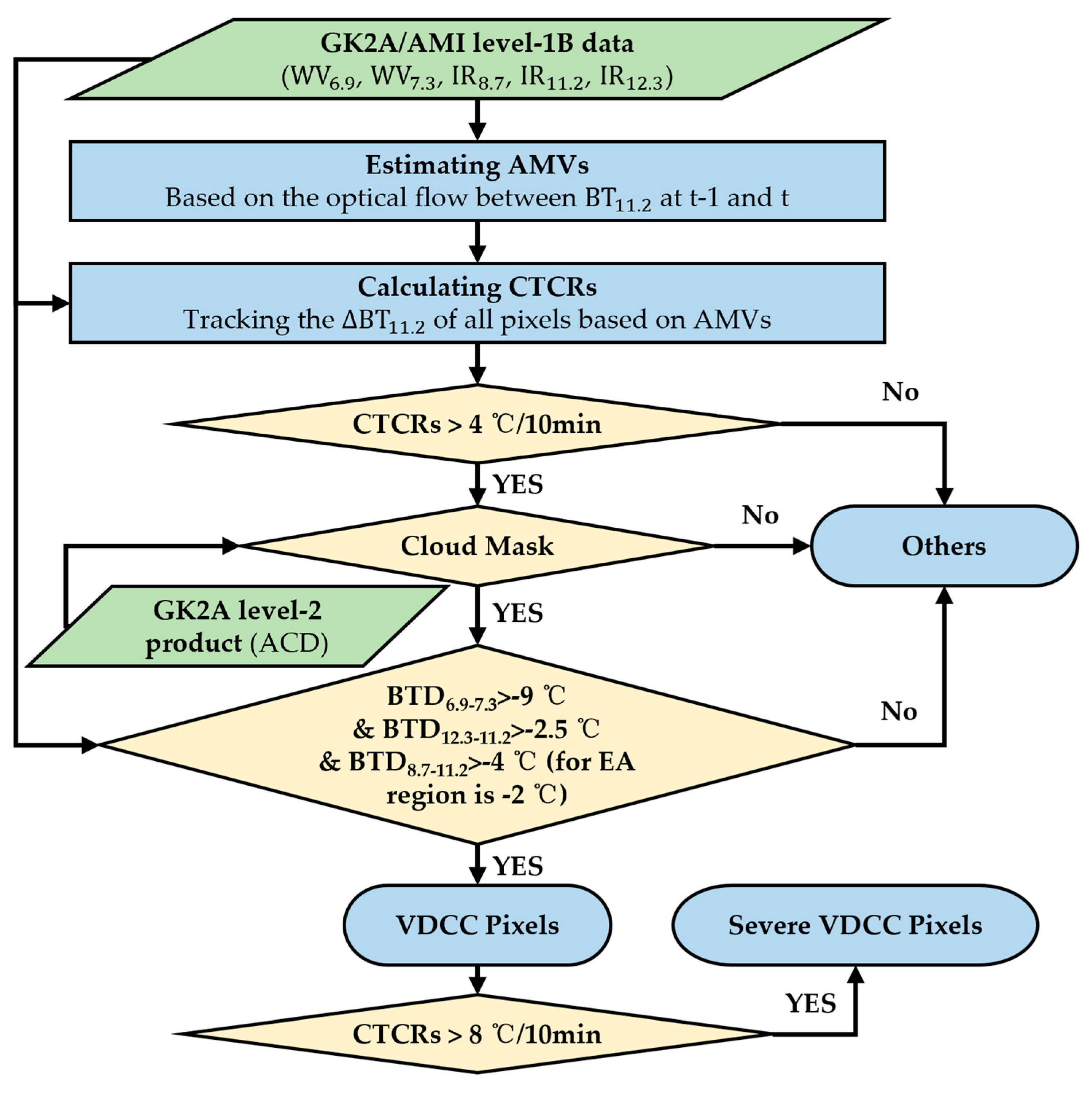
3. Detection of VDCCs

In this study, we achieved all-day, continuous pixel-level monitoring of VDCCs using geo-satellites. This provided a basic dataset for subsequent large-scale statistical analyses of VDCCs’ spatiotemporal distribution characteristics. In this study, VDCC pixels were defined as convective cloud pixels exhibiting significant CTCRs, which correlated with strong vertical velocities in developing convection. The detection of VDCCs consisted of two main parts:

• Tracking all pixels using dense optical flow and calculating the corresponding unfiltered CTCRs.
• Filtering out non-cloud pixels using cloud masks from the ACD product, followed by excluding non-convective cloud pixels through region-specific refined BT and BTD thresholds. These thresholds were determined by matching VFM data with AMI infrared observations, tailored to the TP and EA regions.

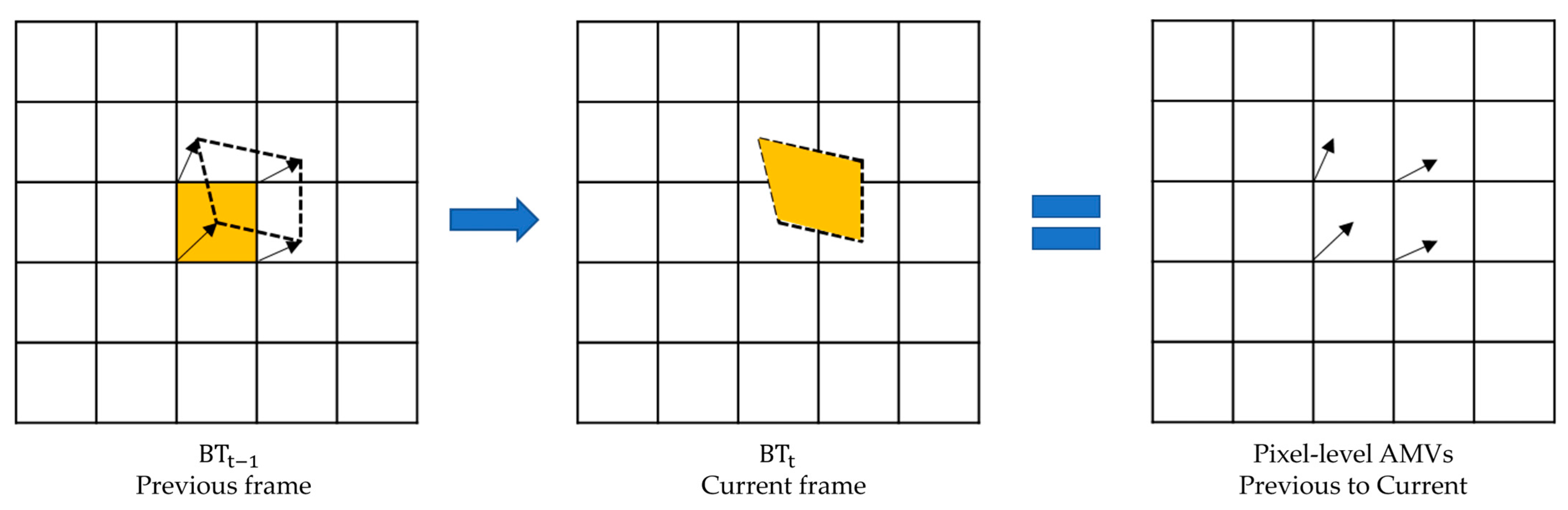
3.1. Pixel-Level Tracking Based on Dense Optical Flow

For VDCCs, the rapidly growing cloud tops are a main feature, manifesting as significant CTCRs in satellite observations. Accurate CTCR calculation requires precise tracking of cloud displacement between consecutive scans using pixel-level atmospheric motion vectors (AMVs). In this study, the optical flow method combined with the rapid scan of satellite was employed to derive the AMVs [51,52].

The optical flow was defined as the motion of image brightness patterns in sequential images, which was calculated based on various constraint equations [18,53]. Optical flow’s capacity to resolve non-rigid cloud motions in complex scenarios, which was critical for capturing the dynamic growth of VDCCs, enabled precise tracking while maintaining computational efficiency [53,54]. By establishing correspondence between cloud pixels across successive observations, the optical flow method provided a foundation for reliable CTCR-based VDCC detection. Figure 2 illustrates the schematic of the optical flow method.

In the study, we estimated the optical flow based on polynomial expansion proposed by Farnebäck (2001, 2003) [55,56]. It utilized polynomial expansion to approximate each small window in two consecutive frames as a quadratic polynomial. The core formula is

$$f\left(\mathit{x}\right)~{\mathit{x}}^T\mathit{A}\mathit{x}+{\mathit{b}}^T\mathit{x}+c$$

(1)

Here, $f\left(\mathit{x}\right)$ represents the image intensity within a polynomial expansion window (PEW), $\mathit{A}$ is a symmetric matrix, $\mathit{b}$ is a vector, c is a scalar, and $\mathit{x}$ is the position vector of the pixel. Assuming pixel displacement $\mathit{d}$ between two frames, the optical flow constraint is expressed as

$$f_2\left(\mathit{x}\right)=f_1\left(\mathit{x}-\mathit{d}\right)$$

(2)

Equation (2) embodies the brightness constancy assumption in optical flow. By comparing the polynomial coefficients of consecutive frames, the optical flow equation is derived:

$$({\mathit{A}}_1\left(\mathit{x}\right)+{\mathit{A}}_2\left(\mathit{x}\right))·\mathit{d}\left(\mathit{x}\right)={\mathit{b}}_1\left(\mathit{x}\right)-{\mathit{b}}_2\left(\mathit{x}\right)$$

(3)

The displacement d(x) can be solved from this linear system. However, Equation (3) assumes small motion magnitudes. To address the limitation of capturing large displacements, we employed an iterative image pyramid method [20,57,58], a hierarchical estimation technique based on multi-layer down-sampled images. This approach estimated the optical flow at coarse spatial scales first, then refined it at finer scales, balancing computational efficiency and accuracy. The hierarchical estimation aligned with meteorological principles where large-scale motions often dominate small-scale variations at macroscale levels [20,59]. Figure 3 illustrates the workflow of the image pyramid method.

For a PEW of size $(n\times n)$ and L layers of the pyramid, the maximum AMV (${AMV}_{max}$) (in pixels) that can be captured by the algorithm is given by

$${AMV}_{max}=(n-1)(2^L-1)/2$$

(4)

According to Equation (4), for a 2 km resolution, 10 min intervals from GK2A/AMI, and a PEW of size $(n=7)$, to capture a maximum moving speed of 70 m/s (${AMV}_{max}\cong 21$ pixels), the number of pyramid layers (L) must be at least three.

Based on the inversion of the AMVs, all pixels were tracked, and the unfiltered CTCRs were calculated. The detailed steps are as follows:

• Processing: Normalize the ${\mathrm{B}\mathrm{T}}_{11.2}$ from AMI at the current time (t) and the previous time (t − 1) (10 min interval) to a range of 0~255, and use these as the input brightness images.
• Estimating AMVs: Estimate the pixel-level AMVs from time t − 1 to time t using dense optical flow.
• Tracking pixels: Use the AMVs as the displacement vectors of pixels to calculate the location of all pixels at time t − 1 based on their positions at time t.
• Calculating unfiltered CTCRs: Calculate the ${\mathrm{B}\mathrm{T}}_{11.2}$ cooling rate of all pixels at time t based on tracking, and apply mean filtering to reduce the effect of noise and outliers.

Finally, the unfiltered CTCRs indicated potential VDCCs based on the correlation between cloud-top cooling and cloud-top ascent. In subsequent statistical analyses, considering potential calculation errors, the CTCR threshold used to identify VDCCs was set to values greater than 4 °C/10 min. This threshold corresponded to a vertical velocity exceeding 1 m/s, assuming an average atmospheric lapse rate of 6.5 °C/km, ensuring the reliability of the statistical characteristics of VDCCs [60]. Additionally, a higher threshold of 8 °C/10 min (~2 m/s) was used to identify severe VDCCs [10], enabling comparative analysis of convective updrafts with different intensities in subsequent statistics.

3.2. Eliminating Non-Convective Cloud Pixels

Although tracking avoided false cooling caused by horizontal cloud motion [5], some significant CTCRs still resulted from non-convective processes, such as rapid surface temperature drops, thickening, or overlapping of semi-transparent clouds. To ensure accurate VDCC detection, it was necessary to eliminate these non-convective cloud pixels.

In the study, the ACD product was used to preliminarily eliminate non-cloud targets. However, ACD-identified clouds still included broken, cirrus, and semi-transparent clouds, which were unrelated to VDCCs and required further elimination. Therefore, more stringent infrared BT and BTD filter conditions were needed for the TP and EA regions. This was achieved by first matching CALIPSO’s VFM data with GK2A/AMI’s multi-channel BT data, then analyzing the BT and BTD characteristics of convective clouds identified by VFM, and finally establishing BT and BTD thresholds to exclude non-convective pixels.

To match VFM and BT data, the center profile of each 5 km VFM segment was selected, and the corresponding 2 km BT data were linearly interpolated based on CALIPSO trajectory coordinates. Due to the large distance between the TP and GK2A, GK2A had a high SZA during observation, while CALIPSO was directly above the cloud tops. Thus, geometric correction (GC) was applied to address the parallax between BT and VFM data [61,62]. A detailed description can be found in Appendix A.

Based on the matching of the VFM data and the BT data, the convective clouds pixels at the top of the VFM profiles from June to August 2021–2023 over TP and EA were selected. To ensure the reliability of the analysis, only cloudy features with high and middle confidence were adopted, and the total number of statistical samples was 29,003 over the TP and 14,607 over the EA. The two-dimensional frequency histogram (FH2D) of these pixels’ BT and BTD is shown in Figure 4.

In Figure 4, BT_11.2 (BT of 11.2 μm channel) corresponds to cloud-top temperature and reflects the relative cloud-top height. The characteristics of BTDs are as follows:

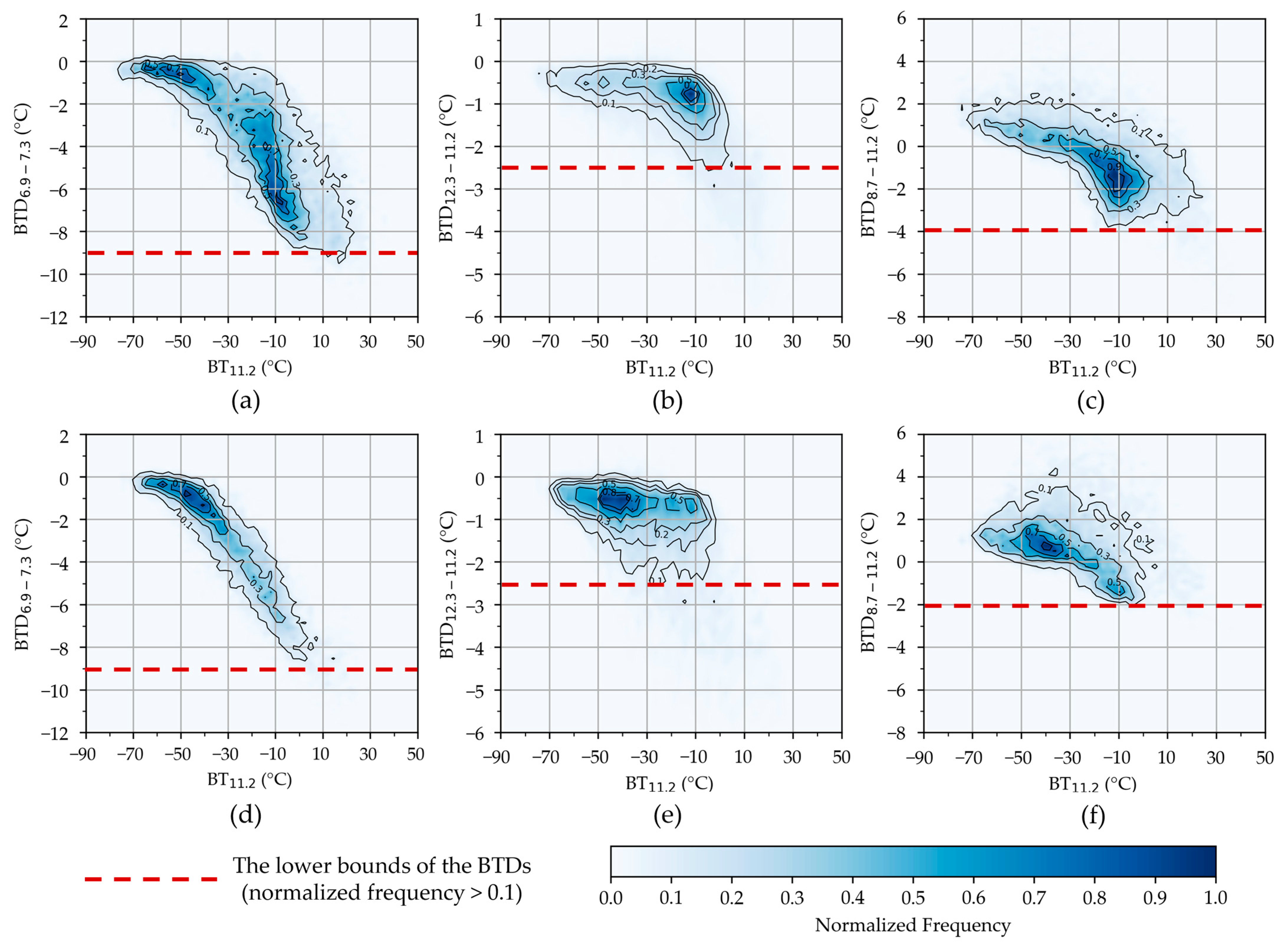
• BTD_6.9−7.3 (BTD between 6.9 and 7.3 μm channels) is derived from adjacent water vapor channels [63,64]. The 6.9 μm channel is strongly absorbed by moisture and primarily responds to upper-layer water vapor. Due to lower water-vapor absorption, the 7.3 μm channel can partially penetrate through upper-level moisture and respond to lower layers. Therefore, the 7.3 μm channel is typically warmer than the 6.9 μm channel, leading to a negative BTD_6.9−7.3 [63]. For rapidly growing convective clouds, upward moisture transport increases upper-level humidity and optical thickness. This simultaneously enhances the absorption of two channels, resulting in a smaller absolute value of their difference and larger BTD_6.9-7.3 values [60].
• BTD_12.3−11.2 (BTD between 12.3 and 11.2 μm channels) is derived from adjacent atmospheric window channels. In clear-sky conditions, this BTD typically shows negative values (below −2 °C) due to the weak water vapor absorption in the 12.3 μm channel (dirty window), and the negative signature becomes more pronounced (below −4 °C) for semi-transparent clouds [63,65]. But for convective clouds, the absolute BTD value progressively approaches 0 K as the cloud-top height increases, the optical thickness grows, and the overlying water vapor decreases [63,66]. Moreover, this BTD can be positive for overshooting and extremely intensive convective clouds that penetrate the tropopause [63]. These numerical variations enable effective discrimination between convective and semi-transparent clouds.
• BTD_8.7−11.2 (BTD between 8.7 and 11.2 μm channels) is related to the phase state of the cloud-top particles [60]. While water and ice exhibit comparable imaginary refractive indices at 8.7 μm, significant divergence occurs at 11.2 μm [60]. This spectral contrast enhances ice cloud absorption relative to water clouds of equivalent water content at 11.2 μm, resulting in negative BTD_8.7−11.2 values for water cloud tops [67]. In contrast, for rapidly growing convective clouds, the glaciation process at the cloud tops will lead to larger BTD_8.7−11.2 values [3].

Based on the above characteristics, the lower bounds of BTDs corresponding to high-frequency regions (normalized frequency > 0.1) in each FH2D (Figure 4) were selected as filter thresholds for VDCCs (marked by red dashed lines).

Table 1. BTD conditions for filtering non-convective cloud pixels over the TP and EA based on AMI observations.

Region	BTD6.9−7.3 (°C)	BTD12.3−11.2 (°C)	BTD8.7−11.2 (°C)
TP	>−9	>−2.5	>−4
EA	>−9	>−2.5	>−2

lists the conditions for filtering non-convective cloud pixels.

In summary, the algorithm flow of VDCCs detection and classification is shown in Figure 5.

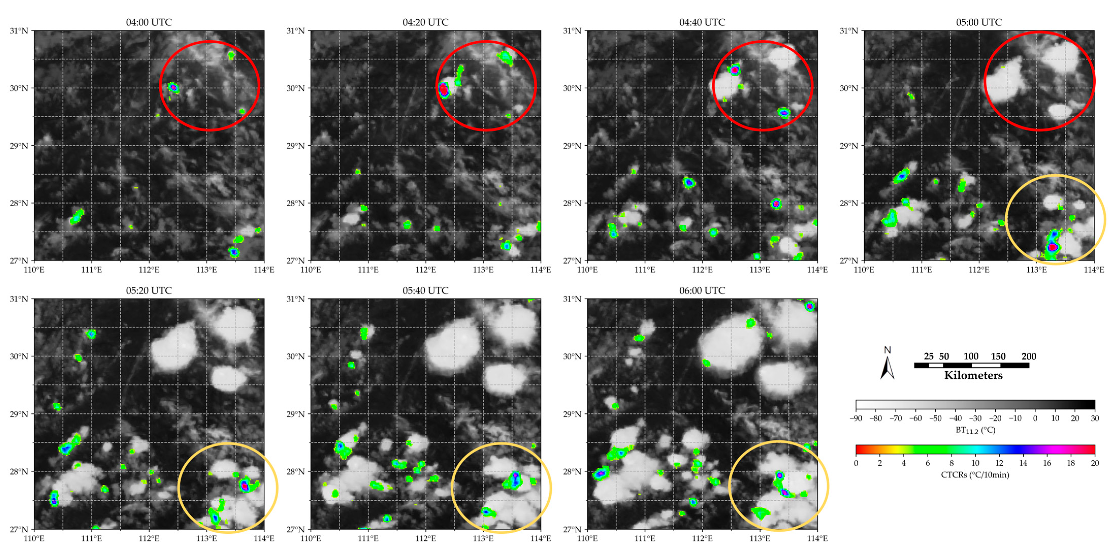
3.3. Detection Results of VDCCs

Figure 6 shows the sequential detection results of VDCCs over the EA region from 04:00 to 06:00 UTC on 20 July 2021. In each frame, actively growing cells exhibit large CTCRs (>4 °C/10 min), reflecting vigorous updrafts. In contrast, mature convective cloud tops with horizontal anvil expansion near the tropopause show small CTCRs due to suppressed vertical growth. This enables the algorithm to distinguish stabilized anvils (CTCRs ≈ 0) from active VDCCs.

As shown in Figure 6, most VDCCs detected at the low level rapidly developed into deeper convective clouds in subsequent frames. For example, three nascent VDCCs (red circles) initiated 40–60 min before reaching maturity, demonstrating the framework’s sensitivity to convective growth. This early detection precedes precipitation and severe weather manifestations, highlighting its potential for early warning systems.

Notably, the algorithm effectively excludes stagnant regions (e.g., the anvil area) while retaining sensitivity to localized reinvigoration (e.g., the new updraft core). For example, a meso-β-scale convective system (MCS, yellow circle) formed through merging convective cells, with new growth zones atop the anvil marked by large CTCRs. These signals, indicative of overshooting tops and convective reinvigoration, correlated with extreme weather events, confirming the algorithm’s ability to detect secondary growth in mature systems.

The algorithm consistently detected both isolated and organized development, validating its robustness across convective regimes. These results illustrated the algorithm’s capability to isolate vertical growth signals across convective lifecycles, establishing a reliable foundation for large-scale statistical analysis of VDCCs.

4. Statistical Analysis of VDCCs

The appearance of VDCCs indicated the development of convection, and their CTCRs reflected the intensity of convection development. Based on satellite monitoring of VDCCs, statistical analyses were conducted on the diurnal variations, horizontal distributions, and vertical distributions of VDCCs over the TP and EA regions during the summers (June to August) from 2021 to 2023. The basic characteristics and differences of convection in each region can be revealed by studying the spatiotemporal distribution of VDCCs.

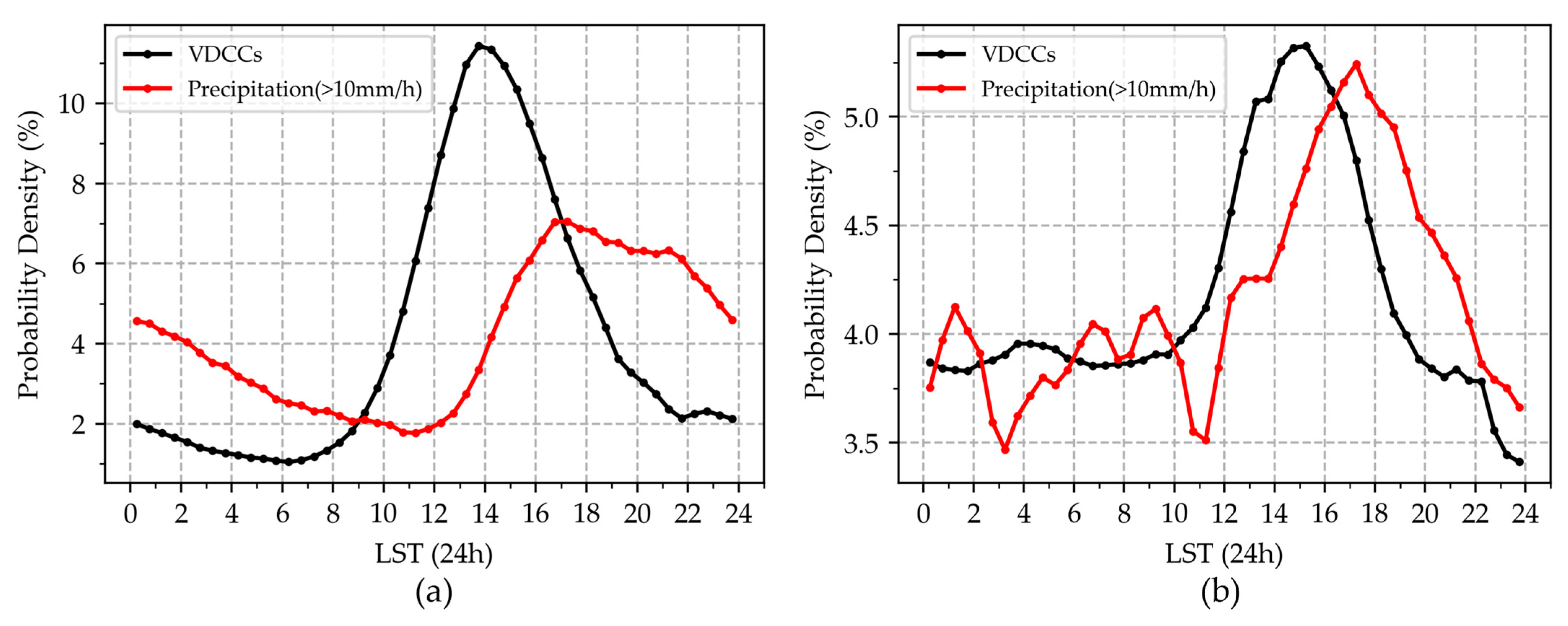
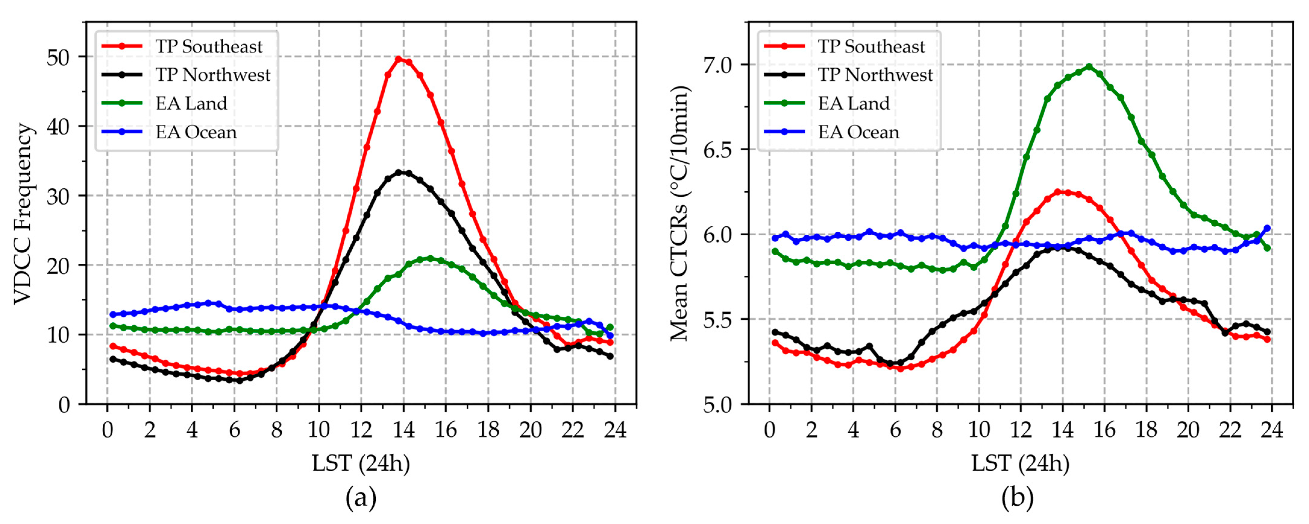
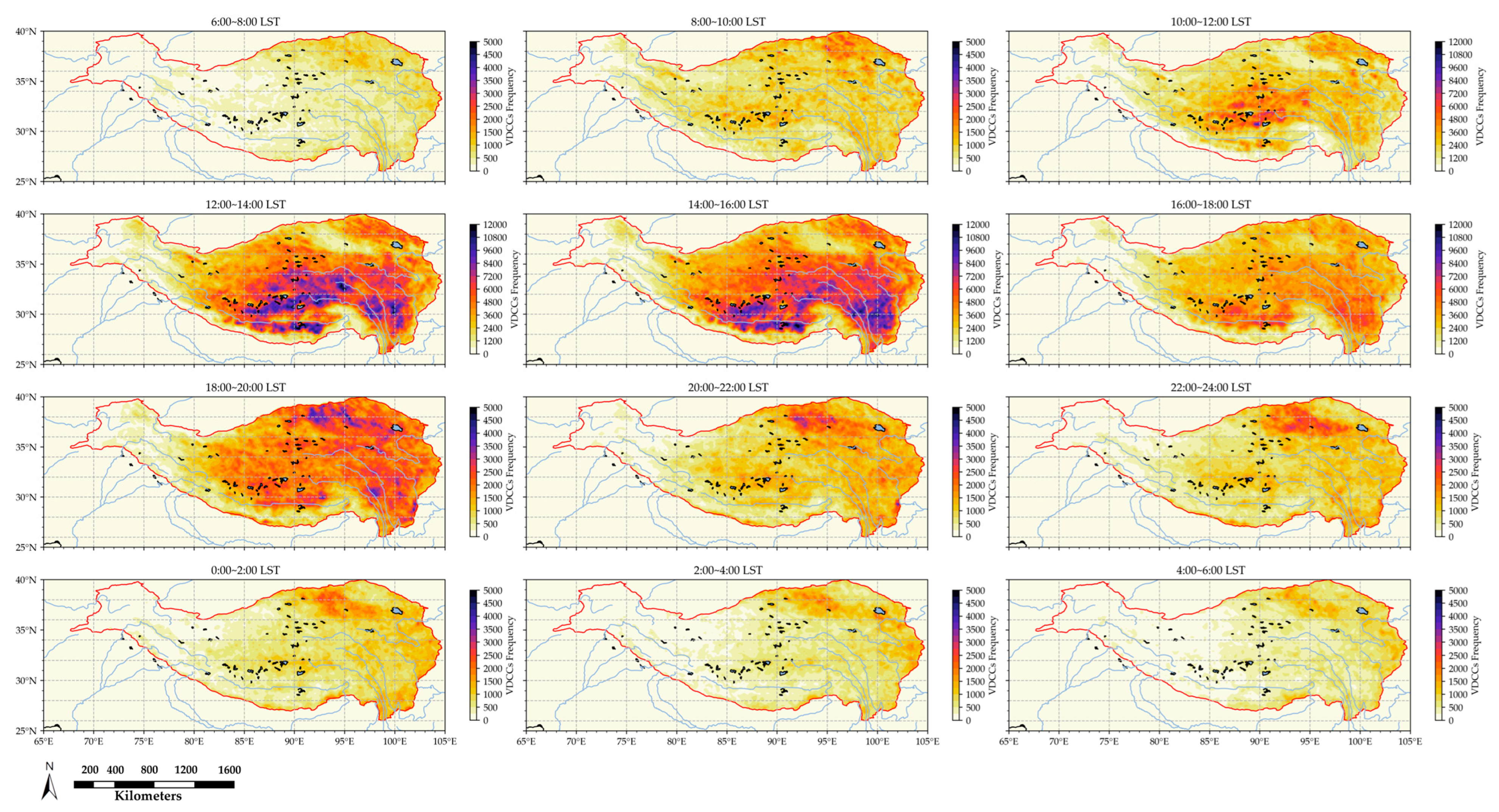
4.1. Diurnal Variation of VDCCs

Figure 7 compares the diurnal variation in the probability density of VDCCs and precipitation. The VDCC probability density was low in the early morning across the TP and EA regions, gradually rose throughout the morning, peaked in the afternoon, and then declined until the next early morning. While the diurnal variation trends of precipitation closely mirrored those of VDCCs, there was a significant difference in the timing of their phases. Specifically, the peak times of precipitation in each region occurred around 17:00. In contrast, the peak time of VDCCs was earlier, occurring at approximately 14:00 over the TP and 15:00 over EA. This indicated that the overall diurnal phase (both the peak and trough) of VDCCs preceded that of precipitation. This difference highlighted VDCCs as an early signal for precipitation, demonstrating their potential application in early warnings of severe convection.

Figure 7 also reveals regional differences in the diurnal phase of VDCCs between the TP and EA. Further statistical analysis of VDCC diurnal variation in subregions is shown in Figure 8. During the day, solar radiation combined with the TP’s high altitude caused the plateau to act as a massive, elevated heat source in summer, heating the middle atmosphere [68]. This intense thermal forcing enhanced the atmospheric instability, making the TP more prone to triggering convection than the lower-lying EA region. This was evident in the earlier diurnal phase and higher afternoon peak of VDCC frequency over the TP compared with EA (Figure 8a). However, limited water vapor content restricted further convective development over the TP, resulting in lower average intensity, as reflected by the lower CTCR peak over the TP than EA (Figure 8b). Influenced by the South Asian monsoon, water vapor content decreased from the southeast to the northwest over the TP [30], leading to more frequent and intense convection in the southeast. This spatial pattern was consistent with the higher frequency and CTCR peaks of VDCCs in the southeast (Figure 8). Over EA, the ocean’s thermal inertia maintained atmospheric instability at night, while stable moisture supply ensured consistent convective strength. Consequently, oceanic VDCCs in EA peaked nocturnally, contrasting with continental diurnal cycles (Figure 8a), and their CTCRs exhibited minimal daily variation (Figure 8b).

The temporal lead in the occurrence of VDCCs compared with precipitation underscores their utility as early indicators of convective storms. Regional contrasts further highlight that the TP exhibits earlier and more frequent convection due to intense thermal forcing, while limited moisture availability restricts the convective intensity.

4.2. Horizontal Distributions of VDCCs

Building on insights into diurnal variations, the horizontal distributions of VDCCs further revealed how local topography and moisture availability modulated convective organization across the TP and EA. Figure 9 illustrates horizontal distributions of VDCC frequency over the TP, which followed a diurnal cycle, with maximum frequency occurring during daytime hours when solar heating was strongest. Meanwhile, the spatial patterns correlated well with regional moisture gradients: during the peak period of convective development in the afternoon, the VDCC frequency decreased from the southeast to the northwest, which corresponded to the decrease in water vapor distribution from the southeast to the northwest over the TP due to the influence of the South Asian monsoon.

Notably, localized geographic features led to distinct convective development patterns. For example, over the central TP, the presence of extensive lakes and wetlands enhanced the surface latent heat flux, leading to earlier boundary layer destabilization and consequently producing the earlier convective onset in the morning (10:00–12:00 LST). In addition, the Qaidam Basin (an enclosed basin in the northeastern TP) exhibited delayed convective activity, maintaining higher VDCC frequency at night. This anomaly was probably due to its enclosed basin topography: daytime heat retention sustained near-surface instability, while nighttime cold air from surrounding mountains enhanced mechanical lifting.

Figure 10 presents the horizontal distributions of the VDCC frequency over the EA. Land regions exhibited afternoon maxima, particularly in southeastern coastal areas where solar heating combined with orographic effects: strong daytime surface sensible heat flux enhanced convective instability, while the hilly terrain mechanically forced low-level airflow ascent. In contrast, oceanic regions showed nocturnal maxima due to the ocean’s thermal inertia: the slower cooling rate of the sea surface relative to land maintained higher sensible and latent heat fluxes at night. Additionally, the nighttime land–sea temperature gradient further drove low-level moisture transport toward the ocean, maintaining boundary layer instability over marine areas.

The Korean Peninsula exhibited persistently high VDCC frequency throughout the day, a feature tied to its transitional location between continental and maritime air masses [69]. Summer southerly monsoonal flow transported oceanic moisture inland, converging with drier continental air to form semi-stationary frontal zones. Local topography (e.g., Taebaek Mountains) further amplified moisture convergence and convective triggering through mechanical uplift.

These spatial patterns highlight the influence of local terrain and monsoon-driven moisture conditions on VDCCs and convection development. The next section explores the vertical distribution of VDCCs to understand how these regional differences manifest in the vertical development of convection.

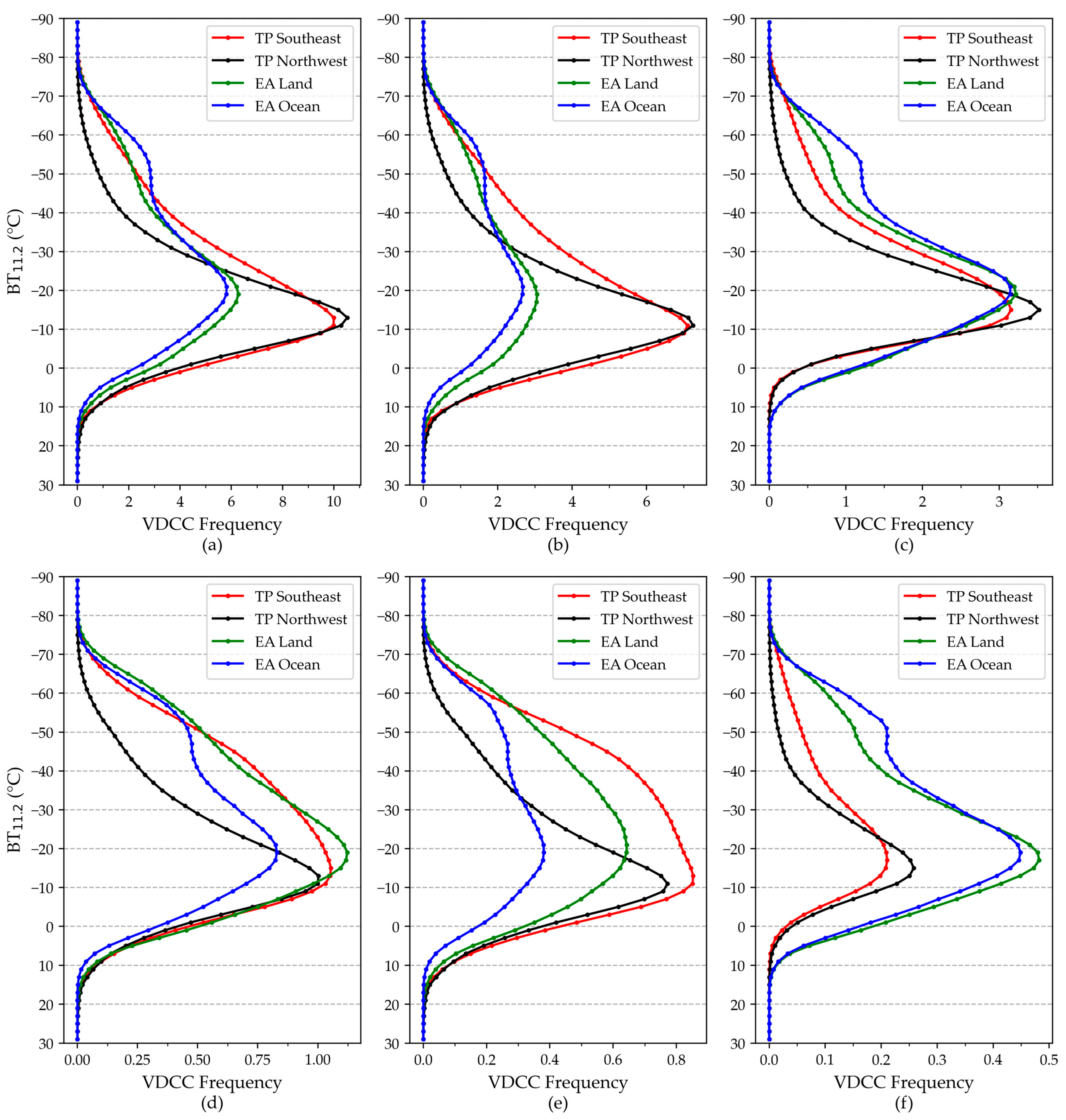
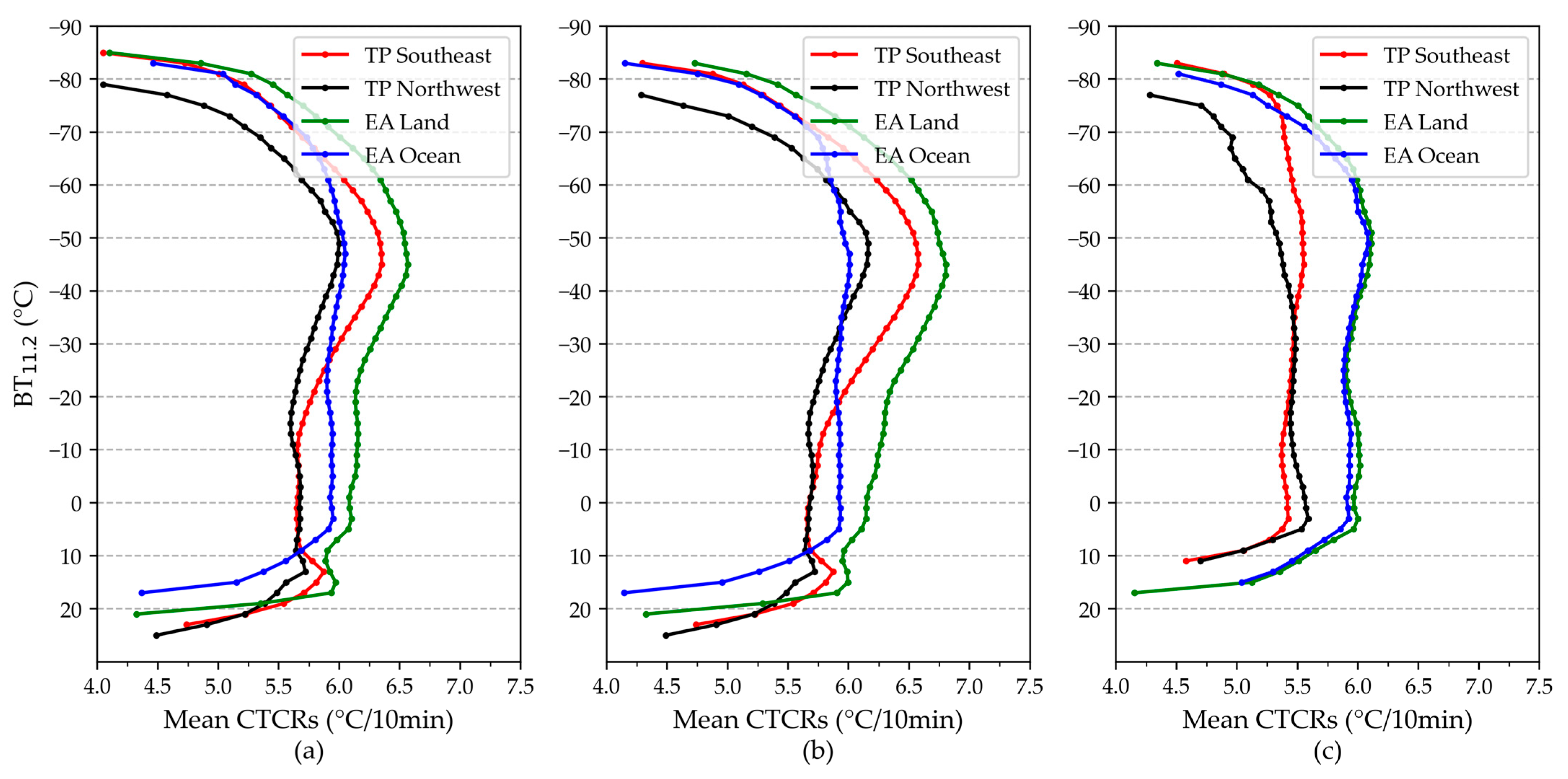
4.3. Vertical Distribution of VDCCs

Beyond horizontal gradients, the vertical stratification of VDCCs unveils the lifecycle of convective systems and exposes fundamental constraints on convective growth, linking near-surface triggers to upper-tropospheric outcomes. In this section, the vertical distribution characteristics of VDCCs over different subregions are further statistically compared. Figure 11 shows the vertical frequency distribution of VDCCs in different subregions. In Figure 11, the BT_11.2 observed by AMI is used to indicate the relative altitude of VDCCs (the higher the altitude, the lower the BT_11.2 value). As illustrated in Figure 11a–c, over the TP, VDCC frequency peaked near the −10 °C level, whereas EA showed a dominant peak at −20 °C. They corresponded to cumulus accumulation as described in Johnson et al. (1999) [70] and Luo et al. (2009) [71]. The melting level (~0 °C) acted as a weak stable layer that inhibited convective development [70]. At this level, VDCCs that ceased growth at the mid-level coexisted with those that continued to ascend, resulting in the observed frequency maxima [8,71]. The higher peak locations (relative to the melting level) were likely due to detection criteria (Section 3.2) favoring actively developing VDCCs.

In Figure 11b, the TP exhibits a significantly higher frequency of VDCCs at mid-to-low levels during daytime compared with the EA, highlighting the dominant role of intense thermal forcing over the plateau in convection development. However, the TP’s VDCC frequency declined sharply above the peak level, in contrast to the EA’s gradual decrease. This disparity suggested that a greater proportion of VDCCs over the EA sustained ascent into the upper troposphere. Additionally, frequency subpeaks near the tropopause (−50 °C to −60 °C) were observed over EA regions, particularly in oceanic areas with abundant water vapor supply. These subpeaks were associated with the continuous development of mature convective clouds and cloud-top overshooting, indicating more active deep convection over the EA. Over the TP, although vigorous daytime heating initiated prolific low-level convection, limited moisture availability and dry-air entrainment restricted vertical cloud development, thereby reducing precipitation efficiency.

For severe VDCCs (CTCRs > 8 K/10 min; Figure 11d–f), the southeastern TP (characterized by higher moisture content) displayed slower frequency decay above the peak level compared with the arid northwestern TP. This contrast implied that moisture availability critically modulated the probability of continuous VDCC development despite similar initial thermal forcing. Diurnal analysis further showed that severe VDCCs over the southeastern TP, energized by daytime heating (Figure 11e,f), exhibited higher peak frequencies than those in EA but underwent rapid nocturnal decay, particularly at upper-tropospheric levels. In contrast, EA’s severe VDCCs maintained relatively stable vertical distributions across day and night, reflecting the persistent influence of monsoonal moisture and synoptic-scale lifting.

Figure 12 presents vertical profiles of the mean CTCRs of VDCCs, capturing convective intensity evolution during development. In the lower troposphere, CTCRs initially increased rapidly due to convective initiation driven by thermal or dynamic forcing. As VDCCs surpassed the aggregation height of frequent occurrence (the VDCC frequency peak was −10 °C over the TP and −20 °C over EA, as shown in Figure 11) and continued ascending, they entered a mixed-phase layer where coexisting supercooled water and ice crystals enhanced buoyancy via latent heat release from freezing and deposition. This process sustained rapid CTCR increase until peaking near the equilibrium level, followed by a gradual decline due to tropopause suppression.

Land–ocean contrasts revealed that marine VDCCs grew more slowly in the mid-levels and exhibited smaller diurnal variations (Figure 12b,c). This occurred because deeper moisture layers over oceans produced smaller buoyancy contrasts from latent heat release, unlike drier mid-level air over land. Additionally, stable marine evaporation weakened diurnal CTCR variability.

Notably, while the northwestern and southeastern TP showed similar CTCR trends during the initial ascent, the southeastern TP (with monsoonal moisture supply) showed higher peak values of CTCRs and more frequent upper-level intense VDCCs. This disparity underscored the critical role of low-level humidity in modulating latent heat release and vertical development.

These vertical profiles, combined with diurnal and horizontal analyses, offer a comprehensive view of how thermal forcing, topography, and moisture availability collectively shape the development and intensity of VDCCs. This combination enhances our understanding of convective processes over the TP and EA.

5. Conclusions

This study established VDCCs as pivotal markers of convective evolution and revealed the feasibility of detecting vertically developing convective signals by integrating optical flow-based atmospheric motion tracking with CTCR calculation, leveraging the high spatiotemporal resolution and multispectral capabilities of the GK2A satellite. The combination of dense optical flow vectors and CTC thresholds enabled robust pixel-level identification of VDCCs at 10 min intervals, effectively isolating early-stage convective signals from complex cloud motions.

Diurnal variation statistics indicated that VDCCs served as precursors to severe convective weather, with their diurnal frequency peaks occurring 2–3 h before precipitation. Horizontal distribution analyses highlighted how regional topography and moisture gradients influenced the VDCC frequency. Vertical distribution analyses further revealed distinct convective development regimes across regions: over the TP, the VDCC frequency peaked at mid-low levels due to intense thermal forcing but exhibited rapid vertical decay, while over EA, VDCCs penetrated deeper into the upper troposphere (−50 °C to −60 °C), sustained by monsoonal moisture (Figure 11). These vertical contrasts demonstrated how moisture availability and entrainment governed convective depth and intensity—findings unattainable through horizontal or diurnal statistics alone. Specifically, the weaker vertical penetration over the TP likely resulted from drier atmospheric conditions and stronger entrainment of ambient air, whereas the deeper convection over EA was facilitated by abundant low-level moisture from monsoonal flows and weaker mid-level inhibition. Sub-regional and land–ocean differences further highlight the roles of topography, moisture availability, and thermal inertia in modulating convective activity.

By advancing VDCC monitoring capabilities and our understanding of VDCC dynamics, this study provides foundational insights for improving severe weather nowcasting and convective parameterizations in climate models. It should be noted that this research primarily focused on general summer convective characteristics using data from three consecutive summers (2021–2023) and thus did not address the interannual variability influence in convective distribution patterns by large-scale climate modes like ENSO or monsoon strength variation in the long-time period. Future studies incorporating extended temporal scales will be critical to generalize these findings.

References

1. Li, P.; Moseley, C.; Prein, A.F.; Chen, H.; Li, J.; Furtado, K.; Zhou, T. Mesoscale Convective System Precipitation Characteristics over East Asia. Part I: Regional Differences and Seasonal Variations. J. Clim. 2020, 33, 9271–9286. [Google Scholar] [CrossRef]
2. Yang, Y.; Zhao, C.; Sun, Y.; Chi, Y.; Fan, H. Convective Cloud Detection and Tracking Using the New-Generation Geostationary Satellite Over South China. IEEE Trans. Geosci. Remote Sens. 2023, 61, 4103912. [Google Scholar] [CrossRef]
3. Senf, F.; Deneke, H. Satellite-Based Characterization of Convective Growth and Glaciation and Its Relationship to Precipitation Formation over Central Europe. J. Appl. Meteorol. Climatol. 2017, 56, 1827–1845. [Google Scholar] [CrossRef]
4. Adler, R.F.; Fenn, D.D. Thunderstorm Vertical Velocities Estimated from Satellite Data. J. Atmos. Sci. 1979, 36, 1747–1754. [Google Scholar] [CrossRef]
5. Sieglaff, J.M.; Cronce, L.M.; Feltz, W.F.; Bedka, K.M.; Pavolonis, M.J.; Heidinger, A.K. Nowcasting Convective Storm Initiation Using Satellite-Based Box-Averaged Cloud-Top Cooling and Cloud-Type Trends. J. Appl. Meteorol. Climatol. 2011, 50, 110–126. [Google Scholar] [CrossRef]
6. Hartung, D.C.; Sieglaff, J.M.; Cronce, L.M.; Feltz, W.F. An Intercomparison of UW Cloud-Top Cooling Rates with WSR-88D Radar Data. Weather. Forecast. 2013, 28, 463–480. [Google Scholar] [CrossRef]
7. Mecikalski, J.R.; Jewett, C.P.; Apke, J.M.; Carey, L.D. Analysis of Cumulus Cloud Updrafts as Observed with 1-Min Resolution Super Rapid Scan GOES Imagery. Mon. Weather. Rev. 2016, 144, 811–830. [Google Scholar] [CrossRef]
8. Luo, Z.J.; Jeyaratnam, J.; Iwasaki, S.; Takahashi, H.; Anderson, R. Convective Vertical Velocity and Cloud Internal Vertical Structure: An A-Train Perspective. Geophys. Res. Lett. 2014, 41, 723–729. [Google Scholar] [CrossRef]
9. Adler, R.F.; Markus, M.J.; Fenn, D.D. Detection of Severe Midwest Thunderstorms Using Geosynchronous Satellite Data. Mon. Weather. Rev. 1985, 113, 769–781. [Google Scholar] [CrossRef]
10. Roberts, R.D.; Rutledge, S. Nowcasting Storm Initiation and Growth Using GOES-8 and WSR-88D Data. Weather. Forecast. 2003, 18, 562–584. [Google Scholar] [CrossRef]
11. Sieglaff, J.M.; Hartung, D.C.; Feltz, W.F.; Cronce, L.M.; Lakshmanan, V. A Satellite-Based Convective Cloud Object Tracking and Multipurpose Data Fusion Tool with Application to Developing Convection. J. Atmos. Ocean. Technol. 2013, 30, 510–525. [Google Scholar] [CrossRef]
12. Sieglaff, J.M.; Cronce, L.M.; Feltz, W.F. Improving Satellite-Based Convective Cloud Growth Monitoring with Visible Optical Depth Retrievals. J. Appl. Meteorol. Climatol. 2014, 53, 506–520. [Google Scholar] [CrossRef]
13. Mecikalski, J.R.; Bedka, K.M. Forecasting Convective Initiation by Monitoring the Evolution of Moving Cumulus in Daytime GOES Imagery. Mon. Weather. Rev. 2006, 134, 49–78. [Google Scholar] [CrossRef]
14. Siewert, C.W.; Koenig, M.; Mecikalski, J.R. Application of Meteosat Second Generation Data towards Improving the Nowcasting of Convective Initiation. Meteorol. Appl. 2010, 17, 442–451. [Google Scholar] [CrossRef]
15. Mecikalski, J.R.; MacKenzie, W.M.; Koenig, M.; Muller, S. Cloud-Top Properties of Growing Cumulus Prior to Convective Initiation as Measured by Meteosat Second Generation. Part I: Infrared Fields. J. Appl. Meteorol. Climatol. 2010, 49, 521–534. [Google Scholar] [CrossRef]
16. Walker, J.R.; MacKenzie, W.M.; Mecikalski, J.R.; Jewett, C.P. An Enhanced Geostationary Satellite–Based Convective Initiation Algorithm for 0–2-h Nowcasting with Object Tracking. J. Appl. Meteorol. Climatol. 2012, 51, 1931–1949. [Google Scholar] [CrossRef]
17. Mecikalski, J.R.; Williams, J.K.; Jewett, C.P.; Ahijevych, D.; LeRoy, A.; Walker, J.R. Probabilistic 0–1-h Convective Initiation Nowcasts That Combine Geostationary Satellite Observations and Numerical Weather Prediction Model Data. J. Appl. Meteorol. Climatol. 2015, 54, 1039–1059. [Google Scholar] [CrossRef]
18. Vandal, T.J.; Duffy, K.; McCarty, W.; Sewnath, A.; Nemani, R. Dense Feature Tracking of Atmospheric Winds with Deep Optical Flow. In Proceedings of the 28th ACM SIGKDD Conference on Knowledge Discovery and Data Mining, Washington, DC, USA, 14–18 August 2022; ACM: New York, NY, USA, 2022; pp. 1807–1815. [Google Scholar]
19. Posselt, D.J.; Wu, L.; Mueller, K.; Huang, L.; Irion, F.W.; Brown, S.; Su, H.; Santek, D.; Velden, C.S. Quantitative Assessment of State-Dependent Atmospheric Motion Vector Uncertainties. J. Appl. Meteorol. Climatol. 2019, 58, 2479–2495. [Google Scholar] [CrossRef]
20. Wu, Q.; Wang, H.-Q.; Lin, Y.-J.; Zhuang, Y.-Z.; Zhang, Y. Deriving AMVs from Geostationary Satellite Images Using Optical Flow Algorithm Based on Polynomial Expansion. J. Atmos. Ocean. Technol. 2016, 33, 1727–1747. [Google Scholar] [CrossRef]
21. Bedka, K.M.; Wang, C.; Rogers, R.; Carey, L.D.; Feltz, W.; Kanak, J. Examining Deep Convective Cloud Evolution Using Total Lightning, WSR-88D, and GOES-14 Super Rapid Scan Datasets. Weather. Forecast. 2015, 30, 571–590. [Google Scholar] [CrossRef]
22. Zheng, D.; Zhang, Y.; Zhang, Y.; Yao, W.; Wang, F.; Lyu, W.; Meng, Q.; Fan, X.; Ma, Y.; Yang, J. Lightning and Deep Convective Activities over the Tibetan Plateau. Natl. Sci. Rev. 2020, 7, 487–488. [Google Scholar] [CrossRef] [PubMed]
23. Li, J.; Yue, Z.; Lu, C.; Chen, J.; Wu, X.; Xu, X.; Luo, S.; Zhu, L.; Wu, S.; Wang, F.; et al. Convective Entrainment Rate over the Tibetan Plateau and Its Adjacent Regions in the Boreal Summer Using SNPP-VIIRS. Remote Sens. 2022, 14, 2073. [Google Scholar] [CrossRef]
24. Li, J.; Lu, C.; Chen, J.; Zhou, X.; Yang, K.; Li, J.; Wu, X.; Xu, X.; Wu, S.; Hu, R.; et al. The Influence of Complex Terrain on Cloud and Precipitation on the Foot and Slope of the Southeastern Tibetan Plateau. Clim. Dyn. 2024, 62, 3143–3163. [Google Scholar] [CrossRef]
25. Fu, Y.; Ma, Y.; Zhong, L.; Yang, Y.; Guo, X.; Wang, C.; Xu, X.; Yang, K.; Xu, X.; Liu, L.; et al. Land-Surface Processes and Summer-Cloud-Precipitation Characteristics in the Tibetan Plateau and Their Effects on Downstream Weather: A Review and Perspective. Natl. Sci. Rev. 2020, 7, 500–515. [Google Scholar] [CrossRef]
26. Zhang, G.; Mao, J.; Liu, Y.; Wu, G. PV Perspective of Impacts on Downstream Extreme Rainfall Event of a Tibetan Plateau Vortex Collaborating with a Southwest China Vortex. Adv. Atmos. Sci. 2021, 38, 1835–1851. [Google Scholar] [CrossRef]
27. Chen, L.; Reiter, E.R.; Feng, Z. The Atmospheric Heat Source over the Tibetan Plateau: May–August 1979. Mon. Weather. Rev. 1985, 113, 1771–1790. [Google Scholar] [CrossRef]
28. Wu, G.; Zhang, Y. Tibetan Plateau Forcing and the Timing of the Monsoon Onset over South Asia and the South China Sea. Mon. Weather. Rev. 1998, 126, 913–927. [Google Scholar] [CrossRef]
29. Zhao, Y.; Xu, X.; Liu, L.; Zhang, R.; Xu, H.; Wang, Y.; Li, J. Effects of Convection over the Tibetan Plateau on Rainstorms Downstream of the Yangtze River Basin. Atmos. Res. 2019, 219, 24–35. [Google Scholar] [CrossRef]
30. Kukulies, J.; Chen, D.; Wang, M. Temporal and Spatial Variations of Convection, Clouds and Precipitation over the Tibetan Plateau from Recent Satellite Observations. Part II: Precipitation Climatology Derived from Global Precipitation Measurement Mission. Int. J. Climatol. 2020, 40, 4858–4875. [Google Scholar] [CrossRef]
31. Li, D.; Yang, K.; Tang, W.; Li, X.; Zhou, X.; Guo, D. Characterizing Precipitation in High Altitudes of the Western Tibetan Plateau with a Focus on Major Glacier Areas. Int. J. Climatol. 2020, 40, 5114–5127. [Google Scholar] [CrossRef]
32. Xu, X.; Heng, Z.; Li, Y.; Wang, S.; Li, J.; Wang, Y.; Chen, J.; Zhang, P.; Lu, C. Improvement of Cloud Microphysical Parameterization and Its Advantages in Simulating Precipitation along the Sichuan-Xizang Railway. Sci. China Earth Sci. 2024, 67, 856–873. [Google Scholar] [CrossRef]
33. Zhang, Y.; Li, B.; Liu, L.; Zheng, D. Redetermine the Region and Boundaries of Tibetan Plateau. Geogr. Res. 2021, 40, 1543–1553. [Google Scholar] [CrossRef]
34. Zhang, Y. Integration Dataset of Tibet Plateau Boundary. National Tibetan Plateau/Third Pole Environment Data Center. Available online: https://data.tpdc.ac.cn/en/data/61701a2b-31e5-41bf-b0a3-607c2a9bd3b3/ (accessed on 10 April 2025).
35. Kim, D.; Gu, M.; Oh, T.-H.; Kim, E.-K.; Yang, H.-J. Introduction of the Advanced Meteorological Imager of Geo-Kompsat-2a: In-Orbit Tests and Performance Validation. Remote Sens. 2021, 13, 1303. [Google Scholar] [CrossRef]
36. Chen, D.; Guo, J.; Wang, H.; Li, J.; Min, M.; Zhao, W.; Yao, D. The Cloud Top Distribution and Diurnal Variation of Clouds Over East Asia: Preliminary Results from Advanced Himawari Imager. J. Geophys. Res. Atmos. 2018, 123, 3724–3739. [Google Scholar] [CrossRef]
37. Lee, S.; Choi, J. Daytime Cloud Detection Algorithm Based on a Multitemporal Dataset for GK-2A Imagery. Remote Sens. 2021, 13, 3215. [Google Scholar] [CrossRef]
38. Jang, J.-C.; Lee, S.; Sohn, E.-H.; Noh, Y.-J.; Miller, S.D. Combined Dust Detection Algorithm for Asian Dust Events Over East Asia Using GK2A/AMI: A Case Study in October 2019. Asia Pac. J. Atmos. Sci. 2022, 58, 45–64. [Google Scholar] [CrossRef]
39. Chung, S.-R.; Ahn, M.-H.; Han, K.-S.; Lee, K.-T.; Shin, D.-B. Meteorological Products of Geo-KOMPSAT 2A (GK2A) Satellite. Asia Pac. J. Atmos. Sci. 2020, 56, 185. [Google Scholar] [CrossRef]
40. Liu, Z.; Vaughan, M.; Winker, D.; Kittaka, C.; Getzewich, B.; Kuehn, R.; Omar, A.; Powell, K.; Trepte, C.; Hostetler, C. The CALIPSO Lidar Cloud and Aerosol Discrimination: Version 2 Algorithm and Initial Assessment of Performance. J. Atmos. Ocean. Technol. 2009, 26, 1198–1213. [Google Scholar] [CrossRef]
41. Vaughan, M.A.; Powell, K.A.; Winker, D.M.; Hostetler, C.A.; Kuehn, R.E.; Hunt, W.H.; Getzewich, B.J.; Young, S.A.; Liu, Z.; McGill, M.J. Fully Automated Detection of Cloud and Aerosol Layers in the CALIPSO Lidar Measurements. J. Atmos. Ocean. Technol. 2009, 26, 2034–2050. [Google Scholar] [CrossRef]
42. Winker, D.M.; Vaughan, M.A.; Omar, A.; Hu, Y.; Powell, K.A.; Liu, Z.; Hunt, W.H.; Young, S.A. Overview of the CALIPSO Mission and CALIOP Data Processing Algorithms. J. Atmos. Ocean. Technol. 2009, 26, 2310–2323. [Google Scholar] [CrossRef]
43. Hagihara, Y.; Okamoto, H.; Yoshida, R. Development of a Combined CloudSat-CALIPSO Cloud Mask to Show Global Cloud Distribution. J. Geophys. Res. Atmos. 2010, 115, D00H33. [Google Scholar] [CrossRef]
44. Delanoë, J.; Hogan, R.J. Combined CloudSat-CALIPSO-MODIS Retrievals of the Properties of Ice Clouds. J. Geophys. Res. Atmos. 2010, 115, D00H29. [Google Scholar] [CrossRef]
45. NASA/LARC/SD/ASDC. CALIPSO Lidar Level 2 Vertical Feature Mask (VFM), V4-51. NASA Langley Atmospheric Science Data Center DAAC. Available online: https://asdc.larc.nasa.gov/project/CALIPSO/CAL_LID_L2_VFM-Standard-V4-51_V4-51 (accessed on 10 April 2025).
46. Wang, Y.; Li, Z.; Gao, L.; Zhong, Y.; Peng, X. Comparison of GPM IMERG Version 06 Final Run Products and Its Latest Version 07 Precipitation Products across Scales: Similarities, Differences and Improvements. Remote Sens. 2023, 15, 5622. [Google Scholar] [CrossRef]
47. Skofronick-Jackson, G.; Kulie, M.; Milani, L.; Munchak, S.J.; Wood, N.B.; Levizzani, V. Satellite Estimation of Falling Snow: A Global Precipitation Measurement (GPM) Core Observatory Perspective. J. Appl. Meteorol. Climatol. 2019, 58, 1429–1448. [Google Scholar] [CrossRef]
48. Skofronick-Jackson, G.; Kirschbaum, D.; Petersen, W.; Huffman, G.; Kidd, C.; Stocker, E.; Kakar, R. The Global Precipitation Measurement (GPM) Mission’s Scientific Achievements and Societal Contributions: Reviewing Four Years of Advanced Rain and Snow Observations. Q. J. R. Meteorol. Soc. 2018, 144, 27–48. [Google Scholar] [CrossRef]
49. Liu, Z.; Ostrenga, D.; Vollmer, B.; Deshong, B.; Macritchie, K.; Greene, M.; Kempler, S. Global Precipitation Measurement Mission Products and Services at the NASA GES DISC. Bull. Am. Meteorol. Soc. 2017, 98, 437–444. [Google Scholar] [CrossRef]
50. Huffman, G.J.; Stocker, E.F.; Bolvin, D.T.; Nelkin, E.J.; Jackson, T. GPM IMERG Final Precipitation L3 Half Hourly 0.1 Degree x 0.1 Degree V07, Greenbelt, MD, Goddard Earth Sciences Data and Information Services Center (GES DISC). Available online: https://disc.gsfc.nasa.gov/datasets/GPM_3IMERGHH_07/summary (accessed on 10 April 2025).
51. Velden, C.; Daniels, J.; Stettner, D.; Santek, D.; Key, J.; Dunion, J.; Holmlund, K.; Dengel, G.; Bresky, W.; Menzel, P. Recent Innovations in Deriving Tropospheric Winds from Meteorological Satellites. Bull. Am. Meteorol. Soc. 2005, 86, 205–224. [Google Scholar] [CrossRef]
52. Apke, J.M.; Hilburn, K.A.; Miller, S.D.; Peterson, D.A. Towards Objective Identification and Tracking of Convective Outflow Boundaries in Next-Generation Geostationary Satellite Imagery. Atmos. Meas. Tech. 2020, 13, 1593–1608. [Google Scholar] [CrossRef]
53. Jones, W.K.; Christensen, M.W.; Stier, P. A Semi-Lagrangian Method for Detecting and Tracking Deep Convective Clouds in Geostationary Satellite Observations. Atmos. Meas. Tech. 2023, 16, 1043–1059. [Google Scholar] [CrossRef]
54. Yanovsky, I.; Posselt, D.J.; Wu, L.; Hristova-Veleva, S. Quantifying Uncertainty in Atmospheric Winds Retrieved from Optical Flow: Dependence on Weather Regime. J. Appl. Meteorol. Climatol. 2024, 63, 1113–1135. [Google Scholar] [CrossRef]
55. Farneback, G. Very High Accuracy Velocity Estimation Using Orientation Tensors, Parametric Motion, and Simultaneous Segmentation of the Motion Field. In Proceedings of the Eighth IEEE International Conference on Computer Vision, ICCV 2001, Vancouver, BC, Canada, 7–14 July 2001; pp. 171–177. [Google Scholar]
56. Farnebäck, G. Two-Frame Motion Estimation Based on Polynomial Expansion. In Proceedings of the 13th Scandinavian Conference, SCIA 2003, Halmstad, Sweden, 29 June–2 July 2003; pp. 363–370. [Google Scholar]
57. Adelson, E.H.; Burt, P.J.; Anderson, C.H.; Ogden, J.M.; Bergen, J.R. Pyramid methods in image processing. RCA Eng. 1984, 29, 33–41. [Google Scholar]
58. Ranjan, A.; Black, M.J. Optical Flow Estimation Using a Spatial Pyramid Network. In Proceedings of the IEEE Conference on Computer Vision and Pattern Recognition, CVPR 2017, Honolulu, HI, USA, 21–26 July 2017. [Google Scholar]
59. Zinner, T.; Mannstein, H.; Tafferner, A. Cb-TRAM: Tracking and Monitoring Severe Convection from Onset over Rapid Development to Mature Phase Using Multi-Channel Meteosat-8 SEVIRI Data. Meteorol. Atmos. Phys. 2008, 101, 191–210. [Google Scholar] [CrossRef]
60. Matthee, R.; Mecikalski, J.R. Geostationary Infrared Methods for Detecting Lightning-producing Cumulonimbus Clouds. J. Geophys. Res. Atmos. 2013, 118, 6580–6592. [Google Scholar] [CrossRef]
61. Wang, C.; Luo, Z.J.; Huang, X. Parallax Correction in Collocating CloudSat and Moderate Resolution Imaging Spectroradiometer (MODIS) Observations: Method and Application to Convection Study. J. Geophys. Res. Atmos. 2011, 116, 17201. [Google Scholar] [CrossRef]
62. Wang, G.; Wang, H.; Zhuang, Y.; Wu, Q.; Chen, S.; Kang, H. Tropical Overshooting Cloud-Top Height Retrieval from Himawari-8 Imagery Based on Random Forest Model. Atmosphere 2021, 12, 173. [Google Scholar] [CrossRef]
63. Wu, Q.; Wang, H.-Q.; Zhuang, Y.-Z.; Lin, Y.-J.; Zhang, Y.; Ding, S.-S. Correlations of Multispectral Infrared Indicators and Applications in the Analysis of Developing Convective Clouds. J. Appl. Meteorol. Climatol. 2016, 55, 945–960. [Google Scholar] [CrossRef]
64. Huang, Y.; Meng, Z.; Li, J.; Li, W.; Bai, L.; Zhang, M.; Wang, X. Distribution and Variability of Satellite-Derived Signals of Isolated Convection Initiation Events Over Central Eastern China. J. Geophys. Res. Atmos. 2017, 122, 11,357–11,373. [Google Scholar] [CrossRef]
65. Setvák, M.; Rabin, R.M.; Wang, P.K. Contribution of the MODIS Instrument to Observations of Deep Convective Storms and Stratospheric Moisture Detection in GOES and MSG Imagery. Atmos. Res. 2007, 83, 505–518. [Google Scholar] [CrossRef]
66. Wang, P.K. Moisture Plumes above Thunderstorm Anvils and Their Contributions to Cross-tropopause Transport of Water Vapor in Midlatitudes. J. Geophys. Res. Atmos. 2003, 108, 4194. [Google Scholar] [CrossRef]
67. Baum, B.A.; Frey, R.A.; Mace, G.G.; Harkey, M.K.; Yang, P. Nighttime Multilayered Cloud Detection Using MODIS and ARM Data. J. Appl. Meteorol. 2003, 42, 905–919. [Google Scholar] [CrossRef]
68. Xiangde, X.; Tianliang, Z.; Xiaohui, S.; Chungu, L.; Xiangde, X.; Tianliang, Z.; Xiaohui, S.; Chungu, L. A Study of the Role of the Tibetan Plateau’s Thermal Forcing in Modulating Rainband and Moisture Transport in Eastern China. Acta Meteorol. Sin. 2015, 1, 20–35. [Google Scholar] [CrossRef]
69. Lee, T.-Y.; Shin, U.; Park, S.-H. Atmospheric Structure for Convective Development in the Events of Cloud Clusters over the Korean Peninsula. Asia Pac. J. Atmos. Sci. 2021, 57, 511–531. [Google Scholar] [CrossRef]
70. Johnson, R.H.; Rickenbach, T.M.; Rutledge, S.A.; Ciesielski, P.E.; Schubert, W.H. Trimodal Characteristics of Tropical Convection. J. Clim. 1999, 12, 2397–2418. [Google Scholar] [CrossRef]
71. Luo, Z.; Liu, G.Y.; Stephens, G.L.; Johnson, R.H. Terminal versus Transient Cumulus Congestus: A CloudSat Perspective. Geophys. Res. Lett. 2009, 36, L05808. [Google Scholar] [CrossRef]
Figure 1. Regional division and boundary of the TP and EA.
Remotesensing 17 01427 g001
Figure 2. Estimation of pixel-level AMVs based on the optical flow method and satellite BT images.
Remotesensing 17 01427 g002
Figure 3. Schematic diagram of displacement estimation across two frames based on an image pyramid (three layers). The yellow, green, and blue boxes represent the PEW (7 × 7) of the original 2 km resolution layer (L1), the coarser 4 km resolution layer (L2), and the 8 km resolution layer (L3), respectively. To calculate the actual displacement vector (black), the displacement vectors of L3 (blue), L2 (green), and L1 (yellow) are estimated sequentially by superimposing previous results. The final displacement combines all three.
Remotesensing 17 01427 g003
Figure 4. Normalized FH2D of the BTD6.9−7.3 (a,d), BTD12.3−11.2 (b,e), and BTD8.7−11.2 (c,f) with BT11.2 of the convective clouds over the TP (ac) and EA (df). Colors indicate the normalized frequency, and the solid black lines denote contours. Sample selection is based on VFM data, and matched BT data are from AMI observations.
Remotesensing 17 01427 g004
Figure 5. Algorithm flow chart of VDCCs detection and classification based on GK2A data and optical flow method.
Remotesensing 17 01427 g005
Figure 6. Sequential detection results of VDCCs over the EA region from 04:00 to 06:00 UTC on 20 July 2021. Gray-scale BT11.2 images from AMI observations at a 20 min interval capture the temporal evolution of cloud-top thermal signatures. The detection results of VDCCs with color-coded CTCRs are superimposed on each BT11.2 image. (Notably, VDCC detection results still are derived from 10 min GK2A observations. The 20 min interval used here aims to include a longer period of convective cloud life cycle).
Remotesensing 17 01427 g006
Figure 7. Diurnal variation of probability density for VDCCs and precipitation in the TP (a) and EA (b). Precipitation events were defined as those with hourly rainfall exceeding 10 mm based on GPM data. Time is expressed in local standard time (LST) corresponding to the observed pixels.
Remotesensing 17 01427 g007
Figure 8. Diurnal variation of frequency (a) and mean CTCRs (b) of VDCCs in different regions. VDCC frequency was normalized by regional size, calculated as the total number of detected VDCCs divided by the corresponding regional pixel count. Mean CTCRs were defined as the average value within each time bin.
Remotesensing 17 01427 g008
Figure 9. Horizontal distributions of VDCC frequency over the TP during summers (June–August) 2021–2023. Each subplot corresponds to a specific 2 h period within a day (local time). Colors indicate the VDCCs frequency at 0.2° × 0.2° grid resolution. The TP boundary is marked in red, lake boundaries are in black, and rivers are in blue.
Remotesensing 17 01427 g009
Figure 10. Same as Figure 9 but for the spatial distribution of VDCC frequency over the EA during summers (June–August) 2021–2023.
Remotesensing 17 01427 g010
Figure 11. Vertical frequency distribution of VDCCs (ac) and severe VDCCs (df). (a,d) Whole-day statistics, (b,e) daytime (06:00–18:00 LST), and (c,f) nighttime (18:00–06:00 LST). As in Figure 8, VDCC frequency is normalized by regional size.
Remotesensing 17 01427 g011
Figure 12. Vertical distribution of mean CTCRs of VDCCs for the whole day (a), the daytime (b), and the nighttime (c).
Remotesensing 17 01427 g012