Abstract
Timely and accurate crop mapping is crucial for providing essential data support for agricultural production management. Reliable ground truth samples form the foundation for crop mapping using remote sensing imagery, a task that presents significant challenges in regions with limited sample availability. To address this issue, this study evaluates instance-based transfer learning methods, using the Hexi Corridor as a case study to explore crop mapping strategies in areas with scarce samples. High-confidence pixels from the United States Cropland Data Layer (CDL), along with high-density time series data derived from Sentinel-1, Sentinel-2, and Landsat-8 satellite imagery, as well as key vegetation indices, were selected as training samples for the source domain. Various algorithms, including Random Forest (RF), Extreme Gradient Boosting (XGBoost), and TrAdaBoost, were employed to transfer knowledge from the source domain to the target domain for crop type mapping. The results demonstrated that during the transfer learning process using only source domain data—without utilizing any target domain data—the overall classification accuracy reached 73.88%, with optimal accuracies for maize and alfalfa at 88.97% and 85.23%, respectively. As target domain data were gradually incorporated, the total accuracy for all models ranged from 0.77 to 0.92, with F1-scores ranging from 0.76 to 0.92, showing a consistent improvement in model performance. This study highlights the feasibility of employing transfer learning for crop mapping in the Hexi Corridor, demonstrating its potential to reduce labeling costs for target domain samples and providing a valuable reference for crop mapping in regions with limited sample availability.
1. Introduction
Agriculture serves as the cornerstone of human survival, with food being a critical resource for sustenance. Population growth and climate change have intensified the demand for food security [1]. Crop production is a key component in ensuring a sufficient and high-quality food supply. The spatial and temporal distribution of crops reflects resource utilization in agricultural production, and timely, accurate crop mapping plays a crucial role in crop growth monitoring, yield prediction, and agricultural resource management. These mapping efforts are of significant importance to the structural adjustment of the agricultural industry and the formulation of food security policies [2]. Earth Observation (EO) data, acquired via remote sensing platforms, provide comprehensive and precise information regarding the Earth’s surface. EO data, as a reliable source for agricultural data, have been increasingly utilized in land use classification and crop monitoring across the globe in recent years [3,4,5,6].
Traditional crop mapping methods primarily rely on supervised classification of remote sensing imagery. Ground truth samples are collected through field surveys during the current season and subsequently used for large-scale crop mapping. These methods are typically data-driven and require extensive labeled datasets, which incur high costs associated with in situ measurements. The accuracy of the classification results largely depends on the quantity and reliability of these samples [7,8]. Since crop types are not as easily interpreted from remote sensing imagery as other land use categories, collecting accurate ground data is essential for crop mapping. The acquisition of ground truth samples and the creation of corresponding datasets are pivotal for monitoring crop cultivation through EO data [8,9]. For example, in several European countries, agricultural policies such as the Common Agricultural Policy (CAP) mandate farmers to report the crops they plant. This requirement has led to the establishment and validation of several datasets, including EuroCrops [10], ZueriCrop [11], and BreizhCrops [12]. However, the collection of ground labels often involves substantial time and labor costs, posing a significant challenge. In regions that lack formal reporting policies or are underdeveloped, the absence of large-scale real data collection exacerbates the difficulties in crop mapping. While these regions may possess favorable agricultural conditions and development potential, inadequate data support prevents the full realization of their agricultural potential [13,14], thereby impeding the formulation and execution of effective agricultural policies.
Therefore, many studies focus on addressing the challenge of limited ground truth samples in crop type classification tasks, such as pseudo-label generation based on prior knowledge and transfer learning [15,16,17,18]. The former aims to expand the ground truth dataset [19,20,21], while the latter focuses on transferring and reusing cross-domain knowledge. Unlike traditional supervised learning methods that rely on local samples, the core of transfer learning lies in transferring knowledge from the source domain to the target domain to tackle the challenge of data scarcity. Transfer learning methods can be broadly classified into instance-based transfer learning, feature-based transfer learning, and model-based transfer learning [22,23]. In recent years, the application of transfer learning to crop classification has expanded [24,25,26]. Compared to traditional crop mapping methods, transfer learning-based crop mapping studies can be categorized into two main approaches: temporal transfer and geographic spatial transfer. Temporal transfer primarily addresses early-season or current-season crop mapping [27]. For example, Lei proposed a method using transfer learning to extract information from historical products, enabling cross-year crop mapping without in situ data, thus facilitating early crop mapping and rotation analysis [28]. Geographic spatial transfer, on the other hand, focuses on transferring knowledge from source domain datasets to support crop mapping in regions with limited sample data [29,30]. For instance, Hao et al. applied Cropland Data Layer (CDL) data to satellite imagery to generate training samples, which were then used in machine learning classifiers, successfully transferring the classification model to three different regions, achieving overall accuracies of 97.79%, 86.45%, and 94.86%, respectively [17]. Much of the literature focuses on evaluating model transferability [29,31,32] or utilizing model transfer to extend mapping coverage [33]. These studies often represent simple transfer applications without localized adaptation. To better align source domain datasets with the target domain, Xun et al. combined target domain datasets with the TrAdaBoost algorithm to apply the CDL dataset for cotton mapping in Xinjiang. The comparison between the mapped cotton area obtained through the transfer algorithm and statistical data yielded an R2 of 0.64, demonstrating the effectiveness of the transfer method [34].
Previous studies have shown that incorporating target domain datasets into transfer learning can significantly improve the efficiency of transferring knowledge from the source domain to the target domain [24,34,35]. However, publicly available crop-type datasets are mostly focused on regions in Europe and North America, or other areas with well-developed agricultural systems, such as CDL, BreizhCrops, and EuroCrops. These high-quality datasets are renowned for their high availability and annotation accuracy, making them central to many crop classification and transfer learning studies [17,31,35]. Furthermore, these studies often focus on regions with intensive farming or well-organized farmland. Research on areas with complex, fragmented landforms and diverse crop systems remains limited. Against this backdrop, this study selects the Hexi Corridor as the target domain. This region is characterized by a diverse range of crop types, including maize, wheat, canola, and other crops, alongside forage plants such as alfalfa and oats due to the prominence of livestock farming. The Hexi Corridor plays a vital agricultural role in northwest China. However, due to the high costs associated with sample labeling, the availability of ground truth samples is relatively limited. Moreover, agricultural production in this region relies heavily on river irrigation, with crop growth significantly influenced by water resources and climatic conditions [36,37,38], which further complicates the classification task. Therefore, conducting transfer learning research for crop classification in the Hexi Corridor holds substantial research value. The region’s diverse crop distribution and limited labeled data present promising prospects for applying transfer learning in this context.
This study aims to evaluate the feasibility and effectiveness of transfer learning in addressing the challenges of crop mapping in regions with limited labeled data. The Hexi Corridor is designated as the target domain, while North America at a similar latitude is selected as the source domain. Focusing on key crop types in the Hexi Corridor (maize, alfalfa, oats, rapeseed, and spring wheat), dense time series for the year 2022 are constructed using multi-source satellite remote sensing data from Sentinel-1, Sentinel-2, and Landsat 8. To perform the crop mapping task, Random Forest (RF), Extreme Gradient Boosting (XGBoost), and TrAdaBoost are employed. By leveraging the knowledge from the source domain, this study explores the potential of transfer learning to enhance crop mapping performance in data-scarce environments. The main objectives of this study are as follows: (1) to assess the feasibility of directly transferring models based on CDL data, (2) to evaluate the effectiveness of incorporating target domain data for crop mapping in the Hexi Corridor, and (3) to generate a crop type distribution map for the Hexi Corridor.
The key contributions of this study are summarized as follows: (1) Knowledge is transferred from a data-rich source domain to a data-scarce target domain to support crop type mapping in the Hexi Corridor, providing a methodological reference for crop classification in regions with limited labeled data. (2) Based on Random Forest, XGBoost, and TrAdaBoost, we implement a model adaptation strategy that fine-tunes source domain models using target domain samples, resulting in improved classification accuracy compared to models trained solely on target domain data. (3) Multi-source satellite remote sensing data (Sentinel-1, Sentinel-2, and Landsat 8) are integrated to construct dense time series, which enhances the temporal representation of crop growth and improves the generalization ability of the classification models across domains.
2. Materials and Methods
2.1. Study Area
As shown in Figure 1, this study selects the Hexi Corridor in China as the target region for transfer learning. The Hexi Corridor, located in the arid and semi-arid region of northwest China (36°29′–42°48′N, 92°20′–104°16′E), is characterized by a typical temperate continental arid climate, with low annual precipitation primarily concentrated in the summer, cold winters, and extreme temperature fluctuations. The arid climate and scarce rainfall result in sparse vegetation, with arable land primarily concentrated in oasis areas and piedmont zones. Consequently, agriculture in the Hexi Corridor is predominantly oasis-based, relying on irrigation for crop cultivation. The main crops grown in the region include wheat, maize, and canola, along with forage crops such as oats and alfalfa. Given the region’s favorable agroecological conditions and agricultural production potential, continuous and reliable monitoring of crop growth is essential. However, the arid and fragile environment of the Hexi Corridor makes agricultural development highly dependent on irrigation [36,37]. Additionally, due to complex terrain and variations in management practices, the region exhibits highly fragmented farmland with diverse crop planting patterns [38,39]. While sample collection in the Hexi Corridor can be concentrated around oasis areas and major crop-growing zones, the dispersed nature of these samples, along with the need to capture different crop growth stages and planting patterns, demands significant human and material resources for agricultural data acquisition.
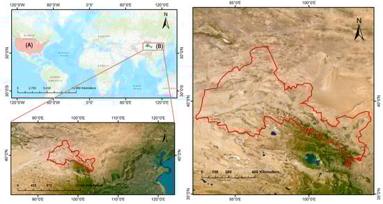
Figure 1.
Study area: location of the source and target domains, where (A) represents the source domain and (B) represents the target domain.
The source domain selected for this study encompasses several major agricultural states in the United States, including Iowa, Missouri, Kansas, Minnesota, North Dakota, and South Dakota. These states, primarily located in the Midwest and Great Plains regions, form the core of U.S. agricultural production. Their agricultural systems are dominated by crops such as maize, soybeans, and wheat. Benefiting from fertile soils, favorable climatic conditions, and high levels of mechanization, these regions provide a rich and diverse data source for transfer learning applications.
2.2. Satellite Imagery and Preprocessing
In crop classification tasks involving significant geographic spatial differences, variations in environmental characteristics, climatic conditions, and data availability between the source and target domains pose challenges for transfer learning. Under such circumstances, relying on a single data source for transfer tasks may struggle to achieve stable classification performance. To address this challenge, the integration of multi-source remote sensing data and dense time series analysis has emerged as a key strategy. The combined use of optical imagery and synthetic aperture radar (SAR) data has been shown to enhance crop mapping accuracy and has been widely adopted [40,41,42,43]. SAR data, with its microwave imaging capabilities, is unaffected by cloud cover and illumination conditions, allowing for continuous surface scattering observations over time and providing a stable data foundation for crop classification in the target region. Meanwhile, the generation of dense time series data, by extracting multi-temporal features, enables a comprehensive characterization of crop phenological dynamics and growth variations [44,45,46]. By leveraging phenological features extracted from dense time series, classifiers can effectively capture crop growth rhythms, developmental stages, and seasonal variations, which is particularly crucial in regions with diverse crop types, such as the Hexi Corridor. Therefore, in this study, input features for the crop mapping task are derived from dense time series data constructed using Sentinel-1, Sentinel-2, and Landsat-8. The spectral bands used are listed in Table A1 in Appendix A.
The Sentinel-1 constellation, comprising Sentinel-1A and Sentinel-1B, is equipped with C-band synthetic aperture radar (SAR) sensors operating at a central frequency of 5.405 GHz. It offers four imaging modes: Interferometric Wide Swath (IW), Extra Wide Swath (EW), Strip Map (SM), and Wave (WV) [47]. This study uses the S1_GRD dataset, preprocessed with the Sentinel-1 Toolbox on Google Earth Engine (GEE), which includes thermal noise removal, radiometric calibration, and orthorectification. The data were then clipped to the study area using GEE, with the primary dataset consisting of dual-polarization (VV + VH) data in IW mode. Sentinel-1 data can be downloaded from https://dataspace.copernicus.eu/ (accessed on 15 August 2024).
The Sentinel-2 constellation consists of Sentinel-2A and Sentinel-2B, operating in push-broom imaging mode with a 290 km swath width. Its Multi-Spectral Imager (MSI) captures 13 spectral bands at 10 m, 20 m, and 60 m resolutions, with a 5-day revisit time [48]. Data are available at https://dataspace.copernicus.eu/ (accessed on 13 August 2024). Landsat-8, launched by the United States Geological Survey (USGS) and the National Aeronautics and Space Administration (NASA), features 11 spectral bands and a 16-day revisit cycle, supporting land use classification, environmental monitoring, and disaster response [49]. Data can be accessed at https://earthexplorer.usgs.gov/ (accessed on Day 13 August 2024).
For this study, Sentinel-1, Sentinel-2, and Landsat-8 imagery from the entire year of 2022 (1 January 2022–31 December 2022) was selected. Cloud removal was performed for Sentinel-2 and Landsat-8 imagery using the QA60 band for Sentinel-2 and the QA band for Landsat-8, with missing values due to cloud removal interpolated using linear interpolation. To generate time-series imagery, Sentinel-2 imagery was processed using a maximum-value composite at a weekly scale, while Sentinel-1 and Landsat-8 imagery were composited at a monthly maximum-value scale.
2.3. Sample Data
For the mapping task, we selected five crop types in both the source and target domains: maize, alfalfa, oats, rapeseed, and spring wheat. The spatial distribution, quantity, and proportion of the samples are shown in Figure 2 and Table 1.
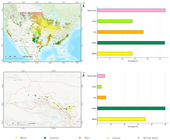
Figure 2.
Spatial distribution of samples in the source and target domains and the percentage of each type of crop samples in the two domains, respectively.

Table 1.
Crop types and number of labels in two datasets.
2.3.1. CDL-Based Sample Data
CDL is a land cover dataset published by the National Agricultural Statistics Service (NASS), the United States Department of Agriculture (USDA). It is primarily used for monitoring and assessing cropland area and crop planting conditions across the United States and has been widely applied in agricultural monitoring, land management, and environmental research [50,51,52]. CDL is generated using remote sensing techniques, integrating satellite imagery and ground survey data. With a spatial resolution of 30 m, it provides a high level of detail, making it valuable for analyzing crop trends, assessing agricultural productivity, and supporting food security monitoring. The dataset classifies various land cover types, with a primary focus on cropland categories (e.g., maize, soybeans, wheat, and alfalfa) as well as non-cropland categories (e.g., forests and wetlands). Each pixel in the dataset is assigned a confidence value ranging from 0 to 100%, indicating the classification certainty. The CDL dataset is updated annually, and for this study, the 2022 CDL data were obtained via the GEE platform.
In this study, the 2022 CDL dataset was used as the source domain data for transfer learning. A confidence mask (greater than 95%) was generated to ensure high classification reliability. To reduce sampling errors, patches with fewer than 100 pixels were removed. Training sample datasets were then constructed by randomly generating points and validating them through visual interpretation.
2.3.2. Ground Truth Data
The ground truth data used in this study comprise crop-type samples collected in 2022 within the Hexi Corridor. These samples are distributed across both smallholder farmlands and large-scale consolidated farmlands, covering a diverse range of plot types. Given that the highest spatial resolution of the satellite imagery used in this study is 10 m, specific considerations were made during the field survey to ensure the reliability of the collected samples. To maintain sufficient 10 × 10 m pixel coverage within each plot, we prioritized marking regularly shaped fields and avoided long and narrow plots whenever possible. This approach was adopted to ensure that the collected samples accurately represent the crop types and minimize potential classification errors.
After completing the field data collection, the samples were imported into the GEE platform for further validation. This process involved comparing the Normalized Difference Vegetation Index (NDVI) phenological curves to verify sample consistency. Additionally, any samples affected by cloud cover were discarded to ensure that only valid and accurate samples were retained for analysis.
Specifically, since the final prediction locations in this study are all within the target domain (Hexi Corridor), we extracted 30% of the ground truth data as an independent test set. The accuracy evaluation of each crop classification mapping model in this paper is conducted based on this independent test set.
2.4. Methodology
The workflow of this study is shown in Figure 3. To evaluate whether transfer learning based on CDL data can improve crop type identification in the Hexi region, we designed two experimental setups as shown in Table 2. The models mentioned in the table will be described in detail in Section 2.4.3. Each model differs in terms of the data used, training stages, and classification algorithms. Since the final objective of all models is crop classification in the target domain, we allocated 30% of the crop samples collected from the Hexi region as an independent test set to evaluate classification accuracy. The remaining 70% of the target domain data were incrementally introduced during Stage B to assess the impact of adding target domain samples. Given the limited availability of target domain data, we allocated 20% of the target domain dataset as a validation set during the transfer process. To ensure training stability, we employed a five-fold cross-validation strategy to assess model performance throughout the training phase.
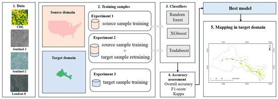
Figure 3.
Workflow of this study.
Table 2.
Experimental setup and characteristics of different models.
2.4.1. Statistical Comparison and Similarity Quantification Between the Two Domains
Transfer learning applies the knowledge learned from solving problems in the source domain to different but related tasks in the target domain. In the field of transfer learning, a prerequisite is that the source and target domains must satisfy either a difference in feature spaces (Xs ≠ Xt) or a difference in marginal probability distributions (P(Xs) ≠ P(Xt)) [23]. For transfer learning in the crop mapping task, the feature spaces of two regions should be identical, while the feature representations of the samples (i.e., feature pairs) or the marginal probability distributions should exhibit a low level of similarity. To validate the feasibility of transfer learning before training the model, this study employs the Kolmogorov–Smirnov (K-S) test to assess the differences in the probability distributions between the source and target domain sample inputs. The Kolmogorov–Smirnov (K-S) test is a non-parametric statistical method commonly used to evaluate whether sample data fits a theoretical distribution or to compare whether two samples come from the same distribution [53]. The test is based on comparing the difference between the empirical distribution function (EDF) of the sample and the theoretical distribution or the EDF of another sample. The test statistic D is calculated as follows:
where Fm and Gn represent two empirical distribution functions of the two samples of size m and n, respectively, and sup is for the supremum function. The null hypothesis states that both samples have the same underlying distribution, and it is rejected if the p-value of the test is less than the level of significance, which was set for all tests at 0.05.
Dynamic Time Warping (DTW) is a method used to measure the similarity between time series by aligning them in a way that minimizes the cumulative distance between corresponding points [54]. It is particularly useful for handling time series with varying lengths and time scales. In remote sensing, DTW is applied to compare NDVI time series between source and target domains, quantifying the similarity in crop phenology. This approach enables effective knowledge transfer by assessing temporal similarities in crop growth cycles across regions.
NDVI is a commonly used vegetation index for monitoring plant growth conditions through remote sensing. It measures vegetation density and health by analyzing the reflection difference between the red and near-infrared bands in remote sensing imagery [55]. The NDVI time series is closely linked to crop phenology, as the changes in NDVI throughout the growing season can reveal critical phenological stages of crops, such as planting, flowering, and maturation periods. In this study, NDVI was used as a feature to generate time series for the same crop in both regions, which represents the phenology of the same crop across different regions.
2.4.2. Input Features
Differences in crop phenology provide valuable information for crop mapping, and satellite images with time series can effectively capture these phenological characteristics. Vegetation indices are commonly used to qualitatively assess vegetation coverage and vigor [56]. In agricultural applications, they are commonly applied in crop type identification, crop growth monitoring, and related tasks. In this study, we used 16 vegetation indices as features, as shown in Table A2, calculated from the Sentinel-2 and Landsat-8 bands. Additionally, all bands from Sentinel-2 and Landsat-8, along with the VV and VH polarization modes from Sentinel-1, were utilized as input features.
2.4.3. Classifiers and Parameter Settings
We selected several machine learning algorithms, including Random Forest, XGBoost, and TrAdaBoost, as strategies for the transfer-learning-based crop classification task.
Random Forest is a classic machine learning algorithm based on bootstrap aggregation (bagging), consisting of multiple decision trees. Each tree is trained on a bootstrapped dataset, and classification is determined by majority voting [57]. Due to its robustness to noise, high-dimensional data handling, and feature importance ranking, Random Forest is widely used in remote sensing analysis and crop classification [58,59,60].
XGboost is a gradient boosting decision tree (GBDT)-based algorithm designed for efficient and scalable structured data processing [61]. It optimizes loss functions through feature splitting and sequential tree building, with L1 and L2 regularization to prevent overfitting. Supporting parallel computing and distributed processing, XGBoost is extensively used in classification, regression, and ranking tasks, excelling in data mining and machine learning competitions.
Both XGBoost and Random Forest were employed to support incremental training for transfer learning. The modified versions of these algorithms for transfer learning are referred to as RFtransfer and XGBoosttransfer in this study, respectively. The base models for both algorithms, referred to as RFnaive and XGBoostnaive, were trained using the source domain dataset. Specifically, the RFnaive model was set with n_estimators = 200 and max_depth = 10.
In RFtransfer, we set warm_start = True, allowing the model to retain the tree structure learned from the source domain and gradually add new trees to adapt to the data distribution in the target domain. For retraining with the target domain data, we adopted a progressive strategy: during the first half of the fine-tuning process (Rounds 1–5), 5 trees were added per round, while in the latter half (Rounds 6–10), 10 trees were added per round. This approach is based on the assumption that the gradual incorporation of target domain data can enhance model performance as more target data becomes available. In XGBoosttransfer, we utilized the xgb_model parameter to load the model trained on the source domain and performed incremental learning by continuing to add new trees to the existing model structure. Specifically, we set num_boost_round = 10,000 and implemented early stopping with a patience of 50 rounds. This strategy not only effectively inherits the model structure and knowledge from the source domain but also enhances adaptability to the target domain’s feature distribution, thus achieving fine-tuning under the framework of transfer learning.
TrAdaBoost is a sample reweighting-based transfer learning algorithm designed to improve classification accuracy in the target domain by assigning different weights to source and target domain samples [62]. In each iteration, TrAdaBoost trains an initial classifier using source domain samples and calculates the classification error. Based on this error, the algorithm adjusts sample weights, gradually reducing the weights of misclassified source domain samples while increasing the weights of target domain samples. This mechanism effectively transfers knowledge from the source to the target domain while mitigating negative transfer effects caused by distribution discrepancies.
The efficacy of TrAdaBoost relies on harmonizing instance reweighting with base learner biases. To identify the most suitable base learners, we tested TrAdaBoost with various classifiers, including SVM, RF, DT, and LightGBM. Based on their superior performance, Random Forest and Decision Tree were chosen, leading to the development of two TrAdaBoost variants: TrAdaBoost_RF and TrAdaBoost_DT. TrAdaBoost_RF integrates ensemble randomization with adaptive instance weighting, effectively mitigating domain-specific biases through stochastic feature selection and data sampling. Its dual randomization enhances cross-domain feature stability, ensuring robust crop identification across diverse environmental conditions and sensor variations. TrAdaBoost_DT captures the complex features of crops through deep decision trees, while adaptively reweighting sample weights to improve classification performance across different regions. At the same time, to compare the effectiveness of TrAdaBoost, we also set up RFnaive and DTnaive, which refer to the basic RF model and DT model trained solely with source domain data.
In this study, the input for the TrAdaBoost algorithm includes training samples from the source domain (Ts) and the target domain (Tt), a base classifier, and the maximum number of iterations (N).
The following section presents the detailed TrAdaBoost implementation process, developed using the Python 3.9 programming environment and the adapt library (version 0.1.0):
- 1.
- Normalize weights:
- 2.
- Fit an estimator on source and target labeled data with the respective importance weights:
- 3.
- Compute error vectors of training instances:
- 4.
- Compute the total weighted error of target instances:
- 5.
- Update source and target weights:
- where
- 6.
- Return to step 1 and loop until the number N of boosting iterations is reached.
The predictions are then given by the vote of the last computed estimators, weighted by their respective parameter .
For the TrAdaBoost algorithm, the number of iterations is set to n_estimators = 30. Considering factors such as the training data volume and time, the base classifier RF is set with n_estimators = 80 and max_depth = 7. For the base classifier DT, max_depth is set to 5, with all other parameters left at their default values. The Python version used in this study is 3.9.
Finally, we also set up two models, RFlocal and DTlocal, for comparison (Experiment 3). These models are trained solely using the target domain data with Random Forest and Decision Tree, respectively, and are used to compare with other transfer models to verify the effectiveness of transfer learning.
2.4.4. Accuracy Evaluation
The confusion matrix is commonly used in image accuracy evaluation, primarily to compare classification results with the actual observed values. It displays the accuracy of the classification results in an (n × n) matrix. In this study, we evaluate the performance of classification algorithms by constructing confusion matrices. The evaluation metrics include overall accuracy (OA), recall, class mean recall, precision, the Kappa coefficient, as well as F1-score, macro F1-score, and weighted F1-score.
3. Results
3.1. Domain Difference
The p-values calculated using the K-S test are all less than 0.05. This statistically indicates a significant difference between the two domains. Such substantial differences may stem from variations in farming practices, climatic characteristics, and field management methods between the two regions.
As shown in Figure 4, which compares the NDVI curves between the source and target domains, maize exhibits a high degree of phenological similarity across the two domains. Specifically, during the greening period (weeks 20–25), both the source and target domains show a sharp increase in NDVI, with the NDVI reaching its peak around week 30. While other crops demonstrate similar phenological trends, some temporal shifts are observed. To further evaluate the phenological similarity between the two domains, we employed DTW to calculate the distance between the NDVI time series of the same crop in the source and target domains. Table 3 summarizes the DTW-based distance results. The results show that there are acceptable morphological differences in the NDVI time series curves of the same crop between the source and target domains, indicating that transfer learning is suitable for adjustment and adaptation.
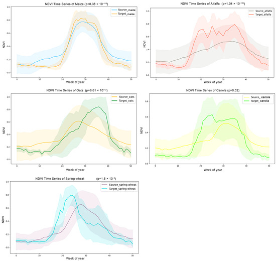
Figure 4.
Averaged NDVI weekly time series for each crop type for source domain and target domain, with x-axis representing image compose dates and y-axis representing vegetation index value.
Table 3.
DTW-based distances between crop phenology curves in the source and target domains.
The observed similarity in trends between crops in the source and target domains, coupled with differences in specific time points, can be attributed to the fact that crops at similar latitudes tend to exhibit similar phenological patterns. However, due to variations in climate, elevation, and planting environments between the two domains, phenological shifts such as earlier or later growth stages may occur even for the same crop species. For instance, the southern part of the Hexi Corridor, located near the Qilian Mountains, has a higher elevation and lower temperatures, resulting in insufficient thermal accumulation and a shorter growing season for crops planted in that region. In summary, while there are both similarities and statistically significant differences between the two domains, this provides strong support for the applicability of transfer learning in crop identification across these two regions.
3.2. Comparison of the Performance of Different Transfer Strategies
Table 4 presents the performance of the respective algorithms in Experiments 1, 2, and 3 on the target domain test set. In Experiment 1, among the original models, XGBoostnaive achieved the best performance with an accuracy of 0.7833 and a Kappa coefficient of 60.09%, followed by RFnaive, while DTnaive showed the poorest performance. Experiment 2 demonstrated that RFtransfer was the most effective transfer learning model in this study, reaching an accuracy of 92.26% and a Kappa coefficient of 0.8723. It was followed by TrAdaBoost_RF, XGBoosttransfer, and TrAdaBoost_DT, with all transfer models achieving accuracies above 90%. Experiment 3 served as a comparison for transfer learning, where models were trained solely on target domain data. The RFlocal model achieved an accuracy of 89.90% and a Kappa coefficient of 0.8399. In Experiment 2, all models adjusted using target domain data outperformed the local model, validating the effectiveness of transfer learning.
Table 4.
The performance of different algorithms in Experiments 1, 2, and 3.
The weighted F1-scores of specific crops in Experiment 2 are presented in Table 5. In terms of the specific crop F1-scores, XGBoosttransfer achieves the highest F1-score for maize, while RFtransfer performs the best in F1-score for the other crops.
Table 5.
Weighted F1-scores of different crops under various transfer learning algorithms in Experiment 2.
The performance of the models in Experiment 2 and Experiment 3 is shown in Figure 5. The vertical axis represents the overall accuracy, while the horizontal axis indicates the percentage of target domain data accumulated for training. It can be observed that the transfer learning strategy employed in Experiment 2 effectively improved the classification accuracy. As the amount of incorporated target domain data increased, the model accuracies exhibited a clear upward trend.

Figure 5.
Overall accuracy of models in Experiment 2 and Experiment 3 on the test set with increasing amounts of target domain data.
Specifically, the overall accuracy of RFtransfer increased from 87.93% to 92.26%, XGBoosttransfer improved from 85.43% to 90.29%, Tradaboost_RF rose from 84.56% to 91.86%, and Tradaboost_DT increased from 77.30% to 90.94%. Similarly, RFlocal and DTlocal also demonstrated a gradual improvement in accuracy with the addition of target domain data, with RFlocal improving from 82.02% to 89.90% and DTlocal increasing from 62.34% to 76.25%. However, their performance remained lower than that of the models utilizing the transfer learning strategy in Experiment 2.
In the classification performance for each crop, Figure 6 shows the performance of the original models as well as the models that incorporate target domain data on the target domain test set. Maize and alfalfa exhibit relatively high F1-scores in the original models, with values of 0.8743 and 0.7618 (RFnaive), 0.8897 and 0.8523 (XGboostnaive), and 0.749 and 0.6175 (DTnaive), respectively, while other crops show relatively lower F1-scores in the original models. As target domain data are incorporated, there is an overall increase in the F1-scores for various crops, with particularly noticeable improvements for oats, canola, and spring wheat. By the final stage, after incorporating the entire target domain training data, the F1-scores for different crops reached above 0.93 for maize and alfalfa, over 0.85 for oats and spring wheat, and the lowest for canola at 0.61.
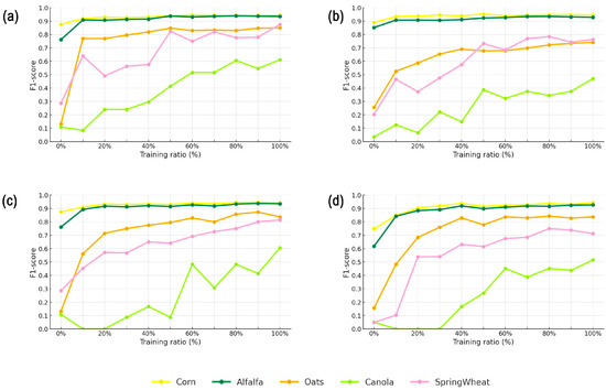
Figure 6.
The performance of each crop under different transfer strategies: (a) represents RFtransfer, (b) represents XGboosttransfer, (c) represents Tradaboost_RF, and (d) represents Tradaboost_DT.
The confusion matrix reveals the specific misclassification patterns of crop categories, as shown in Figure 7. The rows from the first to the fourth represent the four transfer learning algorithms, and from left to right, the matrices display the confusion results when 0%, 10%, 50%, and 100% of the target domain data are used for transfer. These represent the beginning, middle, and end stages of incorporating target domain data. From Figure 7, it can be observed that when only source domain data are used for training, maize and alfalfa show higher accuracy, while other crops are poorly classified, resulting in significant misclassification. When 10% of the target domain data are added for retraining, the misclassification between oats and canola is resolved, and the classification accuracy for oats begins to improve. However, canola and spring wheat are still mainly misclassified as major crops (such as alfalfa and maize). As more target domain data are gradually incorporated (50–100%), this misclassification is notably corrected, leading to improvements in the classification accuracy of both canola and spring wheat.
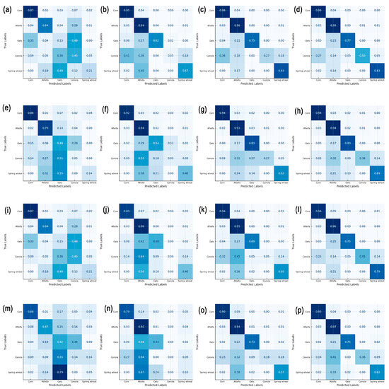
Figure 7.
(a–d) represent RF models using 0%, 10%, 50%, and 100% of the target domain data, respectively; (e–h) represent XGBoost models using 0%, 10%, 50%, and 100% of the target domain data, respectively; (i–l) represent TrAdaBoost_RF models using 0%, 10%, 50%, and 100% of the target domain data, respectively; (m–p) represent TrAdaBoost_DT models using 0%, 10%, 50%, and 100% of the target domain data, respectively.
3.3. Feature Importance Ranking of the Optimal Transfer Model
To investigate the contribution of multi-source data integration to model stability, we conducted a feature importance ranking based on the input features of the optimal transfer learning algorithm, RFtransfer. Among the top 200 most important features, 191 originated from Sentinel-2, 7 from Landsat-8, and only 2 from Sentinel-1. Additionally, the top 30 features and their importance rankings are illustrated in Figure 8. The naming convention for the features on the y-axis in the figure follows the format “SatelliteData_Index/Band_TimeStep”. For example, the top three features in terms of importance are VGCI, kNDVI, and NDVI, all calculated from Sentinel-2 satellite data as maximum composites for Week 17.
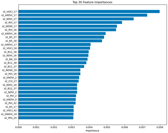
Figure 8.
Top 30 feature importance rankings of the RFtransfer model.
These results indicate that Sentinel-2 data contributed most significantly to model performance in the crop classification task under the transfer learning framework. Benefiting from its high spectral and temporal resolution, the Sentinel-2 time series more effectively captured crop spectral responses and phenological dynamics, thus playing a dominant role in the model. In contrast, the Landsat-8 time series, with its lower temporal resolution, offered less timely features and contributed less to the classification results. The backscatter information provided by Sentinel-1 radar data showed limited sensitivity in distinguishing between crop types, resulting in a relatively low feature importance in the model.
3.4. Crops Cultivated Areas Identification in Hexi
Since RFtransfer exhibited the best performance among all transfer learning algorithms, we selected the RFtransfer model adjusted with the full target domain data to generate the crop type map for the Hexi Corridor in 2022. It is worth noting that the trained model was applied within the cropland mask area of the Hexi Corridor.
Due to the limited number of test set samples, the accuracy reported above may not fully reflect the classification performance across the entire study area. Therefore, we further evaluated the accuracy of crop mapping by incorporating statistical data and datasets such as the 2001–2023 China Corn Planting Distribution Dataset (CCD-Maize) [63]. To estimate the mapped crop areas, we calculated the number of pixels classified as each crop type in each city within the Hexi region, then multiplied it by the pixel size (10 m × 10 m) to obtain the estimated crop area. The resulting mapped areas for maize, alfalfa, oats, canola, and spring wheat in the Hexi region were 55.19, 33.89, 5.84, 37.53, and 11.76 million hectares (MHs), respectively.
Additionally, we referenced statistical yearbooks for reported maize and wheat planting areas, aggregating them at the city level in the Hexi region for comparison, as shown in Figure 9. The mapped maize planting area exhibited high consistency with the statistical data, whereas discrepancies were observed in the wheat planting areas in Jiuquan and Jinchang. This difference may be attributed to the fact that statistical data for wheat in this region include both spring wheat and winter wheat, leading to variations in the comparison.
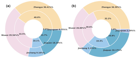
Figure 9.
The proportion of maize (a) and spring wheat (b) planting areas in each city. The outer ring represents the results obtained using RFtransfer, while the inner ring represents the city-level statistical data.
Additionally, we compared the classification results of this study with the 2001–2023 China Crop Dataset–Maize (CCD-Maize) [64] (Figure 10). Compared to these datasets, our study produced higher-resolution results with more complete field boundaries at a finer spatial scale. In the Hexi region, maize, alfalfa, and spring wheat are distributed across all five cities, with maize having the largest planting area, making it the dominant crop in the region. In contrast, oats and canola are primarily concentrated in higher-altitude areas.
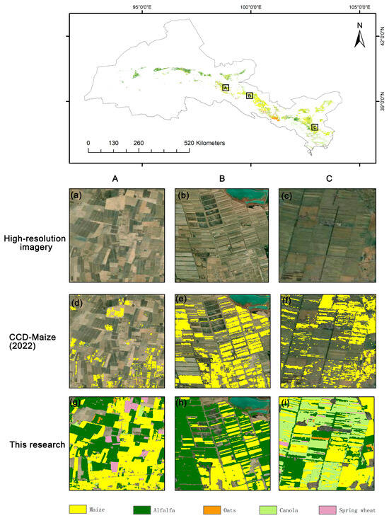
Figure 10.
The crop mapping results based on the RFtransfer model are compared with high-resolution imagery and the CCD-Maize dataset. A, B, and C represent the three typical regions we selected. (a–c) show high-resolution imagery, (d–f) present the CCD-Maize dataset, and (g–i) illustrate the crop mapping results based on the RFtransfer model.
4. Discussion
4.1. The Advantages of Transfer Learning
In classification tasks based on machine learning and remote sensing imagery, the focus is often on traditional machine learning and deep learning methods, which typically require a sufficient quantity and quality of training samples to ensure adequate classification accuracy. However, sample collection is a labor-intensive process, and sample scarcity is a common issue. Transfer learning has emerged as a promising strategy to address these challenges. Many studies have employed transfer learning methods such as fine-tuning-based transfer learning (FT), few-shot learning (FSL), multi-task learning (MSL), and unsupervised domain adaptation (UDA) to tackle the problem of sample scarcity [26]. For crop mapping across geographic regions, challenges remain in terms of model generalization due to differences in geographic space and crop phenology, making large-scale, cross-regional crop mapping difficult. Prior knowledge and reference data can play a crucial role in transfer learning for crop mapping [64,65]. Transfer learning can enable cross-temporal and cross-spatial crop mapping by transferring samples or models, applying existing sample datasets to other regions, and providing solutions for regions with limited sample availability [66].
Despite statistical and climatic differences between regions, transferring crop classification model knowledge across geographic areas is still feasible. In the context of limited and imbalanced target domain sample data, this study adopted a transfer learning strategy. Specifically, by localizing the model with labeled data from the target domain on top of a source domain model, the use of the transfer learning strategy significantly reduced the cost of label acquisition in the target domain. The results indicate an improvement in classification accuracy for the adjusted model, demonstrating that even with discrepancies in crop sample data phenology, distribution, and quantity between the source and target domains, transfer learning can still transfer knowledge from the source domain to the target domain. In this study, using data from the Hexi Corridor improved model accuracy, suggesting that the model can learn unique crop features from the target domain, thereby enhancing model robustness and generalization. This provides a valuable reference for crop type mapping in the Hexi Corridor.
4.2. The Effectiveness of the Transfer Learning Strategy in Hexi Corridor
In this study, the classification performance of staple crops was significantly better than that of minor crops. Even without retraining the model with target domain data, the model trained only on source domain data performed well in classifying staple crops. The classification accuracy of maize and alfalfa reached 0.89 and 0.85, respectively, in the XGboosttransfer model, indicating that the feature distribution of staple crops in the target domain is highly similar to that in the source domain, which enhances the model’s generalization ability. This further suggests that even when data from the target region is scarce or unavailable, crop mapping in the local area can still benefit from models trained on source domain data. However, the classification performance of minor crops, such as oats, canola, and spring wheat, is relatively poor, with lower classification accuracy. This may be related to factors such as differences in crop phenological characteristics and distribution shifts between the source and target domains. In particular, the Hexi Corridor is located on the northeastern edge of the Qinghai–Tibet Plateau, an area with some high-altitude regions. Due to its unique geographical location, crop phenology in this area is delayed. Additionally, the relatively small sample size of minor crops in the target domain limits the model’s learning ability for these categories. The imbalanced distribution of sample classes causes the classification model to overfit the dominant classes’ feature distributions, which is common in imbalanced data. This finding is similar to the results of Arias, where crop mapping using imbalanced datasets showed better classification performance for the dominant sample types [67].
At the same time, Experimental results indicate that as the number of labeled target domain samples gradually increases during retraining, the model’s classification performance improves, and the more target domain data available, the better the classification results. This trend is consistent with the findings of Miloš Pandžić, which demonstrate that transfer learning methods incorporating target domain data are versatile and effective in crop classification tasks [13]. Compared to large-scale crop-type products, this study produced crop-type distribution maps with a finer scale, covering a smaller area but with higher accuracy, better spatial resolution, and multiple crop types. This provides an actionable reference for regions with high fragmentation of cultivated land, complex crop planting types, and a lack of sufficient samples, making accurate crop mapping in sample-scarce areas feasible.
4.3. Comparison of Transfer Learning Algorithms
Aiming to train an initial model with strong generalization capability, the source domain data used in this study was widely distributed and balanced across different crop types, incorporating samples from various climatic conditions and phenological stages. Based on this, we applied transfer learning using the RF, XGBoost, and TrAdaBoost algorithms. After retraining with target domain data, the RFtransfer model achieved the highest classification accuracy, followed by TrAdaBoost_RF, with all transfer models reaching accuracies above 0.90.
However, under these conditions, TrAdaBoost did not demonstrate the best performance. One possible reason lies in its sensitivity to class imbalance and the limited size of target domain samples. Its effectiveness relies heavily on several hyperparameters, such as the number of iterations, initial weights, and the performance of weak classifiers. Without careful tuning, TrAdaBoost may suffer from poor convergence. In contrast, RF and XGBoost exhibit greater robustness when dealing with imbalanced samples and domain distribution shifts. They offer more stable performance and are easier to deploy, making them well suited for practical applications in sample-scarce scenarios. In addition, the wide spatial distribution of the source domain samples (e.g., including both southern and northern U.S. regions) may have introduced considerable intra-class phenological variability. Such internal heterogeneity can make it difficult for TrAdaBoost to accurately distinguish between source samples that are similar or dissimilar to the target domain during early training stages. This may affect its weight adjustment process and weaken its theoretical advantage. In contrast, the RF and XGBoost models, trained on the combined source and target datasets, are better able to learn consistent patterns from the overall data and thus exhibit stronger generalization capabilities.
These findings suggest that the optimal application scenarios for different transfer learning algorithms may vary depending on data characteristics. In future work, selecting source domain samples with phenological profiles more closely aligned with those of the target domain may help reduce sample interference and improve the performance of TrAdaBoost.
4.4. Uncertainty and Potential Refinement
Since the performance of classification models largely depends on the training and test samples, there are inherent differences in various studies not only in the categories, data volumes, and distributions of training and test datasets, but also in the choice of crop types, geographical location of transfer, selected evaluation metrics, and other related parameters. Therefore, systematically comparing the results with other crop classification studies is challenging [13,35]. Facing the challenges of evaluation, we have assessed the performance using an independent test set and by comparing it with statistical data. In this study, due to the imbalanced data distribution in the target domain, traditional local training methods are not applicable. This is because the sample sizes of some crop categories in the target domain are too small to support the training of local classifiers. Therefore, this study does not include a comparison with local data training in the target domain. From the perspective of comparison with local training, while transfer learning demonstrates significant capabilities, it should not be applied unconditionally. For regions that lack or have poor quality in situ data, transfer learning can effectively solve the challenges of crop mapping in those areas. However, when a certain amount of high-quality target domain data is available, transfer learning may not necessarily outperform traditional local training-based crop identification methods [17]. Some studies have pointed out that traditional local training methods require hyperparameter optimization before model training, while transfer learning only requires model retraining, which may lead to substantial differences in processing time [13]. Through this study, we explored the feasibility of using transfer learning strategies for crop type mapping in the Hexi Corridor. The research shows that transfer learning can effectively transfer knowledge learned from the source domain to the target domain, thereby reducing the cost of labeling target domain samples to some extent. Overall, transfer learning provides a solution to the problem of insufficient target domain data while also reducing the time required for training the model from scratch, thus improving mapping efficiency. This provides valuable references for future research on crop classification in regions with limited data.
Considering the presence of interannual climatic variability and other unstable factors, it is also crucial to evaluate the adaptability and robustness of transfer learning models across different years. To this end, the RFtransfer model trained exclusively on 2022 data was independently validated using the 2023 dataset, in order to assess its crop type prediction performance under varying climatic conditions. The detailed validation results are provided in the Supplementary Materials. Although this study successfully implemented crop mapping in the Hexi Corridor using a transfer learning strategy, reducing the cost of local sample annotation, certain uncertainties and limitations remain, providing deeper exploration directions for future research. First, transferability estimation remains an important area of investigation. Transferability estimation is used to evaluate the compatibility between datasets and models to ensure the success of transfer learning tasks [68]. The distributional differences between the source and target domains pose challenges to transfer learning, especially in instance-based transfer. In a study by Wang, growing degree days (GDD) were used to quantify regional differences, and the results showed a correlation between GDD differences and model transfer accuracy [29]. Therefore, before applying crop classification using transfer learning to other regions, it is necessary to conduct transferability estimation. Second, the expansion of methods and improvements in transfer learning strategies are also key future directions. This study mainly employed shallow machine learning methods, but future research could explore alternative transfer learning strategies, such as deep learning-based transfer learning, including techniques like model parameter freezing and shared feature extraction layers. Unlike machine learning methods that rely on manually designed features, deep learning approaches offer stronger feature representation capabilities, enabling automatic extraction of spatiotemporal features and reducing dependence on feature engineering. Deep transfer learning can further improve classification performance by leveraging large-scale pretraining and fine-tuning with limited target domain data [7]. Many studies have achieved cross-regional model transfer by employing pretraining on source domain data followed by fine-tuning with target domain data [24,30,35,69], which provides valuable insights into cross-regional crop type recognition using transfer learning. Additionally, spatial resolution limitations represent a key constraint in this study. In regions with highly fragmented farmland, the 10 m resolution Sentinel-2 imagery used in this study may not be sufficient to capture the fine boundaries of small land parcels. High-resolution imagery can better delineate small field boundaries and capture subtle land cover variations, especially in regions with diverse and complex crop types. Future studies could incorporate higher-resolution remote sensing data, such as PlanetScope imagery or WorldView imagery, to improve the spatial resolution of classification and enhance boundary detection accuracy.
5. Conclusions
In this study, high-density time series from Sentinel-2, Sentinel-1, and Landsat-8 imagery were used, and based on RF, XGBoost, and TrAdaBoost algorithms, the effectiveness of instance-based transfer strategies for crop mapping tasks was explored and evaluated in the Hexi Corridor. The results show that under conditions with abundant source domain data and limited target domain data, the transfer strategy performed well, especially for staple crops with large planting areas in the target domain. Even without using target domain data for training, the classification accuracy achieved was quite substantial, with the overall classification accuracy reaching up to 73.88%. The optimal classification accuracy for maize and alfalfa was 88.97% and 85.23%, respectively. During the process of gradually incorporating target domain data, the total accuracy for all models ranged from 0.77 to 0.92, and the F1-score ranged from 0.76 to 0.92. As the proportion of target domain data increased, model accuracy improved. After all target domain data were added, the classification accuracies for RFtransfer, XGBoosttransfer, TrAdaBoost_RF, and TrAdaBoost_DT were 92.26%, 90.29%, 91.86%, and 90.94%, respectively. The best transfer model was RFtransfer. These results demonstrate the effectiveness of the transfer strategy and provide a reference for crop mapping in areas with limited samples.
Supplementary Materials
The following supporting information can be downloaded at: https://www.mdpi.com/article/10.3390/rs17091494/s1, Table S1: Validation results of the RFtransfer model, trained with all target domain data, on the 2023 independent validation dataset; Table S2: Validation results of RFtransfer models progressively trained with increasing target domain data, evaluated on the 2023 independent validation dataset.
Author Contributions
Conceptualization, J.M., S.F. and Q.F.; methodology, J.M.; software, S.F.; validation, J.M.; formal analysis, J.M.; investigation, J.M. and R.Z.; resources, J.M. and R.Z.; data curation, J.M. and S.F.; writing—original draft preparation, J.M.; writing—review and editing, J.M., Q.F., R.W. and S.Z.; visualization, J.M.; supervision, Q.F.; project administration, Q.F. and T.L.; funding acquisition, Q.F. and T.L. All authors have read and agreed to the published version of the manuscript.
Funding
This research was funded by the earmarked fund for China Forage and Grass Research System (CARS-34).
Data Availability Statement
The dataset is available on request from the authors.
Conflicts of Interest
The authors declare no conflicts of interest.
Appendix A
Table A1.
Bands used in this research.
Table A1.
Bands used in this research.
| Satellite | Band | Resolution (m) | Central Wavelength (nm) | Bandwidth (nm) | Description |
|---|---|---|---|---|---|
| Sentinel-1 | C-band | 5–40 | 3.1 (cm) | 1500 (MHz) | Synthetic Aperture Radar (SAR) |
| Sentinel-2 | B1 | 60 | 443 | 20 | Coastal aerosol |
| Sentinel-2 | B2 | 10 | 490 | 65 | Blue |
| Sentinel-2 | B3 | 10 | 560 | 35 | Green |
| Sentinel-2 | B4 | 10 | 665 | 30 | Red |
| Sentinel-2 | B5 | 20 | 705 | 15 | Vegetation Red Edge |
| Sentinel-2 | B6 | 20 | 740 | 15 | Vegetation Red Edge |
| Sentinel-2 | B7 | 20 | 783 | 20 | Vegetation Red Edge |
| Sentinel-2 | B8 | 10 | 842 | 115 | Near Infrared (NIR) |
| Sentinel-2 | B8A | 20 | 865 | 20 | Narrow Near Infrared (NIR) |
| Sentinel-2 | B9 | 60 | 945 | 20 | Water Vapour |
| Sentinel-2 | B10 | 60 | 1375 | 30 | SWIR (Short Wave Infrared) |
| Sentinel-2 | B11 | 20 | 1610 | 90 | SWIR (Short Wave Infrared) |
| Sentinel-2 | B12 | 20 | 2190 | 180 | SWIR (Short Wave Infrared) |
| Landsat-8 | B1 | 30 | 433 | 16 | Coastal Aerosol |
| Landsat-8 | B2 | 30 | 452 | 37 | Blue |
| Landsat-8 | B3 | 30 | 523 | 69 | Green |
| Landsat-8 | B4 | 30 | 695 | 60 | Red |
| Landsat-8 | B5 | 30 | 865 | 60 | Near Infrared (NIR) |
| Landsat-8 | B6 | 30 | 1069 | 190 | Shortwave Infrared (SWIR) |
| Landsat-8 | B7 | 30 | 2201 | 190 | Shortwave Infrared (SWIR) |
| Landsat-8 | B8 | 30 | 482 | 26 | Panchromatic |
| Landsat-8 | B9 | 30 | 1366 | 100 | Cirrus Cloud |
| Landsat-8 | B10 | 100 | 1050 | 300 | Thermal Infrared (TIRS) |
| Landsat-8 | B11 | 100 | 1230 | 300 | Thermal Infrared (TIRS) |
| Landsat-8 | BQA | 30 | Quality Assessment (QA) |
Table A2.
Vegetation index used in this research.
Table A2.
Vegetation index used in this research.
| Index | Formula | Description |
|---|---|---|
| NDVI | (NIR − Red)/(NIR + Red) | Normalized Difference Vegetation Index, a classic measure of vegetation health |
| EVI | 2.5 × (NIR − Red)/(NIR +6 × Red − 7.5 × Blue + 1) | Enhanced Vegetation Index, less sensitive to atmospheric effects and soil background |
| SAVI | (NIR − Red) × (1 + L)/(NIR + Red + L) | Soil Adjusted Vegetation Index, accounts for soil influences in sparse vegetation areas |
| NDRE | (WIR − RE1)/(NIR + RE1) | Normalized Difference Red Edge Index, sensitive to changes in leaf chlorophyll content |
| MSI | SWIR1/NIR | Moisture Stress Index detects changes in plant water content |
| GNDVI | (NIR − Green)/(NIR + Green) | Green Normalized Difference Vegetation Index, sensitive to chlorophyll content |
| CVI | NIR × Red/Green2 | Chlorophyll Vegetation Index focuses on the chlorophyll absorption region |
| PSRI | (RE1 − Red)/NIR | Plant Senescence Reflectance index, sensitive to plant senescence |
| KNDVI | tanh(NDVI2) | Kernel NDVl, a non-linear variation of NDVl |
| NIRv | NIR × NDVI | NIR reflectance adjusted using NDVl to enhance vegetation signal |
| NDTI | (SWIR1 − SWIR2)/(SWIR1 + SWIR2) | Normalized Difference Tillage Index may help distinguish tillage patterns |
| RVI | NIR/Red | Ratio Vegetation Index, simple and related to NDVl |
| NDWI | (Green − NIR)/(Green + NIR) | Normalized Difference Water Index, sensitive to plant and soil moisture |
| VGCI | (NIR − Red)/Red | Vegetation Growth Cycle Index reflects the vegetation growth cycle and its changes |
| NDCI | (RE1 − Red)/(RE1 + Red) | Normalized Difference Chlorophyll Index focuses on chlorophyll contents |
| CARI | Red + (2×(RE1 − Red) ×(Green − Red)) | Chlorophyll Absorption Ratio Index minimizes soil background noise |
In the table, the Sentinel-2 bands are mapped as follows: Blue corresponds to B2, Green corresponds to B3, Red corresponds to B4, Red Edge 1 (RE1) corresponds to B5, Near-Infrared (NIR) corresponds to B8, Shortwave Infrared 1 (SWIR1) corresponds to B11, and Shortwave Infrared 2 (SWIR2) corresponds to B12. Similarly, for Landsat-8 bands, Blue corresponds to Band 2, Green corresponds to Band 3, Red corresponds to Band 4, Near-Infrared (NIR) corresponds to Band 5, Shortwave Infrared 1 (SWIR1) corresponds to Band 6, and Shortwave Infrared 2 (SWIR2) corresponds to Band 7.
References
- Singh, B.K.; Delgado-Baquerizo, M.; Egidi, E.; Guirado, E.; Leach, J.E.; Liu, H.; Trivedi, P. Climate Change Impacts on Plant Pathogens, Food Security and Paths Forward. Nat. Rev. Microbiol. 2023, 21, 640–656. [Google Scholar] [CrossRef] [PubMed]
- Chen, Y.; Lu, D.; Moran, E.; Batistella, M.; Dutra, L.V.; Sanches, I.D.; Da Silva, R.F.B.; Huang, J.; Luiz, A.J.B.; De Oliveira, M.A.F. Mapping Croplands, Cropping Patterns, and Crop Types Using MODIS Time-Series Data. Int. J. Appl. Earth Obs. Geoinf. 2018, 69, 133–147. [Google Scholar] [CrossRef]
- Vali, A.; Comai, S.; Matteucci, M. Deep Learning for Land Use and Land Cover Classification Based on Hyperspectral and Multispectral Earth Observation Data: A Review. Remote Sens. 2020, 12, 2495. [Google Scholar] [CrossRef]
- Segarra, J.; Araus, J.L.; Kefauver, S.C. Farming and Earth Observation: Sentinel-2 Data to Estimate within-Field Wheat Grain Yield. Int. J. Appl. Earth Obs. Geoinf. 2022, 107, 102697. [Google Scholar] [CrossRef]
- Salcedo-Sanz, S.; Ghamisi, P.; Piles, M.; Werner, M.; Cuadra, L.; Moreno-Martínez, A.; Izquierdo-Verdiguier, E.; Muñoz-Marí, J.; Mosavi, A.; Camps-Valls, G. Machine Learning Information Fusion in Earth Observation: A Comprehensive Review of Methods, Applications and Data Sources. Inf. Fusion 2020, 63, 256–272. [Google Scholar] [CrossRef]
- Blickensdörfer, L.; Schwieder, M.; Pflugmacher, D.; Nendel, C.; Erasmi, S.; Hostert, P. Mapping of Crop Types and Crop Sequences with Combined Time Series of Sentinel-1, Sentinel-2 and Landsat 8 Data for Germany. Remote Sens. Environ. 2022, 269, 112831. [Google Scholar] [CrossRef]
- Iman, M.; Arabnia, H.R.; Rasheed, K. A Review of Deep Transfer Learning and Recent Advancements. Technologies 2023, 11, 40. [Google Scholar] [CrossRef]
- Arias, M.; Campo-Bescós, M.Á.; Álvarez-Mozos, J. Crop Classification Based on Temporal Signatures of Sentinel-1 Observations over Navarre Province, Spain. Remote Sens. 2020, 12, 278. [Google Scholar] [CrossRef]
- Beriaux, E.; Jago, A.; Lucau-Danila, C.; Planchon, V.; Defourny, P. Sentinel-1 Time Series for Crop Identification in the Framework of the Future CAP Monitoring. Remote Sens. 2021, 13, 2785. [Google Scholar] [CrossRef]
- Schneider, M.; Broszeit, A.; Körner, M. Eurocrops: A Pan-European Dataset for Time Series Crop Type Classification. arXiv 2021, arXiv:2106.08151. [Google Scholar] [CrossRef]
- Turkoglu, M.O.; D’Aronco, S.; Perich, G.; Liebisch, F.; Streit, C.; Schindler, K.; Wegner, J.D. Crop Mapping from Image Time Series: Deep Learning with Multi-Scale Label Hierarchies. Remote Sens. Environ. 2021, 264, 112603. [Google Scholar] [CrossRef]
- Rußwurm, M.; Pelletier, C.; Zollner, M.; Lefèvre, S.; Körner, M. BreizhCrops: A Time Series Dataset for Crop Type Mapping. arXiv 2020, arXiv:1905.11893. [Google Scholar] [CrossRef]
- Pandžić, M.; Pavlović, D.; Matavulj, P.; Brdar, S.; Marko, O.; Crnojević, V.; Kilibarda, M. Interseasonal Transfer Learning for Crop Mapping Using Sentinel-1 Data. Int. J. Appl. Earth Obs. Geoinf. 2024, 128, 103718. [Google Scholar] [CrossRef]
- Rustowicz, R.M.; Cheong, R.; Wang, L.; Ermon, S.; Burke, M.; Lobell, D. Semantic segmentation of crop type in Africa: A novel dataset and analysis of deep learning methods. In Proceedings of the IEEE/cvf Conference on Computer Vision and Pattern Recognition Workshops, Long Beach, CA, USA, 16–17 June 2019; pp. 75–82. [Google Scholar]
- Zhang, C.; Di, L.; Hao, P.; Yang, Z.; Lin, L.; Zhao, H.; Guo, L. Rapid In-Season Mapping of Corn and Soybeans Using Machine-Learned Trusted Pixels from Cropland Data Layer. Int. J. Appl. Earth Obs. Geoinf. 2021, 102, 102374. [Google Scholar] [CrossRef]
- Wang, Y.; Feng, L.; Sun, W.; Zhang, Z.; Zhang, H.; Yang, G.; Meng, X. Exploring the potential of multi-source unsupervised domain adaptation in crop mapping using Sentinel-2 images. GISci. Remote Sens. 2022, 59, 2247–2265. [Google Scholar] [CrossRef]
- Hao, P.; Di, L.; Zhang, C.; Guo, L. Transfer Learning for Crop Classification with Cropland Data Layer Data (CDL) as Training Samples. Sci. Total Environ. 2020, 733, 13869. [Google Scholar] [CrossRef]
- Lin, C.; Zhong, L.; Song, X.-P.; Dong, J.; Lobell, D.B.; Jin, Z. Early- and in-Season Crop Type Mapping without Current-Year Ground Truth: Generating Labels from Historical Information via a Topology-Based Approach. Remote Sens. Environ. 2022, 274, 112994. [Google Scholar] [CrossRef]
- Zhang, W.; Guo, S.; Zhang, P.; Xia, Z.; Zhang, X.; Lin, C.; Tang, P.; Fang, H.; Du, P. A Novel Knowledge-Driven Automated Solution for High-Resolution Cropland Extraction by Cross-Scale Sample Transfer. IEEE Trans. Geosci. Remote Sens. 2023, 61, 4406816. [Google Scholar] [CrossRef]
- Cui, Y.; Yang, G.; Zhou, Y.; Zhao, C.; Pan, Y.; Sun, Q.; Gu, X. AGTML: A Novel Approach to Land Cover Classification by Integrating Automatic Generation of Training Samples and Machine Learning Algorithms on Google Earth Engine. Ecol. Indic. 2023, 154, 110904. [Google Scholar] [CrossRef]
- Wen, Y.; Li, X.; Mu, H.; Zhong, L.; Chen, H.; Zeng, Y.; Miao, S.; Su, W.; Gong, P.; Li, B.; et al. Mapping Corn Dynamics Using Limited but Representative Samples with Adaptive Strategies. ISPRS J. Photogramm. Remote Sens. 2022, 190, 252–266. [Google Scholar] [CrossRef]
- Niu, S.; Liu, Y.; Wang, J.; Song, H. A Decade Survey of Transfer Learning (2010–2020). IEEE Trans. Artif. Intell. 2020, 1, 151–166. [Google Scholar] [CrossRef]
- Yang, Q.; Zhang, Y.; Dai, W.; Pan, S.J. Introduction. In Transfer Learning; Cambridge University Press: Cambridge, UK, 2020; pp. 3–22. [Google Scholar]
- Gadiraju, K.K.; Vatsavai, R.R. Remote Sensing Based Crop Type Classification Via Deep Transfer Learning. IEEE J. Sel. Top. Appl. Earth Obs. Remote Sens. 2023, 16, 4699–4712. [Google Scholar] [CrossRef]
- Nowakowski, A.; Mrziglod, J.; Spiller, D.; Bonifacio, R.; Ferrari, I.; Mathieu, P.P.; Garcia-Herranz, M.; Kim, D. Crop Type Mapping by Using Transfer Learning. Int. J. Appl. Earth Obs. Geoinf. 2021, 98, 102313. [Google Scholar] [CrossRef]
- Ma, Y.; Chen, S.; Ermon, S.; Lobell, D.B. Transfer Learning in Environmental Remote Sensing. Remote Sens. Environ. 2024, 301, 113924. [Google Scholar] [CrossRef]
- You, N.; Dong, J. Examining Earliest Identifiable Timing of Crops Using All Available Sentinel 1/2 Imagery and Google Earth Engine. ISPRS J. Photogramm. Remote Sens. 2020, 161, 109–123. [Google Scholar] [CrossRef]
- Lei, L.; Wang, X.; Zhang, L.; Hu, X.; Zhong, Y. CROPUP: Historical Products Are All You Need? An End-to-End Cross-Year Crop Map Updating Framework without the Need for in Situ Samples. Remote Sens. Environ. 2024, 315, 114430. [Google Scholar] [CrossRef]
- Wang, S.; Azzari, G.; Lobell, D.B. Crop Type Mapping without Field-Level Labels: Random Forest Transfer and Unsupervised Clustering Techniques. Remote Sens. Environ. 2019, 222, 303–317. [Google Scholar] [CrossRef]
- Koukos, A.; Jo, H.; Sitokonstantinou, V.; Tsoumas, I.; Kontoes, C.; Lee, W. Towards Global Crop Maps with Transfer Learning. In Proceedings of the IGARSS 2024-2024 IEEE International Geoscience and Remote Sensing Symposium, Athens, Greece, 7–12 July 2024; pp. 1540–1545. [Google Scholar]
- Orynbaikyzy, A.; Gessner, U.; Conrad, C. Spatial Transferability of Random Forest Models for Crop Type Classification Using Sentinel-1 and Sentinel-2. Remote Sens. 2022, 14, 1493. [Google Scholar] [CrossRef]
- Rusňák, T.; Kasanický, T.; Malík, P.; Mojžiš, J.; Zelenka, J.; Sviček, M.; Abrahám, D.; Halabuk, A. Crop Mapping without Labels: Investigating Temporal and Spatial Transferability of Crop Classification Models Using a 5-Year Sentinel-2 Series and Machine Learning. Remote Sens. 2023, 15, 3414. [Google Scholar] [CrossRef]
- Luo, Y.; Zhang, Z.; Zhang, L.; Han, J.; Cao, J.; Zhang, J. Developing High-Resolution Crop Maps for Major Crops in the European Union Based on Transductive Transfer Learning and Limited Ground Data. Remote Sens. 2022, 14, 1809. [Google Scholar] [CrossRef]
- Xun, L.; Zhang, J.; Yao, F.; Cao, D. Improved Identification of Cotton Cultivated Areas by Applying Instance-Based Transfer Learning on the Time Series of MODIS NDVI. Catena 2022, 213, 106130. [Google Scholar] [CrossRef]
- Antonijević, O.; Jelić, S.; Bajat, B.; Kilibarda, M. Transfer Learning Approach Based on Satellite Image Time Series for the Crop Classification Problem. J. Big Data 2023, 10, 54. [Google Scholar] [CrossRef]
- Wang, H.; Li, X.; Xiao, J.; Ma, M. Evapotranspiration Components and Water Use Efficiency from Desert to Alpine Ecosystems in Drylands. Agric. For. Meteorol. 2021, 298–299, 108283. [Google Scholar] [CrossRef]
- Du, D.; Dong, B.; Zhang, R.; Cui, S.; Chen, G.; Du, F. Spatiotemporal Dynamics of Irrigated Cropland Water Use Efficiency and Driving Factors in Northwest China’s Hexi Corridor. Ecol. Process. 2024, 13, 72. [Google Scholar] [CrossRef]
- Li, Y.; Liu, W.; Feng, Q.; Zhu, M.; Yang, L.; Zhang, J.; Yin, X. The role of land use change in affecting ecosystem services and the ecological security pattern of the Hexi Regions, Northwest China. Sci. Total Environ. 2023, 855, 158940. [Google Scholar] [CrossRef]
- Tang, X.; Cai, L.; Du, P. Spatiotemporal Evolution and Driving Forces of Production-Living-Ecological Space in Arid Ecological Transition Zone Based on Functional and Structural Perspectives: A Case Study of the Hexi Corridor. Sustainability 2024, 16, 6698. [Google Scholar] [CrossRef]
- Song, X.; Huang, W.; Hansen, M.C.; Potapov, P. An evaluation of Landsat, Sentinel-2, Sentinel-1 and MODIS data for crop type mapping. Sci. Remote Sens. 2021, 3, 100018. [Google Scholar] [CrossRef]
- Adrian, J.; Sagan, V.; Maimaitijiang, M. Sentinel SAR-Optical Fusion for Crop Type Mapping Using Deep Learning and Google Earth Engine. ISPRS J. Photogramm. Remote Sens. 2021, 175, 215–235. [Google Scholar] [CrossRef]
- Van Tricht, K.; Gobin, A.; Gilliams, S.; Piccard, I. Synergistic Use of Radar Sentinel-1 and Optical Sentinel-2 Imagery for Crop Mapping: A Case Study for Belgium. Remote Sens. 2018, 10, 1642. [Google Scholar] [CrossRef]
- McNairn, H.; Brisco, B. The Application of C-Band Polarimetric SAR for Agriculture: A Review. Can. J. Remote Sens. 2004, 30, 525–542. [Google Scholar] [CrossRef]
- Feng, F.; Gao, M.; Liu, R.; Yao, S.; Yang, G. A Deep Learning Framework for Crop Mapping with Reconstructed Sentinel-2 Time Series Images. Comput. Electron. Agric. 2023, 213, 108227. [Google Scholar] [CrossRef]
- Solano-Correa, Y.T.; Bovolo, F.; Bruzzone, L.; Fernández-Prieto, D. A Method for the Analysis of Small Crop Fields in Sentinel-2 Dense Time Series. IEEE Trans. Geosci. Remote Sens. 2020, 58, 2150–2164. [Google Scholar] [CrossRef]
- Sun, R.; Chen, S.; Su, H.; Mi, C.; Jin, N. The Effect of NDVI Time Series Density Derived from Spatiotemporal Fusion of Multisource Remote Sensing Data on Crop Classification Accuracy. ISPRS Int. J. Geo-Inf. 2019, 8, 502. [Google Scholar] [CrossRef]
- Potin, P.; Rosich, B.; Grimont, P.; Miranda, N.; Shurmer, I.; O’Connell, A. Sentinel-1 Mission Status. In Proceedings of the EUSAR 2016: 11th European Conference on Synthetic Aperture Radar, Hamburg, Germany, 6–9 June 2016; pp. 1–6. [Google Scholar]
- Drusch, M.; Del Bello, U.; Carlier, S.; Colin, O.; Fernandez, V.; Gascon, F.; Hoersch, B.; Isola, C.; Laberinti, P.; Martimort, P.; et al. Sentinel-2: ESA’s Optical High-Resolution Mission for GMES Operational Services. Remote Sens. Environ. 2012, 120, 25–36. [Google Scholar] [CrossRef]
- Roy, D.P.; Wulder, M.A.; Loveland, T.R.; Woodcock, C.E.; Allen, R.G.; Anderson, M.C.; Helder, D.; Irons, J.R.; Johnson, D.M.; Kennedy, R.; et al. Landsat-8: Science and Product Vision for Terrestrial Global Change Research. Remote Sens. Environ. 2014, 145, 154–172. [Google Scholar] [CrossRef]
- Lark, T.J.; Mueller, R.M.; Johnson, D.M.; Gibbs, H.K. Measuring Land-Use and Land-Cover Change Using the U.S. Department of Agriculture’s Cropland Data Layer: Cautions and Recommendations. Int. J. Appl. Earth Obs. Geoinf. 2017, 62, 224–235. [Google Scholar] [CrossRef]
- Shrestha, R.; Di, L.; Yu, E.G.; Kang, L.; Shao, Y.; Bai, Y. Regression Model to Estimate Flood Impact on Corn Yield Using MODIS NDVI and USDA Cropland Data Layer. J. Integr. Agric. 2017, 16, 398–407. [Google Scholar] [CrossRef]
- Sun, Z.; Di, L.; Fang, H. Using Long Short-Term Memory Recurrent Neural Network in Land Cover Classification on Landsat and Cropland Data Layer Time Series. Int. J. Remote Sens. 2019, 40, 593–614. [Google Scholar] [CrossRef]
- Massey, F.J. The Kolmogorov-Smirnov Test for Goodness of Fit. J. Am. Stat. Assoc. 1951, 46, 68–78. [Google Scholar] [CrossRef]
- Keogh, E.; Ratanamahatana, C.A. Exact Indexing of Dynamic Time Warping. Knowl. Inf. Syst. 2005, 7, 358–386. [Google Scholar] [CrossRef]
- Gandhi, G.M.; Parthiban, S.; Thummalu, N.; Christy, A. Ndvi: Vegetation Change Detection Using Remote Sensing and GIS—A Case Study of Vellore District. Procedia Comput. Sci. 2015, 57, 1199–1210. [Google Scholar] [CrossRef]
- Xue, J.; Su, B. Significant Remote Sensing Vegetation Indices: A Review of Developments and Applications. J. Sens. 2017, 2017, 1353691. [Google Scholar] [CrossRef]
- Breiman, L. Random Forests. Mach. Learn. 2001, 45, 5–32. [Google Scholar] [CrossRef]
- Khosravi, I.; Alavipanah, S.K. A Random Forest-Based Framework for Crop Mapping Using Temporal, Spectral, Textural and Polarimetric Observations. Int. J. Remote Sens. 2019, 40, 7221–7251. [Google Scholar] [CrossRef]
- Ok, A.O.; Akar, O.; Gungor, O. Evaluation of random forest method for agricultural crop classification. Eur. J. Remote Sens. 2012, 45, 421–432. [Google Scholar] [CrossRef]
- Tariq, A.; Yan, J.; Gagnon, A.S.; Riaz Khan, M.; Mumtaz, F. Mapping of cropland, cropping patterns and crop types by combining optical remote sensing images with decision tree classifier and random forest. Geo-Spatial Inf. Sci. 2022, 26, 302–320. [Google Scholar] [CrossRef]
- Chen, T.; Guestrin, C. XGBoost: A Scalable Tree Boosting System. In Proceedings of the 22nd ACM SIGKDD International Conference on Knowledge Discovery and Data Mining, San Francisco, CA, USA, 13–17 August 2016; ACM: New York, NY, USA, 2016; pp. 785–794. [Google Scholar]
- Dai, W.; Yang, Q.; Xue, G.-R.; Yu, Y. Boosting for Transfer Learning. In Proceedings of the 24th international conference on Machine learning, Corvalis, OR, USA, 20–24 June 2007; ACM: New York, NY, USA, 2007; pp. 193–200. [Google Scholar]
- Peng, Q.; Shen, R.; Li, X.; Ye, T.; Dong, J.; Fu, Y.; Yuan, W. A twenty-year dataset of high-resolution maize distribution in China. Sci. Data 2023, 10, 658. [Google Scholar] [CrossRef]
- Li, Z.; Xuan, F.; Dong, Y.; Huang, X.; Liu, H.; Zeng, Y.; Su, W.; Huang, J.; Li, X. Performance of GEDI data combined with Sentinel-2 images for automatic labelling of wall-to-wall corn mapping. Int. J. Appl. Earth Obs. Geoinf. 2024, 127, 103643. [Google Scholar] [CrossRef]
- Zhang, C.; Di, L.; Lin, L.; Li, H.; Guo, L.; Yang, Z.; Yu, E.G.; Di, Y.; Yang, A. Towards Automation of In-Season Crop Type Mapping Using Spatiotemporal Crop Information and Remote Sensing Data. Agric. Syst. 2022, 201, 103462. [Google Scholar] [CrossRef]
- Gadiraju, K.K.; Vatsavai, R.R. Comparative Analysis of Deep Transfer Learning Performance on Crop Classification. In Proceedings of the 9th ACM SIGSPATIAL International Workshop on Analytics for Big Geospatial Data, Seattle, WA, USA, 3 November 2020; ACM: New York, NY, USA, 2020; pp. 1–8. [Google Scholar]
- Arias, M.; Campo-Bescos, M.A.; Alvarez-Mozos, J. Crop Type Mapping Based on Sentinel-1 Backscatter Time Series. In Proceedings of the IGARSS 2018-2018 IEEE International Geoscience and Remote Sensing Symposium, Valencia, Spain, 22–27 July 2018; pp. 6623–6626. [Google Scholar]
- Xue, Y.; Yang, R.; Chen, X.; Liu, W.; Wang, Z.; Liu, X. A Review on Transferability Estimation in Deep Transfer Learning. IEEE Trans. Artif. Intell. 2024, 5, 5894–5914. [Google Scholar] [CrossRef]
- Yang, L.; Huang, R.; Zhang, J.; Huang, J.; Wang, L.; Dong, J.; Shao, J. Inter-Continental Transfer of Pre-Trained Deep Learning Rice Mapping Model and Its Generalization Ability. Remote Sens. 2023, 15, 2443. [Google Scholar] [CrossRef]


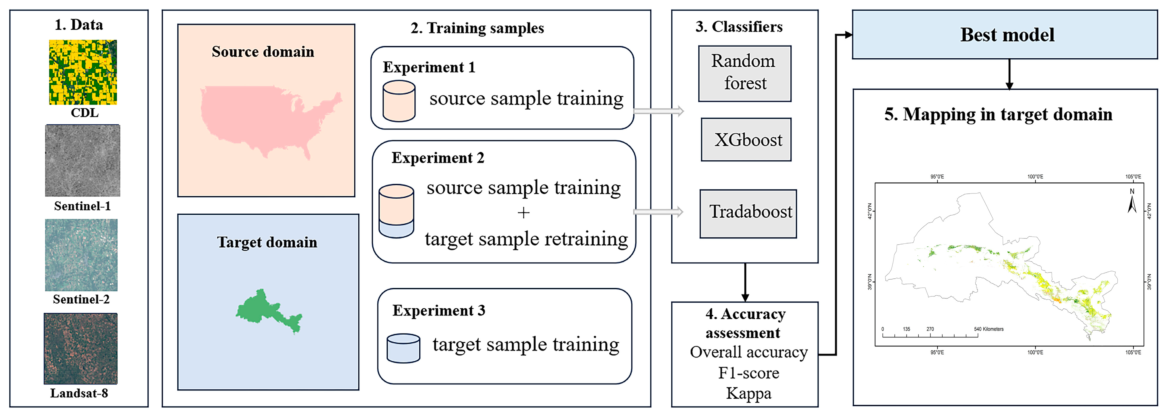

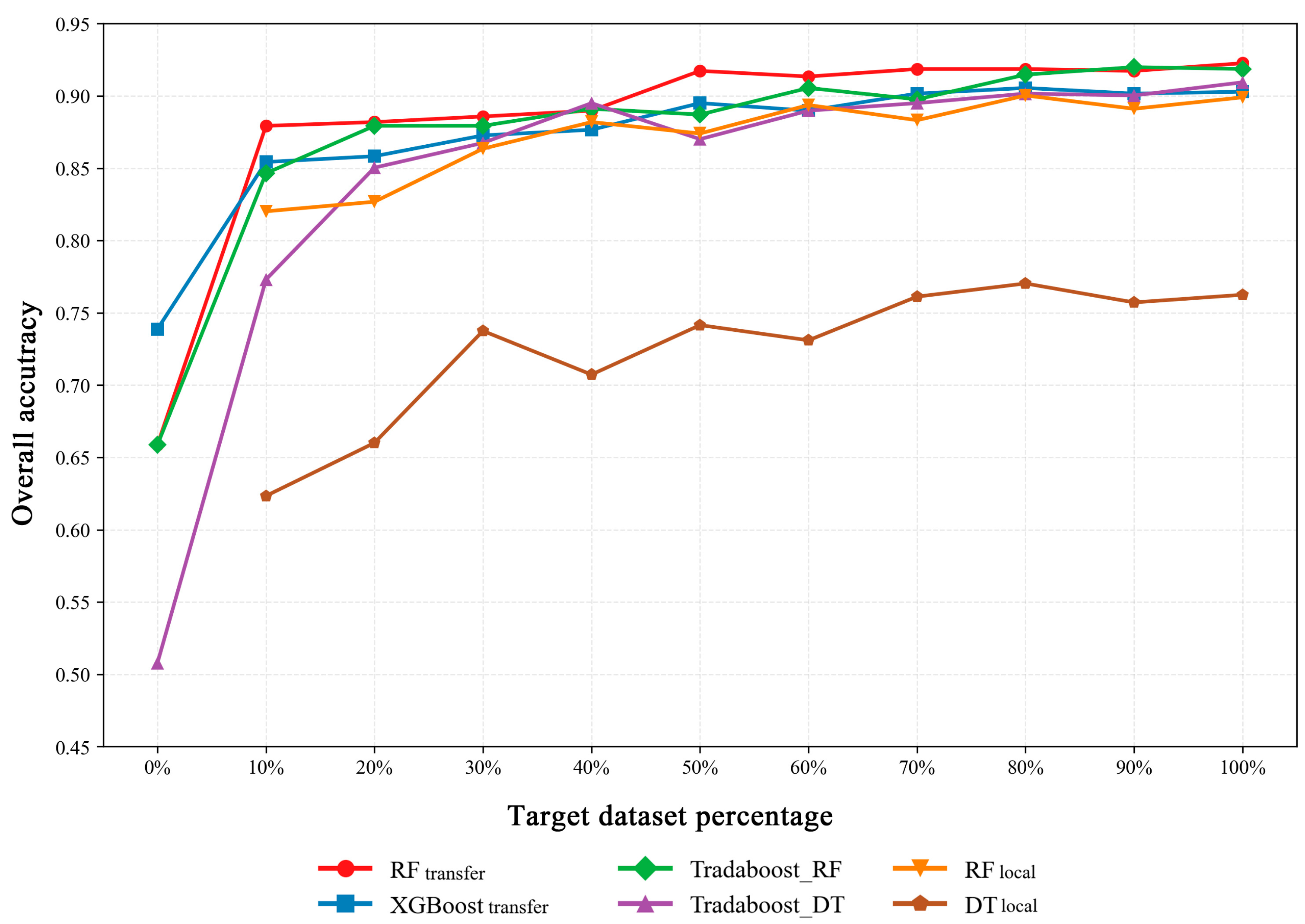
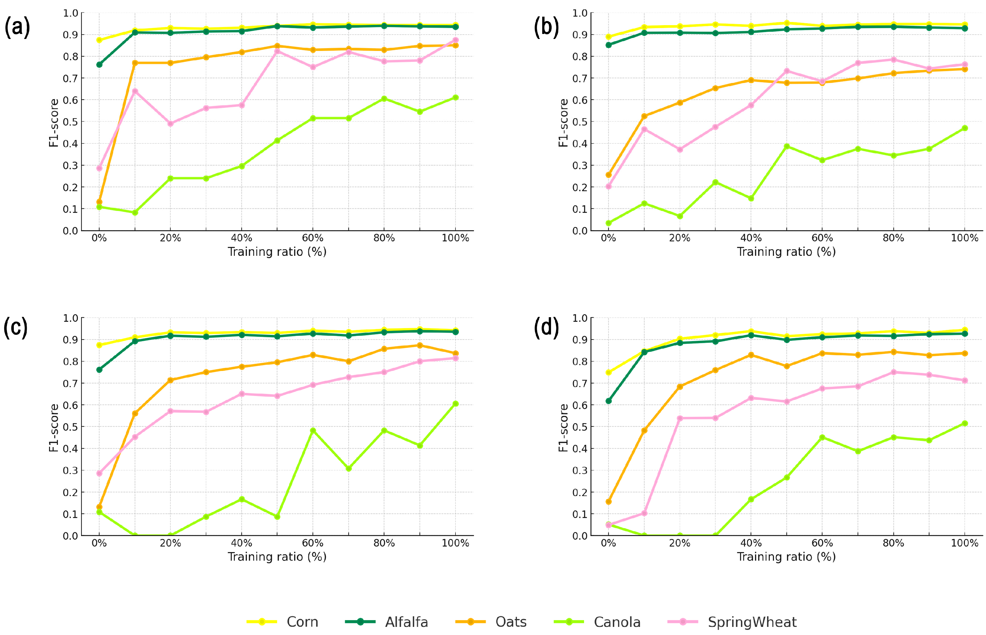


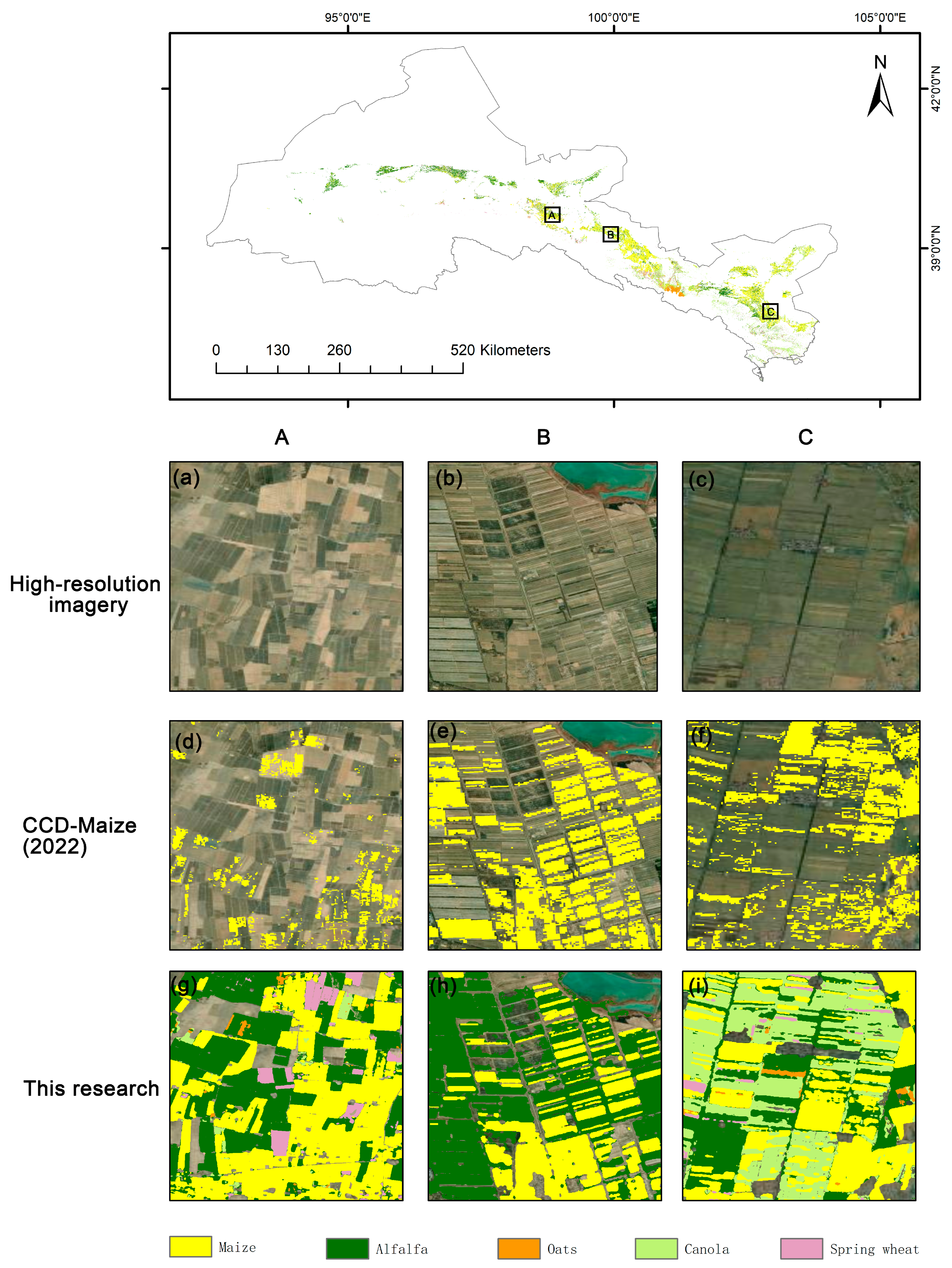
Disclaimer/Publisher’s Note: The statements, opinions and data contained in all publications are solely those of the individual author(s) and contributor(s) and not of MDPI and/or the editor(s). MDPI and/or the editor(s) disclaim responsibility for any injury to people or property resulting from any ideas, methods, instructions or products referred to in the content. |
© 2025 by the authors. Licensee MDPI, Basel, Switzerland. This article is an open access article distributed under the terms and conditions of the Creative Commons Attribution (CC BY) license (https://creativecommons.org/licenses/by/4.0/).