Article

Airborne Streak Tube Imaging LiDAR-Based Effective Reconstruction of Urban Water Areas

1
National Key Laboratory of Science and Technology on Tunable Laser, Harbin Institute of Technology, Harbin 150001, China
2
Space Representative Office, Changchun 130000, China
*
Author to whom correspondence should be addressed.
Remote Sens. 2026, 18(16), 2689; https://doi.org/10.3390/rs18162689
Submission received: 23 May 2026 / Revised: 5 August 2026 / Accepted: 6 August 2026 / Published: 10 August 2026

Highlights

What are the main findings?
  • This method effectively extracts the features of weak underwater echo signals from streak tube lidar and precisely enhances their intensity through the design of MADRA and STDFBlock, restoring richer water area information.
  • The model achieves competitive performance while maintaining low parameter counts and demonstrates good robustness toward degraded weak echo streak images.
What are the implications of the main findings?
  • This framework provides an effective enhancement scheme for weak echo signals in LiDAR 3D imaging, delivering valuable data for reconstructing richer regional information and identifying targets with low reflectivity.
  • This work offers a practical, efficient solution for precise enhancement of images containing fine structural details, applicable to identifying and extracting features of streak-like objects such as highways in remote sensing and blood vessels in medical imaging.

Abstract

When LiDAR detects underwater targets, the water severely attenuates the laser beams, making it impossible to extract valid echo information during 3D reconstruction of urban water bodies. This study proposes a Multi-Scale Spectral Adaptive Loss Generative Adversarial Network Based on Morphology-Spatiotemporal Decoupled Attention (MSAGAN) that effectively enhances far-field underwater echo signals for LiDAR. Its core components consist of three parts: Morphology-Aware Dynamic Receptive Field Attention (MADRA), Spatial-Temporal Decoupled Frequency-Enhanced Global Feature Fusion Block (STDFBlock), and Adaptive Dynamic Adjustment Loss Function Based on Frequency-Domain Decomposition and Gradient Response (FGADLoss). The model precisely identifies the narrow and curved local structures of the echo signals during the feature extraction process, improving the precise detection of subtle structural changes in the echo signals and enabling the extraction of valid echo signal features from a background of numerous invalid echo signals. The model reduces image fragmentation and center-of-mass drift during echo signal augmentation, improving the accuracy of water body environments’ 3D reconstruction. Through this model, the average point cloud density per square meter for lakes and ponds increased by 2.12 and 3.54, respectively, enabling effective reconstruction of urban water bodies information and offering a high-quality data basis for underwater object recognition and bathymetric surveying. Furthermore, this method effectively addresses the challenge of simultaneously obtaining degraded and ideal streak images that match the echo signals of underwater detection targets, and it also offers advantages in terms of training data requirements, making it particularly well-suited for real-world underwater detection scenarios where paired ideal-degraded data is scarce.

1. Introduction

Lidar possesses picosecond-level temporal resolution capability and active range discrimination characteristics, enabling high-precision terrain mapping [1,2,3] and target detection [4,5,6,7]. Among these, airborne streak tube imaging LiDAR (ASTIL) provides high mobility, rich echo semantic information, and full-waveform echo data sampling. Additionally, the ASTIL blue-green laser matches the water attenuation window, allowing for good underwater penetration and making it appropriate for underwater target recognition and terrain identification [8,9,10,11]. While Fang [12] showed that streak tube LiDAR can effectively recover complex details of targets detected in indoor still water using denoising and deblurring techniques under low signal-to-noise ratio conditions, the water significantly attenuates the laser signal when ASTIL’s laser travels across a complicated water environment. As a result, the received echo signal streak image is severely degraded, making it impossible to extract meaningful information. Consequently, subsequent steps such as streak image processing and target detection and identification become difficult to implement. Therefore, proposing a method for precisely enhancing the streak patterns in underwater echo signals is of great significance.
Currently, underwater image enhancement algorithms are primarily divided into three categories: non-physical model-based enhancement methods, physical model-based enhancement methods, and deep learning-based enhancement methods.
Non-physical model-based enhancement methods [13,14,15] do not take into account the underwater imaging process. For example, methods based on histogram equalization directly improve images through techniques such as histogram stretching without considering the physical processes underlying underwater image degradation. Enhanced images obtained through non-physical model-based methods often exhibit artifacts or excessive enhancement, and may even damage the image structure, resulting in unsatisfactory results.
Building a physical model of the underwater image deterioration process [16,17,18] is the main idea underpinning physics-based enhancement methods, such as those based on prior physical knowledge. Establishing a physical degradation model, estimating the unknown parameters within the model, and substituting the parameters into the model to solve the inverse problem are the primary steps of physics-based enhancement methods. The establishment of physical models for underwater imaging relies on prior knowledge and statistical characteristics; moreover, parameter estimation struggles to comprehensively account for different aquatic environments, resulting in a lack of strong generalizability.
Deep learning has demonstrated exceptional performance in image processing applications such as style transfer, super-resolution, image enhancement, and image denoising in recent years. Image processing has made extensive use of convolutional neural networks (CNNs). Dong [19] proposed using deep CNNs to learn end-to-end mappings between low-resolution and high-resolution images. This network, termed SRCNN, demonstrated high-quality performance in classical super-resolution computer vision problems. Li [20] proposed an underwater image enhancement convolutional neural network called UWCNN based on underwater scene priors. Using underwater scene prior knowledge, this model synthesizes deteriorated underwater datasets across various water types and degradation levels before performing enhancement specific to each underwater environment. Applications of generative adversarial networks (GANs) in image processing have advanced significantly. Pix2Pix, a network model based on conditional generative adversarial networks, was proposed by Isola [21] and shown to be effective for image-to-image translation applications, especially those with highly structured image outputs. CycleGAN, a GAN-based system that learns to translate between domains without paired input examples, was presented by Zhu [22] and showed impressive results in a variety of circumstances. Islam [23] presented FUnIEGAN, a conditional GAN-based real-time underwater image enhancement technique that learns to enhance underwater images through paired and unpaired training. The enhanced images improved the performance of standard models in tasks such as underwater target detection. Fabbri [24] proposed UGAN, a technique that uses generative adversarial networks to improve the quality of underwater visual scenes. This model first generates paired images for training, then reconstructs underwater datasets using a U-Net architecture to obtain enhanced underwater color images; Wang [25] proposed an unsupervised generative adversarial network based on an improved underwater imaging model, called UWGAN, to generate realistic underwater images from aerial and depth images. This model first creates paired images for training before reconstructing underwater datasets using a U-Net architecture to obtain enhanced underwater color images.
Although fully supervised learning produces amazing picture improvement outcomes, these techniques strongly rely on the quality of the training set and require tight alignment between low- and high-quality photos for training. Because these files are frequently unavailable, this is especially difficult for underwater images. The original cycle consistency loss function fails to achieve high-precision reproduction of the original image’s structure and content in the generated images since it simply imposes color constraints on the input and reconstructed image. The neural network augmentation models mentioned above frequently use synthetic datasets for training because underwater datasets are hard to come by. However, synthetic datasets cannot fully simulate the degradation processes of underwater images. Most improvements focus on RGB color correction and contrast enhancement for images obtained through passive underwater imaging, while few algorithms address the precise enhancement of original details and structures in images derived from active underwater imaging. Furthermore, using fixed-size convolution kernels for feature extraction can easily lead to the loss of image information.
In order to tackle these issues and challenges, we suggest a Multi-Scale Spectral Adaptive Loss Generative Adversarial Network Based on Morphology-Spatiotemporal Decoupled Attention (MSAGAN). The following are the primary innovations:
(1) MSAGAN can effectively address the challenges posed by ASTIL underwater weak echo signals—where active imaging is required, paired training datasets are difficult to obtain, and streak structures within the same region exhibit high similarity, making it challenging to extract feature differences. It achieves more accurate, pixel-level three-dimensional spatial coordinates for underwater targets.
(2) Morphology-Aware Dynamic Receptive Field Attention (MADRA) and Spatial-Temporal Decoupled Frequency-Enhanced Global Feature Fusion Block (STDFBlock) were combined to create a multi-attention mechanism. MADRA enhances the model’s ability to detect valid echo signals across different scales and structures and to extract intricate streak structural features. It can accurately distinguish the narrow and curved local structures of echo signals, enabling precise separation of streak structural information against a background of numerous invalid echo signals. This prevents the loss of valid echo signals and enhances the continuity and integrity of streak structures during downsampling. The STDFBlock interacts with channel information from multiple perspectives to capture global features. It achieves an explicit separation of low-frequency structures and high-frequency details in the frequency domain to generate global channel weights, which enhances the model’s ability to perceive important channel features. Additionally, it introduces a resolution-enhancing attention mechanism, which enhances the model’s precise identification of subtle changes in streak microstructure.
(3) Adaptive Dynamic Adjustment Loss Function Based on Frequency-Domain Decomposition and Gradient Response (FGADLoss) strengthens the constraint that the fine structure and content of streak remain unchanged during the image enhancement process. It enhances the generator’s ability to accurately distinguish between clusters of sparse echo signal pixels and background pixels, which reduces the occurrence of streak breaks during enhancement; it also effectively suppresses shifts in the center of mass of streak caused by rigid translation and non-rigid morphological distortions.

2. Materials and Methods

2.1. Operating Mechanism of Airborne Streak Tube Imaging LiDAR

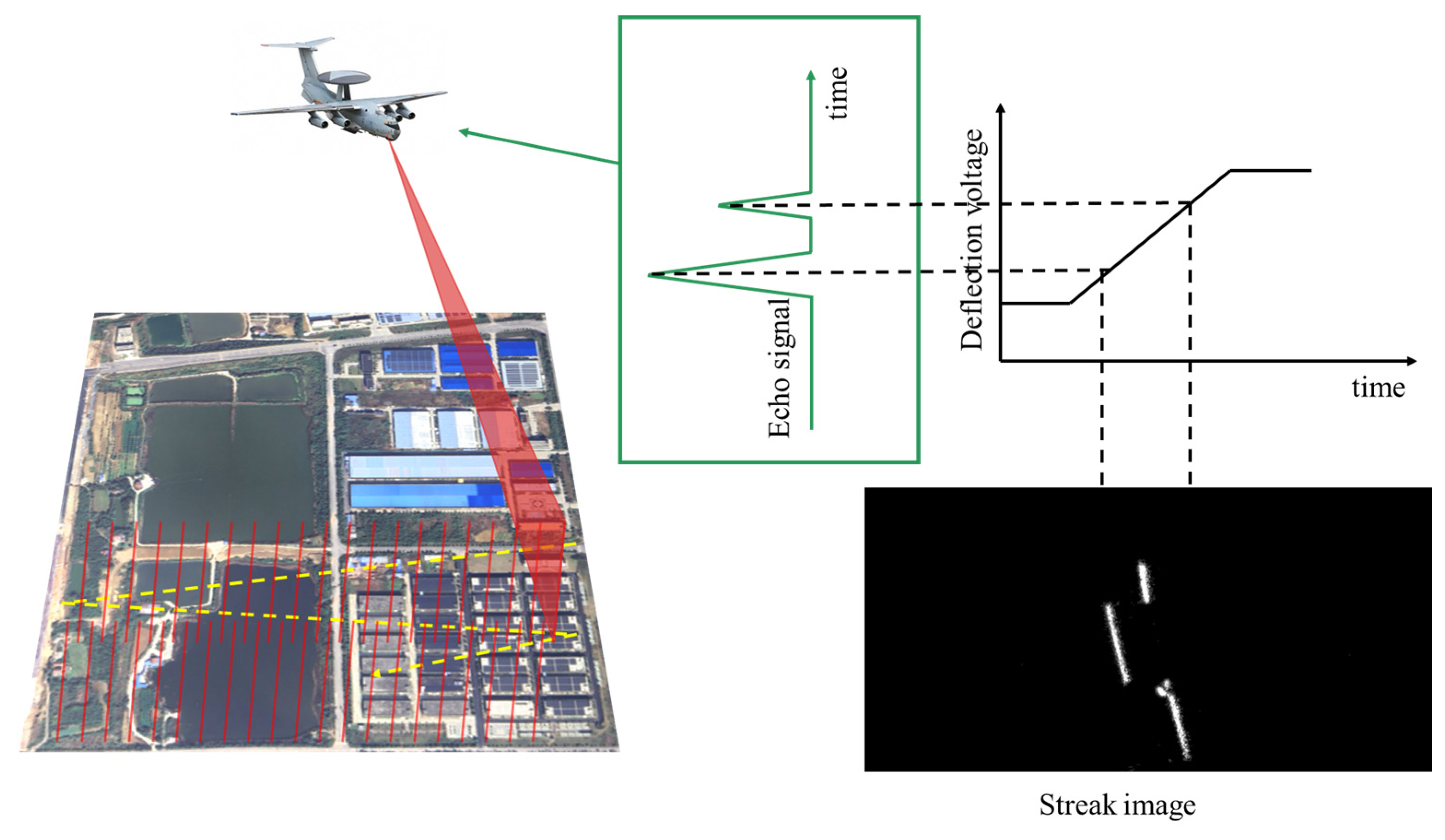
ASTIL uses a “swing” scanning mode, in which the optical axis traces a zigzag path on the ground along the aircraft’s flight path via the scanning system, as shown by the yellow dashed line in Figure 1. The scanning path in this operating mode follows a zigzag pattern along the aircraft’s flight path, enabling a wider scanning area.
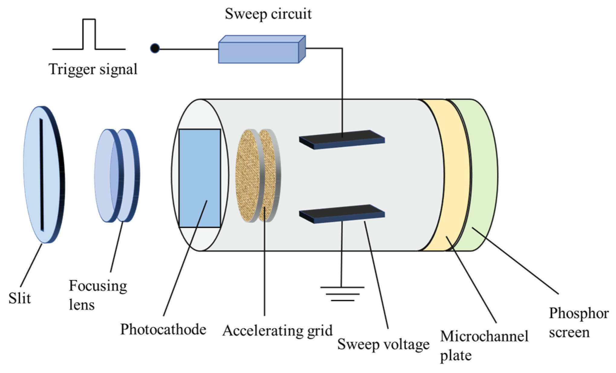
Figure 2 shows the structure of the streak tube imaging unit. ASTIL’s signal acquisition system consists of a streak tube imaging unit and a charge-coupled device (CCD) connected downstream. Since the periodic scanning voltage from the electron deflection system is applied perpendicular to the optical axis, the laser pulses returning at different times under the influence of the deflection voltage are mapped as streak information at different positions in the CCD image.

2.2. Modules and Framework of the Model

2.2.1. Morphology-Aware Dynamic Receptive Field Attention

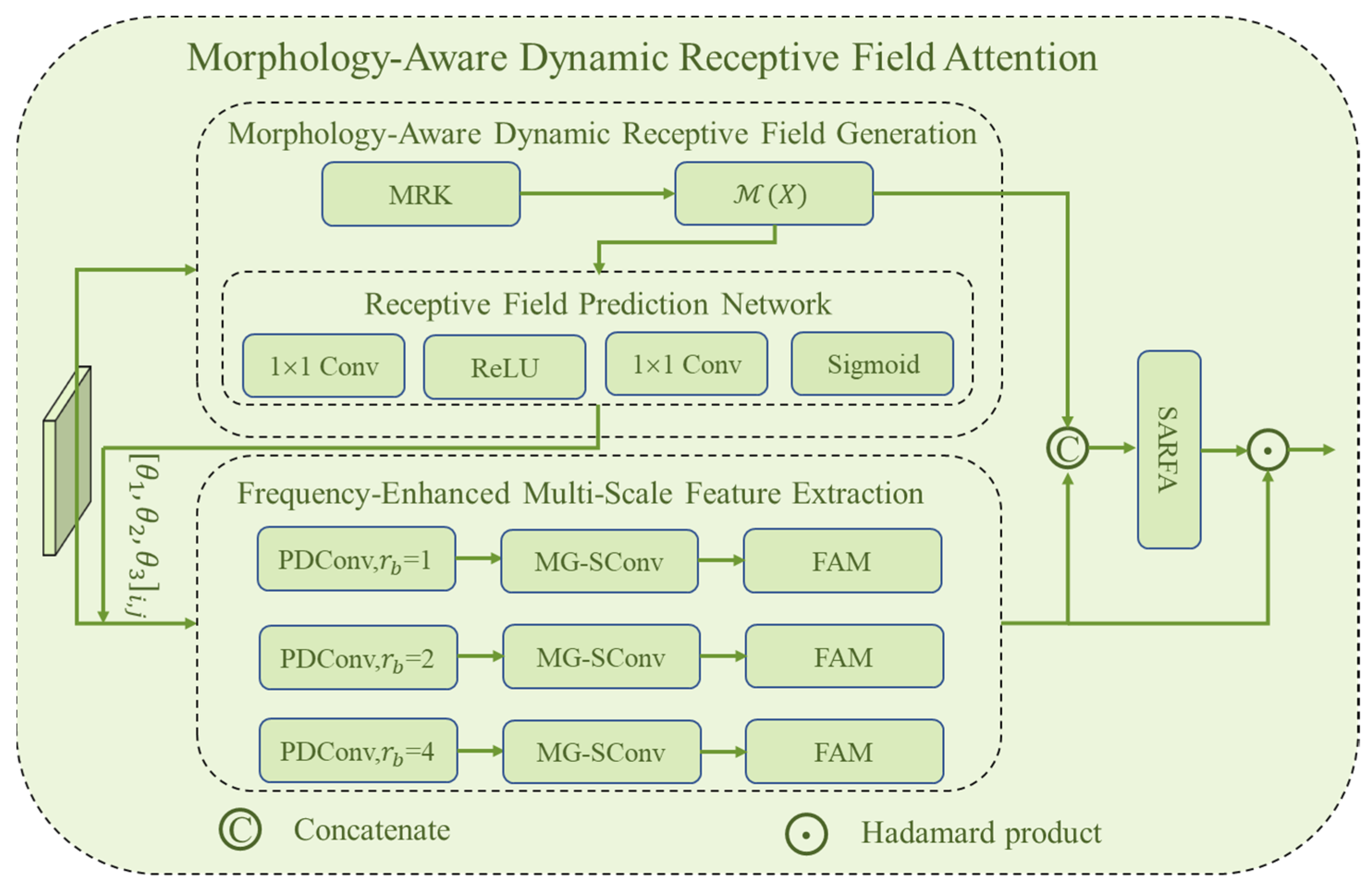
The structural information contained in the underwater echo signal streak image (UESSI) reflects topographical variations within the detection region and changes in the elevation of detection targets. Maintaining consistent structural information in streak images throughout the enhancement process is critical for achieving high-precision detection with LiDAR. However, only a tiny percentage of the streak image is made up of streak information; the majority is made up of black regions that are devoid of echo signals. Neural networks may find it challenging to extract streak features when streak information is not spatially dominating because the backdrop may dampen signals from objects of interest. There is limited chance of recovery during training if the target signal is lost as a result of downsampling. Additionally, the neural network’s capability to extract features from underwater echo signals is diminished since basic neural networks’ fixed-size convolution kernels are unable to extract features from intricate structural transformations, potentially resulting in the loss of image information. Within the same UESSI, regions with dense strong signals require small receptive fields to accurately preserve local details, while regions with weak signals require large receptive fields to infer signal continuity using contextual information. To address these challenges, we propose Morphology-Aware Dynamic Receptive Field Attention (MADRA). The overall architecture of MADRA consists of three submodules connected in series: Morphology-Aware Dynamic Receptive Field Generation Module (MDRF), Frequency-Enhanced Multi-Scale Feature Extraction (FEMFE), and Spatially Adaptive Receptive Field Aggregation (SARFA). The network architecture diagram is shown in Figure 3.
The core task of MDRF is to dynamically generate optimal receptive field configuration parameters for each spatial location based on the morphological structure of the input feature map. We introduce a learnable Morphological Response Kernel (MRK) and Receptive Field Prediction Network (RFPN) to achieve content-adaptive generation of receptive field parameters. Unlike traditional convolutions that use fixed weights to extract spatial features, MRK consists of a set of differentiable morphological operators. Specifically, for an input feature X , MRK computes a local morphological descriptor at each spatial location:
M ( X ) i , j =   [ G r a d x ( X ) i , j , G r a d y ( X ) i , j ,   C u r v ( X ) i , j ,   E n t r o p y ( X ) i , j   ]
where G r a d x and G r a d y represent the gradient magnitudes in the horizontal and vertical directions, respectively, characterizing the local orientation and edge intensity of the streak signals; C u r v is a local curvature estimate, reflecting the degree of curvature of the streak; E n t r o p y is a measure of local information entropy, used to distinguish signal-dense regions from sparse background regions.
This morphological descriptor provides structure-aware prior information for the subsequent dynamic prediction of receptive fields, enabling the model to comprehend the type of image structure at each location and thereby generate matching receptive field parameters.
After obtaining the morphological descriptor M ( X ) , the RFPN is responsible for predicting the optimal receptive field configuration parameters for each spatial location. The RFPN consists of two layers of 1 × 1 convolutional kernels and nonlinear activation functions, mapping the morphological descriptor to a three-dimensional receptive field configuration vector:
Θ i , j =   σ ( W 2   · R e L U ( W 1   ·   M ( X ) i , j ) )
where Θ i , j = [ θ 1 ,   θ 2 ,   θ 3 ] i , j is the three-dimensional receptive field configuration vector at position ( i , j ) , corresponding to dilation coefficient θ 1 [ 0 ,   1 ] , used to dynamically adjust the equivalent dilation rate of subsequent convolutional kernels, thereby achieving spatial adaptive fine-tuning of the receptive field scale; deformation amplitude coefficient θ 2 [ 0 ,   1 ] , which controls the scale of the deformation offset in snake convolution; frequency modulation coefficient θ 3 [ 0 ,   1 ] , used to adjust the gain factors of each frequency band in the frequency enhancement module; σ is the Sigmoid activation function, ensuring that the predicted receptive field configuration parameters Θ are normalized to serve as smooth, continuous modulation factors; ReLU is a rectification function that introduces nonlinear expressive capability as an activation function; W 1 and W 2 are learnable weight matrices in the fully connected layer. W 1 performs linear transformation and nonlinear mapping on the input morphological descriptor M ( X ) to extract deep features for predicting the receptive field, while W 2 maps the extracted features to the final three-dimensional receptive field configuration parameters Θ .
In the UESSI streak feature extraction task, the MDRF ensures that θ 1 tends toward smaller values in signal-dense regions to enable fine-grained local perception, while in signal-sparse regions, θ 1 tends toward larger values to facilitate context-based inference. Additionally, in regions with high curvature, θ 2 is set to a larger value to enhance adaptability to serpentine bending. This dynamic generation mechanism enables each neuron to obtain the optimal receptive field configuration based on the morphological characteristics of its location.
The FEMFE module receives the receptive field configuration vector Θ generated by MDRF and performs multiscale feature extraction across three parallel feature extraction branches. FEMFE integrates Parametric Dilated Convolution (PDConv), Morphology-Guided Snake Convolution (MG-SConv), and Frequency Adaptive Modulation (FAM) into each branch.
The base dilation rate for each branch of PDConv is set to 1, 2, and 4, respectively, to cover a multiscale range from local details to global semantics. PDConv receives the dilation rate coefficient θ 1 output by MDRF and performs continuous fine-tuning at the spatial position level near the base dilation rate via a learnable mapping function, enabling the receptive field scale to be finely calibrated according to local morphological features. The dilation rate of PDConv is dynamically determined by θ 1 ; if the branch index is k { 1 ,   2 ,   3 } , then the dilation rate of the kth branch is:
r k ( i , j ) =   r k b a s e +   r ·   tanh α · θ 1 ( i , j )
where r k b a s e represents the base dilation rate, which is initially set to 1, 2, and 4 in this paper; r is the maximum adjustable range; α is the scaling factor, which allows the dilation rate to be continuously fine-tuned around the base value according to the streak structure.
The dilation rate and the dilation rate coefficient θ 1 output by the MDRF are continuously adjusted around the base value. This design enables the receptive field size at each spatial location to be precisely calibrated according to its morphological features—the receptive field is automatically reduced in signal-dense regions to preserve local details, and automatically expanded in signal-sparse regions to infer structural continuity using contextual information. This approach ensures both the breadth of multiscale coverage and fine-grained calibration at each spatial location.
MG-SConv concatenates the morphological descriptor M ( X ) generated by MDRF with the input feature map along the channel dimension, then inputs them together into the offset generation convolution. The offset is globally scaled via the deformation amplitude coefficient θ 2 :
( i , j ) =   γ ·   θ 2 ( i , j )   · ( W o f f s e t [ X , M ( X ) i , j ] )
where [ · , · ] denotes the concatenation operation for channel dimensions; γ is the global scaling factor; W o f f s e t represents the convolution kernel weight of the convolution layer that generates deformable convolution offsets.
The introduction of M ( X ) guarantees that the deformation direction is simultaneously constrained by morphological information, such as curvature and edge orientation, rather than being purely determined by local gradients. This maximizes the preservation of signal structure continuity and integrity during downsampling by enabling the snake convolution’s kernel shape to more closely match the true geometric trajectories of the echo signal streak in UESSI and the narrow and curved local structures within the echo signals.
FAM first converts the feature maps of each branch into the frequency domain using the Fast Fourier Transform, obtaining the amplitude spectrum A k and the phase spectrum P k . The amplitude spectrum is further decomposed into three subbands: low-frequency, mid-frequency, and high-frequency A k = { A k l o w , A k m i d , A k h i g h } . Then FAM uses the frequency modulation coefficient θ 3 output by the MDRF to generate the adaptive gain for each subband:
A k e n h =   A k l o w · ( 1   + λ l o w θ 3 ) + A k m i d · ( 1   + λ m i d ) + A k h i g h · ( 1   + λ h i g h θ 3 )
where λ l o w ,     λ m i d ,     a n d   λ h i g h are learnable frequency band weighting coefficients.
The gain for the mid-frequency subband remains fixed, whereas the low- and high-frequency subbands receive a gain factor relating to θ 3 . The signal is restored to the spatial domain using the Inverse Fast Fourier Transform after the enhanced amplitude spectrum is combined with the original phase spectrum.
In UESSI-enhanced tasks, the edges and texture information of the streak signal are primarily distributed in the high-frequency subbands, while background noise typically occupies the low-frequency components. FAM is designed as an asymmetric frequency modulation mechanism aimed at maintaining the stability of mid-frequency information and ensuring that the continuity of streak edges is not disrupted by dynamic modulation. Additionally, it provides flexibility for both high-frequency and low-frequency components to be dynamically adjusted. It effectively improves the model’s capacity to capture details in weak echo signals while suppressing the propagation of background interference in the feature space by selectively enhancing high-frequency responses and moderately suppressing low-frequency components.
The SARFA module reconstructs the weight allocation mechanism in the form of spatial attention, enabling each pixel location to independently select the optimal receptive field size based on its morphological features. SARFA first concatenates the feature maps from the three branches with the morphological description operator M ( X ) from MDRF along the channel dimension. It then generates branch selection probabilities for each spatial position across the three branch feature maps output by FEMFE using a 1 × 1 convolutional layer and a Softmax activation function. The final output feature map is obtained by combining the three resulting weight scores with the feature maps using a spatially weighted Hadamard product and element-wise summation. The incorporation of morphological description operators enables the distribution of attention weights to be sensitive to image structure: at signal edges, higher weights are assigned to small-receptive-field branches to preserve details, while within the signal, higher weights are assigned to large-receptive-field branches to infer structural integrity using contextual information. This spatially adaptive aggregation strategy enables MADRA to dynamically configure optimal receptive field combinations for regions of different characteristics in UESSIs—dense signal regions, sparse signal regions, and signal-free background regions. This effectively prevents information loss in complex heterogeneous image content during downsampling caused by a single receptive field, providing high-quality multiscale feature representations for subsequent upsampling reconstruction of the generator.

2.2.2. Spatial-Temporal Decoupled Frequency-Enhanced Global Feature Fusion Block

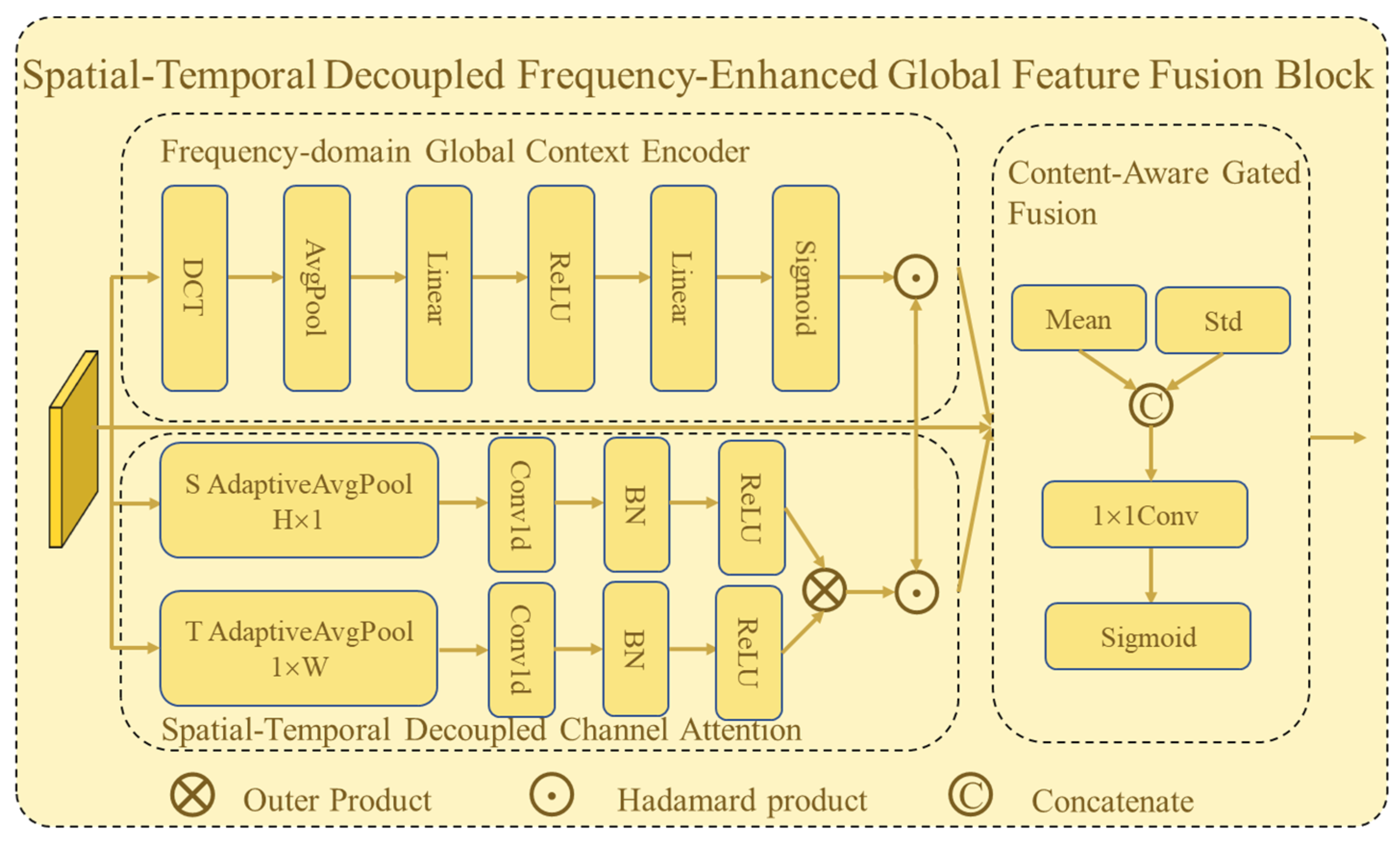
The deflection electric field direction in ASTIL’s streak tube possesses time resolution capability, while the perpendicular direction to the deflection electric field provides spatial resolution capability [26]. These two axes are respectively termed the time axis and the spatial axis. Each row parallel to the time axis can be represented as a time resolution channel, and each column parallel to the spatial axis can be represented as a spatial resolution channel. This is manifested in the streak image as the position coordinates of the echo signal pixels. In the streak image generated by the echo signal, the horizontal coordinate of each pixel reflects the target’s distance information, while the vertical coordinate reflects the target’s spatial position information. ASTIL determines the spot position by locating the center of mass within the echo signal streak image [27,28], thereby calculating the laser’s time-of-flight and spatial information to compute the precise location of the detected target. During image augmentation, unsupervised neural networks may cause shifts in the position of the center of mass, which could lead to larger errors in both the temporal and spatial resolution of ASTIL as well as a decrease in target detection accuracy. Additionally, the generated streak images from echo signals show great similarity when terrain variations within the same detection area are minor, making it simple for the neural network to ignore these minor variations throughout the learning process. We suggest Spatial-Temporal Decoupled Frequency-Enhanced Global Feature Fusion Block (STDFBlock) as a solution to these problems. STDFBlock consists of three components: Frequency-domain Global Context Encoder (FGCE), Spatial-Temporal Decoupled Channel Attention (STDC), and Content-Aware Gated Fusion (CAGF); the network architecture diagram is shown in Figure 4. STDFBlock significantly enhances the neural network’s ability to capture global contextual information and multi-view channel relationships. Its parallel-structure design and the introduction of a channel attention mechanism facilitate information exchange and feature fusion across different branches, enabling the effective integration of transformed multi-scale features. The channel attention mechanism enables the model to adaptively learn the importance weights of each channel, enhancing the model’s perception of subtle details by increasing the weights of key channels.
While high-frequency components encode the edges and local texture details of the echo signals, low-frequency components carry the majority of the global structure of streak images. Conventional spatial-domain global pooling compresses high-frequency and low-frequency information indiscriminately, causing the latter to contaminate the former. FGCE transforms the input feature map into the frequency domain via a two-dimensional discrete cosine transform (DCT). UESSI’s primary structure and content information are highly concentrated in the low-frequency coefficients, while high-frequency textures are distributed across coefficients far from the origin. The DCT possesses excellent energy compression properties. Based on this property, FGCE retains only the low-frequency subbands of the DCT coefficients for global context encoding, enhancing the module’s global perception capabilities. It explicitly separates low-frequency structures from high-frequency information, fully preserving high-frequency details for independent processing by subsequent local attention branches, thereby avoiding the irreversible damage to fine-scale structural information caused by global pooling. The global frequency-domain description vector z is obtained by applying global average pooling to the truncated low-frequency coefficients obtained by DCT using a preset low-frequency truncation threshold. A global frequency-domain weight vector is then generated by passing this vector z through a channel weight generator made up of two fully connected layers. These weights reflect the importance of each channel at the global structural level and can adaptively enhance the ability to extract streak structural features.
STDC completely decouples the temporal and spatial attention calculations for streak images into two independent parallel subbranches: the spatial attention branch and the temporal attention branch. The spatial attention branch compresses the information of each channel in the horizontal dimension into a one-dimensional description in the vertical direction for the input feature map X by performing average pooling along the temporal axis to extract channel attention responses regarding the target spatial location in the vertical direction. One-dimensional convolution is then used to aggregate local neighborhood information along the vertical direction, and normalization and a Sigmoid activation function are used to create a spatial attention weight vector. This weight vector reflects the relative importance of each channel at different spatial locations along the vertical direction and can adaptively enhance the channel response to changes in the corresponding target’s spatial position. The temporal attention branch compresses the input feature map along the spatial axis to extract channel attention responses regarding target distance information in the horizontal direction, similarly generating a temporal attention weight vector. This vector encodes the sensitivity of each channel to changes in target distance information in the horizontal direction. Finally, the spatial and temporal attention weights are fused into a complete spatio-temporal attention map through an outer product operation.
In UESSIs, regions with sparse weak echo signals need stronger feature enhancement to compensate for information loss during downsampling, while features in dense strong echo signal regions are easily learned and excessive enhancement may introduce artifacts. CAGF provides a differentiated fusion strategy for different regions. CAGF first calculates the local mean and local standard deviation at each spatial position along the channel dimension for an input feature map X . The local mean reflects the overall signal intensity at that spatial location, while the local standard deviation quantifies the texture complexity and the degree of abrupt variation in features within that region. A two-channel statistical feature map is created by concatenating these two components along the channel dimension. The statistical features are then mapped to a spatially adaptive gating factor γ using a 1 × 1 convolution and a Sigmoid activation function, generating an independent adaptive gating factor γ ( i , j ) for each spatial location that is sensitive to the content features of each local region. The final output feature map uses gated weighted fusion to combine the original features with the enhanced features, which have been modulated by both spatiotemporal attention and global weights in the frequency domain. This mechanism enhances regions with strong signals more significantly to highlight key features, while preserving more original information in regions with weak signals and background areas to maintain stability, thereby achieving pixel-by-pixel differentiated control over the enhancement intensity across different image regions.


2.2.3. Network Framework of MSAGAN

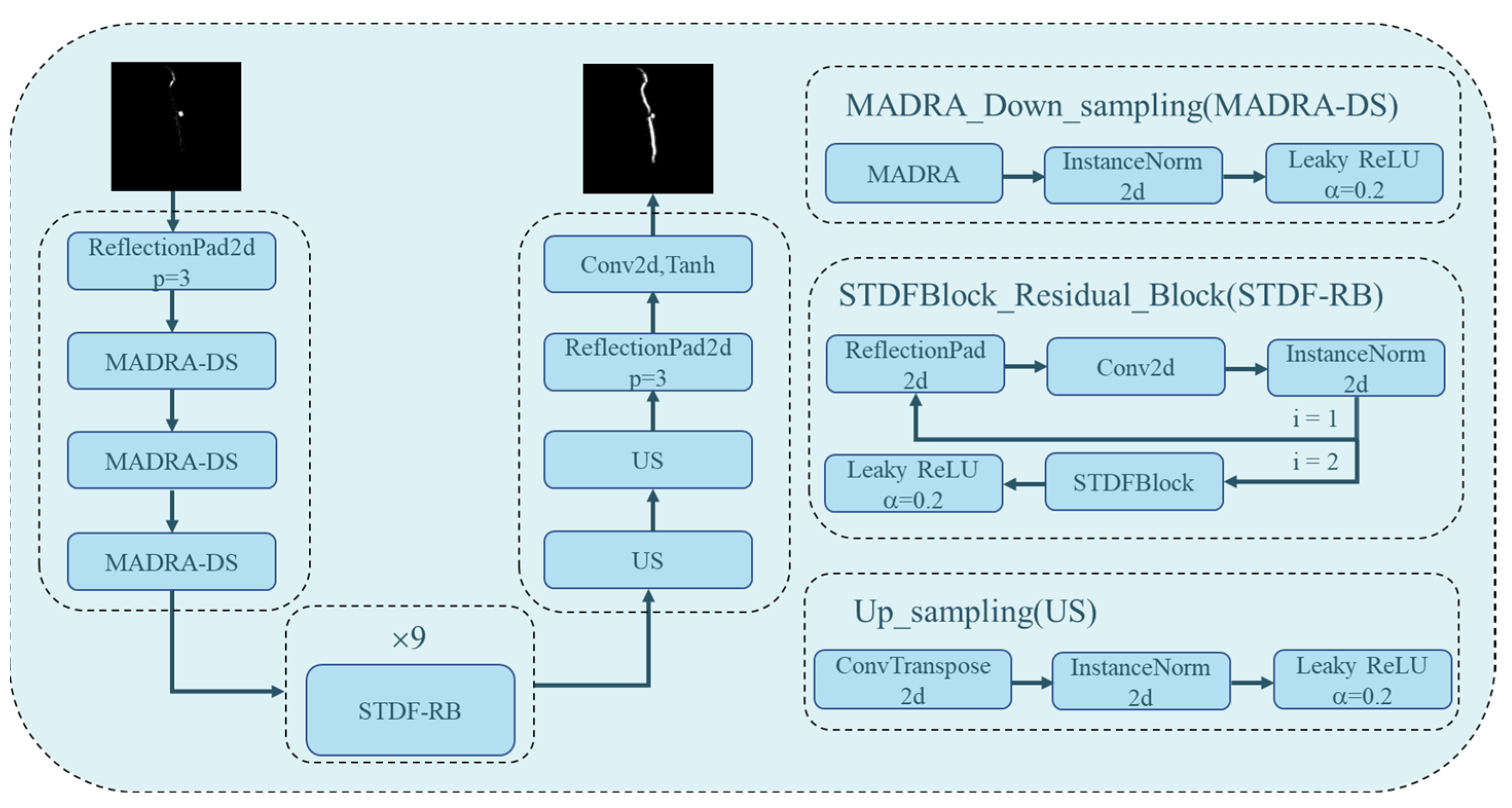
In the MSAGAN network, the CycleGAN [22] framework serves as the backbone for UESSI enhancement, consisting of two generators and two discriminators. Figure 5 shows the MSAGAN network’s generator. In order to prevent information loss during convolution operations, UESSI first uses the ReflectionPad2d function to fill the boundaries of the streak image using mirror mode. The padded image then passes through the MADRA encoder, which consists of three serial subsampling layers incorporating the MADRA mechanism, increasing the channel count from 1 to 256. Subsequently, the feature maps are passed through nine repeated residual blocks that incorporate the STDFBlock module—collectively referred to as the STDFBlock transformation module—followed by two serial upsampling layers that restore the initial resolution. Lastly, precisely enhanced UESSI is produced by the output layer, which consists of ReflectionPad2d, a convolutional layer, and a Tanh activation function.
The MSAGAN network’s two discriminators are the discriminator Dx for the weak echo signal domain X and the discriminator Dy for the strong echo signal domain Y. The discriminators use the five feature extraction activation blocks of the PatchGAN design. Each block employs a “convolution-BN-activation” structure. The first four layers employ a 4 × 4 convolutional kernel with a stride of 2, utilizing the LeakyReLU activation function with a slope of 0.2. The final layer employs a 3 × 3 convolutional kernel with a stride of 1, employing the Sigmoid activation function. The input image is divided into several overlapping local regions by PatchGAN, which then independently outputs true-or-false assessments for each region. This improves the model’s capacity to extract more information about important regions and learn local image information.

2.3. Loss Function

2.3.1. Adaptive Dynamic Adjustment Loss Function Based on Frequency-Domain Decomposition and Gradient Response

During training, unsupervised generative adversarial networks (GANs) are typically weakly constrained. The majority of current bidirectional GANs concentrate mostly on learning interdomain cycle consistency and global domain appearance, frequently producing less-than-ideal outcomes when it comes to capturing high-frequency information and local details. Additionally, the effective streak information in UESSI constitutes only a small portion of the streak image, with a limited number of pixel groups. During feature extraction, background information can interfere with these tiny structures, making it impossible to fully capture the entire content of the echo signal. This often causes the generator to produce broken and centroid-shifted streaks when generating enhanced streak images. We suggest Adaptive Dynamic Adjustment Loss Function Based on Frequency-Domain Decomposition and Gradient Response (FGADLoss) as a solution to the above issues. FGADLoss achieves a more refined and self-consistent multidimensional joint supervision of the streak enhancement process by introducing Spectrum Adaptive Gradient Loss ( L S p e c G r a d ), Wavelet domain high frequency loss ( L W a v H F ), and Local Structure Contrastive Loss ( L C o n t r a ) and supplementing with training state-based Gradient-Loss Dual Adaptive Mechanism (GL-DAM).
L S p e c G r a d enforces multi-scale structural and content alignment in the gradient domain to preserve edge sharpness and structural information. Constraints are constructed at the intersection of the gradient and frequency domains, where a set of fixed bandpass filters decomposes the gradient difference between the generated and target images into three frequency bands—low-frequency contours, mid-frequency edges, and high-frequency textures—and applies respective constraints to each:
L S p e c G r a d =   E x , y [ s = 1 S ω s ( t ) · H s ( G ( x ) y ) 1 ]
where G ( x ) is the enhanced image generated by the generator; y is the real target image; is the spatial gradient operator, used to extract structural edge information from the image; H s is the s-th scale of learnable spectral modulation filter banks, used to decompose the gradient map into different frequency subbands; in this paper, S = 3, and H 1 employs a large-scale Gaussian blur kernel to preserve the broad-scale contours and brightness trends in UESSI; H 2 employs a Gaussian difference filter to preserve mid-frequency structures such as the streak structure and sharp edges in UESSI; H 3 is a high-pass filter that directly subtracts the low-frequency components from the original gradient map to obtain a residual map containing the finest edges and textures; ω s ( t ) represents the dynamic attention weights at the s-th scale at training time t .
L W a v H F performs a first-order discrete wavelet transform on both the generated image and the target image, directly targeting high-frequency components. This forces the model to learn the spectral differences between real echo signals and background noise, effectively suppressing the masking effect of background noise on weak signals. By matching local high-frequency features, it achieves position-aware detection, providing positional constraints for pixels and effectively suppressing rigid translations and non-rigid morphological distortions.
L W a v H F = o { L H , H L , H H } W 1 , o ( G ( x ) ) W 1 , o ( y ) 1
where W 1 , o denotes the high-frequency subband coefficients of the first-order discrete wavelet transform in the horizontal, vertical, and diagonal detail directions, which are used to extract features of the echo signal at the finest scale.
L C o n t r a imposes discriminative constraints on echo signal regions and non-echo signal regions in the feature space. This loss function forces the generated features to be close to the source image features in the latent space for regions belonging to valid echo signals; for background or noise regions, it forces their feature representations to maintain sufficient cosine distance from signal regions and background regions of different samples. This ensures that the local feature representations of the generated image resemble their corresponding positions in the original image while maintaining discriminative separation from features of unrelated regions, enabling the generator to precisely distinguish between signal pixel clusters and background pixel clusters and avoid generating discontinuous streaks. This loss function extracts local feature vectors from the feature maps of the generator’s intermediate layers and calculates the normalized temperature cross-entropy between these vectors and the positive sample features at the corresponding source image locations, as well as other negative sample features within the same batch:
L C o n t r a =   log e x p ( s i m ( f v , f v + ) / τ ) e x p ( s i m ( f v , f v + ) / τ ) + j = 1 K e x p ( s i m ( f v , f v , j ) / τ )
where f v is the local patch feature vector extracted from the feature map of the generator’s intermediate layer at position v ; f v + is the corresponding feature vector from the source image at the same position, serving as positive sample pairs; f v denotes the patch feature vectors from other positions randomly sampled within the same batch, serving as negative sample pairs; K represents the number of negative sample pairs; s i m ( · , · ) denotes cosine similarity; τ is the temperature parameter.
GL-DAM normalizes the ratio of gradient norms across different loss components to achieve adaptive balance in gradient magnitude, preventing any single gradient from becoming too dominant and dominating the overall optimization direction. By using a Sigmoid activation function to control the intervention intensity of each component at different training stages, it enables an adaptive transition from pixel-level alignment to structural refinement and ultimately to semantic alignment; Through feedback on the rate of loss decline, the weight of a loss component automatically decreases as the decline of a loss component approaches saturation, directing optimization resources to other dimensions where there is still room for improvement. Weight coefficients λ k ( t ) ( k { S G , W , C } for each loss component are uniformly generated by GL-DAM. This mechanism decomposes the weight into the product of the gradient pathway Φ g r a d and the loss pathway Ψ l o s s :
λ k ( t ) =   α k · Φ g r a d ( t ) ·   β k · Ψ l o s s ( t )
where α k is the base scaling coefficient of the training path, which controls the extent to which gradient difficulty perception contributes to the final weights, α k = [ 1 ,   1 , 1 ] to ensure that the gradient path remains unbiased; β k is the base scaling coefficient of the loss path, which controls the extent to which loss convergence perception contributes to the final weights, β k = [ 1.2 ,   0.8 ,   0.8 ] to incorporate prior knowledge into the loss function; the gradient path Φ g r a d measures the current optimization difficulty of the task via the gradient norm ratio: Φ g r a d ( t ) =   θ L k 2 1 3 j { S G , W , C } θ L j 2 , where θ represents the generator parameters and calculates the gradient of the loss function with respect to the model parameters; θ L k denotes the gradient vector of the kth loss with respect to the generator parameters θ . It calculates the gradient norm ratio of the current component to the generator parameters. A larger gradient norm indicates that the current parameters have not yet been sufficiently optimized for the task, and thus their weights should be dynamically increased. The loss pathway Ψ l o s s measures the convergence rate of the task as a linear ratio of the current loss to its initial value: Ψ l o s s ( t ) = L k ( t ) L k ( 0 ) + ϵ , where t is the current training iteration step; ϵ is a minimal smoothing constant to prevent division by zero; L k ( t ) is the current value of the kth loss at time t; L k ( 0 ) is the initial value of the kth loss at the start of training. The greater the decrease in the loss value relative to the initial value, the closer the model is to convergence. In this case, the weight should be reduced to prevent overfitting and suppress the optimization of other objectives, shifting the optimization focus to loss terms that have not yet fully converged.
The general expression for FGADLoss is as follows:
L F G A D ( t ) =   λ S G ( t ) L S p e c G r a d + λ W ( t ) L W a v H F + λ C ( t ) L C o n t r a
where L S p e c G r a d represents the Spectrum Adaptive Gradient Loss; L W a v H F represents the Wavelet domain high frequency loss; L C o n t r a represents the Local Structure Contrastive Loss; λ k ( t ) ( k { S G , W , C } ) represents the dynamic weight coefficients, which are adaptively generated by the GL-DAM mechanism based on real-time gradients and the convergence status of the loss.

2.3.2. Loss Function of MSAGAN

The adversarial loss function uses a least squares generative adversarial network (LSGAN) [29] to create an adversarial game between the generator and the discriminator. For the process of mapping the weak echo signal domain X to the strong echo signal domain Y, the adversarial interaction is established between the generator G and the discriminator D Y :
L GAN ( G ,   D Y ,   X ,   Y )   =   E y ~ p data ( y ) [ ( D Y ( y ) 1 ) 2 ]   +   E x ~ p data ( x ) [ D Y ( G ( x ) ) 2 ]
Discriminator D Y aims to maximize the objective function in order to accurately distinguish real strong echo signals y from generated samples G(x). Conversely, generator G seeks to minimize the generation term in this function—that is, by optimizing its parameters so that the generated images approximate the statistical distribution of the real domain Y, thereby deceiving the discriminator into outputting a high-confidence score.
Following the principle of dual generative adversarial networks, a similar adversarial loss is introduced for the generator F and the discriminator D X during the mapping from the strong echo signal domain Y to the weak echo signal domain X: L GAN ( F ,   D X ,   Y ,   X ) .
FGADLoss guarantees that an image is restored as closely as possible to the original image when it is translated from the source domain to the target domain and then back to the source domain by introducing a cyclic consistency loss function:
L cyc ( G ,   F )   =   E x ~ p data ( x ) [ L FGAD ( F ( G ( x ) ) ,   x , t ) ]   +   E y ~ p data ( y ) [ L FGAD ( G ( F ( y ) ) ,   y , t ) ]
FGADLoss employs an identity loss function to force the generator to maintain an identity mapping when processing images from the target domain, thereby avoiding unnecessary modifications to images that already belong to the target domain:
L identity ( G ,   F )   =   E x ~ p data ( x ) [ L FGAD ( F ( x ) ,   x , t ) ]   +   E y ~ p data ( y ) [ L FGAD ( G ( y ) ,   y ,   t ) ]
where t is the current iteration number; X and Y denote the weak and strong echo signal domains, respectively; x and y denote images in the weak echo signal domain and the strong echo signal domain, respectively; D Y is the discriminator that determines whether the converted image G ( x ) is authentic in comparison to the Y domain image; D X is the discriminator that determines whether the converted image F ( y ) is authentic in comparison to the X domain image; E y ~ p data ( y ) and E x ~ p data ( x ) denote the mathematical expectations of images sampled from the training data distribution for the strong echo signal domain Y and the weak echo signal domain X , respectively.
The loss function for MSAGAN is shown in Equation (14):
L   =   L GAN ( G ,   D Y ,   X ,   Y )   +   L GAN ( F ,   D X ,   X ,   Y )   +   λ cyc L cyc ( G ,   F )   +   λ id L identity ( G ,   F )
where L GAN denotes the generative adversarial loss function; L cyc denotes the cyclic consistency loss function; L identity denotes the identity loss function; λ cyc is the weight coefficient for the cyclic consistency loss function; λ id is the weight coefficient for the identity loss function.

2.4. ASTIL Point Cloud Inversion System

2.4.1. Echo Signal Centroid Extraction

The streak images generated by ASTIL echo signals correspond one-to-one with the laser’s footprint at the target. To perform point cloud inversion, it is necessary to obtain distance and position information representing the target pixels. In actual detection, the laser generates multiple echo signals when it passes through building edges or vegetation, which appear as multiple spots in a single row of the streak image. Consequently, it is necessary to extract several centers of mass. As shown in Algorithm 1, the method for extracting multiple centers of mass is as follows: The entire algorithm consists of two passes that transform the streak image into a center-of-mass matrix. First, a left-to-right single-sided pass identifies valid spot regions in each row where all consecutive grayscale values exceed the threshold T g and the number of consecutive points is at least T n . Through statistical analysis of the data from the test area, the value of T g was set to 20, and that of T n was set to 5 pixels. The geometric center of each region is taken as the center of mass for that spot, and the maximum value k of the number of spots counted in each row is used as the number of columns in the output center-of-mass matrix. Then, the algorithm performs another row-by-row traversal, sequentially filling the initial matrix with the centroids extracted from each row. Once the traversal is complete, the center-of-mass matrix is output.
Algorithm 1. Center of Mass Matrix Extraction
Input: Echo Signal Streak Image I R 512 × 1024 ,   T g , T n
Output: Center-of-Mass Matrix of Echo Signals C R 512 × k
1.function extract_row_centroids(line, Tg, Tn):
2.centroids = []
3.m = len( I )
4.n = len(line)
5.idx = 0
6.while idx < n:
7.        if line[idx] > Tg:
8.                start = idx
9.                while idx < n and line[idx] > Tg:
10.                        idx = idx + 1
11.                end = idx − 1
12.                length = end − start + 1
13.                if length >= Tn:
14.                        center = (start + end)/2
15.                        centroids.append(center)
16.        else:
17.                  idx = idx + 1
18.return centroids
19.function main( I , Tg, Tn):
20.        k = 0
21.        for i = 0 to m − 1:
22.                row_centroids = extract_row_centroids( I [i], Tg, Tn)
23.                k = max(k, len(row_centroids))
24.         C = matrix(m, k)
25.        for i = 0 to m − 1:
26.                row_centroids = extract_row_centroids( I [i], Tg, Tn)
27.                for k = 0 to len(row_centroids) − 1:
28.                         C [i][k] = row_centroids[k]
29.        return  C

2.4.2. Data Fusion

During point cloud inversion, it is necessary to know the spatial position and orientation of the sensor at the exact moment each laser pulse is emitted; this position and orientation information is provided jointly by the Global Positioning System (GPS) and the Inertial Measurement Unit (IMU). Due to differences in physical principles and design constraints, the sampling rates of different sensors often vary. In this experiment, the GPS and IMU have a sampling rate of 200 Hz, while the STIL has a sampling rate of 2000 Hz. If the nearest POS data were directly paired with each laser pulse, motion-induced positioning errors would cause systematic distortions in the point cloud, which would be particularly severe when the platform changes speed or turns. To address this issue, an interpolation strategy is employed during data fusion: using the ASTIL’s 2000 Hz timestamps as a reference, the 200 Hz POS time series is interpolated to generate position and attitude parameters that are strictly synchronized with each laser pulse.

2.4.3. Coordinate Transformation

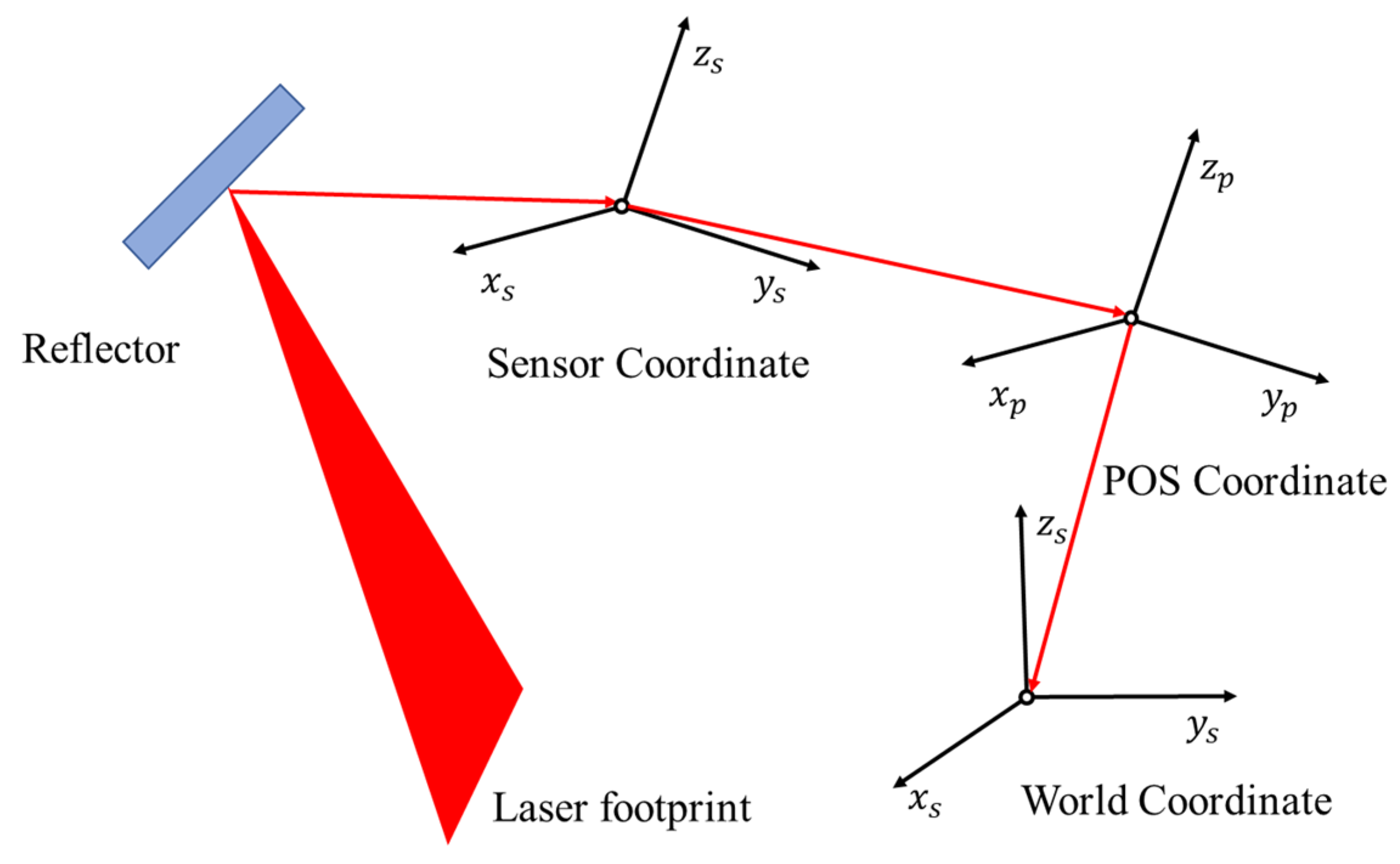
As shown in Figure 6, the distance and incident vector from the streak imaging system are back-calculated to the laser footprint via the scanning system and ultimately represented in the world coordinate system using POS data; this process involves transformations between multiple coordinate systems. First, the center-of-mass position of each spot in the streak image is mapped to the distance ρ and scan angle θ in the sensor coordinate system using pre-calibrated system geometric parameters. The sensor coordinate system is then converted to the POS coordinate system, with the IMU’s reference center serving as the origin, using a rigid transformation. Next, the longitude, latitude, and altitude of the POS data are converted into three length measurements in the XYZ coordinate system. Combined with the three angular measurements from the POS, the coordinates of the target point are transformed into an XYZ coordinate system centered at the Earth’s center, and finally, the XYZ coordinate system is converted to the WGS-84 coordinate system.

3. Results

3.1. Dataset and Evaluation Preparation

3.1.1. Dataset for Underwater Echo Signal Enhancement

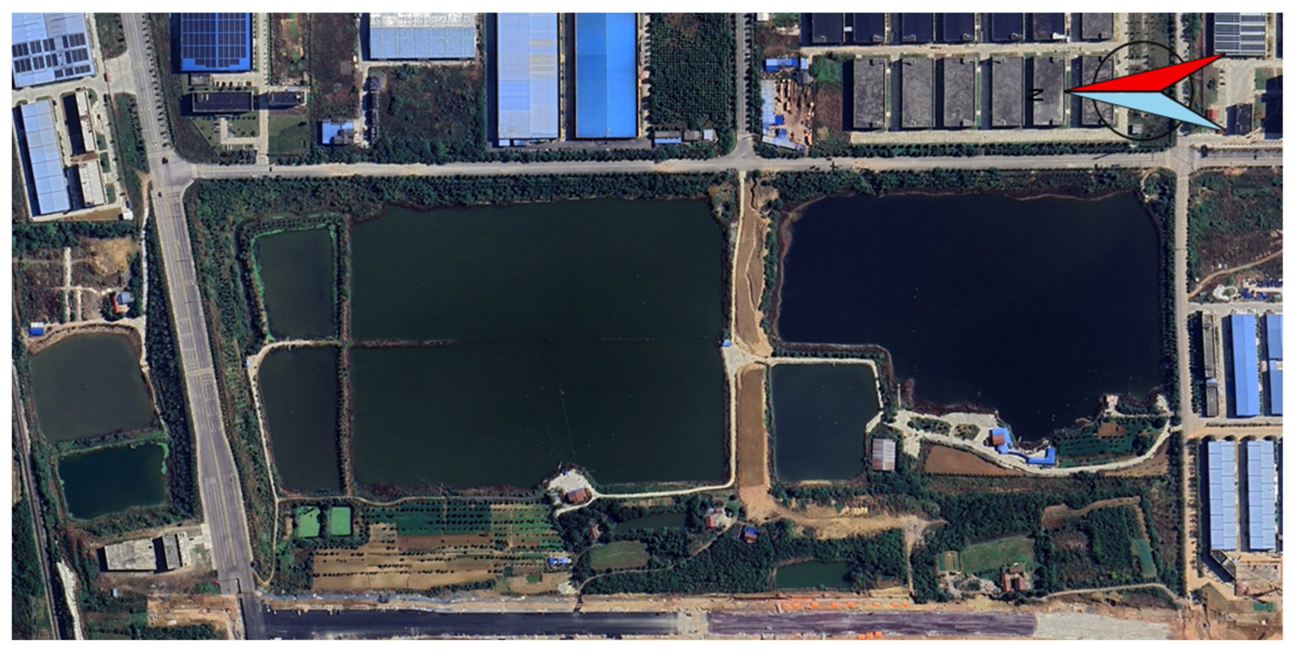
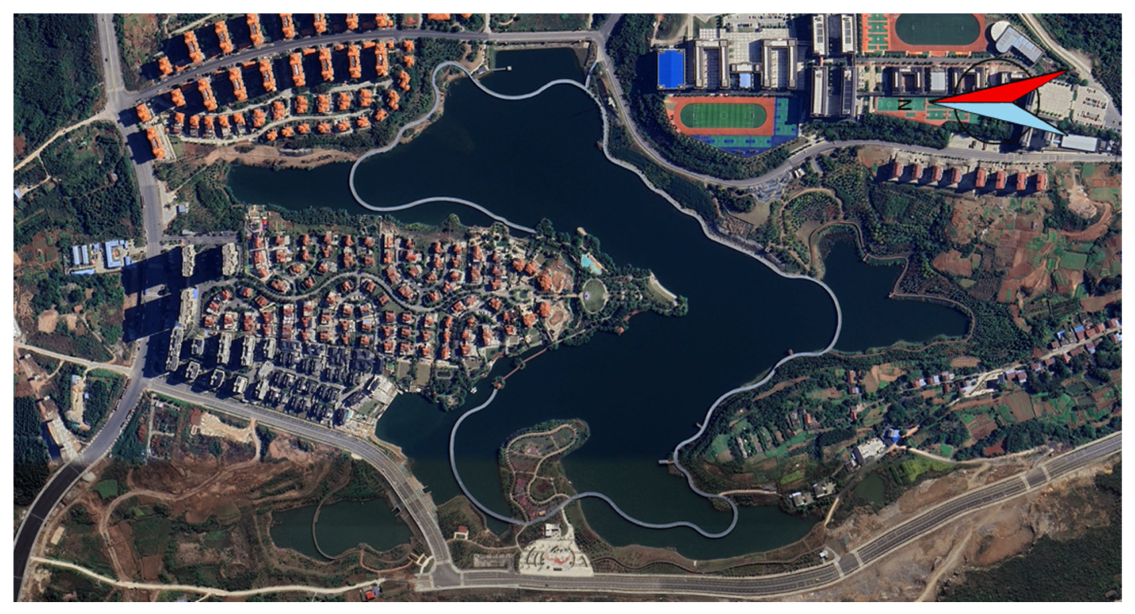
As seen in Figure 7 and Figure 8, the dataset used in this paper was collected during field experiments in 2023. The detection area is located in Jingmen City, Hubei Province, China, at an altitude of approximately 100 m. The flight platform operated at an altitude of approximately 3000 m during data collection. The ASTIL laser [30] operated at a repetition rate of 2000 Hz, with a wavelength of 532 nm, a pulse width of 6.4 ns, and a range resolution of 15 cm, generating streak images with a resolution of 512 × 1024 pixels from the returned echo signals. The large size of the raw echo signal streak image introduces a substantial number of trainable parameters during training, prolonging the model’s convergence time. The remaining portions of the streak image constitute useless regions devoid of echo signal information beyond the pixel points generated by effective underwater echo signals. UESSI can be preprocessed before training to speed up the training of the model because effective echo information is only distributed in the central portion of the streak image. The effective echo signal center of mass is determined as the image center by calculating the x-coordinate of the UESSI center of mass. The image is then expanded 256 pixels to the left and right, yielding a 512 × 512 effective streak image as the input image. The start and end positions of the cropped image are stored in a dictionary format for restoration after image enhancement. The echo signals from ground targets exhibit the least attenuation because laser propagation in air encounters minimal obstructing material. These serve as ideal echo signal streak images for MSAGAN training. There are 3982 underwater echo signal streak images and 10,266 ground echo signal streak images (GESSI) in the dataset. Details of the various datasets are shown in Table 1.
Python 3.10 and PyTorch 1.12 were used in the experimental environment configuration for this work. The hardware platform included Windows 10, 256 GB of RAM, and an Nvidia GeForce Quadro GP100. The initial learning rates for both the generator and discriminator are set to 0.0002, with a batch size of 1 per GPU. The maximum number of training epochs is set to 500. Additionally, an early stopping criterion is employed: training is halted prematurely if the loss fails to decrease for ten consecutive epochs, indicating that the model has converged.

3.1.2. Experimental Evaluation Indicators

We used four key evaluation metrics to assess the performance of the suggested model: Structural Similarity Index (SSIM), Peak Signal-to-Noise Ratio (PSNR), Learner-Perceived Image Block Similarity [31] (LPIPS) and Centroid Drift Measure (CMD). To quantitatively evaluate the enhancement performance of echo signals in the enhanced images, ground strong-echo streak images were adopted as references. Ground echo streak images not participating in training were chosen based on the similarity of their streak skeletons to those of the underwater streak images, which correspond to various underwater terrain types, such as flat and sloping regions. These selected ground strong echo images were then degraded to simulate underwater echo signals. Finally, the degraded ground echo signals, after being enhanced by each model, were quantitatively evaluated.
SSIM measures the structural similarity between two images based on three aspects: luminance, contrast, and texture.
S S I M ( x , y ) = ( 2 μ x μ y + c 1 ) ( 2 σ x y + c 2 ) ( μ x 2 + μ y 2 + c 1 ) ( σ x 2 + σ y 2 + c 2 )
where μ x and μ y denote the mean values of image x and image y , respectively; σ x and σ y denote the standard deviations of image x and image y , respectively; σ x y denotes the covariance between image x and image y ; c 1 and c 2 are regularization constants introduced to prevent computational instability caused by excessively small denominators.
PSNR measures image quality by comparing the mean squared error between the reference image and the enhanced image:
P S N R = 10 · l o g 10 ( I m a x 2 M S E )
where I m a x stands for the maximum possible value of image pixels; M S E is the mean squared error, which represents pixel differences between images and is computed as follows: M S E =   1 M N i = 1 M j = 1 N [ a ( i , j ) a ^ ( i , j ) ] 2 , where M and N represent the total number of pixels in the M × N image; a ( i , j ) and a ^ ( i , j ) represent the corresponding grayscale values in the reference image and enhanced picture, respectively.
LPIPS captures higher-level features of images through learning and is more sensitive to distortions in details and textures:
L P I P S ( x , x 0 ) =   l 1 H l W l h , w ω l     ( y ^ h w l y ^ 0 h w l ) 2 2
where l denotes the index of the feature layer in the neural network; H l and W l represent the height and width of the l th-layer feature map; h and w represent spatial position indices within the feature map; y ^ h w l and y ^ 0 h w l denote the feature vectors extracted from the enhanced image x and reference image x 0 at the l th layer and spatial position (h, w), respectively; ω l is a learnable weight vector reflecting the varying importance of feature channels in perceiving differences.
CMD evaluates the enhancement accuracy by calculating the mean of the ratio between the difference in each row’s centroid coordinates prior to and following augmentation and the horizontal resolution of the image:
C M D = 1 N i = 1 N ( x x 0 ) H R
where N denotes the number of rows in the image; x and x 0 represent the centroid positions of pixels per row before and after enhancement, respectively; H R denotes the horizontal resolution of the image.

3.2. Experimental Results

3.2.1. Comparative Experiments of Different Underwater Image Enhancement Models

The experimental conclusions were analyzed from both theoretical metrics and qualitative comparisons, including comparisons with more classical underwater image enhancement models. All models were trained using the same dataset and computer environment configuration, with the exception of CycleGAN and Pix2Pix, to guarantee a fair evaluation of each method. CycleGAN was trained on a dataset with more streak images to illustrate MSAGAN’s advantage in training sample requirements. In total, 4754 underwater echo signal streak images—1.6 times the size of the MSAGAN dataset—were utilized to train the CycleGAN neural network; Pix2Pix uses ideal-degenerate image pairs, but the paired training dataset is synthetically generated and is of the same size as that used by other neural networks. All models use the same test set to objectively evaluate their generalization ability after training is complete. The results for theoretical evaluation metrics such as PSNR, SSIM, LPIPS, and CMD are presented in Table 2:
A higher PSNR value indicates lower image distortion. Table 2 shows that both MSAGAN and Pix2Pix achieve favorable results when enhancing UESSIs, demonstrating a significant reduction in the introduction of anomalous noise points and artifacts during neural network training. A higher SSIM value indicates greater structural similarity between images. Table 2 shows that both SRCNN and MSAGAN achieve favorable results when enhancing UESSIs, demonstrating that during neural network training, they effectively balanced the structural information of streak patterns while ensuring the enhancement of high-frequency components. A lower LPIPS value indicates greater similarity in high-level features such as image details and textures. Table 2 shows that both SRCNN and MSAGAN achieve favorable enhancement performance on UESSIs, indicating the effective extraction of UESSI’s high-frequency information, texture structure, and other features during neural network training. A smaller CMD value indicates less center of mass offset during image enhancement, resulting in more precise 3D information in point cloud images generated from target echo signals. Table 2 shows that both SRCNN and MSAGAN achieve good results in enhancing UESSIs, demonstrating pixel-level accuracy in streak images during neural network training. While both Pix2Pix and SRCNN have shown promise in enhancing image evaluation metrics, Pix2Pix requires rigorous paired datasets for training, and SRCNN has not performed optimally in effectively enhancing images and restoring richer information from original echo signals. In contrast, MSAGAN-generated enhanced images are specifically tailored to address the scarcity of paired training datasets for underwater applications, in addition to achieving favorable results in theoretical metrics and accurately restoring underwater echo signals.
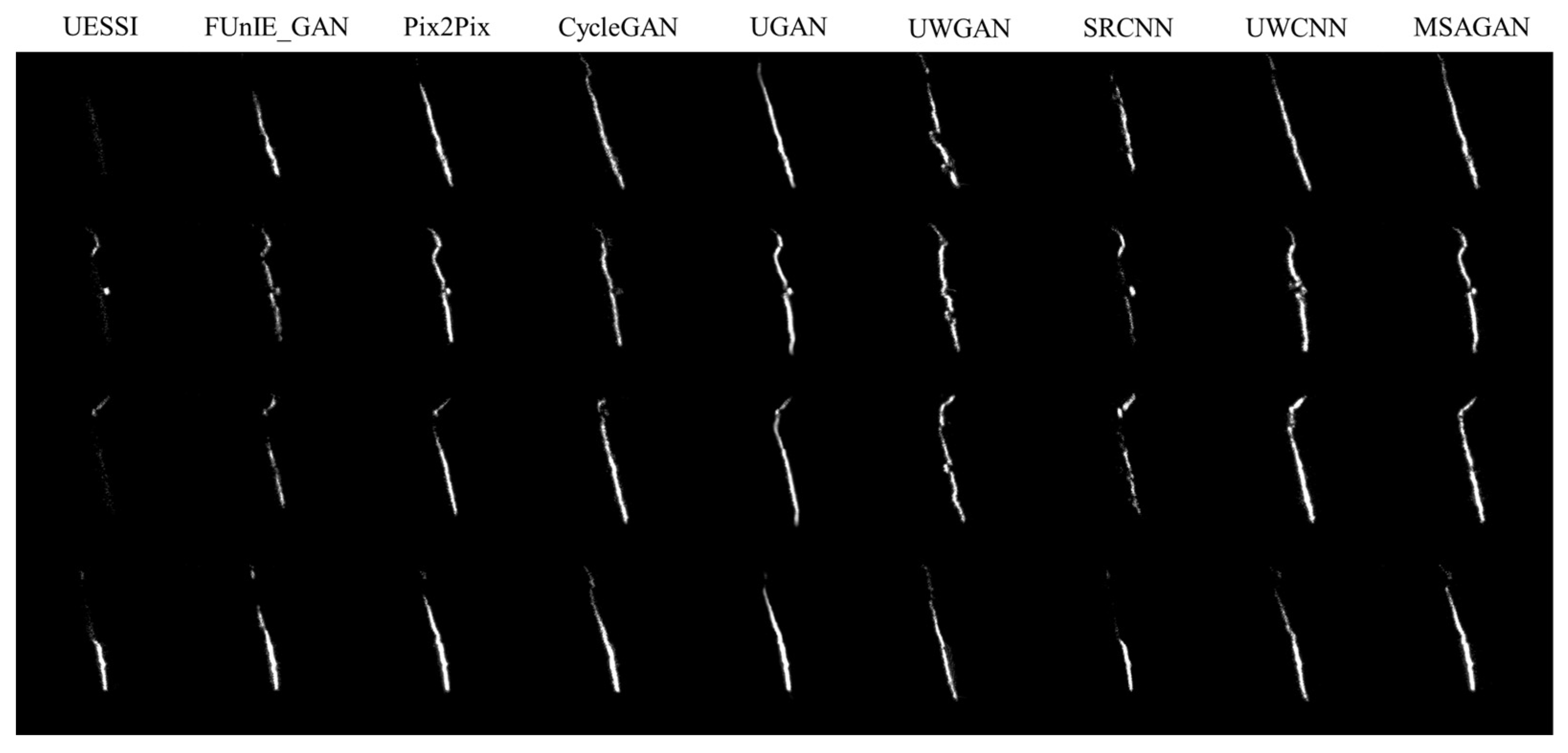
In UESSI’s raw echo streak images, the row coordinates directly reflect the target’s distance information, while the column coordinates correspond to the target’s spatial position in the scanning direction; the intensity information is closely related to the target’s reflection characteristics. Streak images provide a more concise and intuitive way to observe the structure and position of detected targets and can be used directly for target identification [32] and to assess the effectiveness of echo signal enhancement. The enhancing effects of four streak image types—all underwater echo signals, minimal surface echo signals, minor surface echo signals, and considerable surface echo signals—under various neural network training methods are depicted in Figure 9. For areas with stronger echo signals, FUnIEGAN shows better enhancement. However, it has trouble identifying original echo signal information in locations with weaker echo signals, which leads to poor retention of the original streak image structure and average enhancement performance. By improving the original streak images while retaining the majority of the original echo signal information, Pix2Pix produces good results. But in order to train Pix2Pix, paired training datasets are needed. Furthermore, it is difficult to capture both ideal and weakened streak images from the same place; CycleGAN shows poor learning performance, producing enhanced streak images with linear shape that were structurally similar and lost the original structure and substance of the echo signal. The structure and content information of the original echo signal was successfully retained using UGAN-enhanced streak images. Nevertheless, there is a visible haze in the enhanced images. This is due to the fact that the model uses CycleGAN to first degrade the streak images before obtaining paired datasets for training. Nevertheless, the underwater degradation environment cannot be completely simulated by the degradation network. During augmentation, UWGAN maintains the original echo signals’ structure and content information, but it introduces significant noise spots in the streak images’ high-frequency edge areas, making it difficult to detect target elevation information precisely. Although the high-resolution streak images enhanced by SRCNN achieved high scores in image evaluation metrics, it produces less than ideal enhancement effects for underwater echo signals since it is unable to efficiently extract the features of weak echo signals. Significant center-of-mass shifts are seen in UWCNN-enhanced streak images, which lowers the precision of target spatial location detection. In contrast, MSAGAN forces the enhanced image to restore the original streak echo signal pixel-level structure and content information. It improves the measurement of similarity between enhanced and original images at a high-level semantic level while reinforcing the learning of local texture structures and high-frequency edge information. Additionally, MSAGAN achieves more desirable results with fewer training sets, effectively addressing the challenges of small underwater image enhancement datasets and the scarcity of paired training data.
Figure 10 shows the point cloud images generated after the streak images of echo signals from ponds and lakes were enhanced using various neural network models. We can compare and analyze the accuracy of echo signal augmentation across different neural network models by examining Area A (the ring road around the lake), Area B (deep water), and Area C (shoreline trees) in the 3D point cloud photos of the lake. When UWCNN enhances underwater echo signals, the center of mass of the streak image shifts significantly, causing the information of the ring road in Area A to blend with that of the water, making it difficult to distinguish; when UGAN enhances underwater echo signals, the enhanced streak image exhibits a distinct misty effect, resulting in the ring road in Area A appearing rather blurry; The point cloud streaks generated in Area B of the enhanced echo signal streak images show signal-free regions along the edges due to FUnIEGAN’s enhancement characteristics, where strong underwater echo signals are significantly enhanced while weak signals show only moderate improvement; Although SRCNN improves the resolution of UESSI and achieves excellent results across all objective evaluation metrics, it does not fully recover all information from the underwater echo signal streak image, and the generated Area B still contains a large number of signal-free regions; UWGAN and UWCNN introduce a large number of noise points when enhancing underwater echo signals, resulting in significant noise in the generated echo signals for Region B. Furthermore, UWCNN shows the most pronounced elevation variations in the water area due to a shift in the center of mass. The individual trees in the forest of Region C blur into a single green region as a result of CycleGAN’s poor learning capacity, which produces streak images that are primarily linear. While preserving structure information of the ring road in Region A and maintaining the distinct individual trees within the tree clusters along the shore, our proposed MSAGAN accurately restores the elevation and content information of the water region in Region B. Additionally, the 3D point cloud images generated by each neural network after enhancing the pond echo signals are consistent with those of the lake.
The average elevation of the point cloud images generated from underwater echo signals after augmentation by various neural network models is displayed in Table 3. The average elevation of the point cloud images generated from the enhanced streak images shows the least amount of change for SRCNN and MSAGAN. Ponds and lakes enhanced by SRCNN had average elevation shifts of 0.247 m and 0.128 m, respectively, and those enhanced by MSAGAN have average elevation shifts of 0.253 m and 0.241 m. UWGAN exhibited the largest changes in the average elevation of the point cloud images generated from the enhanced streak images; the average elevation shifts for ponds and lakes after enhancement by UWGAN were 7.351 m and 7.110 m, respectively.

3.2.2. Ablation Study

The evaluation results of MSAGAN under various module configurations are shown in Table 4. The enhanced impacts of MSAGAN on UESSI under different module configurations are shown in Figure 11. According to the evaluation results, the base network Model A-enhanced streak images had the lowest UESSI ratings. This implies that the enhanced streak images performed poorly in metrics such as structure, contrast, and brightness. Additionally, the center of mass positions in the enhanced streak images exhibited significant deviation compared with the original streak images, which is detrimental to the formation of precise 3D coordinates in the point cloud. The enhanced images reveal that after processing with Model A, the edges of all underwater echo signal streak images exhibit significant noise points, accompanied by loss of valid echo signal pixels. Minimal surface echo signal streak images show loss of target detection information after Model A enhancement—for instance, the annotated area indicating the ring-lake highway information loses its echo signal content during Model A processing. Minor surface echo signal streak images, after Model A enhancement, had some surface echo signal streak information enhanced by the model into image artifacts. Considerable surface echo signal streak images, after Model A enhancement, were directly enhanced into linear streak images, failing to preserve the content and structural information of the original streak images.
Adding MADRA’s Model B can better perceive effective echo signals and extract complex streak structure features, preserving richer details at the edges of the signal and effectively preventing the loss of information regarding fine edge structures during downsampling. However, because it focuses too much on subtle content details, the center of mass of the enhanced streak image shifts significantly; Model C, which incorporates the STDFBlock, can effectively extract key features—such as information from the ring road around the lake—preventing the loss of important content during the enhancement process. It also reduces the introduction of noisy pixels and artifacts on both sides of the streak image, resulting in a high objective evaluation score; Model D, formed by the complementary combination of the two, effectively restores the curved structure of the streak image during the enhancement process and generates streak signals with a higher signal-to-noise ratio, thereby enhancing the edge sharpness of the streak image and facilitating further improvements in the point cloud accuracy of detected targets.
Model E, which incorporates only the FGADLoss, achieves higher scores, particularly attaining optimal ratings in both SSIM and CMD metrics. This shows that it can effectively restrict unsupervised neural networks. It efficiently limits excessive shifts in the centroid of the streak image during the enhancement process while significantly enhancing the contrast, structure, and brightness of streak images and maintaining higher-quality high-frequency details. The enhanced images demonstrate the model’s improved content-aware preservation of UESSI signals with fewer effective echo pixels. There is no fragmentation in the enhanced streak photos, and it is easy to see the ring-lake highway’s restored echo information.
While simultaneously minimizing centroid shifts and streak image fragmentation during image improvement, MSAGAN with MADRA, STDFBlock, and FGADLoss preserves feature extraction capabilities for both structural and content information in UESSI. This explicitly demonstrates the synergistic and complementary advantages of the MADRA, STDFBlock attention mechanism and FGADLoss.

3.2.3. Underwater Echo Signal Enhancement Results Visualization

There are two parts to the detection area. Figure 12 and Figure 13 display the point cloud images formed by the pond and lake. The captured underwater echo signals must first undergo interpolation fusion with Global Positioning System (GPS), Inertial Measurement Unit (IMU), and scanning angle data since the data originates from devices with different acquisition frequencies. GPS and IMU capture frequencies in this experiment are 200 Hz, and ASTIL operates at 2000 Hz. The underwater echo signals are then converted into point cloud images using point cloud inversion [33,34,35]. The point cloud image produced via interpolation fusion and point cloud inversion from the initial underwater echo signal streak image of the pond is displayed in Figure 12a. Region A and Region B are two halves of the same pond, according to satellite photography. The shallower Region A returns more echo signals, yet both regions share identical topographic structures. Consistent structural information can be found by comparing the enhanced streak images of Region A and Region B. Additionally, compared with Region A, the enhanced streak image of Region B shows a larger average number of effective rows. This demonstrates that MSAGAN precisely enhances streak images while preserving their structural and content information. Region C represents the point cloud area generated from the considerable surface echo signal streak image. It can be observed that the position and structural information of the detected house above water remain unchanged when reconstructing the underwater echo signals. Additionally, photons scatter in multiple directions when the LiDAR spot illuminates discontinuous leaf portions, resulting in weak echo signals. This prevents the extraction of tree echo signal features, leading to the failure to restore tree information on both sides of the pond in the generated point cloud image. The information about the trees along the pond edge is successfully restored in the point cloud image that is generated from the enhanced streak image. This demonstrates that even for small target objects like trees, MSAGAN can accurately identify and extract enhanced echo features and precisely enhance weak echo signals. The point cloud image produced via interpolation fusion and point cloud inversion from the initial lake underwater echo signal streak image is displayed in Figure 13a. It is evident that no effective information could be extracted from the extremely weak original echo signal, producing a highly sparse point cloud image with vast areas devoid of any point cloud coverage. The point cloud image generated from the underwater echo signal streak image after training and enhancement with MSAGAN is displayed in Figure 13b. It can be seen that the information of the overwater detected targets—the lakeside road and trees—is precisely preserved while the underwater echo signals are restored, guaranteeing that their spatial locations and structural information remain unchanged with the enhancement of neural networks. The point cloud image generated from the MSAGAN-enhanced underwater streak images of ponds and lakes has 3,759,216 points and 785,181 points, respectively, in contrast to the 663,352 and 206,377 points generated from the original underwater echo signal streak images. The number of point clouds increased by 3,095,864 and 578,804, respectively. Richer aquatic information is restored in the generated point cloud image, offering effective data for underwater target detection. The water area was divided into a shallow water zone (SWZone) and a deep water zone (DWZone) to analyze changes in point cloud density before and after enhancing the underwater echo signal streak images. The results are shown in Table 5. It can be observed that for shallow water areas of ponds with strong echo signals, the MSAGAN enhancement effect is not significant, with the point cloud density in the point cloud image increasing by only 1.03. When enhancing streak images with weaker echo signals, the streaks show a marked improvement, particularly in deep water areas of lakes, where the point cloud density in the point cloud image increases by 3.602. When the echo signal streak images reach saturation, the rate of increase in point cloud density diminishes as the echo signal strength increases.

4. Discussion

4.1. Functional Analysis of MSAGAN Modules

When streak information does not dominate the spatial distribution, background regions can significantly suppress the signal of the target of interest, making it difficult for neural networks to extract complete streak features from sparse pixel clusters. By enabling each neuron to autonomously adjust the size and shape of its receptive field based on the morphological and structural information of the input image features, MADRA produces a differentiated effect in which larger receptive fields perceive global structures and semantic information while smaller receptive fields capture local details. Within each branch, parametric dilated convolution uses θ 1 to continuously fine-tune the dilation rate at the spatial location level, ensuring that each pixel receives the most appropriate context aggregation range, thereby achieving spatially adaptive continuous adjustment of receptive field scale; Morphology-guided snake convolution uses θ 2 and a morphological description operator to guide the generation of deformation offsets. Embedding morphological priors into the generation of deformation offsets significantly enhances the ability to fit complex geometric structures, allowing the convolution kernel shape to conform to the true geometric orientation of the streak signal. The frequency-adaptive modulation unit uses θ 3 to perform selective gain to the low- and high-frequency components of the frequency-domain amplitude spectrum. It enhances high frequencies in signal-dense regions to sharpen edges and moderately suppresses low frequencies in signal-sparse regions to reduce noise amplification, effectively preserving and extracting the spectral features of weak UESSI echo signals.
STDF-Block effectively improves the model’s accuracy in capturing changes in the spatial position of the center of mass of streak images and enhances its sensitivity to identifying subtle topographic differences within the same detection area by deeply integrating the temporal and spatial resolution characteristics of streak images into the attention mechanism. By completely decoupling the attention calculations along the temporal and spatial axes into two independent paths, the method thoroughly separates the weight calculations for these axes, thereby improving the model’s ability to extract multi-scale features from echo signals. Global encoding in the frequency domain explicitly separates low-frequency structures from high-frequency details, avoiding the irreversible loss of fine-scale spatial information caused by global pooling. The algorithm automatically adopts a larger γ value to enhance the enhancement effect in areas with streak edges or dense signal regions where the local standard deviation is relatively large; on the other hand, it automatically preserves more original features to prevent noise amplification in background regions with no echo signals where the local standard deviation is relatively small. The content-aware dynamic gating unit generates a fusion ratio on a pixel-by-pixel basis based on local feature statistics, enabling spatially adaptive adjustment of feature enhancement intensity. When γ ( i , j ) approaches 1, the enhancement features dominate at that location; when γ ( i , j ) approaches 0, the original features are preserved to maintain stability.
FGADLoss’s adaptive weight-scheduling strategy is the primary difference between it and conventional multi-component loss functions. The GL-DAM mechanism continuously and non-linearly adjusts the coefficients of the three core components. During the initial training phase, the absolute values of all loss components are relatively large, the Ψ l o s s term is close to 1, weight allocation is primarily determined by Φ g r a d . At this stage, the gradient norm of the low-frequency component in L S p e c G r a d is significantly higher than that of other components. Consequently, GL-DAM automatically assigns a higher value to λ S G to ensure the model prioritizes pixel-level baseline alignment. As the number of iterations increases, the pixel-level alignment task converges, the loss value of the low-to-medium frequency component in L S p e c G r a d rapidly decreases, causing the corresponding Ψ l o s s term to begin decaying; At the same time, the gradient norm of the mid-to-high-frequency detail constraints relatively increases, prompting GL-DAM to smoothly shift the optimization focus to λ W and λ C . This transition occurs without any manual intervention. The model autonomously enters the structural refinement and detail enhancement phase based on real-time feedback. Toward the end of training, the rates of decline for all loss terms slow down, Ψ l o s s decay overall, and the weight coefficients shrink synchronously, effectively preventing overfitting caused by persistent pressure from individual loss terms. Figure 14 shows a schematic diagram of the dynamic adjustment of various GL-DAM parameters.
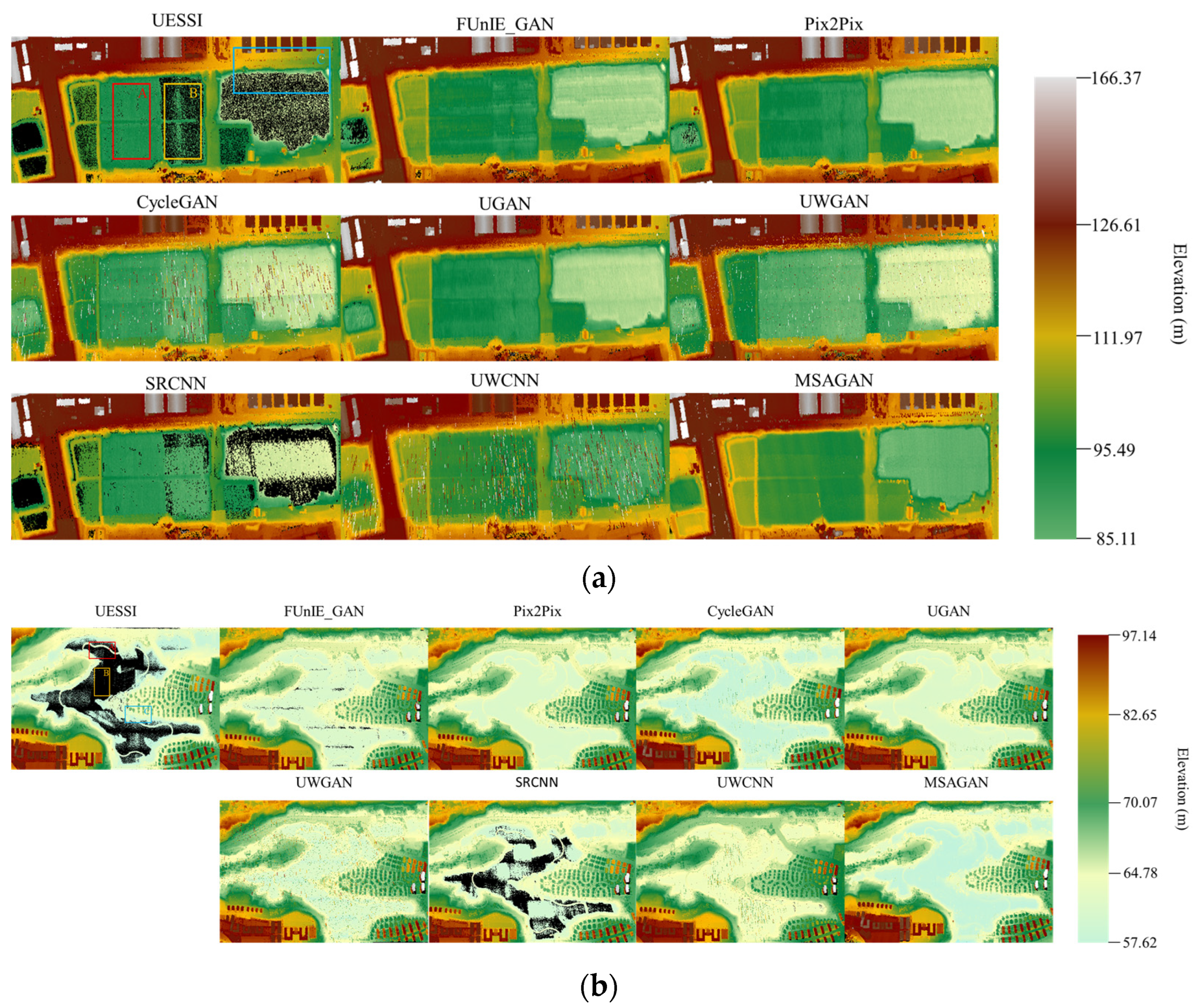
The center-of-mass shift in echo signal streak images during image enhancement is primarily caused by two factors: the generator fails to correctly enhance weak signal regions during the enhancement process, which results in non-rigid geometric deformation of the streaks, causing the center-of-mass to drift; and the generator fails to effectively constrain the pixel positions of valid echo signals during the enhancement process, leading to an overall translation of the streak image. L S p e c G r a d reduces the center-of-mass shift resulting from non-rigid morphological distortion by enforcing multi-scale structural and content alignment in the gradient domain; L W a v H F ensures consistency among the coefficients of the three frequency subbands in different directions, where each wavelet coefficient corresponds to gradient information along a specific direction within a local region of the image. This transforms sub-pixel shifts in weak echo signals into high-amplitude coefficient differences, generating a large loss gradient. Consequently, this loss function reduces the center-of-mass offset caused by rigid translation by penalizing spatial misalignment of high-frequency components and forcing the generated image to align with the real image in terms of details such as edges and textures. In streak images, the effective signal occupies only a tiny fraction of the pixels; pixel domain loss is easily dominated by the background, leading to discontinuities in the enhanced streak images. L C o n t r a applies discriminative separation between the effective echo signal region and the background region in the feature space, directly acting on feature similarity. It forces the model to bring positive sample pairs closer together in the latent space to maintain consistency in the streak content, while pushing negative sample pairs further apart to suppress background interference, thereby preventing the generation of discontinuous streaks.

4.2. Analysis of Point Cloud Authenticity in Reconstruction

In the raw underwater weak-echo streak images, although most signals are severely attenuated, some echoes still have a peak signal-to-noise ratio above the threshold and can be extracted and inverted to determine the three-dimensional coordinates of the detected targets. These points already exist in the raw data, represent actual underwater echo signals, and possess the system’s nominal detection accuracy. We selected 200 points as an internal reference benchmark to evaluate the reliability of the enhanced point cloud’s accuracy. Spatially associate the newly added points from the enhanced point cloud with the internal reference points. For each newly added point, search for its nearest neighbor among the reference points, calculate the elevation difference h between the two points, compute the distribution of h , and perform a Kolmogorov–Smirnov test comparing this distribution with the distribution of the closest elevation differences within the reference points themselves. The empirical cumulative distribution function (ECDF) plots for pond and lake are shown in Figure 15. The Kolmogorov–Smirnov test statistics D are 0.055 and 0.050, respectively, indicating that the distributions of the enhanced points and the reference points are similar; The p-values from the hypothesis test are 0.924 and 0.965, respectively. If p > 0.05, the null hypothesis cannot be rejected, indicating that the newly added point cloud is spatially statistically consistent with the true seabed echoes; they belong to the same continuous topographic surface rather than being isolated noise points.

4.3. Sensitivity Analysis of the Model to the Degree of Degradation

ASTIL’s echo streak images are fundamentally based on the spatial distribution of the laser spot on the target and the temporal broadening of the echo. Their skeletal structure is primarily determined by the target’s geometric shape. By treating strong-echo images of ground targets as an ideal domain, UESSI exhibits domain invariance in geometric shape mapping during the enhancement of underwater echo signals. Based on this property, MSAGAN separates structure from style, learning to extract domain-invariant geometric structures from weak underwater echo signals, and then learning the style of ground echoes characterized by minimal pulse broadening, high signal-to-noise ratio, and sharp, well-defined edges. Echo signals from the ground near the pond were acquired and degraded using the Jaffe-McGlamery model, sonar equation degradation, and Monte Carlo simulation, respectively, to simulate different underwater domains. The degradation parameters for each model are shown in Table 6. After enhancing the degraded streak images using MSAGAN, the resulting point cloud image is shown in Figure 16. By calculating the difference between the four vertices of each building in the degraded point cloud image and their corresponding points in the original point cloud image, and then taking the average, the values were 0.224 m, 0.243 m, and 0.317 m, respectively. The impact of domain gaps on point cloud accuracy is relatively small, indicating that the model exhibits a certain degree of robustness against parameterizable degradation factors such as intensity attenuation, noise, and broadening.

5. Conclusions

The proposed MSAGAN effectively addresses the key challenges in precisely enhancing underwater echo signal streak images based on original content, including the efficient extraction of original echo signal features, improved accuracy of streak image centroids, and reduced streak image fragmentation caused by background interference. MSAGAN integrates key components: Morphology-Aware Dynamic Receptive Field Attention, Spatial-Temporal Decoupled Frequency-Enhanced Global Feature Fusion Block, and Adaptive Dynamic Adjustment Loss Function Based on Frequency-Domain Decomposition and Gradient Response. It achieves effective and complete extraction of original echo signals with high-precision enhancement. While increasing the drift by only 0.0063, the 3D point cloud images of lakes and ponds saw point cloud increases of 3,095,864 and 578,804 respectively, the average point cloud density per square meter increased by 2.12 and 3.54 respectively, restoring more water body information. Moreover, it accurately identifies the echo characteristics of small target objects like trees with weak echo signals, effectively enhancing their echo signals while maintaining spatial 3D coordinates without displacement. Experimental results on our field-acquired dataset demonstrate that MSAGAN outperforms existing methods in several key metrics and enhanced image quality.

Author Contributions

Conceptualization, Q.Z. and Z.D.; methodology, Q.Z.; software, Q.Z.; validation, R.F., Z.D. and P.H.; formal analysis, Z.C.; investigation, Y.S. and W.L.; resources, R.F.; data curation, W.L.; writing—original draft preparation, Q.Z. and Z.D.; writing—review and editing, Z.D. and Z.C.; project administration, R.F.; funding acquisition, D.C. All authors have read and agreed to the published version of the manuscript.

Funding

This work was funded by the National Natural Science Foundation of China, with Grant No. 62305085 and No. 62192774, and the National Key Laboratory of Laser Spatial Information Foundation, with Grant No. LSI2026WDZC01.

Data Availability Statement

The data presented in this study are available on request from the corresponding author. The data are not publicly available due to funder regulations.
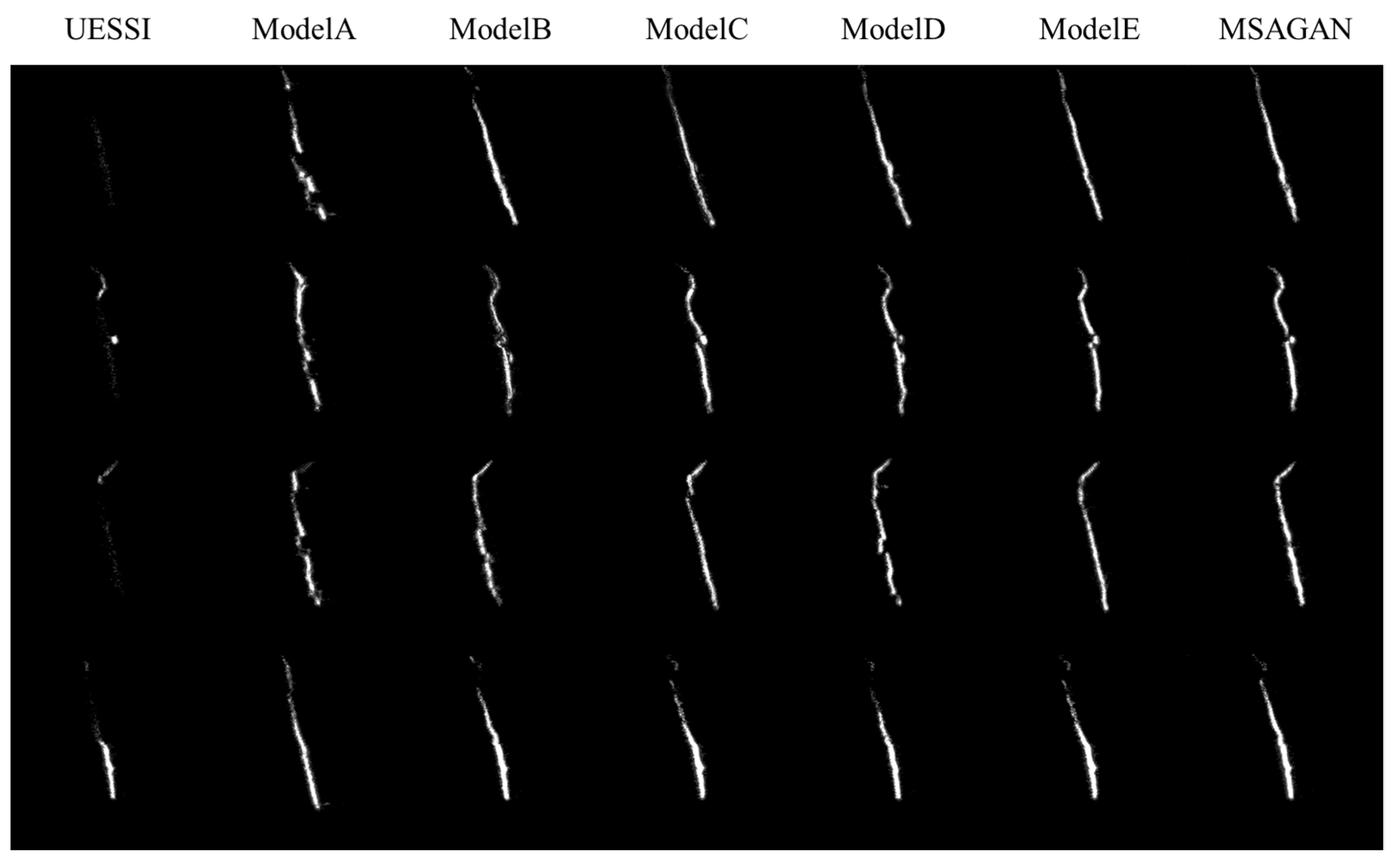
Conflicts of Interest

The authors declare no conflict of interest.

References

  1. Li, Z.P.; Huang, X.; Cao, Y.; Wang, B.; Li, Y.H.; Jin, W.; Yu, C.; Zhang, J.; Zhang, Q.; Peng, C.Z.; et al. Single-photon computational 3D imaging at 45 km. Photonics Res. 2020, 8, 1532–1540. [Google Scholar] [CrossRef]
  2. Chen, P.; Pan, D. Ocean optical profiling in South China Sea using airborne LiDAR. Remote Sens. 2019, 11, 1826. [Google Scholar] [CrossRef]
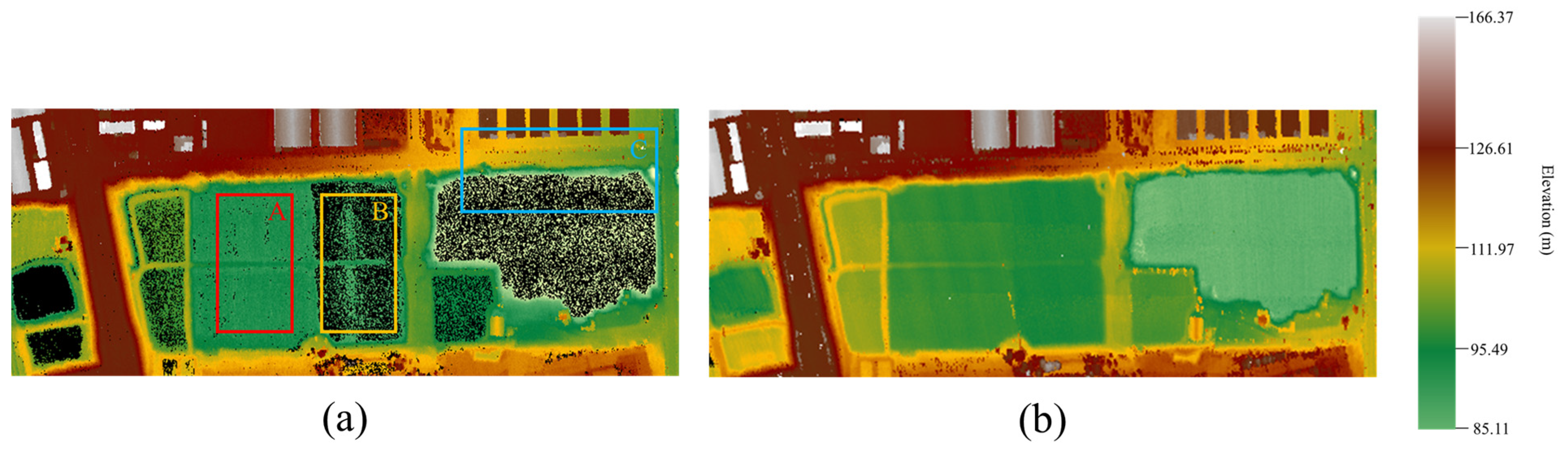
  3. Du, M.; Li, H.; Roshanianfard, A. Design and experimental study on an innovative UAV-LiDAR topographic mapping system for precision land levelling. Drones 2022, 6, 403. [Google Scholar] [CrossRef]
  4. Tian, Y.; Song, W.; Chen, L.; Fong, S.; Sung, Y.; Kwak, J. A 3D object recognition method from LiDAR point cloud based on USAE-BLS. IEEE Trans. Intell. Transp. Syst. 2022, 23, 15267–15277. [Google Scholar] [CrossRef]
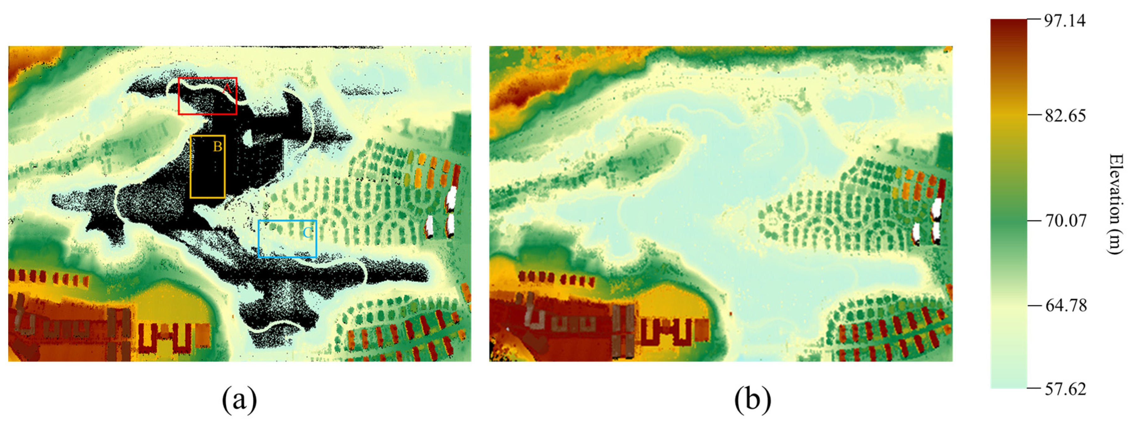
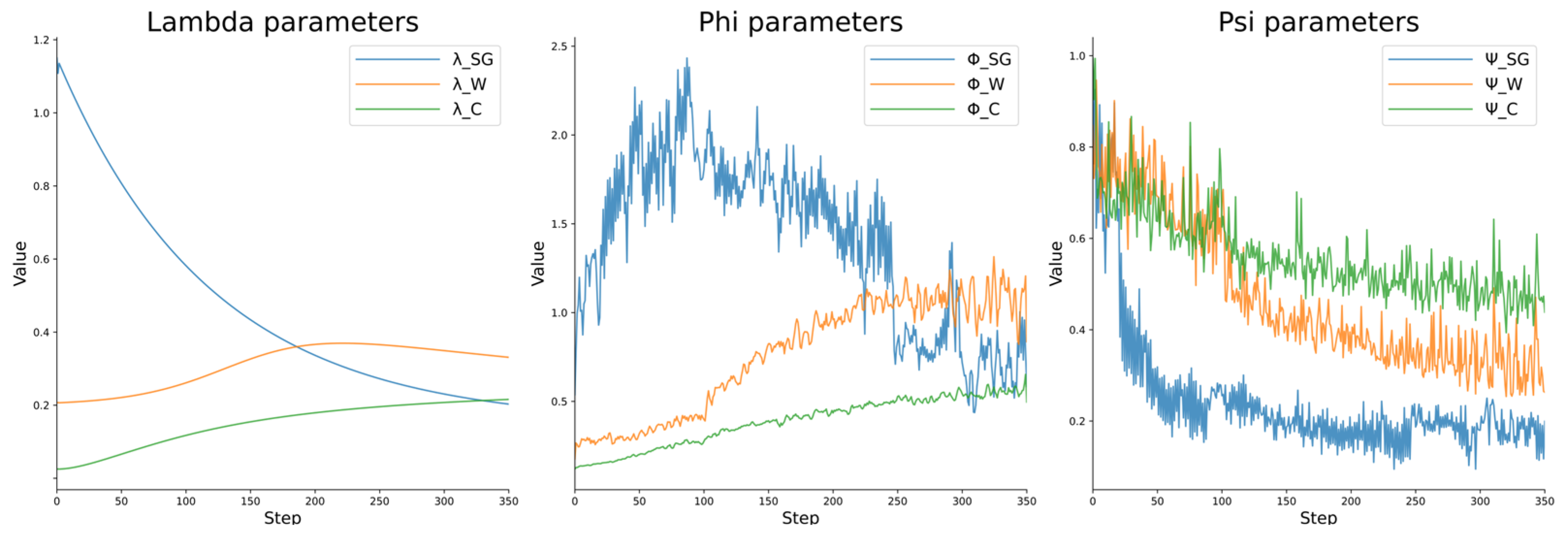
  5. Shen, H.; Dong, Z.; Yan, Y.; Fan, R.; Jiang, Y.; Chen, Z.; Chen, D. Building roof extraction from ASTIL echo images applying OSA-YOLOv5s. Appl. Opt. 2022, 61, 2923–2928. [Google Scholar] [CrossRef] [PubMed]
  6. Wu, L.; Gong, F.; Yang, X.; Xu, L.; Chen, S.; Zhang, Y.; Zhang, J.; Yang, C.; Zhang, W. The YOLO-based multi-pulse lidar (YMPL) for target detection in hazy weather. Opt. Lasers Eng. 2024, 177, 108131. [Google Scholar] [CrossRef]
  7. Dong, Z.; Yan, Y.; Jiang, Y.; Fan, R.; Chen, D. Ground target extraction using airborne streak tube imaging LiDAR. J. Appl. Remote Sens. 2021, 15, 016509. [Google Scholar] [CrossRef]
  8. Gao, J.; Sun, J.; Wei, J.; Wang, Q. Research of underwater target detection using a slit streak tube imaging lidar. In 2011 Academic International Symposium on Optoelectronics and Microelectronics Technology; IEEE: New York, NY, USA, 2011; pp. 240–243. [Google Scholar]
  9. Gao, J.; Sun, J.; Wang, Q. Experiments of ocean surface waves and underwater target detection imaging using a slit Streak Tube Imaging Lidar. Optik 2014, 125, 5199–5201. [Google Scholar] [CrossRef]
  10. Cui, Z.; Tian, Z.; Zhang, Y.; Bi, Z.; Yang, G.; Gu, E. Research on the underwater target imaging based on the streak tube laser lidar. In Young Scientists Forum 2017; SPIE: Bellingham, WA, USA, 2018; Volume 10710, pp. 838–844. [Google Scholar]
  11. Gao, J.; Sun, J.; Wang, Q.; Cong, M. 4-D imaging of the short scale ocean waves using a slit streak tube imaging Lidar. Optik 2017, 136, 136–143. [Google Scholar] [CrossRef]
  12. Fang, M.; Qiao, K.; Yin, F.; Xue, Y.; Tian, J.; Wang, X. Underwater 4D imaging quality enhancement of streak tube imaging LiDAR at extremely low SNR. Appl. Opt. 2025, 64, 3880–3889. [Google Scholar] [CrossRef] [PubMed]
  13. Fu, X.; Zhuang, P.; Huang, Y.; Liao, Y.; Zhang, X.P.; Ding, X. A retinex-based enhancing approach for single underwater image. In 2014 IEEE International Conference on Image Processing (ICIP); IEEE: New York, NY, USA, 2014; pp. 4572–4576. [Google Scholar]
  14. Wang, Y.; Song, W.; Fortino, G.; Qi, L.Z.; Zhang, W.; Liotta, A. An experimental-based review of image enhancement and image restoration methods for underwater imaging. IEEE Access 2019, 7, 140233–140251. [Google Scholar] [CrossRef]
  15. Peng, Y.T.; Chen, Y.R.; Chen, Z.; Wang, J.H.; Huang, S.C. Underwater image enhancement based on histogram-equalization approximation using physics-based dichromatic modeling. Sensors 2022, 22, 2168. [Google Scholar] [CrossRef] [PubMed]
  16. Song, W.; Wang, Y.; Huang, D.; Liotta, A.; Perra, C. Enhancement of underwater images with statistical model of background light and optimization of transmission map. IEEE Trans. Broadcast. 2020, 66, 153–169. [Google Scholar] [CrossRef]
  17. Berman, D.; Levy, D.; Avidan, S.; Treibitz, T. Underwater single image color restoration using haze-lines and a new quantitative dataset. IEEE Trans. Pattern Anal. Mach. Intell. 2021, 43, 2822–2837. [Google Scholar] [CrossRef] [PubMed]
  18. Galdran, A.; Pardo, D.; Picón, A.; Alvarez-Gila, A. Automatic red-channel underwater image restoration. J. Vis. Commun. Image Represent. 2015, 26, 132–145. [Google Scholar] [CrossRef]
  19. Dong, C.; Loy, C.C.; He, K.; Tang, X. Image super-resolution using deep convolutional networks. IEEE Trans. Pattern Anal. Mach. Intell. 2015, 38, 295–307. [Google Scholar] [CrossRef] [PubMed]
  20. Li, C.; Anwar, S.; Porikli, F. Underwater scene prior inspired deep underwater image and video enhancement. Pattern Recognit. 2020, 98, 107038. [Google Scholar] [CrossRef]
  21. Isola, P.; Zhu, J.Y.; Zhou, T.; Efros, A.A. Image-to-image translation with conditional adversarial networks. In Proceedings of the IEEE Conference on Computer Vision and Pattern Recognition; IEEE: New York, NY, USA, 2017; pp. 1125–1134. [Google Scholar]
  22. Zhu, J.Y.; Park, T.; Isola, P.; Efros, A.A. Unpaired image-to-image translation using cycle-consistent adversarial networks. In Proceedings of the IEEE International Conference on Computer Vision; IEEE: New York, NY, USA, 2017; pp. 2223–2232. [Google Scholar]
  23. Islam, M.J.; Xia, Y.; Sattar, J. Fast underwater image enhancement for improved visual perception. IEEE Robot. Autom. Lett. 2020, 5, 3227–3234. [Google Scholar] [CrossRef]
  24. Fabbri, C.; Islam, M.J.; Sattar, J. Enhancing underwater imagery using generative adversarial networks. In 2018 IEEE International Conference on Robotics and Automation (ICRA); IEEE: New York, NY, USA, 2018; pp. 7159–7165. [Google Scholar]
  25. Wang, N.; Zhou, Y.; Han, F.; Zhu, H.; Yao, J. UWGAN: Underwater GAN for real-world underwater color restoration and dehazing. arXiv 2019, arXiv:1912.10269. [Google Scholar]
  26. Chen, Z.; Shao, F.; Fan, Z.; Wang, X.; Dong, C.; Dong, Z.; Fan, R.; Chen, D. A Calibration Method for Time Dimension and Space Dimension of Streak Tube Imaging Lidar. Appl. Sci. 2023, 13, 10042. [Google Scholar] [CrossRef]
  27. Yan, Y.; Wang, H.; Song, B.; Chen, Z.; Fan, R.; Chen, D.; Dong, Z. Airborne streak tube imaging LiDAR processing system: A single echo fast target extraction implementation. Remote Sens. 2023, 15, 1128. [Google Scholar] [CrossRef]
  28. Yan, Y.; Wang, H.; Dong, Z.; Chen, Z.; Fan, R. Extracting suburban residential building zone from airborne streak tube imaging LiDAR data. Measurement 2022, 199, 111488. [Google Scholar] [CrossRef]
  29. Mao, X.; Li, Q.; Xie, H.; Lau, R.Y.; Wang, Z.; Paul Smolley, S. Least squares generative adversarial networks. In Proceedings of the IEEE International Conference on Computer Vision; IEEE: New York, NY, USA, 2017; pp. 2794–2802. [Google Scholar]
  30. Li, X.; Zhou, Y.; Xu, H.; Lu, W.; Fan, R.; Chen, D.; Jiang, Y.; Yan, R. High-stability, high-pulse-energy MOPA laser system based on composite Nd: YAG crystal with multiple doping concentrations. Opt. Laser Technol. 2022, 152, 108080. [Google Scholar] [CrossRef]
  31. Zhang, R.; Isola, P.; Efros, A.A.; Shechtman, E.; Wang, O. The unreasonable effectiveness of deep features as a perceptual metric. In Proceedings of the IEEE Conference on Computer Vision and Pattern Recognition; IEEE: New York, NY, USA, 2018; pp. 586–595. [Google Scholar]
  32. Li, W.; Guo, S.; Zhai, Y.; Liu, F.; Lai, Z.; Han, S. Target classification of multislit streak tube imaging lidar based on deep learning. Appl. Opt. 2021, 60, 8809–8817. [Google Scholar] [CrossRef] [PubMed]
  33. Wang, X.; Chen, Z.; Dong, C.; Dong, Z.; Fan, R.; Hao, P.; Chen, D. Presegmentation of Point Cloud Based on Centroid Matrix of Streak Tube Imaging LiDAR. IEEE Geosci. Remote Sens. Lett. 2025, 22, 6500404. [Google Scholar] [CrossRef]
  34. Wang, X.; Chen, Z.; Dong, C.; Dong, Z.; Chen, D.; Fan, R. High accuracy reconstruction of airborne streak tube imaging LiDAR using particle swarm optimization. Appl. Sci. 2024, 14, 6843. [Google Scholar] [CrossRef]
  35. Wei, Z.; Long, J.; Zhang, Z.; Xue, X.; Sun, Y.; Li, Q.; Liu, W.; Shen, J.; Zhang, Z.; Li, X.; et al. Structure-aware completion of plant 3D LiDAR point clouds via a multi-resolution GAN-inversion network. Front. Plant Sci. 2025, 16, 1698843. [Google Scholar] [CrossRef] [PubMed]
Figure 1. ASTIL Scanning Mode.
Remotesensing 18 02689 g001
Figure 2. Structure of streak tube imaging unit.
Remotesensing 18 02689 g002
Figure 3. Schematic Diagram of Morphology-Aware Dynamic Receptive Field Attention.
Remotesensing 18 02689 g003
Figure 4. Schematic Diagram of Spatial-Temporal Decoupled Frequency-Enhanced Global Feature Fusion Block.
Remotesensing 18 02689 g004
Figure 5. Schematic Diagram of the MSAGAN Generator Network Architecture.
Remotesensing 18 02689 g005
Figure 6. Coordinate transformation in point cloud inversion process.
Remotesensing 18 02689 g006
Figure 7. Satellite imagery of the pond detection area.
Remotesensing 18 02689 g007
Figure 8. Satellite imagery of the lake detection area.
Remotesensing 18 02689 g008
Figure 9. Enhanced Effect Diagram of the UESSI Model Comparison.
Remotesensing 18 02689 g009
Figure 10. (a) 3D point cloud images generated by enhancing the streak images of pond echo signals using various neural network models; (b) 3D point cloud images generated by enhancing lake echo signal streak images using various neural network models.
Remotesensing 18 02689 g010
Figure 11. Comparison of MSAGAN’s Performance Improvements Under Different Module Configurations.
Remotesensing 18 02689 g011
Figure 12. (a) Raw pond underwater echo signal streak image, point cloud image; (b) Enhanced pond underwater echo signal streak image, point cloud image.
Remotesensing 18 02689 g012
Figure 13. (a) Raw lake underwater echo signal streak image, point cloud image; (b) Enhanced lake underwater echo signal streak image, point cloud image.
Remotesensing 18 02689 g013
Figure 14. Schematic Diagram of Dynamic Adjustment of GL-DAM Parameters.
Remotesensing 18 02689 g014
Figure 15. (a) pond Empirical cumulative distribution function; (b) lake empirical cumulative distribution.
Remotesensing 18 02689 g015
Figure 16. Point cloud image of the original ground echo and various degradation models.
Remotesensing 18 02689 g016
Table 1. Details of the various datasets.
Echo Signal TypesTotal NumberTraining SetTest Set
UESSI398229711011
GESSI10,26687641502
Table 2. Comparative Model Evaluation Results.
MethodPSNRSSIMLPIPSCMD
FUnIEGAN25.07870.97320.06350.0102
Pix2Pix27.74960.97460.04860.0097
CycleGAN24.82450.96450.06590.0121
UGAN26.62360.97280.05270.0108
UWGAN24.19630.95710.11710.0362
SRCNN27.43150.98840.04020.0027
UWCNN25.75040.96770.06130.0107
MSAGAN27.86350.98240.04170.0063
Table 3. Average elevation of point cloud images generated from underwater echo signals.
Average Elevation of the Water Area ( m )
UESSIFUnIGPix2PixCycleUGAUWGSRCUWCMSAG
Pond65.43763.30663.07561.69462.93058.08665.19063.12865.184
Lake86.13884.39684.55283.05683.46079.02886.01083.71085.897
Table 4. Evaluation Results of Ablation Study.
MethodComponentsEvaluation Metric
BaseMADRASTDFBlockFGADPSNRSSIMLPIPSCMD
ModelA 24.39720.96880.13310.0261
ModelB 25.57360.97320.07850.0174
ModelC 25.86310.97890.06930.0107
ModelD 26.52420.97530.06550.0128
ModelE 27.32400.98020.05480.0059
MSAG27.86350.98240.04170.0063
Table 5. Point Cloud Density Before and After Enhancement.
RegionOriginal Point Cloud Density ( m 2 ) Enhanced Point Cloud Density ( m 2 )
SWZoneDWZoneSWZoneDWZone
Pond2.000.243.033.42
Lake0.440.0683.973.67
Table 6. Parameter settings for each degradation model.
ParameterJaffe-McGlamerySonar EquationMonte Carlo
Attenuation coefficient (m−1)0.080.040.05
Target distance (m)15.010.08.0
Backscatter300.10.2
Pulse spread sigma (pixels)1.20.5
SNR (dB)4540
PSF size (pixels)15
Number of photons50,000
Anisotropy factor g0.7
Scattering coefficient (m−1)0.3
Absorption coefficient (m−1)0.06
Maximum propagation distance (m)10
Disclaimer/Publisher’s Note: The statements, opinions and data contained in all publications are solely those of the individual author(s) and contributor(s) and not of MDPI and/or the editor(s). MDPI and/or the editor(s) disclaim responsibility for any injury to people or property resulting from any ideas, methods, instructions or products referred to in the content.