


Highlights
What are the main findings?
- Proposed VDCnet, a view-consistent domain calibration network that improves single-source cross-scene HSI classification through calibrated domain expansion and view semantic matching.
- Demonstrated that calibrated spectral-spatial perturbation and multi-view semantic consistency can effectively reduce semantic drift under unseen scene shifts, achieving up to a 2.65-percentage-point OA improvement over advanced DG methods.
What are the implications of the main finding?
- The proposed method provides a more reliable solution for cross-scene HSI classification by enhancing sample diversity while suppressing the risk of semantic drift in generated samples.
- The combination of calibrated spectral-spatial perturbation and multi-view semantic consistency offers a generalizable paradigm for remote sensing domain generalization under unseen scene shifts.
Abstract
Cross-scene hyperspectral image (HSI) classification seeks to learn a classifier from annotated source-scene data and deploy it on unlabeled scenes whose imaging conditions and data distributions differ from those seen during training. Existing cross-scene learning strategies mainly include domain adaptation (DA) and domain generalization (DG). In practical scenarios, target-domain samples are commonly unknown, inaccessible, or time-varying before deployment. DG is a more practical choice for such applications. Yet, single-source DG still faces a key difficulty: expanded samples must contain meaningful domain changes without corrupting class semantics. If the generated domains are weak or deviate from their original categories, the classifier may learn unstable or misleading cues. Therefore, we introduce the View-Consistent Domain Calibration Network (VDCnet), which is designed to improve the quality and training value of generated samples for single-source cross-scene classification. VDCnet consists of a Calibrated Expansion Generator (CEG) and a View Semantic Matching Mechanism (VSM). CEG performs reliability-gated spectral-spatial residual perturbation to produce semantically trustworthy extended samples, rather than simply enlarging the sample set. VSM further enforces multi-view semantic consistency in both prediction distributions and projected feature representations, promoting diverse feature learning while suppressing semantic drift. Experiments on the Houston, Pavia, and Shanghai–Hangzhou datasets demonstrate that VDCnet improves overall accuracy over the leading DG methods by 1.29, 2.65, and 1.26 percentage points, respectively, indicating its superior performance.
1. Introduction
Hyperspectral remote sensing technology uses imaging spectrometers to acquire data across hundreds of continuous and adjacent spectral channels, which usually cover the visible to near-infrared spectrum and provide detailed spectral information for ground objects [1,2,3]. Hyperspectral image classification seeks to categorize each pixel into a designated land-cover class based on its spectral-spatial characteristics. As a fundamental task in hyperspectral remote sensing interpretation, HSI classification is crucial for reliable land-cover information extraction [4,5] and has been widely applied to urban environmental planning [6], pollution monitoring [7], precision agriculture [8], and geological and mineral exploration [9].
The rapid development of deep learning has substantially advanced hyperspectral image classification, with classification accuracy continuing to improve [10,11,12,13,14]. However, most deep-learning-based HSI classification methods rely on sufficient labeled samples, whereas manual annotation is labor-intensive and costly. This limitation has made cross-scene classification an increasingly important research topic. Cross-scene classification seeks to train a model utilizing labeled source-domain data (SD) to proficiently classify unlabeled target-domain data (TD) from different scenes [15]. However, the SD and TD usually differ in imaging sensors, imaging conditions, and land-cover distributions, which induces significant domain shifts between the two domains. As a result, the classification accuracy on the TD decreases significantly, resulting in significant performance deterioration during direct SD-to-TD transfer [16,17].
Domain adaptation (DA) methods address the issues by reducing the domain bias during training and learning feature representations that are insensitive to domain variations [18,19,20]. Qin et al. [21] aligned source–target subspaces by jointly learning alignment and projection matrices within a Tucker decomposition framework, while preserving spatial–spectral multilinear structures of tensorized HSIs. Tang et al. [22] achieved end-to-end domain- and class-level feature alignment through domain adversarial and biclassifier adversarial modules. Gao et al. [23] guided pseudo-label optimization with estimated target pseudo-class distributions, formulated label correction as a zero–one programming problem, and used a frequency-domain phase view to extract domain-stable features. Although domain adaptation methods can mitigate the decline in cross-domain classification performance caused by domain shift, their training phase relies on accessible target domain samples. In practical applications, however, target scenes are often difficult to obtain in advance or may change frequently, making it challenging to meet practical application needs [24,25].
In recent years, domain generalization (DG) has emerged as another cross-scene learning paradigm that does not rely on TD data. DG learns predictive models solely from labeled SD data and enables their generalization to unseen TDs without access to TD data during training [26,27,28]. DG approaches for cross-scene HSI classification generally follow two main directions: one focuses on source domain expansion and data augmentation, enhancing the model’s coverage of unknown target domains by constructing diverse simulated extended domains [29,30]. The other category focuses on domain-invariant representation learning, driving the model to capture cross-domain stable discriminative features by introducing cross-modal prior knowledge or explicit constraints on feature distribution structures [31,32]. Compared with domain-invariant representation learning, source-domain-expansion-based methods can directly enrich the accessible training distribution by constructing extended domains from limited labeled SD samples, making them widely used in single-source DG. However, existing source-domain expansion methods mainly emphasize the diversity of generated samples, while the semantic reliability of each generated view is still insufficiently calibrated. For example, SDEnet [29] randomizes spatial and spectral features to enlarge the source distribution, but separate randomization may weaken their intrinsic coupling. Moreover, classification supervision alone cannot fully constrain the semantic consistency among generated views. This motivates VDCnet to combine reliability-gated spectral-spatial expansion with multi-view semantic matching.
To address these challenges, we propose the View-Consistent Domain Calibration Network (VDCnet). Through CEG, VDCnet introduces gated spectral-spatial residual perturbations to construct semantically reliable extended-domain and intermediate-domain samples; it then employs VSM to establish a multi-view semantic consistency constraint, enabling the model to enhance SD neighborhood coverage while maintaining stable class semantics, thus improving its cross-scene generalization ability.
The contributions of this work are threefold.
- We propose CEG to generate extended-domain samples through reliability-gated spectral-spatial residual perturbations. Different from separate spatial or spectral randomization, CEG calibrates perturbations at both channel and spatial locations to better preserve HSI class semantics.
- We propose VSM to constrain generated views through multi-view semantic matching. It uses reliability-weighted classification, projected-feature consistency, and class-consensus consistency to reduce semantic drift during source-domain expansion.
- We integrate CEG and VSM into VDCnet for single-source cross-scene HSI classification. The framework improves source-neighborhood coverage during training while retaining a single-branch classifier for target-domain inference.
1.1. Domain Generalization
Domain generalization (DG) trains models on one or multiple source domains and enables their application to unseen target domains without access to target-domain samples. Unlike domain adaptation, which requires TD samples for training or alignment, DG is more suitable for scenarios where TD data are difficult to obtain, costly to collect, or highly dynamic. Based on the number of source domains involved, DG is commonly classified into single-source domain generalization (SDG) and multi-source domain generalization (MDG): SDG uses only one labeled source scene and requires fewer data but provides limited learnable cross-domain variations [33,34], while MDG uses multiple SD to obtain more stable domain-invariant features but requires labeled multi-scene data [35,36]. In hyperspectral image classification, the high cost of labeled samples and limited source scenes make SDG more practical, and existing DG methods mainly follow two pathways: source-domain-expansion-based methods and domain-invariant representation learning methods.
Source-domain-expansion-based DG methods enhance generalization by increasing data diversity. Through techniques such as style transfer, adversarial perturbation, and feature-space interpolation, they synthesize virtual samples with distributional variations from limited SD data, thereby expanding the accessible training distribution and improving the model’s coverage of unseen TD during inference. Zhang et al. [29] developed a Single-source Domain Expansion Network that employs semantic and morph encoders to perform spatial and spectral randomization on source samples and learns class-wise domain-invariant representations through supervised contrastive adversarial learning. Dong et al. [30] introduced a spatial–spectral enhancement and causal constraint network, which generates spectral and spatial enhanced domains via AdaIN and STN and derives potential causal invariant features based on a structural causal model.
Domain-invariant representation learning methods emphasize cross-domain feature stability. By imposing intraclass consistency constraints, introducing cross-modal spectral priors, or constructing explicit distribution alignment objectives, these methods suppress domain-specific styles and preserve land-cover discriminability, thereby improving generalization to unseen target scenes. Zhang et al. [31] proposed a language-guided framework that uses coarse- and fine-grained textual descriptions of land-cover classes to construct a shared semantic space across domains, and obtains domain-invariant class representations via supervised contrastive alignment between visual and linguistic features. Qin et al. [32] proposed a Frequency Disentanglement and Data Geometry Constraint Network that disentangles semantic high-frequency and stylistic low-frequency components to simulate controllable domain gaps and constrains extended domains within reasonable support through data geometry constraints.
Recently, DG for HSI classification has increasingly focused on generalized modeling with stronger structural constraints and greater representational capacity. Huang et al. [37] learned dynamic attention maps in frequency space to filter generalizable frequency components and used balanced attentional consistency based on class activation maps to improve the reliability of generated samples. Gao et al. [38] used feature style covariance for finer style–content randomization and employed a spatial shuffling discriminator to reduce the interference of intrinsic spatial structures with invariant semantic learning. Jin et al. [39] employed a language-guided dual-branch Mamba to model spatial and spectral features with Mamba-based scanning, and strengthened domain-invariant representation learning by generating label- and text-derived prior knowledge for contrastive learning.
1.2. Feature Diversification with Semantic Preservation
Hyperspectral images contain rich and continuous spatio-spectral information, providing abundant transferable features for cross-scene classification. Based on this characteristic, early SDG methods typically enhanced SD diversity by constructing extended domains. Zhao et al. [40] employed locally linear unbiased randomization to generate style-varied extended samples, and combined supervised contrastive learning with adversarial inter- and intra-class contrastive regularization to learn domain-invariant representations. Chen et al. [41] designed a Spectral–Spatial Adversarial Multidomain Synthetic Network, which synthesizes diverse generative domains via dual spectral–spatial domain-generation networks and uses mutual information regularization to preserve class-level semantic consistency. However, such methods place greater emphasis on increasing the variability of the extended domain, and the generated samples may still deviate from the original semantics in terms of spectral response or spatial structure, leading to the introduction of unreliable supervision during the enhancement process.
To address the above problems, subsequent studies have gradually turned to constrained expansion with semantic reliability. Peng et al. [42] employed Transformer-based style transfer to expand the SD distribution, and progressively disentangled domain-invariant and domain-specific features to reduce the interference of style perturbations with class-discriminative information. Huang et al. [43] adopted progressive adversarial domain augmentation to generate extended samples, introduced richer domain variations through a domain-aware spatial–spectral mask, and further used a two-level contrastive constraint to prevent augmented features from deviating from class semantics. Chen et al. [44] designed spectral property-driven data augmentation based on hyperspectral channel variation and adjacent-channel mixing, which expands spectral feature distributions while using spatial–spectral collaborative constraints to suppress unrealistic perturbations from damaging semantic structures.
However, existing methods primarily establish constraints around a single extended domain or specific augmentation forms, making it difficult to fully capture the continuous semantic relationships among the source domain, extended domains, inter-domain transition samples, and frequency-enhanced views. Additionally, the reliability of augmented samples lacks sample-level adaptive evaluation, and samples with semantic drift may introduce noise into the supervision. Therefore, we propose VDCnet: on the one hand, it utilizes CEG to construct controlled extended domain and intermediate domain samples, thereby expanding the SD neighborhood coverage; on the other hand, it employs VSM to establish multi-view semantic consistency constraints, which enhance feature diversity while reducing the risk of generated samples deviating from the original class semantics.
2. Materials and Methods
As shown in Figure 1, VDCnet improves the utility of generated extended-domain samples for single-source cross-scene HSI classification. It comprises CEG and VSM. CEG generates extended- and intermediate-domain views through gated spectral–spatial residual perturbations, while VSM enforces multi-view semantic consistency across the three base views and their frequency-enhanced counterparts using classification predictions, projected features, and class consensus. During training, the shared feature extractor, classification head, and projection head are jointly optimized. During testing, only the feature extractor and classification head are retained for TD classification.
Figure 1.
Overall framework of VDCnet. During training, CEG takes the SD sample as input and generates the ED sample ; the ID sample is then constructed from and . The three base views are further processed by frequency enhancement to form the six-view set . The six views are fed into the shared feature extractor ; the classification head outputs classification logits, and the projection head generates normalized projected features. The model is jointly optimized using the reliability-weighted classification loss , the supervised contrastive consistency loss , and the sample-pair class-consensus consistency loss . During testing, the TD sample is classified only by the trained and .
2.1. Problem Definition
Given a labeled SD dataset
where denotes the ith hyperspectral local sample, is its class label, and C, H, W, and N denote the numbers of spectral channels, sample height, sample width, and classes, respectively. The TD dataset is denoted by
The TD shares the same feature and label spaces as the SD but is inaccessible during training. Because imaging conditions and land-cover distributions vary across scenes, the source and target domains usually follow different joint distributions:
The goal of SDG is therefore to learn, from alone, a classification function consisting of a feature extractor and a classification head :
where ∘ denotes function composition. The learned classifier is expected to generalize across scenes without accessing TD training samples.
2.2. Calibrated Expansion Generator
The Calibrated Expansion Generator (CEG) constructs extended-domain samples around the SD while preserving class semantics. It first generates candidate spectral-spatial residuals with fixed Gaussian-smoothed 3D random convolution blocks; subsequently, unreliable perturbations are suppressed through a spectral-spatial reliability gate; then, the residual strength is adjusted using a curriculum perturbation schedule. Given a mini-batch of SD samples , CEG produces the extended-domain samples as
B, C, H, and W denote the batch size, spectral-channel number, patch height, and patch width, respectively.
2.2.1. Spectral-Spatial Random Residual Generation
The process for generating candidate spectral-spatial random residuals is illustrated in Figure 2. To simulate complex but locally continuous changes in spectral-spatial responses across scenes, CEG first lifts the input samples into five-dimensional tensors
The channel dimension C provides the input channels for the 3D convolution, and the added depth dimension is fixed at 1 to match the Conv3D format. Thus, the random convolution block updates the internal perturbation tensor through layer-wise spectral-spatial responses. For the lth block, the random convolution response tensor is first computed as
where denotes the input perturbation tensor of the lth block, denotes the corresponding intermediate random response, ∗ denotes 3D convolution, and and denote the fixed random convolution kernel and random bias term.
where denotes the randomly initialized weights, and ⊙ denotes element-wise multiplication. This design retains the diversity of random perturbations while introducing a locality prior into the convolution kernel. The mask is computed from the position coordinates within the convolution kernel and the scale parameter :
Here, controls the smoothing range of the Gaussian mask, and the denominator keeps the average scale of the mask stable. This mask smoothly constrains the random convolution kernel within local neighborhoods, making the generated random responses better preserve local structural continuity. By emphasizing nearby positions and attenuating distant responses, it reduces abrupt structural perturbations that may damage class semantics. The features obtained after the random convolution are then processed by in-sample normalization and a bounded nonlinear mapping:
In the normalization term, and are the mean and standard deviation of over the depth and spatial dimensions, respectively; is used for numerical stability; and and are fixed stochastic affine modulation parameters. To reduce computational cost and preserve the locality of spectral perturbations, the random 3D convolution and subsequent channel reshaping use grouped convolution compatible with the number of spectral channels.
Figure 2.
Mechanism of candidate spectral-spatial random residual generation.
At training epoch , the number of active random 3D convolution blocks is
denotes the total number of random convolutional blocks, limits the maximum activation depth, and I is the interval for increasing the active depth. In each forward pass, only the first random 3D convolution blocks are used to update the perturbation tensor. After these blocks, CEG squeezes the auxiliary depth dimension and applies one grouped Conv2D followed by batch normalization and tanh to refine the residual:
2.2.2. Reliability-Gated Calibration
Random residuals introduce spatial variation, but different channels and spatial locations do not require the same perturbation strength. CEG therefore introduces a spectral-spatial reliability gate to adaptively calibrate the residuals. First, average pooling and max pooling are applied to the candidate perturbed samples along the spatial dimensions, and the channel gate is obtained through two convolutional layers:
Next, average pooling and max pooling are applied to along the spectral-channel dimension, and the spatial gate is obtained through a convolution:
denotes concatenation, while and denote average pooling and max pooling, respectively. Combining the channel and spatial reliability gates yields the gating matrix
where ⊗ denotes element-wise multiplication. The final ED samples are obtained by adding the gated residual to the SD sample:
where is a learnable residual scaling factor, and r is a trainable scalar optimized end-to-end. In contrast, is a deterministic epoch-dependent perturbation strength computed from the predefined schedule hyperparameters. By suppressing random perturbations in low-confidence regions, this gating mechanism encourages CEG to generate ED samples that better preserve class semantics.
2.2.3. Curriculum Perturbation Scheduling
Early training benefits from stronger domain expansion because it increases sample diversity, whereas persistent strong perturbations in later training may cause the classification network to overfit generated patterns. CEG therefore adopts a curriculum perturbation schedule. Its cosine annealing form is
, , and specify the initial perturbation strength, the final perturbation strength after annealing, and the perturbation upper bound, respectively; and are the start and end epochs of annealing. This strategy provides sufficient domain expansion in early training and gradually weakens perturbations in later stages, reducing the model’s reliance on strong random perturbation patterns.
2.3. View Semantic Matching Mechanism
Although CEG broadens the SD distribution, generated samples may still suffer from semantic drift in local texture, spectral response, or frequency-domain structure. The View Semantic Matching Mechanism (VSM) builds a six-view semantic matching framework around the source-domain view , the extended-domain view , the intermediate-domain view , and their frequency-enhanced counterparts , , and . It constrains generated samples through reliability-weighted classification supervision, projected-feature consistency, and sample-pair class-consensus consistency, guiding the model to learn class-relevant rather than domain-specific representations. VSM consists of a shared feature extractor , a classification head , and a projection head . The feature extractor stacks three Conv2D-ReLU blocks to extract deep features; uses global average pooling and a linear classifier to output classification logits; and maps pooled features to normalized projected features to constrain multi-view class geometry in the normalized projection space.
2.3.1. Multi-View Construction
Given an SD view , CEG generates an ED view
To enhance continuous domain coverage between the source and extended domains, an intermediate-domain view is further constructed as
The mixing coefficient is randomly sampled. As a convex mixture of and , lies between the source and extended domains and helps alleviate the insufficient cross-domain transition caused by training only on discrete domain views.
Frequency-enhanced views are then created for , , and to simulate global spectral-spatial response variations caused by sensor response, illumination changes, and scene-background differences. For each view X, a two-dimensional Fourier transform is independently performed on each spectral channel:
Let
where A and represent the amplitude and phase spectra. Amplitude perturbations mainly alter the frequency-energy distribution, whereas phase perturbations affect spatial structure; both are therefore subject to constrained random perturbations:
The perturbation variables satisfy and . The variable a is restricted to a neighborhood of 1, and b introduces only small random perturbations, keeping the amplitude and phase spectra within a controlled range and preventing excessive changes in the frequency-domain response. The frequency-enhanced view is finally obtained through the inverse Fourier transform:
This operation maps , , and to , , and , respectively. The subscripts denote the base views, and the superscript f denotes their frequency-enhanced counterparts.
The six-view set during training is defined as
2.3.2. Reliability-Weighted Classification Supervision
The classification loss encourages each view to maintain correct label discriminability. For any view , the shared feature extractor, classification head, and softmax probability are defined as
where denotes the classification logits, and denotes the class probability distribution. The SD view provides the most reliable semantic anchor. The reliability of each generated view is estimated from its true-class confidence and its prediction-distribution consistency with the SD view. For the generated view v of the ith sample, the reliability weight is defined as
In the reliability term, and are the predicted distributions of the SD view and view v, respectively; is the predicted probability assigned by view v to the true class ; and is the lower weight bound. If a generated view has low confidence in the true class or its prediction distribution deviates substantially from that of the SD view, is reduced accordingly. This weight is detached from backpropagation and serves only as a sample-level loss coefficient.
The reliability-weighted classification loss is
Here, indexes a mini-batch sample, s denotes the SD view, and v indexes a view in . is the sample-wise cross-entropy loss, is the detached reliability weight, and is a small constant for numerical stability. Thus, the first term is the mean loss of the reliable SD anchor, whereas the second is the reliability-normalized weighted mean over the five non-source views. When reliability weighting is disabled, the implementation instead uses the unweighted mean of the classification losses over all six views.
2.3.3. Projected-Feature Consistency
Here, feature geometry refers to the pairwise angular relationships among -normalized projected features, characterized by within-class compactness and between-class separation. Supervised classification constrains predictions but does not explicitly organize these relationships, as views with the same predicted label may remain distant and retain scene-specific cues. VSM therefore introduces supervised contrastive consistency in the normalized projection space, attracting same-class projections across samples and views while separating projections from different classes. This forms a class-discriminative feature geometry that remains stable across the six view transformations. For each view, GAP first converts into a pooled feature vector, which is then mapped by the projection head and -normalized:
Specifically, each feature map is first transformed into a vector by GAP and then mapped through a projection head shared across all six views. The output is -normalized to obtain the projected feature , which is used only to compute during training. Let denote the mth view projection of the ith sample in a batch, and denote its class label. For an anchor , the set of positive samples is defined as
The supervised contrastive consistency loss is defined as
is the contrastive temperature. This loss preserves intraclass feature compactness under multi-view perturbations, helping the model extract class-discriminative representations that are insensitive to domain changes.
2.3.4. Sample-Pair Class-Consensus Consistency
This loss further constrains prediction-distribution consistency between each base view and its frequency-enhanced counterpart. For paired views , namely , , and , let denote the index set of samples from class c in the batch. Class consensus is computed only for classes with in the current batch; absent classes do not participate in consensus construction. The class-consensus logits are defined as
For a sample with label , the distillation target is . Let
where T is the distillation temperature. Gradients are stopped through the class-consensus logits in the distillation target, which serves as the teacher distribution for constraining the paired views. The class-consensus consistency term for one paired-view set is
For the three paired-view sets, the sample-pair class-consensus consistency loss is weighted by the average reliability of the corresponding frequency-enhanced views:
The batch-level average reliabilities of the corresponding frequency-enhanced views are denoted by , , and . If reliability weighting is disabled, the three paired losses are simply averaged. Because the classification network has not yet formed stable predictions in the early training stage, the class-consensus constraint is enabled only after the warm-up epochs to reduce interference from erroneous early consensus.
2.4. Optimization Objective and Inference
During training, CEG constructs the ED and ID views. The six views share , , and and are optimized using the multi-view joint objective
and regulate the effect of the supervised contrastive consistency loss and the sample-pair class-consensus consistency loss, respectively. Each training iteration first processes the SD sample through CEG to obtain an ED view and then linearly mixes it with the SD view to form an ID view. The three base views are further processed by frequency enhancement to form the six-view set . All views are passed through the shared feature extractor and classification head to produce classification logits, and through the projection head to produce projected features; the three losses above are then computed. This optimization increases SD neighborhood coverage, constrains the class semantics of generated views, and shapes a cross-view consistent discriminative feature space.
For a TD sample , class prediction is provided directly by the trained feature extractor and classification head:
Consequently, VDCnet improves generalization during training through multi-view semantic constraints and retains the same single-branch inference format as conventional hyperspectral classification networks during testing.
2.5. Experimental Data
We perform experiments on three benchmark datasets, Houston, Pavia, and S-H, to assess the efficacy of VDCnet for cross-scene HSI classification, and consequently establish three cross-scene classification tasks. In the Houston task, Houston 2013 serves as the SD, and Houston 2018 serves as the TD. In the Pavia task, Pavia University serves as the SD, and Pavia Centre serves as the TD. In the S-H task, Shanghai serves as the SD, and Hangzhou serves as the TD. These datasets encompass diverse domain shifts, making them representative and broadly applicable benchmarks for evaluating the generalization ability of DG methods, as demonstrated by their adoption in recent top-tier studies.
2.5.1. Houston Dataset
The Houston dataset is composed of the Houston 2013 [45] scene and the Houston 2018 [46] scene. The two scenes cover the University of Houston campus and nearby areas. Houston 2013 was collected by the ITRES CASI-1500 sensor (ITRES Research Limited, Calgary, Canada) and contains 144 spectral bands, with an image size of 349 × 1905 pixels and a spatial resolution of 2.5 m. Houston 2018 is from the IEEE GRSS Data Fusion Challenge, with an image size of 2384 × 601 pixels and a spatial resolution of 1.0 m. To keep the experimental inputs consistent, we use a 209 × 955-pixel overlapping region from the two scenes and preserve 48 corresponding spectral channels. The class labels and sample counts are listed in Table 1, and the pseudocolor images and ground-truth maps are presented in Figure 3.
Table 1.
Land-cover classes and sample counts in the Houston dataset.
Figure 3.
Pseudocolor and ground-truth views of the Houston dataset. (a) Pseudocolor image of Houston 2013. (b) Pseudocolor image of Houston 2018. (c) Ground-truth map of Houston 2013. (d) Ground-truth map of Houston 2018.
2.5.2. Pavia Dataset
The Pavia dataset consists of the Pavia University (PaviaU) and Pavia Centre (PaviaC) scenes. Both scenes were collected by the ROSIS sensor (Dornier Satellite Systems, Friedrichshafen, Germany) and have a spectral coverage of approximately 430–860 nm and a spatial resolution of 1.3 m. The PaviaU scene contains 103 spectral bands after preprocessing, with an image size of 610 × 340 pixels. The PaviaC scene contains 102 spectral bands and has an image size of 1096 × 715 pixels. To ensure consistent input feature dimensions in the cross-scene experiments, we remove the terminal spectral band of PaviaU and preserve the 102 spectral bands shared by both scenes. Table 2 lists the land-cover classes and sample counts, and Figure 4 presents the pseudocolor and ground-truth views.
Table 2.
Land-cover classes and sample counts in the Pavia dataset.
Figure 4.
Pseudocolor and ground-truth views of the Pavia dataset. (a) Pseudocolor image of Pavia University. (b) Ground-truth map of Pavia University. (c) Pseudocolor image of Pavia Centre. (d) Ground-truth map of Pavia Centre.
2.5.3. Shanghai–Hangzhou Dataset
The Shanghai–Hangzhou dataset was collected using the EO-1 Hyperion hyperspectral sensor (TRW Space and Electronics Group, Redondo Beach, CA, USA) and covers urban regions in Shanghai and Hangzhou. Both scenes contain 198 spectral bands. The Shanghai scene has an image size of 1600 × 230 pixels and was captured on 1 April 2002. The Hangzhou scene has an image size of 590 × 230 pixels and was captured on 2 November 2002. The two cities are approximately 162 km apart, and their imaging times and urban land-cover distributions differ. These differences reflect scene shifts under cross-city conditions. To lower the training cost, we use a subset of S-H samples for model training and testing. Table 3 lists the land-cover classes and sample counts, and Figure 5 presents the pseudocolor and ground-truth views.
Table 3.
Land-cover classes and sample counts in the S-H dataset.
Figure 5.
Pseudocolor and ground-truth views of the S-H dataset. (a) Pseudocolor image of Shanghai. (b) Pseudocolor image of Hangzhou. (c) Ground-truth map of Shanghai. (d) Ground-truth map of Hangzhou.
2.6. Experimental Setting
All tasks strictly follow the single-source domain generalization protocol, in which only labeled SD samples are used during training and TD data remain completely unavailable throughout training. The labeled SD samples are divided into training and validation subsets with an 80:20% split. The Houston task additionally introduces random flipping and random radiometric noise to improve robustness to SD perturbations. This operation expands the training samples to five times the original number. VDCnet is trained from random initialization using Adam, and the same number of epochs is adopted for the three cross-scene tasks. Model performance is evaluated using overall accuracy (OA), average accuracy (AA), and the Kappa coefficient. All experiments are run in PyTorch 2.9.1 on an NVIDIA RTX 5090 GPU with 32 GB of memory.
3. Results
3.1. Parameter Sensitivity Analysis
We conduct a parameter sensitivity analysis to examine how key hyperparameters influence VDCnet in the three cross-scene HSI classification tasks. The analyzed parameters include basic training parameters and VDCnet-specific parameters related to view construction and semantic constraints. Specifically, the learning rate and input patch size are examined as basic training parameters, while the CEG initial perturbation strength, VSM loss weights, and FEV perturbation settings are examined as VDCnet-specific parameters. During each experiment, only the parameter under investigation is varied, while all other training configurations remain unchanged. All hyperparameters and the final configuration are selected solely using the held-out SD validation subset, without involving TD samples or performance. All results are reported as the average values over five independent runs with different random seeds. OA is adopted as the primary evaluation metric.
3.1.1. Basic Training Parameter Analysis
Table 4 reports the sensitivity analysis results for the learning rate and input patch size. The candidate learning rates are , , , , , , and , while the candidate patch sizes are 7, 9, 11, 13, and 15.
Table 4.
Performance of VDCnet on the three datasets and their average under different basic training parameter settings.
According to Table 4, the learning rate of achieves the highest average OA of 82.92% across the three tasks and the highest OA of 80.12% on Houston, while remaining close to the task-specific optima on Pavia and S-H. In gradient-based optimization, the learning rate controls the magnitude of parameter updates and affects the joint learning of domain expansion, multi-view construction, frequency-domain enhancement, and VSM-based semantic constraints. A learning rate that is too small leads to insufficient parameter updates. As a result, the network has difficulty fully learning class-discriminative information from multi-view samples. A learning rate that is too large causes unstable updates in the classification head and projected feature space. Such instability weakens the multi-view semantic consistency constraint. Therefore, the moderate setting of provides a suitable optimization condition for balancing domain expansion and semantic preservation.
Table 4 also presents the classification results obtained with different input patch sizes. The patch size determines the spatial context available around the central pixel and further affects the semantic reliability of CEG perturbations and VSM matching. VDCnet obtains the highest OA on Houston and Pavia when the patch size is 13, and it maintains competitive performance on S-H under the same setting. A patch size that is too small cannot adequately capture the local spatial structure surrounding the central pixel, so the generated views are less able to cover meaningful spectral-spatial variations. A patch size that is too large may introduce irrelevant background information or mixed categories into the input patch. This increases the semantic uncertainty of extended-domain and frequency-enhanced views. These results indicate that a patch size of 13 provides a suitable balance between local spatial context and central-pixel discrimination.
3.1.2. View-Construction and Semantic-Matching Parameter Analysis
The CEG initial perturbation strength, VSM loss weights, and FEV perturbation settings jointly affect the balance between ED diversity and semantic reliability in VDCnet. The candidate values of are , , , , , and . Both and are selected from . For FEV, four multiplicative noise ranges and two additive noise distributions are evaluated. The corresponding results are shown in Figure 6, Figure 7 and Figure 8.
Figure 6.
Performance of VDCnet under different settings.
Figure 7.
Performance of VDCnet under different and settings. (a) Houston task. (b) Pavia task. (c) S-H task. (d) Average of the three tasks.
Figure 8.
Performance of VDCnet under different perturbation parameter settings. (a) Houston task. (b) Pavia task. (c) S-H task. (d) Average of the three tasks.
As shown in Figure 6, the CEG initial perturbation strength clearly affects VDCnet’s performance, and the best value differs across tasks. At , VDCnet achieves competitive OAs across all three datasets, reaching the task-specific maxima on Houston and S-H and approaching the maximum on Pavia at . CEG constructs an extended domain around the SD samples, allowing the model to encounter more potential scene variations during training. If is too small, ED samples remain overly similar to SD samples, resulting in insufficient virtual-domain diversity and possible dependence on source-scene-specific statistics. Conversely, an excessively large may distort the spectral-spatial structure of HSI samples, weaken the semantic consistency between ED samples and their labels, and further affect ID construction and multi-view supervision. Therefore, provides a suitable balance between SD coverage expansion and class-semantic preservation.
Figure 7 illustrates the combined effect of and . controls supervised contrastive consistency in the projected feature space, whereas controls sample-pair class-consensus consistency in the prediction distribution. The former encourages multi-view samples from the same class to become more compact in the projected space, while the latter maintains consistent class relationships between the base view and the corresponding frequency-enhanced view. At , VDCnet achieves competitive OAs across all three datasets, remaining within 0.54 percentage points of the task-specific maxima. This small margin indicates that the setting does not cause substantial performance degradation on any task. Larger weight combinations may obtain higher OA on individual tasks, but they tend to reduce stability on other tasks. If the weights are too small, the semantic constraints of VSM are insufficient, and the view differences introduced by generative perturbations cannot be effectively converted into stable discriminative representations. If the weights are too large, the model overemphasizes view consistency, compresses necessary interclass differences, and weakens hard-label supervision from the original class labels. Therefore, a moderate weight combination provides a suitable balance between feature discriminability and prediction consistency.
Figure 8 provides a further analysis of the perturbation settings for the frequency-enhanced view. FEV simulates spectral-response variations under different imaging conditions and provides complementary view information for VSM. With , VDCnet achieves competitive OAs across all three datasets, attaining the maximum on Houston and remaining close to the maxima on Pavia and S-H. If the frequency-domain perturbation is too weak, the difference between the frequency-enhanced views and the baseline views is insufficient, and the model cannot fully improve its adaptability to domain variations. An excessively strong perturbation may disrupt class-related spectral structures in HSI data and introduce semantic drift. These results indicate that the selected FEV perturbation setting maintains stable OA across the three tasks while avoiding insufficient view differences or excessive spectral distortion.
3.2. Ablation Study
CEG, ID, FEV, and the two semantic consistency losses are key designs of VDCnet. Ablation experiments are conducted on the Houston, Pavia, and S-H tasks to assess the contribution of these designs. Following the setup of existing SDG methods, all variants use the same data split, input patch size, optimization strategy, and training hyperparameters. Only the module or loss term under analysis is modified. The reported scores are averaged over five independent runs with different random seeds. OA and Kappa are adopted to quantify the influence of each design on classification accuracy and consistency.
3.2.1. Ablation Variant Settings
The variant design separates view-construction components from loss-level semantic constraints. CEG+ID is examined to assess the effect of controlled domain expansion and transition view construction. FEV is evaluated as part of VSM to measure the contribution of frequency-enhanced views, rather than as an independent network module. The loss is analyzed for projected-feature consistency, while is analyzed for prediction-distribution consistency.
3.2.2. Ablation Results Analysis
Table 5 presents seven ablation variants on the left and reports their OA and Kappa results across the three TDs on the right. Full achieves the highest OAs across all three datasets. M1 uses only SD supervision. Compared with M1, Full improves OA by approximately 9.2, 10.5, and 4.4 percentage points on Houston, Pavia, and S-H, respectively. These improvements indicate that the proposed domain expansion and semantic matching design enhances classification performance on unseen TD.
Table 5.
Ablation variant settings and results (mean ± standard deviation) for OA (%) and Kappa (%) on the three datasets.
At the component level, M2 and M3 outperform the source-only baseline on certain tasks, indicating that CEG+ID and FEV contribute useful information to cross-scene classification. CEG generates ED samples through spectral-spatial gated residual perturbations, while ID expands the SD neighborhood to introduce broader domain variations. FEV further provides complementary frequency-domain perturbations under varying imaging conditions. Since domain shifts differ across datasets, the performance gains produced by individual view-extension strategies also vary across tasks.
It should be noted that, relative to M1, M2 decreases OA from 70.90% to 66.88% on Houston and from 79.75% to 74.68% on S-H, while M3 decreases OA to 74.13% on S-H. These local degradations indicate that CEG+ID or FEV used in isolation may introduce perturbations that do not consistently match different scene shifts, thereby causing negative transfer when complementary views and semantic constraints are absent. Nevertheless, OA and Kappa consistently increase from M4 to M6 and then to Full across all tasks, demonstrating the synergy among the proposed strategies, as CEG, ID, and FEV provide complementary domain variations while VSM suppresses unreliable perturbations and converts view diversity into stable discriminative information.
The comparison among M2, M3, and M4 further reveals the effect of integrating CEG, ID, and FEV under reliability-weighted classification supervision. M4 improves upon M3 on S-H but performs slightly worse on Houston and Pavia. However, M4 still shows a performance gap compared with Full, indicating that classification supervision alone is insufficient to fully ensure the semantic reliability of generated views.
Adding enables M5 to outperform M4 on Houston and Pavia but reduces the OA on S-H from 78.77% to 76.00%, indicating that projected-feature consistency generally improves similar multi-view sample aggregation while responding differently to distinct domain shifts. M6 improves performance across all three tasks by enforcing class-consensus consistency between each base view and its frequency-enhanced counterpart, thereby reducing perturbation-induced semantic drift.
A direct comparison of the loss-level variants further clarifies the relative contributions of the VSM components. Compared with M4, M6 with improves OA by 2.86, 1.94, and 4.59 percentage points on Houston, Pavia, and S-H, respectively, whereas M5 with changes OA by 0.95, 0.90, and percentage points. These comparisons identify as the primary and most consistent contributor to the incremental improvement after multi-view construction. Meanwhile, CEG, ID, and FEV provide the diverse domain views required for semantic matching, while supplies complementary feature-space regularization in the full model.
By adding to M6, Full achieves the highest OA and Kappa across all three tasks, demonstrating consistent performance gains. These results indicate that and are complementary rather than simply additive. The former promotes intraclass compactness in the projected feature space, whereas the latter strengthens class-consensus regularization over prediction distributions.
The ablation results verify the combined effect of VDCnet’s multi-component architecture. CEG provides controlled domain expansion, while ID constructs intermediate-domain views that connect the SD and the ED. FEV introduces complementary perturbations from the frequency domain. imposes semantic consistency constraints on projected features, whereas constrains prediction distributions. Each component contributes under different domain shift conditions, and their combination enables Full to achieve more stable cross-scene generalization performance.
3.3. Comparison Experiments
To further evaluate VDCnet against existing methods, we compare it with several advanced deep learning algorithms, including the non-cross-domain classification method DSNet [47] and existing hyperspectral DG methods such as SDEnet [29], LDGnet [31], ISDGS [38], ADNet [48], DPSKDnet [49], ADDGNet [50], RCRAnet [51], and SPDDA [44]. For fairness, all methods follow the same single-source DG protocol: only labeled SD samples are used for training, TD samples are excluded from training and validation, and TD data are used only for final testing. The basic parameter settings are kept identical across methods, with Adam used for optimization, the batch size set to 256, and the input patch fixed at 13 × 13. Each method is evaluated over five independent runs using different random seeds, and the results are summarized as the mean ± standard deviation.
3.3.1. Quantitative Results Analysis
Table 6, Table 7 and Table 8 present the quantitative comparison between VDCnet and the competing methods on the three TDs. The main observations are as follows.
Table 6.
Classification results (%) of different methods on the Houston task.
Table 7.
Classification results (%) of different methods on the Pavia task.
Table 8.
Classification results (%) of different methods on the S-H task.
- (1)
- DSNet performs substantially worse than most DG methods across all three target domains, indicating that SD-only empirical risk minimization has limited transferability under cross-domain differences in imaging conditions, spatial resolution, feature distributions, and background structures. Therefore, source-domain classification supervision alone is insufficient to address distribution shifts in cross-scene HSI classification.
- (2)
- Existing DG methods generally outperform DSNet, validating these domain generalization strategies for cross-scene classification. SDEnet expands the source distribution by randomizing spatial and spectral features; LDGnet uses semantic descriptions to enhance class priors and shows competitive performance on several urban land-cover classes; ISDGS improves model generalization by generating additional samples. ADNet enhances cross-domain robustness through feature decoupling, while ADDGNet further optimizes its spatial randomization and dual-branch feature fusion mechanisms. DPSKDnet combines dynamic destylization, frequency enhancement, and self-knowledge distillation, while RCRAnet and SPDDA promote data- and feature-level diversity through different regularization and spatial–spectral constraints. However, their gains may become unstable when generated samples deviate from class semantics. VDCnet mitigates this issue through calibrated spectral-spatial residual views and multi-view semantic matching, improving the utility of generated samples for unseen scenes.
- (3)
- On the Houston task, VDCnet obtains the top OA and Kappa scores, with values of 80.12% and 66.14%. Compared with the second-best method, VDCnet improves OA and Kappa by 1.29 and 2.21 percentage points, respectively. The Houston task presents substantial domain shifts and limited SD samples. CEG creates controlled domain expansion to capture potential spectral-spatial variations, while VSM reduces class bias from generated samples through multi-view semantic consistency, enabling VDCnet to maintain superior OA and classification consistency under complex TD distributions.
- (4)
- On the Pavia task, VDCnet ranks first in OA, AA, and Kappa, with values of 84.50%, 83.66%, and 81.40%. Relative to the corresponding second-best results, VDCnet exceeds SPDDA by 2.65 percentage points in OA and 3.25 percentage points in Kappa, while outperforming SDEnet by 3.45 percentage points in AA. The improvements are substantial across all three overall metrics. Although the Pavia dataset provides more abundant SD labeled samples than the Houston dataset, PaviaU and PaviaC exhibit substantial differences in class distribution and local background. VDCnet increases sample diversity and introduces transitional views between the SD and ED through ID, helping the model learn more continuous classification boundaries. Prediction-distribution and projected-feature semantic consistency constraints further improve the separation of complex urban land-cover classes.
- (5)
- On the S-H task, VDCnet achieves the best OA, AA, and Kappa, with values of 84.13%, 83.78%, and 73.89%. Compared with the second-best results, VDCnet improves OA by 1.26 percentage points over ADNet, AA by 1.19 percentage points over RCRAnet, and Kappa by 2.48 percentage points over ADNet. The S-H task involves substantial cross-city differences in urban structure, land-cover composition, and imaging conditions. FEV simulates frequency-domain imaging perturbations, reducing reliance on source-specific spectral responses. CEG and ID expand the SD neighborhood, helping the model learn stable classification boundaries across a broader sample space. Therefore, VDCnet maintains high overall recognition performance in the cross-city TD.
- (6)
- For individual land-cover classes, VDCnet does not rely on a single category to obtain its overall advantage. Instead, it maintains competitive recognition across multiple key categories. For example, RCRAnet achieves the highest accuracy of 95.66% for “non-residential buildings” in Houston, while VDCnet remains competitive at 90.97%; VDCnet also obtains near-best performance for “bitumen” and “meadow” in Pavia and maintains a more balanced recognition pattern across the S-H classes. The per-class results indicate that CEG’s controlled domain expansion and VSM’s multi-view semantic matching jointly enhance class-discriminative representations. Thus, the model achieves more reliable classification under different types of TD shifts.
3.3.2. Classification-Map Visualization Analysis
Figure 9, Figure 10 and Figure 11 show the visual representations of the classification outcomes produced by different methods on the three tasks. The non-cross-domain classification method produces scattered misclassified regions after direct transfer. Although DG methods improve the classification maps, misclassified areas remain in some homogeneous regions, and class boundaries are still partially discontinuous. In contrast, VDCnet produces classification maps that better match the ground-truth labels. Its results show improved spatial continuity within land-cover regions and fewer local misclassification patterns.
Figure 9.
Classification-map visualization results on the Houston task. (a) Input image. (b) Ground-truth map. (c) DSNet. (d) SDEnet. (e) LDGnet. (f) ISDGS. (g) ADNet. (h) DPSKDnet. (i) ADDGNet. (j) RCRAnet. (k) SPDDA. (l) VDCnet.
Figure 10.
Classification-map visualization results on the Pavia task. (a) Input image. (b) Ground-truth map. (c) DSNet. (d) SDEnet. (e) LDGnet. (f) ISDGS. (g) ADNet. (h) DPSKDnet. (i) ADDGNet. (j) RCRAnet. (k) SPDDA. (l) VDCnet.
Figure 11.
Classification-map visualization results on the S-H task. (a) Input image. (b) Ground-truth map. (c) DSNet. (d) SDEnet. (e) LDGnet. (f) ISDGS. (g) ADNet. (h) DPSKDnet. (i) ADDGNet. (j) RCRAnet. (k) SPDDA. (l) VDCnet.
According to Figure 9, VDCnet better identifies regions near buildings and roads in the Houston task while preserving clearer class boundaries. Figure 10 shows that VDCnet obtains more stable classification outcomes for urban regions and meadows in the Pavia task, which reduces confusion between adjacent categories. Figure 11 further shows that VDCnet adapts well to cross-city land-cover variations and reduces fragmented predictions in large homogeneous regions. These visual results align with VDCnet’s domain expansion and semantic consistency design, showing more continuous and reliable classification maps that support the quantitative results in Table 6, Table 7 and Table 8.
3.3.3. t-SNE Feature Visualization Analysis
We further use t-SNE visualization to examine the feature-distribution characteristics learned by VDCnet. Figure 12, Figure 13 and Figure 14 visualize how SD samples, CEG-generated ED samples, and unseen TD samples are distributed in the t-SNE space. The cross-domain representation capability of the model is evaluated from the perspectives of intraclass compactness and interclass separability. The separation between ED and SD samples indicates that CEG introduces additional domain variations while preserving the label space, which provides the basis for multi-view training.
Figure 12.
t-SNE feature visualization on the Houston task. (a) SD and CEG-generated ED samples. (b) SD and ED features in the projection space. (c) TD samples. (d) VDCnet-extracted TD features.
Figure 13.
t-SNE feature visualization on the Pavia task. (a) SD and CEG-generated ED samples. (b) SD and ED features in the projection space. (c) TD samples. (d) VDCnet-extracted TD features.
Figure 14.
t-SNE feature visualization on the S-H task. (a) SD and CEG-generated ED samples. (b) SD and ED features in the projection space. (c) TD samples. (d) VDCnet-extracted TD features.
In these visualizations, the SD and ED sections display the projected features output by the projection head, which are used to analyze the effect of the training constraints. The TD section displays the inference features extracted by the feature extractor after training. This design is consistent with the single-branch inference setup described in Section 2.4. The results show that VSM promotes feature aggregation among multi-view samples and improves the class separability of TD features. Together with the classification maps, these feature distributions indicate that the performance improvement of VDCnet is reflected not only in quantitative metrics but also in classification maps and feature separability.
4. Discussion
4.1. Model Complexity Analysis
In addition to classification accuracy and visualization results, Table 9 compares VDCnet with the comparison methods on the three cross-scene tasks using four complexity indicators: training time, testing time, FLOPs, and parameter count.
Table 9.
Computational cost of different methods on each dataset.
VDCnet has the fewest parameters among the updated compared methods across all three datasets. Regarding FLOPs, VDCnet ranks third-lowest on Houston and Pavia and second-lowest on S-H. Although ISDGS and DSNet achieve lower FLOPs in some cases, both have more parameters than VDCnet. ADDGNet is an enhanced variant of ADNet that refines spatial randomization and dual-branch fusion; since their network configurations remain unchanged, the two methods have identical FLOPs and parameter counts. The compact parameter scale indicates that the introduction of CEG and VSM does not lead to a significant increase in trainable parameters, and the overall architecture remains compact.
It should also be noted that VDCnet does not achieve the minimum FLOPs or the shortest testing time. Its FLOPs are higher than those of ISDGS on all three datasets and DSNet on Houston and Pavia, while its testing time is longer than that of some comparison methods. Therefore, the advantage of VDCnet is not reflected in minimizing every computational metric. During training, CEG and VSM impose multi-view semantic consistency constraints to capture richer domain variations while preserving semantic reliability. During testing, only the single-branch classifier is retained, and the overhead mainly arises from block-wise HSI classification and backbone feature extraction. The inference backbone preserves fine spectral–spatial details through consecutive convolutions but increases computation and memory access, especially for the 198-band S-H data. Overlapping patch-wise testing further increases latency.
Overall, the complexity results show that VDCnet maintains a compact parameter scale while introducing additional computation for multi-view training and block-wise HSI inference. Therefore, VDCnet achieves a favorable balance between classification accuracy, generalization performance, and model complexity across the three cross-scene tasks.
4.2. Statistical Significance Analysis
To further determine whether the accuracy improvements of VDCnet over the strongest competing methods are statistically significant, we conduct paired McNemar tests following Mou et al. [52]. For each task, VDCnet and the compared method are evaluated over five independent runs with matched random seeds on exactly the same labeled TD pixels under the same evaluation protocol. Let denote the number of pixels correctly classified only by VDCnet and denote the number correctly classified only by the compared method. The statistic is calculated as
A positive z value favors VDCnet. The two-sided normal-approximation p-values are adjusted using the Holm procedure across all fifteen task–seed comparisons, and a comparison is considered significant when the adjusted p-value is below 0.05. Predictions from different seeds are tested separately rather than pooled because they correspond to repeated predictions on the same TD pixels.
Table 10 shows that all McNemar z values are positive and exceed the conventional threshold of 1.96. Moreover, all fifteen comparisons remain significant after the Holm correction. Across five runs per dataset, VDCnet corrects significantly more TD pixels than it loses relative to LDGnet, SPDDA, and ADNet on Houston, Pavia, and S-H, respectively, supporting the observed OA improvements.
Table 10.
Paired McNemar test results between VDCnet and the second-best method on each task.
4.3. Quantitative Analysis of View Diversity and Feature Geometry
To directly quantify whether CEG introduces useful spectral variation while VSM retains class-related structure, we conduct a source-only analysis using five independently trained VDCnet checkpoints for each task. For each labeled SD sample, the spectral angle mapper (SAM) [53] is calculated between the center-pixel spectra of the SD view and its corresponding ED or ID view. In the projection space, an -normalized class prototype is constructed for each of the six source-derived views: SD, ED, ID, and their frequency-enhanced counterparts. Cosine distances are then calculated for same-class and different-class cross-view prototype pairs. No TD samples are used.
As shown in Figure 15a, the five-run mean SAM values for SD–ED are 7.65°, 8.88°, and 8.46° on Houston, Pavia, and S-H, respectively, whereas the corresponding SD–ID values are 3.91°, 4.47°, and 4.25°. The SD–ID angles are therefore 51.0%, 50.3%, and 50.2% of their respective SD–ED angles. ID also has a higher within-run SAM standard deviation than ED because sample-wise random interpolation places ID samples at different positions along the SD-to-ED transition. These results show that CEG produces nonzero spectral variation and that ID provides transitional perturbations of varying magnitudes.
Figure 15.
Quantitative analysis of VDCnet view diversity and feature geometry over five runs per task. (a) Spectral-angle statistics for SD–ED and SD–ID view pairs. (b) Cosine-distance distributions of same-class and different-class cross-view prototypes in the projection space.
Figure 15b further shows that the mean same-class cross-view prototype distances are , , and for Houston, Pavia, and S-H, respectively, whereas the corresponding different-class distances are 0.699, 0.637, and 0.526. The different-class distances are approximately 512, 700, and 1107 times the same-class distances. Across all three tasks and five runs, same-class views remain closely grouped while different-class prototypes remain clearly separated. Together, the SAM and prototype-distance results demonstrate that CEG introduces diverse spectral variations while VSM maintains stable class-conditional structure, supporting the semantic reliability of VDCnet’s multi-view construction.
4.4. Limitations and Future Work
CEG increases training cost and remains sensitive to sensor noise, spectral variability, and the Hughes phenomenon. It performs no explicit spectral dimensionality reduction; thus, severe noise, extreme spectral shifts, or scarce labels may degrade performance. The M2 result also suggests that CEG+ID may cause negative transfer without complete semantic constraints. A further limitation is that the fixed random convolution kernels and epoch-level perturbation schedule cannot adapt the expansion range to individual samples or scenes. Future work could combine noise-aware band selection or dimensionality reduction with uncertainty-guided, sample-adaptive residual generation.
VSM remains sensitive to SD-label bias, feature misalignment, class imbalance, and severe unseen domain shifts. Because class consensus is constructed only from classes present in each mini-batch, minority classes may receive sparse or unstable semantic targets. Moreover, the framework lacks class-balanced sampling or class-level reweighting and cannot directly adapt to an unseen TD. The decrease of M5 on S-H also indicates that projected-feature consistency may cause over-regularization under certain shifts. Future work could combine class-aware mini-batch construction and class-level reweighting with uncertainty-adaptive weighting of and .
VDCnet has a relatively long testing time because its inference backbone retains relatively large intermediate feature maps and performs dense inference on overlapping patches. Future work will investigate depthwise-separable or grouped convolutions, lightweight bottleneck structures, earlier adaptive downsampling, and scene-level fully convolutional inference that enables feature reuse across overlapping neighborhoods.
Overall, limitations remain in perturbation robustness, class-aware semantic matching, and inference efficiency. Future work will explore noise-aware and sample-adaptive expansion, class-balanced semantic constraints, and lightweight scene-level inference to improve robustness to extreme domain shifts while reducing redundant computation.
5. Conclusions
We proposed the View-Consistent Domain Calibration Network (VDCnet), a single-source domain generalization method for cross-scene HSI classification. The proposed method constructs semantically reliable extended-domain samples and expands source-domain neighborhood coverage through CEG, and further establishes a multi-view semantic consistency constraint through VSM, thereby enhancing sample diversity while suppressing the risk of semantic drift in generated samples. Experimental results across the Houston, Pavia, and Shanghai–Hangzhou cross-scene benchmarks show that VDCnet exhibits significant generalization advantages on unseen target domains. Future work will focus on exploring more adaptive residual perturbation generation strategies to further improve the semantic preservation ability and classification robustness of the model under extreme domain shifts.
Author Contributions
Conceptualization, Z.Z. and Y.L.; methodology, Z.Z., Y.L. and D.Y.; validation, Z.Z.; formal analysis, Z.Z.; investigation, Y.L. and D.Y.; data curation, Y.L.; writing—original draft preparation, Z.Z., Y.L. and D.Y.; writing—review and editing, X.H.; visualization, D.Y.; supervision, X.H. All authors have read and agreed to the published version of the manuscript.
Funding
This research received no external funding.
Data Availability Statement
Publicly available datasets were analyzed in this study. The Houston 2013 and Houston 2018 datasets are available at the University of Houston/IEEE GRSS Data Fusion Contest webpages: https://machinelearning.ee.uh.edu/2013-ieee-grss-data-fusion-contest/ and https://machinelearning.ee.uh.edu/2018-ieee-grss-data-fusion-challenge-fusion-of-multispectral-lidar-and-hyperspectral-data/, accessed on 7 August 2026. The Pavia University and Pavia Centre datasets are available from the Yale Hyperspectral Imaging Foundation at https://hsi.yale.edu/resource/659 and https://hsi.yale.edu/resource/660, accessed on 7 August 2026. The Shanghai–Hangzhou dataset used in this study is available from the corresponding data provider upon reasonable request.
Conflicts of Interest
The authors declare no conflicts of interest.
References
- Landgrebe, D. Hyperspectral image data analysis. IEEE Signal Process. Mag. 2002, 19, 17–28. [Google Scholar] [CrossRef] [Scilit]
- Plaza, A.; Benediktsson, J.A.; Boardman, J.W.; Brazile, J.; Bruzzone, L.; Camps-Valls, G.; Chanussot, J.; Fauvel, M.; Gamba, P.; Gualtieri, J.A.; et al. Recent advances in techniques for hyperspectral image processing. Remote Sens. Environ. 2009, 113, S110–S122. [Google Scholar] [CrossRef] [Scilit]
- Liu, B.; Sun, Y.; Yu, A.; Xue, Z.; Zuo, X. Hyperspectral meets optical flow: Spectral flow extraction for hyperspectral image classification. IEEE Trans. Image Process. 2023, 32, 5181–5196. [Google Scholar] [CrossRef] [Scilit] [PubMed]
- Borengasser, M.; Hungate, W.S.; Watkins, R. Hyperspectral Remote Sensing: Principles and Applications; CRC Press: Boca Raton, FL, USA, 2008. [Google Scholar]
- Bioucas-Dias, J.M.; Plaza, A.; Camps-Valls, G.; Scheunders, P.; Nasrabadi, N.M.; Chanussot, J. Hyperspectral remote sensing data analysis and future challenges. IEEE Geosci. Remote Sens. Mag. 2013, 1, 6–36. [Google Scholar] [CrossRef] [Scilit]
- Weber, C.; Aguejdad, R.; Briottet, X.; Avala, J.; Fabre, S.; Demuynck, J.; Zenou, E.; Deville, Y.; Karoui, M.S.; Benhalouche, F.Z.; et al. Hyperspectral imagery for environmental urban planning. In Proceedings of the IEEE International Geoscience and Remote Sensing Symposium, Valencia, Spain, 22–27 July 2018; pp. 1628–1631. [Google Scholar]
- Liu, F.; Rasmussen, L.A.; Klemmensen, N.D.R.; Zhao, G.; Nielsen, R.; Vianello, A.; Rist, S.; Vollertsen, J. Shapes of hyperspectral imaged microplastics. Environ. Sci. Technol. 2023, 57, 12431–12441. [Google Scholar] [CrossRef] [Scilit] [PubMed]
- Weiss, M.; Jacob, F.; Duveiller, G. Remote sensing for agricultural applications: A meta-review. Remote Sens. Environ. 2020, 236, 111402. [Google Scholar] [CrossRef] [Scilit]
- Bai, Y.; Wang, J.; Zhou, K.; Wang, S.; Jiang, G.; Zhou, S.; Cui, S.; Yan, J.; Wu, M.; Ma, X.; et al. Mapping lithium-bearing pegmatite with short-wave infrared (SWIR) hyperspectral imaging of Jingerquan Li–Be–Nb–Ta pegmatite deposit, eastern Tianshan, NW China. IEEE Trans. Geosci. Remote Sens. 2024, 62, 4500615. [Google Scholar] [CrossRef] [Scilit]
- Wu, H.; Prasad, S. Semi-supervised deep learning using pseudo labels for hyperspectral image classification. IEEE Trans. Image Process. 2018, 27, 1259–1270. [Google Scholar] [CrossRef] [Scilit] [PubMed]
- Hong, D.; Han, Z.; Yao, J.; Gao, L.; Zhang, B.; Plaza, A.; Chanussot, J. SpectralFormer: Rethinking hyperspectral image classification with transformers. IEEE Trans. Geosci. Remote Sens. 2022, 60, 5518615. [Google Scholar] [CrossRef] [Scilit]
- Sun, L.; Zhao, G.; Zheng, Y.; Wu, Z. Spectral–spatial feature tokenization transformer for hyperspectral image classification. IEEE Trans. Geosci. Remote Sens. 2022, 60, 5522214. [Google Scholar] [CrossRef] [Scilit]
- Yao, J.; Hong, D.; Li, C.; Chanussot, J. SpectralMamba: Efficient Mamba for hyperspectral image classification. arXiv 2024, arXiv:2404.08489. [Google Scholar]
- Dong, Y.; Chang, Y.; Zhang, Y.; Du, B. Unsupervised dual-masked graph autoencoder feature learning based on hyperspectral image classification. Geo-Spat. Inf. Sci. 2026, 1–17. [Google Scholar] [CrossRef] [Scilit]
- Ben-David, S.; Blitzer, J.; Crammer, K.; Kulesza, A.; Pereira, F.; Vaughan, J.W. A theory of learning from different domains. Mach. Learn. 2010, 79, 151–175. [Google Scholar] [CrossRef] [Scilit]
- Tuia, D.; Persello, C.; Bruzzone, L. Domain adaptation for the classification of remote sensing data: An overview of recent advances. IEEE Geosci. Remote Sens. Mag. 2016, 4, 41–57. [Google Scholar] [CrossRef] [Scilit]
- Zhang, Y.; Li, W.; Tao, R.; Peng, J.; Du, Q.; Cai, Z. Cross-scene hyperspectral image classification with discriminative cooperative alignment. IEEE Trans. Geosci. Remote Sens. 2021, 59, 9646–9660. [Google Scholar] [CrossRef] [Scilit]
- Pan, S.J.; Yang, Q. A survey on transfer learning. IEEE Trans. Knowl. Data Eng. 2010, 22, 1345–1359. [Google Scholar] [CrossRef] [Scilit]
- Weiss, K.; Khoshgoftaar, T.M.; Wang, D. A survey of transfer learning. J. Big Data 2016, 3, 9. [Google Scholar] [CrossRef] [Scilit]
- Wang, M.; Deng, W. Deep visual domain adaptation: A survey. Neurocomputing 2018, 312, 135–153. [Google Scholar] [CrossRef] [Scilit]
- Qin, Y.; Bruzzone, L.; Li, B. Tensor alignment based domain adaptation for hyperspectral image classification. IEEE Trans. Geosci. Remote Sens. 2019, 57, 9290–9307. [Google Scholar] [CrossRef]
- Tang, X.; Li, C.; Peng, Y. Unsupervised joint adversarial domain adaptation for cross-scene hyperspectral image classification. IEEE Trans. Geosci. Remote Sens. 2022, 60, 5536415. [Google Scholar] [CrossRef] [Scilit]
- Gao, J.; Ji, X.; Chen, G.; Huang, Y.; Ye, F. Pseudo-class distribution guided multi-view unsupervised domain adaptation for hyperspectral image classification. Int. J. Appl. Earth Obs. Geoinf. 2025, 136, 104356. [Google Scholar] [CrossRef] [Scilit]
- Peng, K.C.; Wu, Z.; Ernst, J. Zero-shot deep domain adaptation. In Proceedings of the European Conference on Computer Vision, Munich, Germany, 8–14 September 2018; pp. 764–781. [Google Scholar]
- Wilson, G.; Cook, D.J. A survey of unsupervised deep domain adaptation. ACM Trans. Intell. Syst. Technol. 2020, 11, 1–46. [Google Scholar] [CrossRef] [Scilit] [PubMed]
- Muandet, K.; Balduzzi, D.; Schölkopf, B. Domain generalization via invariant feature representation. In Proceedings of the International Conference on Machine Learning, Atlanta, GA, USA, 16–21 June 2013; pp. 10–18. [Google Scholar]
- Wang, J.; Lan, C.; Liu, C.; Ouyang, Y.; Qin, T.; Lu, W.; Zhang, Y.; Li, W.; Sun, W.; Tao, R.; et al. Generalizing to unseen domains: A survey on domain generalization. IEEE Trans. Knowl. Data Eng. 2023, 35, 8052–8072. [Google Scholar] [CrossRef] [Scilit]
- Zhou, K.; Liu, Z.; Qiao, Y.; Xiang, T.; Loy, C.C. Domain generalization: A survey. IEEE Trans. Pattern Anal. Mach. Intell. 2023, 45, 4396–4415. [Google Scholar] [CrossRef] [Scilit] [PubMed]
- Zhang, Y.; Li, W.; Sun, W.; Tao, R.; Du, Q. Single-source domain expansion network for cross-scene hyperspectral image classification. IEEE Trans. Image Process. 2023, 32, 1498–1512. [Google Scholar] [CrossRef] [Scilit] [PubMed]
- Dong, L.; Geng, J.; Jiang, W. Spectral–spatial enhancement and causal constraint for hyperspectral image cross-scene classification. IEEE Trans. Geosci. Remote Sens. 2024, 62, 5507013. [Google Scholar] [CrossRef] [Scilit]
- Zhang, Y.; Zhang, M.; Li, W.; Wang, S.; Tao, R. Language-aware domain generalization network for cross-scene hyperspectral image classification. IEEE Trans. Geosci. Remote Sens. 2023, 61, 5501312. [Google Scholar] [CrossRef] [Scilit]
- Qin, B.; Feng, S.; Zhao, C.; Xi, B.; Li, W.; Tao, R. FDGNet: Frequency disentanglement and data geometry for domain generalization in cross-scene hyperspectral image classification. IEEE Trans. Neural Netw. Learn. Syst. 2025, 36, 10297–10310. [Google Scholar] [CrossRef] [Scilit] [PubMed]
- Qiao, F.; Zhao, L.; Peng, X. Learning to learn single domain generalization. In Proceedings of the IEEE/CVF Conference on Computer Vision and Pattern Recognition, Seattle, WA, USA, 13–19 June 2020; pp. 12556–12565. [Google Scholar]
- Wang, Z.; Luo, Y.; Qiu, R.; Huang, Z.; Baktashmotlagh, M. Learning to diversify for single domain generalization. In Proceedings of the IEEE/CVF International Conference on Computer Vision, Montreal, QC, Canada, 10–17 October 2021; pp. 834–843. [Google Scholar]
- Li, H.; Pan, S.J.; Wang, S.; Kot, A.C. Domain generalization with adversarial feature learning. In Proceedings of the IEEE Conference on Computer Vision and Pattern Recognition, Salt Lake City, UT, USA, 18–22 June 2018; pp. 5400–5409. [Google Scholar]
- Li, Y.; Tian, X.; Gong, M.; Liu, Y.; Liu, T.; Zhang, K.; Tao, D. Deep domain generalization via conditional invariant adversarial networks. In Proceedings of the European Conference on Computer Vision, Munich, Germany, 8–14 September 2018; pp. 624–639. [Google Scholar]
- Huang, X.; Dong, Y.; Zhang, Y.; Du, B. Single-source frequency transform for cross-scene classification of hyperspectral image. IEEE Trans. Image Process. 2025, 34, 3000–3012. [Google Scholar] [CrossRef] [Scilit] [PubMed]
- Gao, J.; Ji, X.; Ye, F.; Chen, G. Invariant semantic domain generalization shuffle network for cross-scene hyperspectral image classification. Expert Syst. Appl. 2025, 273, 126818. [Google Scholar] [CrossRef] [Scilit]
- Jin, C.; Teng, X.; Chu, M.; Hao, Y.; Qin, S.; Li, X.; Yu, X. LDBMamba: Language-guided dual-branch Mamba for hyperspectral image domain generalization. Expert Syst. Appl. 2025, 280, 127620. [Google Scholar] [CrossRef] [Scilit]
- Zhao, H.; Zhang, J.; Lin, L.; Wang, J.; Gao, S.; Zhang, Z. Locally linear unbiased randomization network for cross-scene hyperspectral image classification. IEEE Trans. Geosci. Remote Sens. 2023, 61, 5526512. [Google Scholar] [CrossRef] [Scilit]
- Chen, X.; Gao, L.; Zhang, M.; Chen, C.; Yan, S. Spectral–spatial adversarial multidomain synthesis network for cross-scene hyperspectral image classification. IEEE Trans. Geosci. Remote Sens. 2024, 62, 5518716. [Google Scholar] [CrossRef] [Scilit]
- Peng, D.; Wu, J.; Han, T.; Li, Y.; Wen, Y.; Yang, G.; Qu, L. Disentanglement-inspired single-source domain-generalization network for cross-scene hyperspectral image classification. Knowl.-Based Syst. 2024, 303, 112413. [Google Scholar] [CrossRef] [Scilit]
- Huang, Y.; Peng, J.; Sun, W.; Chen, N.; Ye, Z.; Du, Q. Domain-aware adversarial domain augmentation network for hyperspectral image classification. IEEE Trans. Image Process. 2026, 35, 1275–1289. [Google Scholar] [CrossRef] [Scilit] [PubMed]
- Chen, T.; Wang, Y.; Feng, X.; Zhu, Z.; Sha, H.; Li, Y.; Zhang, Y. Spectral property-driven data augmentation for hyperspectral single-source domain generalization. Proc. AAAI Conf. Artif. Intell. Singap. 2026, 40, 3038–3046. [Google Scholar] [CrossRef] [Scilit]
- Debes, C.; Merentitis, A.; Heremans, R.; Hahn, J.; Frangiadakis, N.; van Kasteren, T.; Liao, W.; Bellens, R.; Pižurica, A.; Gautama, S.; et al. Hyperspectral and LiDAR data fusion: Outcome of the 2013 GRSS Data Fusion Contest. IEEE J. Sel. Top. Appl. Earth Obs. Remote Sens. 2014, 7, 2405–2418. [Google Scholar] [CrossRef] [Scilit]
- Le Saux, B.; Yokoya, N.; Hänsch, R.; Brown, M.; Hager, G.D.; Prasad, S. 2018 IEEE GRSS Data Fusion Contest: Multimodal land use classification. IEEE Geosci. Remote Sens. Mag. 2018, 6, 52–54. [Google Scholar] [CrossRef]
- Han, Z.; Yang, J.; Gao, L.; Zeng, Z.; Zhang, B.; Chanussot, J. Dual-branch subpixel-guided network for hyperspectral image classification. IEEE Trans. Geosci. Remote Sens. 2024, 62, 5521813. [Google Scholar] [CrossRef] [Scilit]
- Zhao, H.; Lin, L.; Wang, J.; Gao, S.; Zhang, Z. Adversarial decoupling domain generalization network for cross-scene hyperspectral image classification. Knowl.-Based Syst. 2025, 318, 113432. [Google Scholar] [CrossRef] [Scilit]
- Hong, Y.; Feng, Z.; Yang, S.; Chang, Z. Cross-Scene Hyperspectral Image Classification Network With Dynamic Perturbation and Self-Knowledge Distillation. IEEE Trans. Geosci. Remote Sens. 2025, 63, 5536115. [Google Scholar] [CrossRef] [Scilit]
- Zhao, H.; Yu, H.; Lin, L.; Zhang, Z.; Gao, S.; Wang, J. Asymmetric disentanglement for domain generalization in hyperspectral image classification. Neurocomputing 2025, 669, 132461. [Google Scholar] [CrossRef] [Scilit]
- Chu, M.; Hu, J.; Teng, X.; Xie, R.; Li, X.; Dong, H.; Yu, X. Diversity-driven domain generalization for hyperspectral image via rank-increased attention fusion. Knowl.-Based Syst. 2026, 339, 115657. [Google Scholar] [CrossRef] [Scilit]
- Mou, L.; Ghamisi, P.; Zhu, X.X. Unsupervised Spectral–Spatial Feature Learning via Deep Residual Conv–Deconv Network for Hyperspectral Image Classification. IEEE Trans. Geosci. Remote Sens. 2018, 56, 391–406. [Google Scholar] [CrossRef] [Scilit]
- Kruse, F.A.; Lefkoff, A.B.; Boardman, J.W.; Heidebrecht, K.B.; Shapiro, A.T.; Barloon, P.J.; Goetz, A.F.H. The Spectral Image Processing System (SIPS)—Interactive Visualization and Analysis of Imaging Spectrometer Data. Remote Sens. Environ. 1993, 44, 145–163. [Google Scholar] [CrossRef] [Scilit]
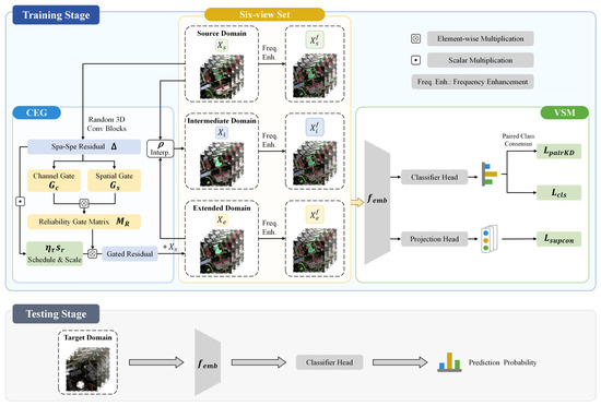
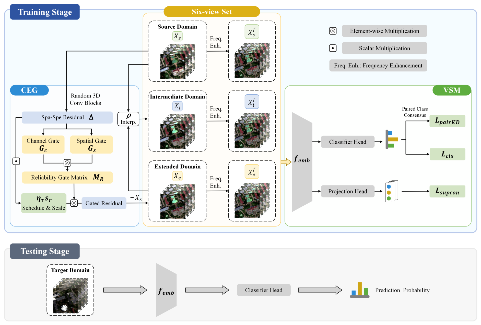
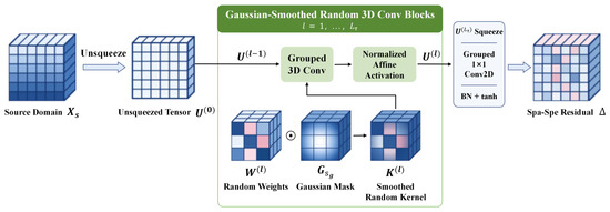
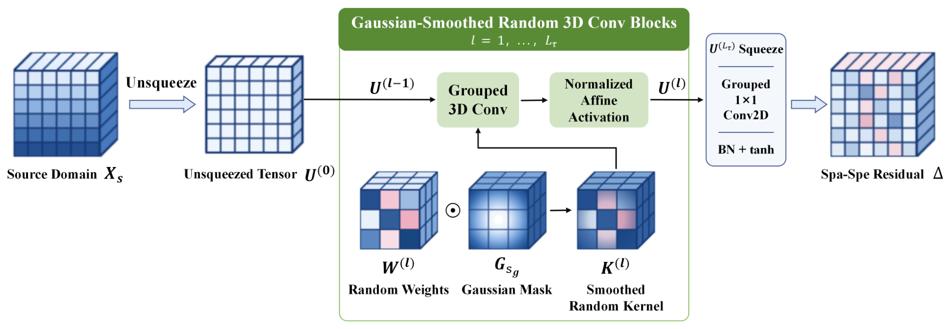
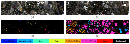
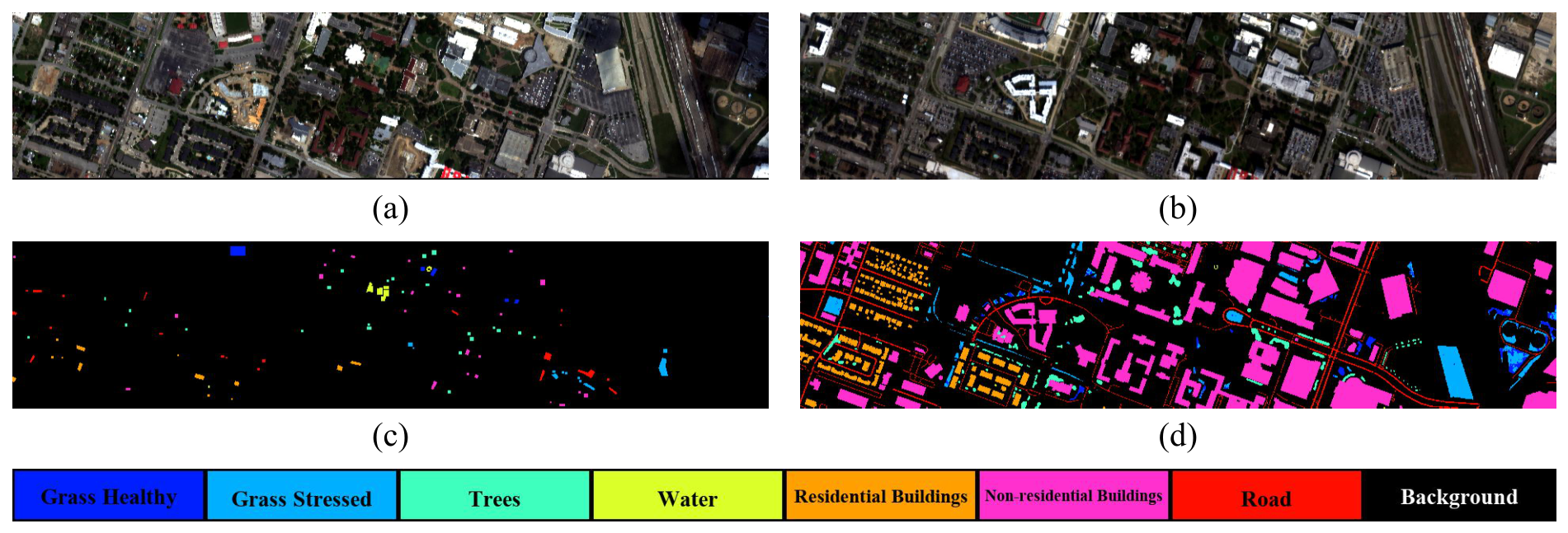
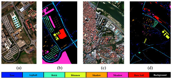
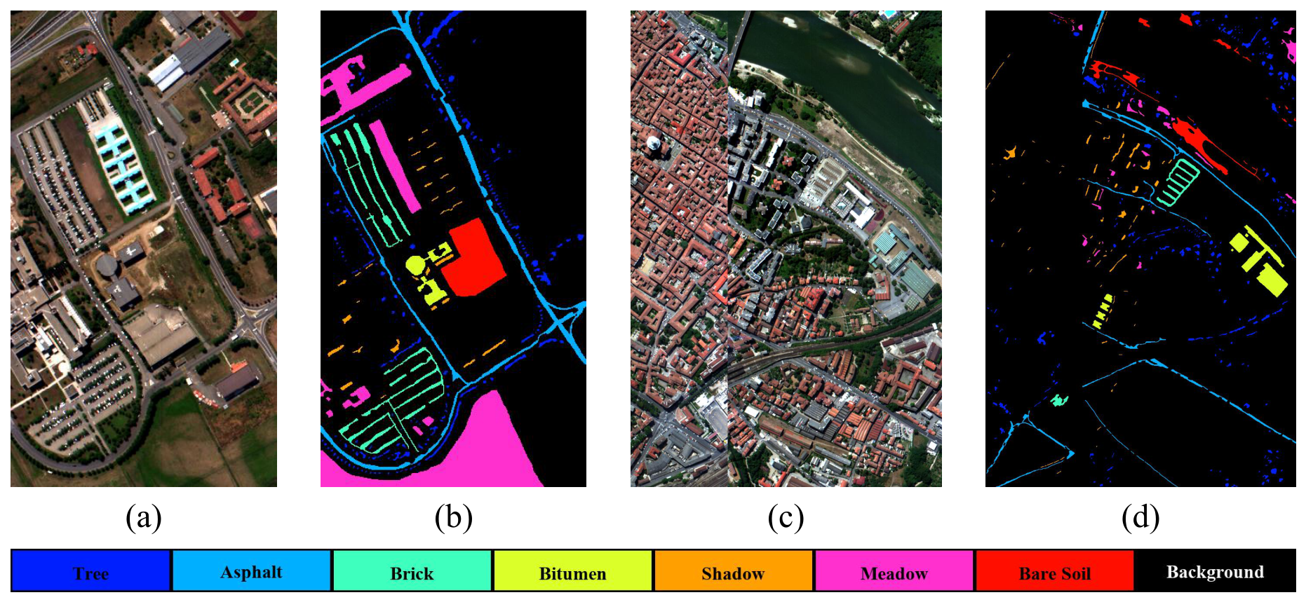
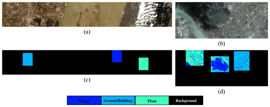
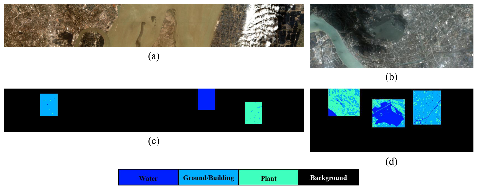
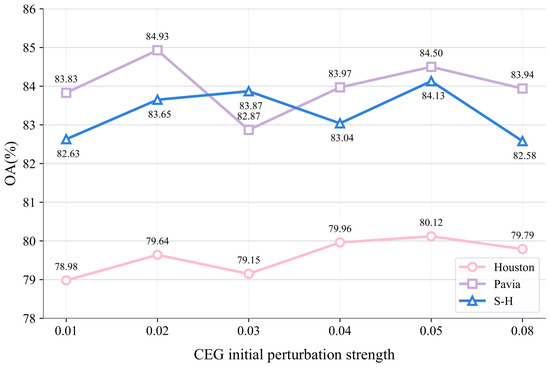
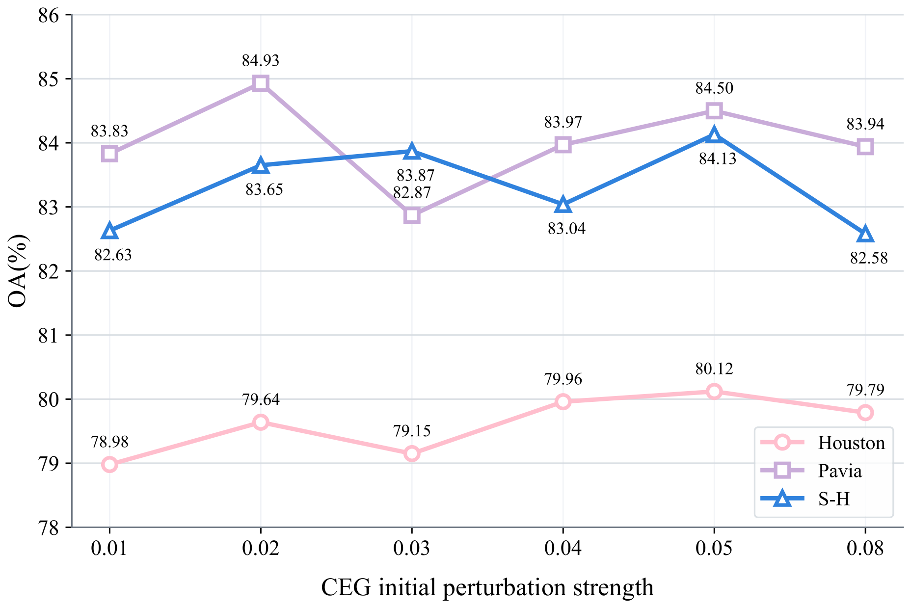
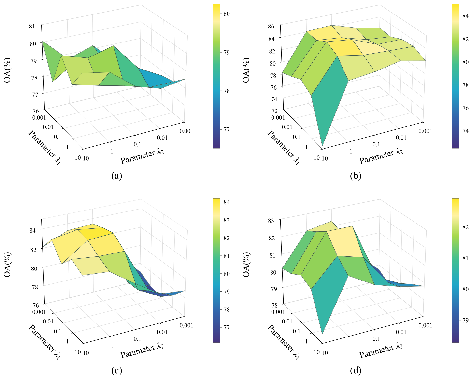
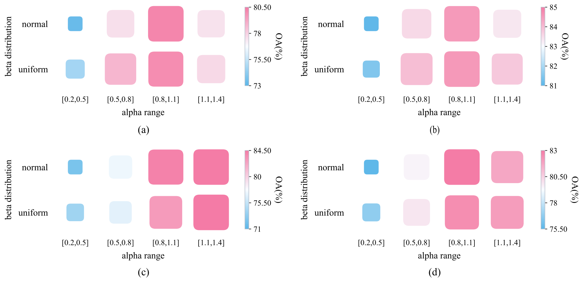
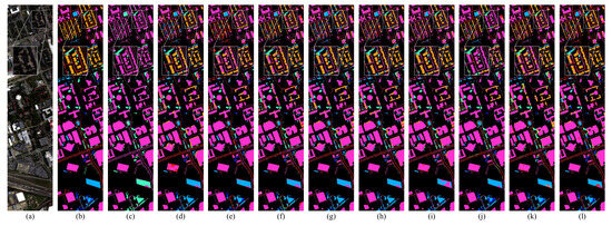
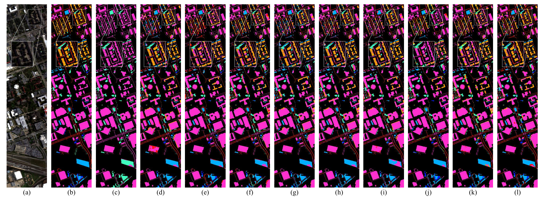
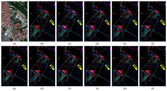
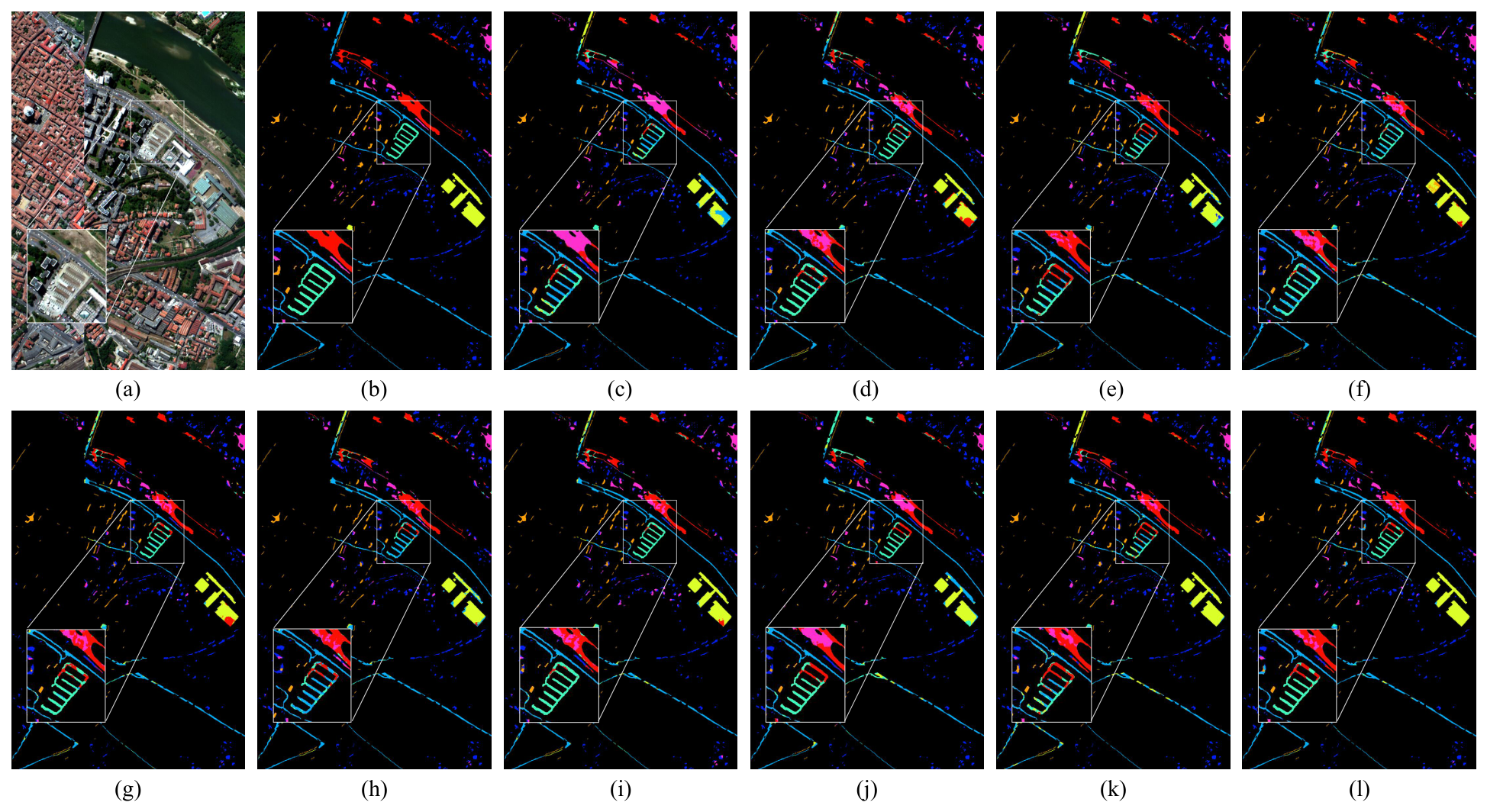
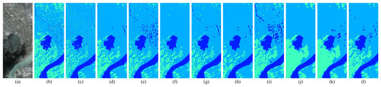
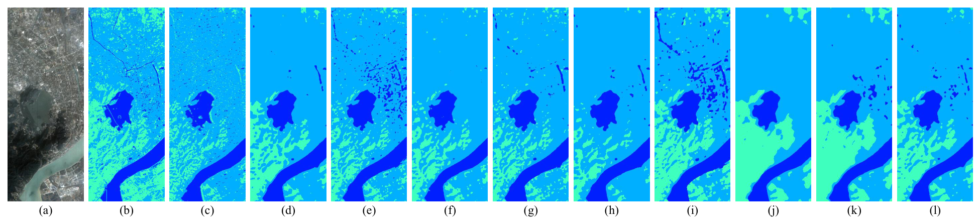
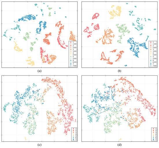
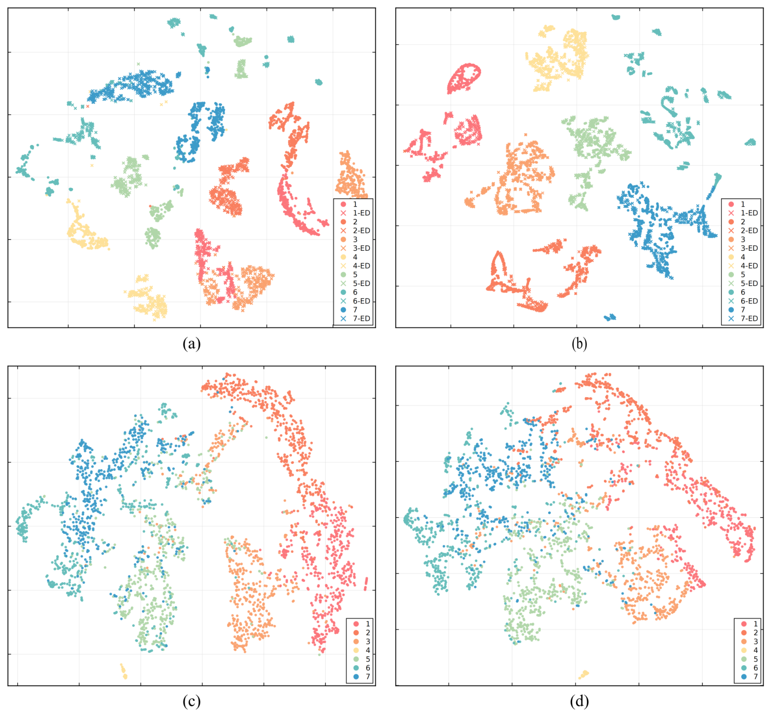
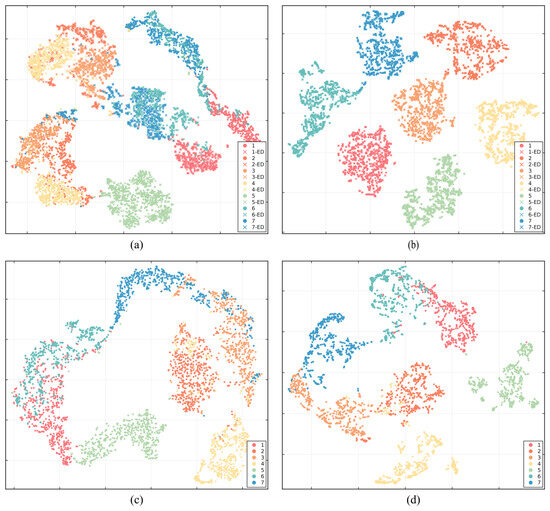
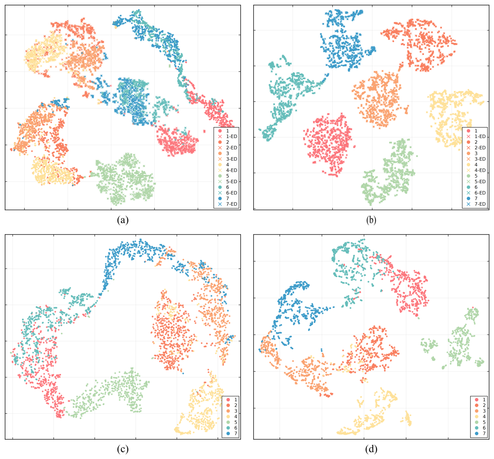
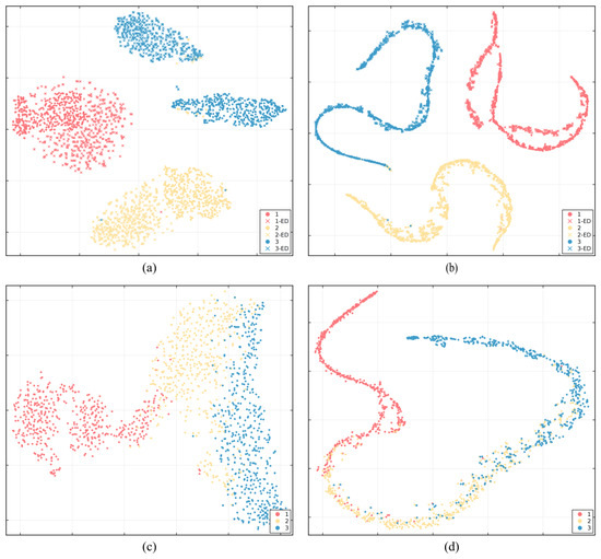
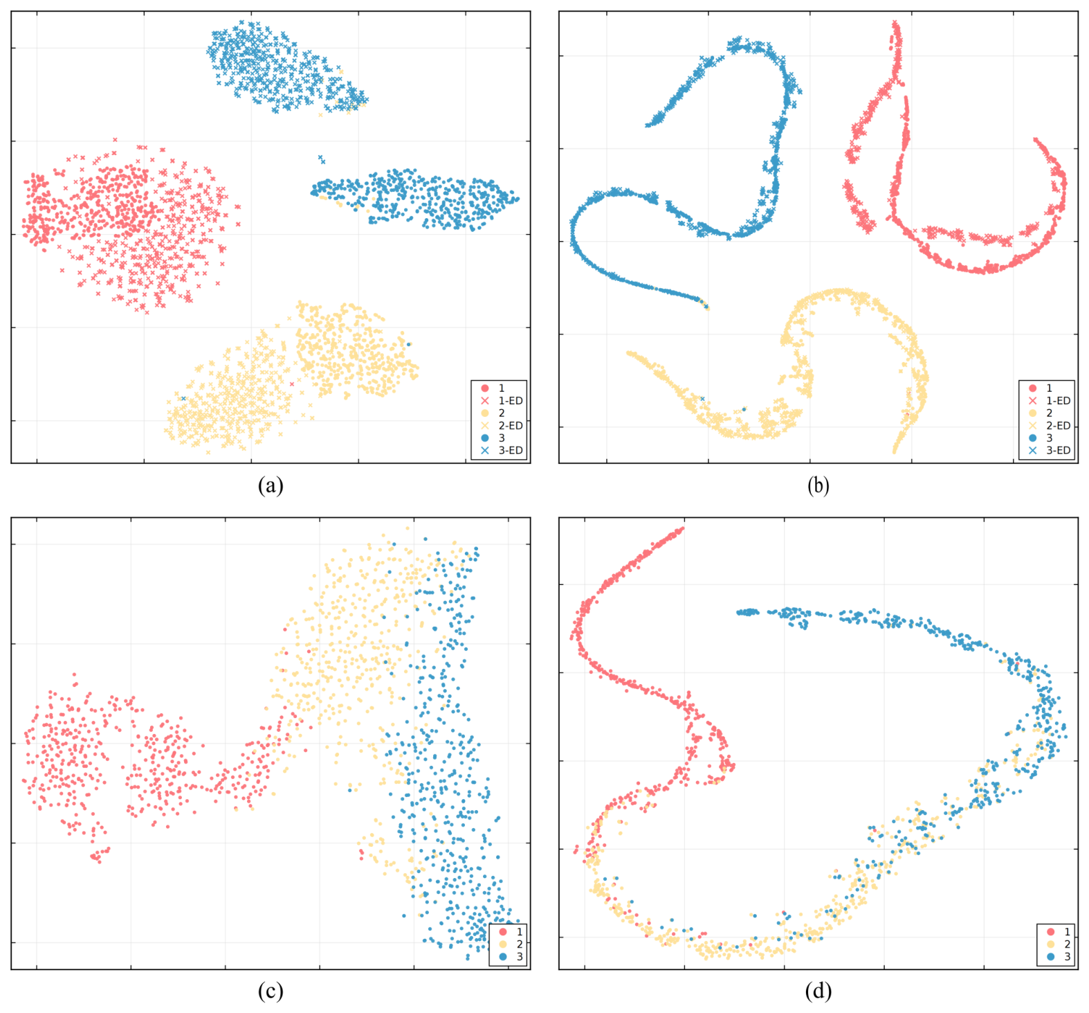
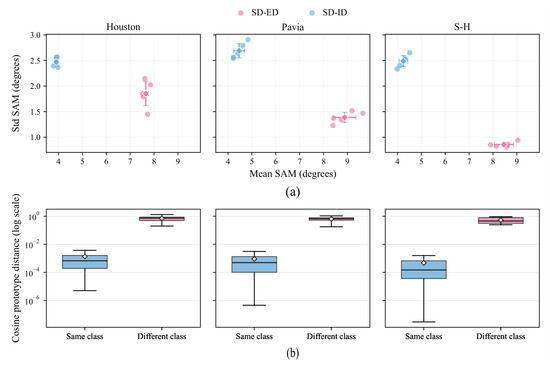
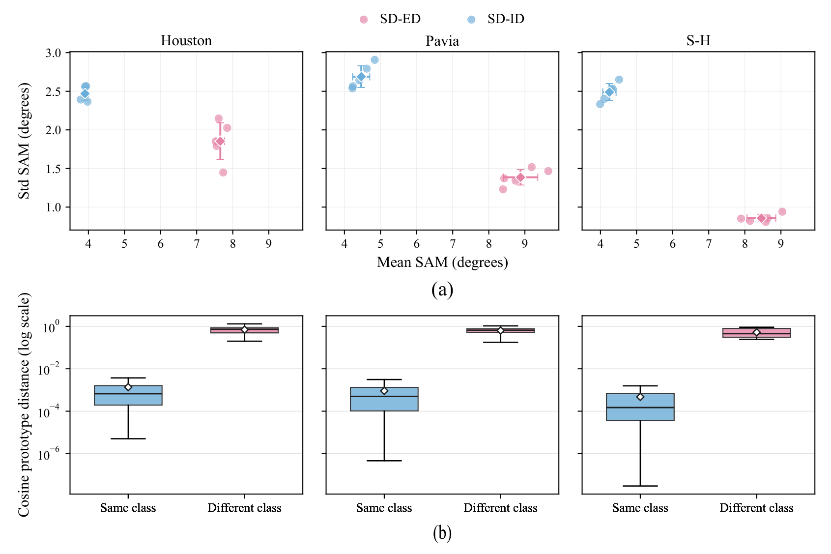

Disclaimer/Publisher’s Note: The statements, opinions and data contained in all publications are solely those of the individual author(s) and contributor(s) and not of MDPI and/or the editor(s). MDPI and/or the editor(s) disclaim responsibility for any injury to people or property resulting from any ideas, methods, instructions or products referred to in the content. |
© 2026 by the authors. Licensee MDPI, Basel, Switzerland. This article is an open access article distributed under the terms and conditions of the Creative Commons Attribution (CC BY) license.