Improving Local Climate Zone Mapping at Fine Spatial Scales Using Urban Morphology, Spectral Information, and Machine Learning

Highlights

What are the main findings?

• Sentinel-2 and PRISMA imagery combined with urban canopy parameters achieved overall accuracies of 0.79 and 0.82, respectively.
• Training-sample filtering produced limited and class-specific changes in accuracy.

What are the implications of the main findings?

• Urban canopy parameters provide valuable information for fine-scale local climate zone mapping.
• The study highlights the need to balance reductions in training-sample heterogeneity against the preservation of feature discriminative power.

Abstract

Local climate zones (LCZs) provide a robust framework for understanding Urban Heat Island dynamics and for supporting climate-sensitive urban planning. Although widely adopted since their introduction in 2012, LCZ mapping remains constrained by urban morphology description and spectral separability among built-up classes. This study aims to strengthen the methodology to produce a high-resolution LCZ map by integrating multispectral (Sentinel-2, 10 m spatial resolution) and hyperspectral data (PRISMA, 30 m spatial resolution) with a suite of urban canopy parameters that describe the morphological and surface characteristics of the urban fabric, using a machine learning classification approach at finer spatial resolutions. The proposed approach is tested in the urban area of Bologna, Italy. The digitization of representative training and validation sites—which is one of the key challenges in accurate LCZ mapping, especially for spectrally heterogeneous classes—was conducted in a GIS environment by visual interpretation of high-resolution imagery with the aid of the Technical Map of the Municipality of Bologna. With the aim of strengthening the methodology, the present work tests different outlier-removal techniques on the training data and evaluates their impact on LCZ mapping performance. Finally, the Random Forest classifier was selected, and the workflow was implemented in a Python environment using the scikit-learn library. The results show that the classification achieved overall accuracy values of 0.79 using Sentinel-2 and 0.82 using PRISMA. Overall, the results show that urban morphology parameters are among the most important features. Training-sample refinement helped interpret the effect of sample heterogeneity, but LCZ classification performance was ultimately controlled by feature discriminative power, spatial resolution, and the intrinsic separability of each class.

1. Introduction

The rapid urbanization in recent decades has led to deep soil consumption and modifications in the energy balance of cities worldwide, a phenomenon associated with global-scale climate change. One of the most relevant consequences is the Urban Heat Island (UHI) effect, where urban areas exhibit higher temperatures than surrounding non-urban areas, both at the ground level and in the canopy layer [1]. Temperature anomalies within urban areas can be attributed to altered radiative, latent and sensible heat fluxes, increased heat storage in construction materials, reduced evapotranspiration, and anthropogenic heat release [2]. Monitoring UHIs has become fundamental because higher urban temperatures directly impact energy demand, public health and air quality.

Remote sensing has become crucial in UHI research activities, especially with Thermal Infrared (TIR) observations that allow the retrieval of land surface temperature (LST), enabling spatially continuous mapping of the Surface UHI (SUHI) effect [3]. Recent reviews highlight the evolution of satellite platforms and methodologies that contribute to improved UHI assessments [4]. Among them, Mentaschi et al. [5] showed that SUHI anomalies have increased globally between 2003 and 2020 by about 1.04 K. They also found intra-urban hotspots where SUHI can exceed surrounding areas by 10–15 K. Bitelli et al. [6] developed a comprehensive methodology for retrieving surface temperatures of roofs from airborne thermal imagery and ancillary data, showing how calibrated thermal mosaics can be useful for urban climate-sensitive planning [7]. Nardino et al. [8] produced a micro-climate classification of Bologna using meteorological observations and urban morphology indicators for the development of urban sustainability.

The characterization of the spectral properties of surface materials for LCZ mapping can nowadays take advantage of a wide range of multispectral and hyperspectral satellite data. For this work, Sentinel-2 and PRISMA datasets were employed. The Sentinel-2 constellation of the European Copernicus Programme provides high-resolution multispectral imagery specifically designed to support land-monitoring applications. Each satellite in the constellation carries the multispectral instrument (MSI), capable of acquiring 13 spectral bands from the visible and near-infrared (VNIR) to the shortwave infrared (SWIR) at spatial resolutions that range from 10 to 60 m [9]. Thanks to its five-day revisit cycle at mid-latitudes, Sentinel-2 offers dense temporal coverage, enabling detailed characterization of vegetation dynamics and land-cover changes [10].

The Precursore Iperspettrale della Missione Applicativa (PRISMA) satellite of the Italian Space Agency (ASI) was launched in March 2019. The satellite carries a VNIR-SWIR imaging spectrometer with spectral resolutions better than 12 nm, a spatial resolution of 30 m, and a swath width of 30 km [11]. The hyperspectral nature of PRISMA allows for a finer discrimination of surface material differences—such as variations in vegetation pigments, building materials, soil minerals and water constituents—and has already demonstrated improved class separability compared to multispectral sensors such as Sentinel-2 [12].

The local climate zone (LCZ) classification system was introduced by Stewart and Oke in 2012 to better characterize urban areas, thus overcoming the traditional urban–rural distinction of urban landscapes [13]. It is a standardized scheme comprising 17 classes, 10 built-up classes and 7 natural land-cover types, defined by surface structure, cover, and materials. The LCZ scheme offers three key advantages: (i) a consistent set of classes that can be used to compare urban micro-climates across cities worldwide; (ii) a basis for linking morphological/land-cover characteristics to their thermal behavior; and (iii) a simple yet powerful tool dedicated to urban climate modeling.

The World Urban Database and Access Portal Tools (WUDAPT) [14] project was launched as a community-driven framework to map cities globally using the LCZ system [15]. WUDAPT has developed protocols for producing LCZ maps from freely available satellite imagery and manually digitized training areas. The WUDAPT Level 0 workflow has been shown to typically retrieve moderate overall accuracies (50–60%) [16], but shows real promise as input for urban climate models. Brousse et al. (2016) assessed the potential offered by LCZs for urban climate simulations of the city of Madrid. Their results show how LCZs improve the model performance, making them a valuable tool for climate-sensitive urban planning [17].

In recent years, LCZ mapping has advanced substantially through methodological, algorithmic, and data-related innovations, and Earth observation data have been exploited to derive LCZ maps due to their potential in continuous observations of wide areas. Early LCZ studies reported moderate accuracies due to spectral mixing and intra-class heterogeneity [18]. Subsequent research demonstrated that integrating higher-resolution optical data (e.g., Sentinel-2, Landsat, SPOT, WorldView) or combining optical and SAR information (e.g., Sentinel-1) improves the discrimination of built-up classes with similar morphology [19]. Machine learning techniques such as Random Forest (RF), Support Vector Machine (SVM), and Gradient Boosting have become widely adopted baselines for LCZ classification [20], while deep learning methods—including Convolutional Neural Networks (CNNs) and transfer learning—have further enhanced mapping performance by incorporating spatial context and textural patterns [21]. Demuzere et al. [20] were able to derive the first global LCZ map with a spatial resolution of 100 m. Simanjuntak et al. [22] compared LCZ maps derived from very-high-resolution (VHR) Pleiades and SPOT-6 imagery with those produced from Landsat data. Using Object-Based Image Analysis for VHR data and RF classification for Landsat, the authors showed that VHR imagery markedly improves LCZ delineation, with accuracies rising from 69% to 89%. Hay Chung et al. [23] suggest that RF and SVM classifiers perform best for pixel-based LCZ classification, with thermal-infrared variables being particularly influential. Recently, Vavassori et al. [24] and Vavassori et al. [25] proposed an integrated methodology combining PRISMA and Sentinel-2 imagery with GIS-derived morphological descriptors of urban areas for LCZ mapping. Their study demonstrated that hyperspectral information can substantially improve the discrimination of built-up LCZ classes when coupled with morphological descriptors. Zhao [26] produced an LCZ map for San Antonio, Texas, using a GIS-based classification, and compared LST retrieved from summer Landsat imagery across LCZ classes. Their results showed that most LCZs exhibit statistically significant temperature differences. Yang et al. [27] showed that some LCZ classes are more resilient to UHI intensity, highlighting the value of LCZ-based planning for mitigating urban thermal stress. According to Leconte et al. [28], air temperature measurements across 13 LCZs in Nancy revealed that urbanized LCZ types exhibit lower nighttime temperature amplitudes and show clear microscale hotspots and coldspots.

Recent advancements have integrated 3D urban morphology and structural parameters derived from LiDAR, photogrammetry, building databases, or high-resolution DSMs to compute detailed urban canopy parameters (UCPs) such as building height, sky view factor, tree canopy fraction, and imperviousness. These approaches significantly improve classification accuracy and class separability, especially for compact midrise and open midrise classes [29]. In the context of LCZ classification, UCPs define the geometric, thermodynamic, radiative, and surface cover properties of urban built-up and land-cover forms, proving to be crucial for urban micro-climate modeling [30]. They can be fundamental in resolving ambiguities between spectrally similar built-up classes, addressing one of the main limitations of purely spectral approaches [24]. Ching et al. [31] proposed the Digital Synthetic City, a tool that enables the derivation of UCPs that feed multi-scale atmospheric, weather and climate models. They emphasize that such synthetic modeling bridges the gap between coarse-scale LCZ maps and fine-scale morphological description. Gupta et al. [30] demonstrate that very-high-resolution satellite stereo (and UAV when available) data are suitable for deriving reliable UCPs, yielding building heights with RMSE ≈ 0.05 m and correlation coefficients > 0.8, thereby offering a viable pathway for UCP generation in data-scarce developing regions.

With the future goal of understanding the relationship between SUHIs and LCZs for the city of Bologna (Italy), the present study aims to produce an accurate LCZ map of the study area. One of the main challenges in LCZ mapping is the limited separability between built-up classes (e.g., open midrise and open low-rise), which are inherently heterogeneous and composed of varying proportions of buildings, vegetation, and impervious surfaces. This structural complexity leads to spectral mixing and reduced classification performance, particularly when using pixel-based approaches. Despite recent improvements achieved through the integration of multi-source data, the role of training data quality remains relatively underexplored. In particular, mixed and transitional pixels increase intra-class variability, limiting the ability of classifiers to capture representative class-specific feature sets. In this context, this study investigates how the refinement of training data affects the performance of the LCZ classification, while comparing the capabilities of multispectral and hyperspectral imagery within the same classification framework. Using Sentinel-2 and PRISMA imagery combined with UCPs, the impact of different filtering techniques is evaluated within a pixel-based classification framework. Rather than treating outlier removal solely as a noise reduction strategy, this work examines its role in reducing intra-class variability and its implications for representing heterogeneous urban environments.

2. Materials and Methods

2.1. Materials

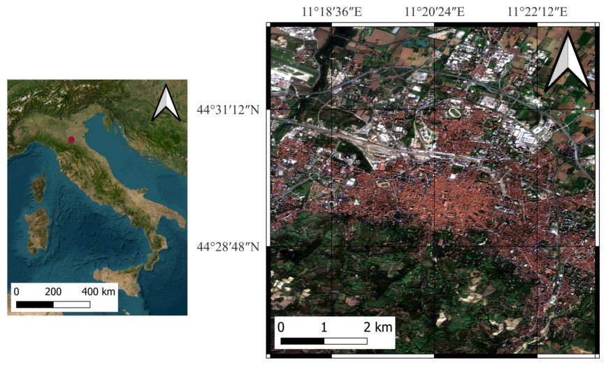
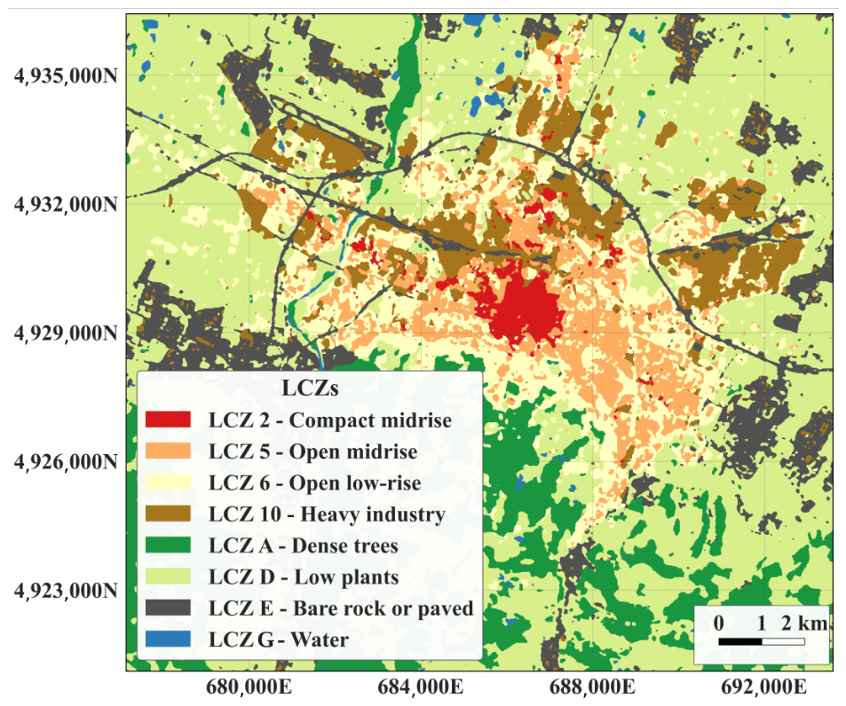
Bologna, the study area (Figure 1), is the capital of the Emilia-Romagna region in northern Italy and is located at the transition between the Po valley and the Tuscan-Emilian Apennines. The city covers almost 140 ${\mathrm{km}}^2$ and has a population of about 400,000 inhabitants [8]. The analysis was conducted over an area of approximately 200 ${\mathrm{km}}^2$ encompassing the city and its surrounding areas. Bologna exhibits a concentric urban structure, with a dense historic center characterized by medieval buildings, narrow streets, and arcades, surrounded by a garden-city belt and more recent suburban developments with wider roads and higher-density buildings. From a climatic point of view, Bologna belongs to the Cfa (temperate climate with no dry season and a hot summer) category, according to the Köppen–Geiger classification [32], with hot summers and relatively cold winters.

Two satellite images were used for the study:

• A Sentinel-2 MSI Level-2A (Surface Reflectance) image was downloaded from the Copernicus Data Space Ecosystem (Copernicus Browser). The image was collected on 26 October 2019 over tile T32TPQ. Bands B1, B9, and B10, characterized by a spatial resolution of 60 m, were excluded from the analysis. The remaining 10 spectral bands were resampled to 10 m spatial resolution, using the nearest-neighbor resampling method.
• A Level-2D PRISMA image, acquired on 24 December 2019, was downloaded from the Italian Space Agency (ASI) portal [33]. Spectral bands affected by strong atmospheric water absorption, mainly located around the main SWIR absorption regions, were removed prior to analysis to improve data quality.

The limited availability of PRISMA images fully covering the study area constrained the analysis to an early-winter PRISMA acquisition, as only two scenes suitable for this application were available between 2019 and the time of writing. However, LCZ classes are primarily defined by structural and surface characteristics. Therefore, summer-derived UCPs were used to better represent typical urban thermo-radiative conditions. The UCPs were added as additional features to both multispectral and hyperspectral data to improve the classification results. They were derived from different sources and resampled to match the spatial resolution of the Sentinel-2 and PRISMA images. Furthermore, they were normalized to a range between 0 and 1 to ensure consistency with the reflectance values. All features were stacked into a unified feature space prior to classification.

Table 1. List of the UCPs considered for the analysis.

UCP	Description	Source
Building height	Height of buildings derived from the Technical Map rasterization	Technical Map of Bologna (1:2000) [34]
Building surface fraction	Fraction of built-up area	Technical Map of Bologna (1:2000)
Tree canopy cover	Fraction of tree crown cover	Tree Cover Density 2018 (raster 10 m), Europe, 3-yearly [35]
Impervious surface fraction	Fraction of impervious surfaces	Imperviousness Density 2018 (raster 10 m), Europe, 3-yearly [36]
Land Surface Temperature	Median composite surface temperature from June to August 2019	USGS Landsat 8 Level 2, Collection 2, Tier 1 [37]
Emissivity	Median composite surface emissivity from June to August 2019	USGS Landsat 8 Level 2, Collection 2, Tier 1, ST_EMIS band [37,38]
Albedo	Surface albedo derived from a Sentinel-2 median composite from June to August 2019, using the broadband expression proposed by Bonafoni and Sekertekin [39]	Harmonized Sentinel-2 MSI: MultiSpectral Instrument, Level-2A (Surface Reflectance) [40]
Sky View Factor	Sky visibility factor derived in QGIS using the Terrain Shading plugin [41]	Technical Map of Bologna (1:2000)

lists the UCPs considered for the analysis. These variables include both morphological descriptors and thermo-radiative properties of the urban fabric.

2.2. Methods

Principal Component Analysis (PCA) was performed on the complete image feature stacks to reduce dimensionality, while preserving spectral information on both the Sentinel-2 and PRISMA acquisitions. For the Sentinel-2 case, the first 8 PCs were retrieved from a single stack containing both spectral bands and UCPs, and they explain about 99.01% of the variance of the original image. In other words, in this configuration, UCPs were included as input to the PCA transformation and were not appended as separate predictors. For the PRISMA image, the PCs were calculated in two different ways: (i) resembling Sentinel-2 configuration, both spectral bands and UCPs were stacked and given as input to generate 8 PCA bands, explaining about 98.19% of the variance of the original image (this configuration is subsequently referred to as “8 PCs”); (ii) generating the 8 PCA bands considering only the original spectral bands, which explain about 98.84% of the variance and later appending the UCPs as separate independent variables (this configuration is subsequently referred to as “8 PCs + 8 UCPs”).

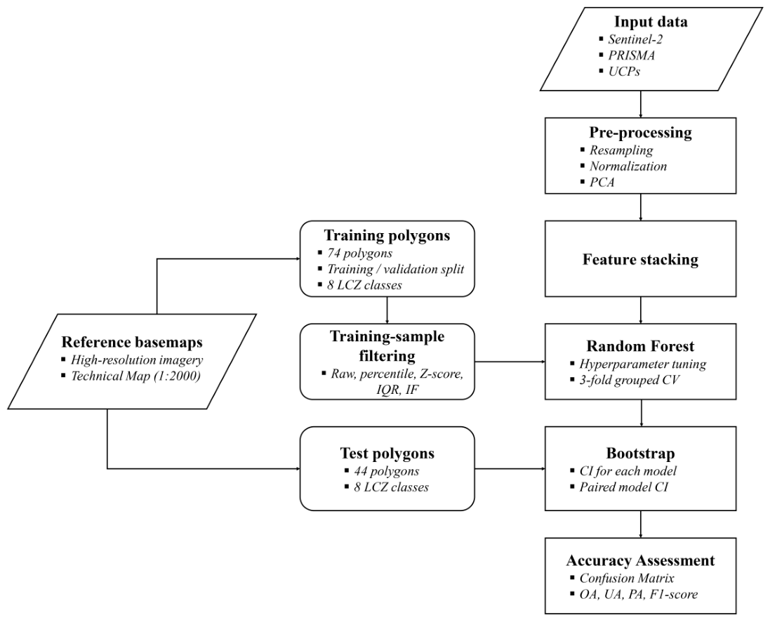
The training and the spatially independent test sites were manually digitized in a GIS environment using high-resolution imagery and the Technical Map of the Municipality of Bologna as reference basemaps. Eight representative classes from those defined in the LCZ classification system were identified within the study area: LCZ 2 (compact midrise), LCZ 5 (open midrise), LCZ 6 (open low-rise), LCZ 10 (heavy industry), LCZ A (dense trees), LCZ D (low plants), LCZ E (bare rock or paved) and LCZ G (water). Only LCZ classes that were spatially representative within the study area were considered. Several standard LCZ classes defined in the original scheme were excluded because they were either absent, extremely limited in spatial extent, or not reliably distinguishable within the available imagery and reference data. The training and test polygons were digitized following two main criteria: (i) the representativeness of each LCZ class, ensuring an adequate number of pixels to capture the intra-class spectral variability, and (ii) the spatial extent of the polygons, in accordance with WUDAPT guidelines, which recommend training areas of at least 250 m × 250 m to properly represent the spatial structure of each LCZ type. A total of 74 and 44 polygons were selected for training and test, respectively. These polygons were used to extract the pixels required for classifier training, internal validation, and independent testing. The original training polygons were further split into training (80%) and validation (20%) subsets at the polygon level, using a stratified random sampling approach to preserve the LCZ class proportions and minimize the effect of spatial autocorrelation. No test polygon overlapped or shared a boundary with any training polygon, confirming the spatial separation of the two sets.

Because Sentinel-2 and PRISMA have different spatial resolutions, the same reference polygons produced different numbers of sampled pixels for the two sensors. The independent test set contained 35,859 pixels for Sentinel-2 and 4125 pixels for PRISMA. The class-wise distribution of polygons and sampled pixels is reported in

Table 2. Number of reference polygons and sampled pixels per LCZ class for Sentinel-2. Pixel counts refer to the full unfiltered sample set extracted from the training and independent test polygons.

Class	Training Polygons	Training Pixels	Test Polygons	Test Pixels
Bare rock or paved	12	4141	6	2857
Compact midrise	6	5361	3	3833
Dense trees	9	9464	3	5235
Heavy industry	4	8146	3	5455
Low plants	7	9833	4	5107
Open low-rise	17	11,325	13	6068
Open midrise	11	10,742	6	5735
Water	8	2713	6	1569

and

Table 3. Number of reference polygons and sampled pixels per LCZ class for PRISMA. Pixel counts refer to the full unfiltered sample set extracted from the training and independent test polygons.

Class	Training Polygons	Training Pixels	Test Polygons	Test Pixels
Bare rock or paved	12	584	6	391
Compact midrise	6	595	3	425
Dense trees	9	1049	3	634
Heavy industry	4	911	3	587
Low plants	7	1108	4	566
Open low-rise	17	1263	13	674
Open midrise	11	1193	6	640
Water	8	346	6	208

. Pixel counts represent the nominal sample size, whereas the effective independent sampling units are the reference polygons.

To quantify the effect of intra-class spectral heterogeneity, particularly within built-up LCZ classes, outlier removal techniques were applied to the training sample (Section 2.3). Indeed, the manual delineation of training and test polygons through photo-interpretation may have introduced spectrally inconsistent pixels, while the resampling of several of the UCPs may have altered the representation of fine-scale urban morphology.

A machine learning model, specifically Random Forest (RF), was employed for the classification, and the analyses were carried out in a Python environment using the scikit-learn library. RF was selected because it has demonstrated robust performance in LCZ classification tasks, can effectively model non-linear relationships, and performs well with limited training datasets compared to more data-demanding deep learning approaches [20]. To optimize the RF classifier and ensure robust performance across all LCZ classes, hyperparameter optimization was performed using the function GridSearchCV provided in the scikit-learn package, version 1.7.2 with 3-fold polygon-level grouped cross-validation, ensuring that pixels extracted from the same polygon were never assigned to different folds during model selection. The optimal hyperparameter set was selected by maximizing the macro F1-score (i.e., the arithmetic mean of the F1-scores across classes), in order to balance performance across LCZ classes, particularly those with heterogeneous spectral characteristics. The investigated GridSearchCV search grid consisted of the following:

• Number of trees: 100, 200, 300;
• Criterion: Gini or entropy;
• Maximum tree depth: 10, 20, 30, or no limit;
• Minimum samples per split: 2, 5, or 10;
• Minimum samples per leaf: 1, 2, 4, 8, or 10;
• Feature sampling: square-root or log2;
• Bootstrap: true or false;
• Class weighting: none, balanced, or balanced-subsample.

After hyperparameter selection, the final classifier was trained on the selected training samples.

The classification accuracy was evaluated on the raw thematic map by constructing the confusion matrices and calculating the associated metrics, including overall accuracy (OA), precision, recall, and F1-score. In this study, precision and recall are hereafter referred to as user accuracy (UA) and producer accuracy (PA), respectively. The assessment was conducted in two stages: (i) evaluation of the validation pixels to assess the capability of the model to generalize to unseen data and (ii) evaluation of the spatially independent testing dataset to determine the accuracy of the final LCZ maps. The assessment based on the full, unfiltered independent test set was considered the main accuracy estimate for the LCZ maps because it included mixed, transitional, and spectrally heterogeneous pixels that were also present in the final classified map.

To quantify the uncertainty of the accuracy estimates, 95% confidence intervals (CIs) were computed using a polygon-level bootstrap procedure. For each bootstrap iteration, the independent test polygons were sampled with replacement, and all pixels belonging to the selected polygons were included in the resampled evaluation set. The procedure was repeated 1000 times. For each bootstrap sample, OA, macro F1-score, and weighted F1-score (i.e., average F1 weighted by the number of test pixels) were calculated. Resampling was not stratified by class, so classes represented by a small number of test polygons could be absent from individual replicates. All bootstrap replicates were retained. For each replicate, OA was calculated as the proportion of correctly classified pixels. The macro F1-score was calculated over the union of classes present in the reference or predicted labels. Consequently, a class absent from both the reference and predicted labels was excluded from the average, whereas a class absent from the reference labels but still predicted by the classifier was included, with an F1-score of zero.

Following validation, the optimized classifiers were applied to the entire study area to generate the final LCZ thematic maps.

Figure 2 summarizes the adopted methodology.

2.3. Outlier Removal Techniques

To mitigate intra-class heterogeneity and reduce the impact of anomalous samples, particularly relevant for built-up LCZ classes characterized by mixed materials and boundary effects, different outlier detection techniques were applied to the feature space prior to model training. All methods were applied independently to each LCZ class, ensuring that class-specific statistical properties were preserved.

The following approaches were considered, representing different assumptions about data distribution and anomaly structure:

• Percentile Trimming
  This is a non-parametric method that removes extreme observations based on empirical quantiles. For each class c and feature j, the 2nd and 98th percentiles were calculated, and pixels falling outside the thresholds defined in Equation (1), in at least one feature, were removed.

  $$\begin{array}{c}\hfill x_{ij}^{\left(c\right)}<Q_{0.02}^{(c,j)}\mathrm{or}{x}_{ij}^{\left(c\right)}>Q_{0.98}^{(c,j)}\end{array}$$

  (1)
  This approach does not assume any underlying distribution and is robust to skewed data.
• Z-Score Filtering
  This is a parametric method based on standardization. For each class c and feature j, the standardized score is computed as

  $$\begin{array}{c}\hfill z_{ij}^{\left(c\right)}={\displaystyle \frac{x_{ij}^{\left(c\right)}-{\mu }_j^{\left(c\right)}}{{\sigma }_j^{\left(c\right)}}}\end{array}$$

  (2)

  where $x_{ij}$ is the ith pixel, $\mu$ and $\sigma$ are the mean and the standard deviation of the jth feature. Pixels exceeding the threshold defined in Equation (3), in at least one feature, were considered outliers and removed from the data.

  $$\begin{array}{c}\hfill \left|z_{ij}^{\left(c\right)}\right|>2\end{array}$$

  (3)
  It is acknowledged that, under strict normality, this threshold removes approximately 5% of valid samples per feature by construction; however, given the non-Gaussian nature of urban spectral distributions, the removed observations may include mixed or transitional pixels as well as valid extremes of heterogeneous LCZ classes.
• Interquartile Range (IQR)
  This is a robust statistical approach based on quartiles. For each class c and feature j, pixels falling below or above the limits defined in Equation (4), in at least one feature, were excluded.

  $$\begin{array}{c}\hfill {\mathrm{IQR}}^{(c,j)}=Q_{0.75}^{(c,j)}-Q_{0.25}^{(c,j)}\\ \hfill x_{ij}^{\left(c\right)}<Q_{0.25}^{(c,j)}-1.5·{\mathrm{IQR}}^{(c,j)}\\ \hfill x_{ij}^{\left(c\right)}>Q_{0.75}^{(c,j)}+1.5·{\mathrm{IQR}}^{(c,j)}\end{array}$$

  (4)
  This method is robust to non-Gaussian distributions and is widely used in exploratory data analysis.
• Isolation Forest (IF)
  Isolation Forest is a machine learning-based anomaly detection method that identifies outliers by recursively partitioning the feature space [42]. Samples that require fewer splits to be isolated are more likely to be anomalous. The algorithm was applied independently to each class, and samples flagged as anomalies were removed. A total of 300 trees were chosen, with the contamination parameter set to “auto”, so anomaly labels were assigned using the automatic decision threshold implemented in scikit-learn.

These methods provide a spectrum of filtering strategies, from simple distribution-based trimming to model-based anomaly detection, enabling a systematic evaluation of their impact on LCZ classification performance. The parameters governing each outlier removal method were selected to ensure comparability across techniques while maintaining a reasonable balance between removal aggressiveness and sample retention.

3. Results

Figure 3 reports the class-wise F1-score comparison among the tested feature configurations for Sentinel-2 and PRISMA, evaluated on the full unfiltered independent test set. Based on this comparison, the Sentinel-2 (10 spectral bands + 8 UCPs) and PRISMA (8 spectral PCs + 8 UCPs) configurations were selected for further analyses because they achieved the highest macro F1-score (0.81 and 0.83, respectively). These configurations were used to assess the effects of training-sample filtering, spatial resolution, and feature importance.

3.1. Baseline Results

The baseline classification results, obtained using raw unfiltered training samples and evaluated on the unfiltered independent test set, are reported in

Table 4. Observed class-wise accuracy metrics for the Sentinel-2 baseline configuration (10 spectral bands + 8 UCPs), evaluated on the full, unfiltered independent test set. The RF classifier was trained using the unfiltered training pixels.

Class	User Accuracy	Producer Accuracy	F1-Score
Bare rock or paved	0.95	0.92	0.94
Compact midrise	0.76	0.84	0.80
Dense trees	0.96	0.78	0.86
Heavy industry	0.87	0.83	0.85
Low plants	0.85	0.99	0.92
Open low-rise	0.63	0.65	0.64
Open midrise	0.61	0.61	0.61
Water	0.93	0.84	0.88

and

Table 5. Observed class-wise accuracy metrics for the PRISMA baseline configuration (eight PCs + eight UCPs), evaluated on the full, unfiltered independent test set. The RF classifier was trained using the unfiltered training pixels.

Class	User Accuracy	Producer Accuracy	F1-Score
Bare rock or paved	0.83	0.93	0.88
Compact midrise	0.83	0.88	0.85
Dense trees	0.97	0.81	0.88
Heavy industry	0.86	0.91	0.88
Low plants	0.87	0.96	0.91
Open low-rise	0.71	0.68	0.69
Open midrise	0.67	0.65	0.66
Water	0.92	0.87	0.89

. The Sentinel-2 image achieved an OA of 0.79, a macro F1-score of 0.81, and a weighted F1-score of 0.79. The PRISMA image achieved an OA of 0.82, a macro F1-score of 0.83, and a weighted F1-score of 0.82.

The observed class-wise accuracy metrics show that spectrally homogeneous classes, including dense trees (LCZ A), low plants (LCZ D), bare rock or paved (LCZ E), and water (LCZ G), achieved high performance, with F1-scores generally exceeding 0.85. In contrast, built-up classes exhibit lower accuracy. In particular, open midrise (LCZ 5) and open low-rise (LCZ 6) show the lowest performance, with F1-scores below 0.70 in both Sentinel-2 and PRISMA scenes. The confusion matrices shown in Figure 4 highlight misclassification patterns primarily between these two classes.

3.2. Training Sample Filtering

The application of outlier removal techniques resulted in substantial differences in the proportion of training samples retained, as shown in

Table 6. Percentage of training pixels removed for Sentinel-2 (10 spectral bands + 8 UCPs) for each method.

Class	Percentile	Z-Score	IQR	IF
Bare rock or paved	23.6%	30.6%	39.8%	10.5%
Compact midrise	22.6%	33.0%	35.9%	12.6%
Dense trees	22.2%	23.3%	19.6%	10.4%
Heavy industry	22.5%	35.0%	25.6%	12.2%
Low plants	26.4%	22.9%	14.8%	14.3%
Open low-rise	24.4%	32.6%	27.6%	14.2%
Open midrise	25.8%	33.3%	16.2%	11.4%
Water	29.8%	23.6%	32.7%	10.8%

and

Table 7. Percentage of training pixels removed for PRISMA (eight PCs + eight UCPs) for each method.

Class	Percentile	Z-Score	IQR	IF
Bare rock or paved	35.7%	46.5%	45.3%	4.5%
Compact midrise	35.7%	46.2%	40.7%	5.5%
Dense trees	30.8%	34.4%	30.4%	8.8%
Heavy industry	33.2%	44.3%	41.2%	7.8%
Low plants	34.2%	30.8%	15.9%	7.0%
Open low-rise	33.1%	38.9%	38.1%	9.4%
Open midrise	34.1%	43.8%	45.2%	7.2%
Water	27.3%	32.9%	49.0%	10.1%

. For Sentinel-2, removal rates range globally between approximately 10% and 40%, depending on the filtering strategy. In contrast, PRISMA exhibits systematically higher removal rates, reaching values up to 50% for certain classes. Furthermore, among the tested approaches, Z-score and IQR filtering produce the highest removal rates, while percentile trimming shows more moderate reductions. Isolation Forest removed a varying proportion of pixels depending on the image and class, generally ranging between approximately 10–15% for Sentinel-2 and 4–11% for PRISMA.

Table 8. Classification performance for the Sentinel-2 (10 spectral bands + 8 UCPs) image, using different training-sample filtering strategies. Metrics were computed on the full unfiltered independent test set. Values in brackets indicate 95% CIs obtained by polygon-level bootstrap resampling.

Training Samples	OA	Macro F1-Score	Weighted F1-Score
Raw	0.79 [0.72–0.89]	0.81 [0.64–0.86]	0.79 [0.71–0.89]
Percentile	0.80 [0.74–0.88]	0.82 [0.66–0.85]	0.80 [0.75–0.88]
Z-score	0.81 [0.76–0.87]	0.83 [0.66–0.86]	0.81 [0.76–0.87]
IQR	0.79 [0.72–0.86]	0.79 [0.61–0.83]	0.79 [0.72–0.86]
Isolation Forest	0.80 [0.74–0.88]	0.82 [0.65–0.86]	0.81 [0.75–0.88]

and

Table 9. Classification performance for the PRISMA (eight PCs + eight UCPs) image, using different training-sample filtering strategies. Metrics were computed on the full unfiltered independent test set. Values in brackets indicate 95% CIs obtained by polygon-level bootstrap resampling.

Training Samples	OA	Macro F1-Score	Weighted F1-Score
Raw	0.82 [0.75–0.91]	0.83 [0.66–0.87]	0.82 [0.74–0.91]
Percentile	0.82 [0.76–0.90]	0.83 [0.68–0.87]	0.82 [0.77–0.91]
Z-score	0.81 [0.73–0.89]	0.82 [0.65–0.86]	0.80 [0.73–0.90]
IQR	0.80 [0.73–0.86]	0.79 [0.62–0.85]	0.80 [0.73–0.87]
Isolation Forest	0.83 [0.77–0.90]	0.84 [0.67–0.87]	0.83 [0.77–0.91]

summarize the classification performance obtained with the different training-sample filtering strategies and evaluated on the full unfiltered independent test set. The 95% confidence intervals (reported in brackets) were estimated through polygon-level bootstrap resampling. For Sentinel-2 (10 spectral bands + 8 UCPs), OA ranged from 0.79 to 0.81, with the highest value obtained using Z-score filtering. Percentile and Isolation Forest produced values close to the raw baseline, while IQR showed negligible improvement. For PRISMA (eight PCs + eight UCPs), OA ranged from 0.80 to 0.83, with the highest value obtained using Isolation Forest. Percentile filtering remained close to the raw baseline, whereas Z-score and IQR produced lower values.

Figure 5 presents the point-estimated class-wise F1-scores obtained by the models shown in Table 8 and Table 9, highlighting a class-dependent response.

To assess the robustness of the observed differences among training-sample filtering strategies, each resulting model was compared with the corresponding raw baseline on the unfiltered test set (Figure 6 and Figure 7). Differences in OA, macro F1-score, and weighted F1-score were expressed relative to the raw baseline and their uncertainty was quantified through paired polygon-level bootstrap resampling.

For Sentinel-2, Z-score filtering produced the largest positive point-estimate differences relative to the raw baseline, whereas Isolation Forest and percentile produced smaller positive differences and IQR remained close to or below the baseline. For PRISMA, Isolation Forest produced the largest positive point estimates, percentile remained nearly unchanged, and Z-score and IQR produced negative differences.

3.3. The Effect of Spatial Resolution

To further investigate the effect of spatial resolution, an additional experiment was conducted by resampling the Sentinel-2 image to a spatial resolution of 30 m using bilinear interpolation. The resampled Sentinel-2 configuration reached an OA of 0.76 [0.67–0.83], a macro-F1 of 0.76 [0.59–0.82], and a weighted F1 of 0.76 [0.67–0.84].

Table 10. Observed class-wise accuracy metrics for the resampled Sentinel-2 (10 spectral bands + 8 UCPs) image evaluated using the unfiltered independent test set. The RF classifier was trained using the unfiltered training pixels.

Class	User Accuracy	Producer Accuracy	F1-Score
Bare rock or paved	0.65	0.88	0.75
Compact midrise	0.81	0.83	0.82
Dense trees	0.94	0.77	0.84
Heavy industry	0.88	0.86	0.87
Low plants	0.88	0.89	0.89
Open low-rise	0.66	0.65	0.65
Open midrise	0.60	0.63	0.62
Water	0.76	0.55	0.63

shows the point estimate accuracy metrics of the resampled Sentinel-2 image.

Compared with the original Sentinel-2 configuration, the strongest reductions in F1-score were observed for bare rock or paved and water, while dense trees and low plants showed smaller decreases (Figure 8). In contrast, the built-up classes remained broadly comparable between the two spatial resolutions, with minor differences for compact midrise, heavy industry, open low-rise, and open midrise. These results suggest that the loss of fine-scale spatial detail affects LCZ separability, although the magnitude of the effect varies across classes.

3.4. Feature Importance and Final LCZ Map

Figure 9 shows the top 10 features ranked by permutation importance for the selected Sentinel-2 and PRISMA configurations. Across both datasets, several UCPs ranked among the most influential predictors, supporting the complementary relevance of urban morphology and thermo-radiative surface descriptors for LCZ discrimination.

Figure 10 shows the LCZ map derived from the Sentinel-2 image (10 spectral bands + 8 UCPs), post-processed using a 7 × 7 majority moving window to reduce pixel-level noise and improve the spatial consistency of the classes.

4. Discussion

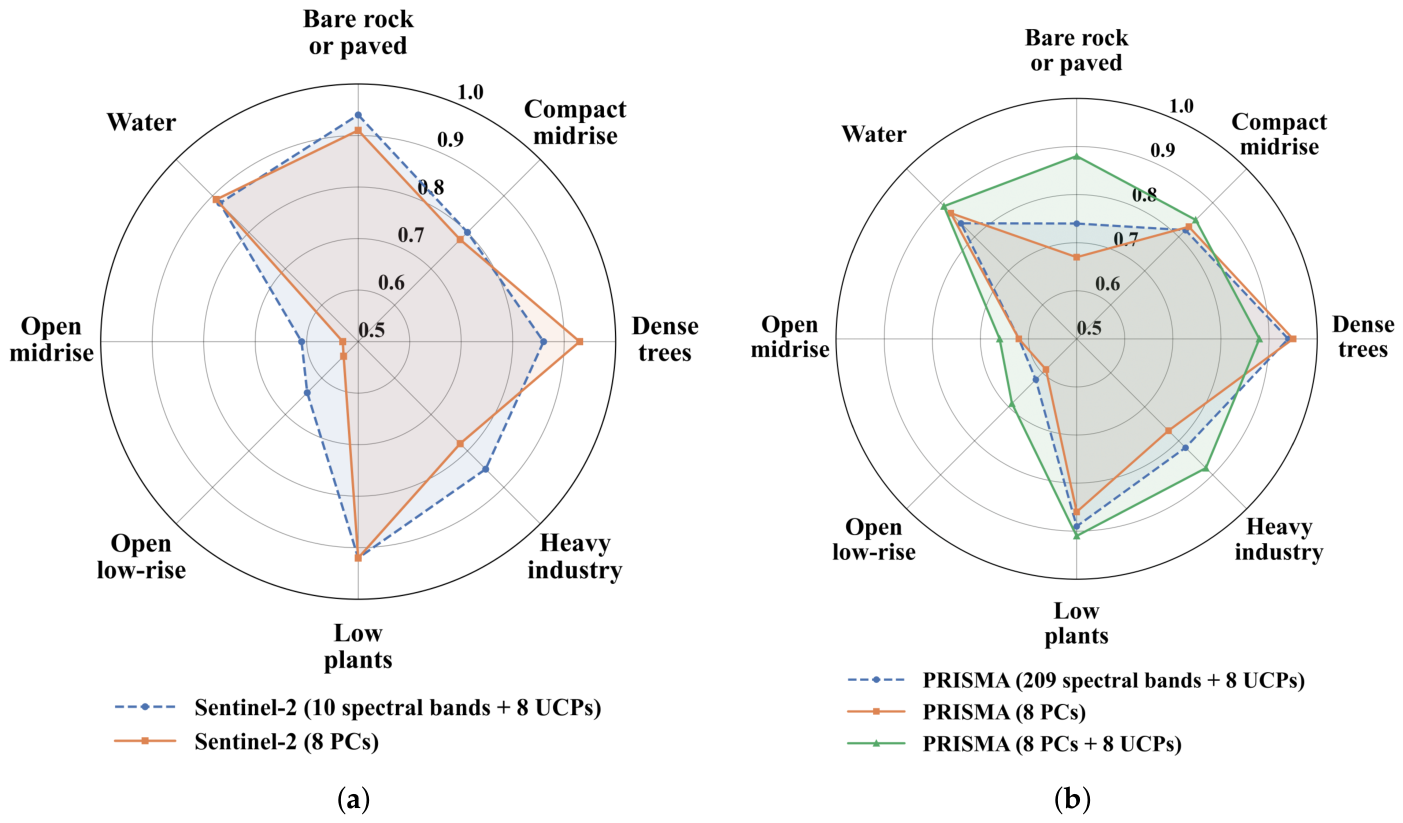
The baseline results confirm that LCZ classification performance is strongly affected by intra-class heterogeneity and by the limited separability of morphologically similar built-up classes. Figure 3 reveals the key role played by the composition of the feature space. For Sentinel-2, the feature space composed of 10 spectral bands and the 8 UCPs provided a suitable reference configuration, whereas considering its first 8 PCs did not clearly improve the class-wise performance. For PRISMA, the feature space composed of eight PCs + eight UCPs provided the most balanced performance across classes (in terms of point estimates). Dimensionality reduction therefore appears useful for compressing hyperspectral information and reducing redundancy, while the UCPs retain supplementary information on urban morphology and surface properties [24].

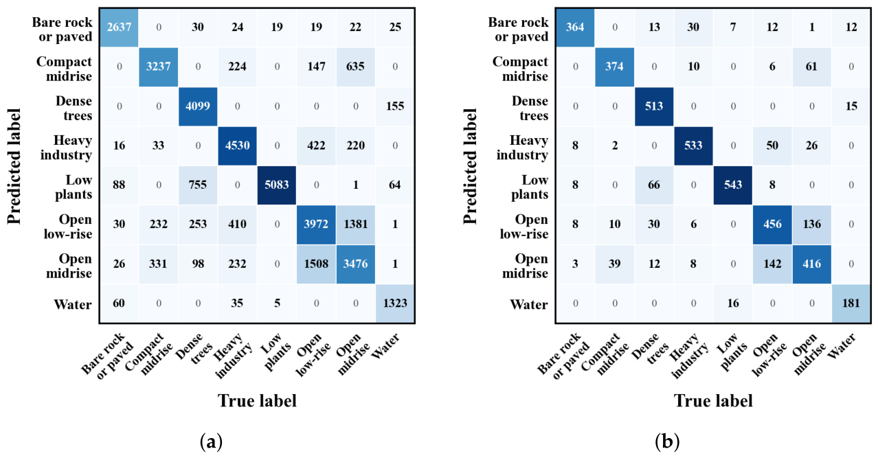
In both Sentinel-2 and PRISMA configurations (Table 4 and Table 5), homogeneous classes, such as dense trees, low plants, bare rock or paved, and water, achieved relatively high F1-scores (>0.80). In contrast, open low-rise and open midrise were consistently the most challenging LCZ types, with the lowest F1-scores among the evaluated classes (<0.70). The confusion matrices (Figure 4) show that most of the errors involving these classes occur between open low-rise, open midrise, and, to a lesser extent, heavy industry. This pattern reflects the structural and spectral complexity of these LCZ types, which often contain different proportions of buildings, vegetation, and impervious surfaces. Similar confusion among built-up LCZ classes has also been reported in previous studies, where structural similarity and mixed urban surfaces reduce class separability [29,43,44].

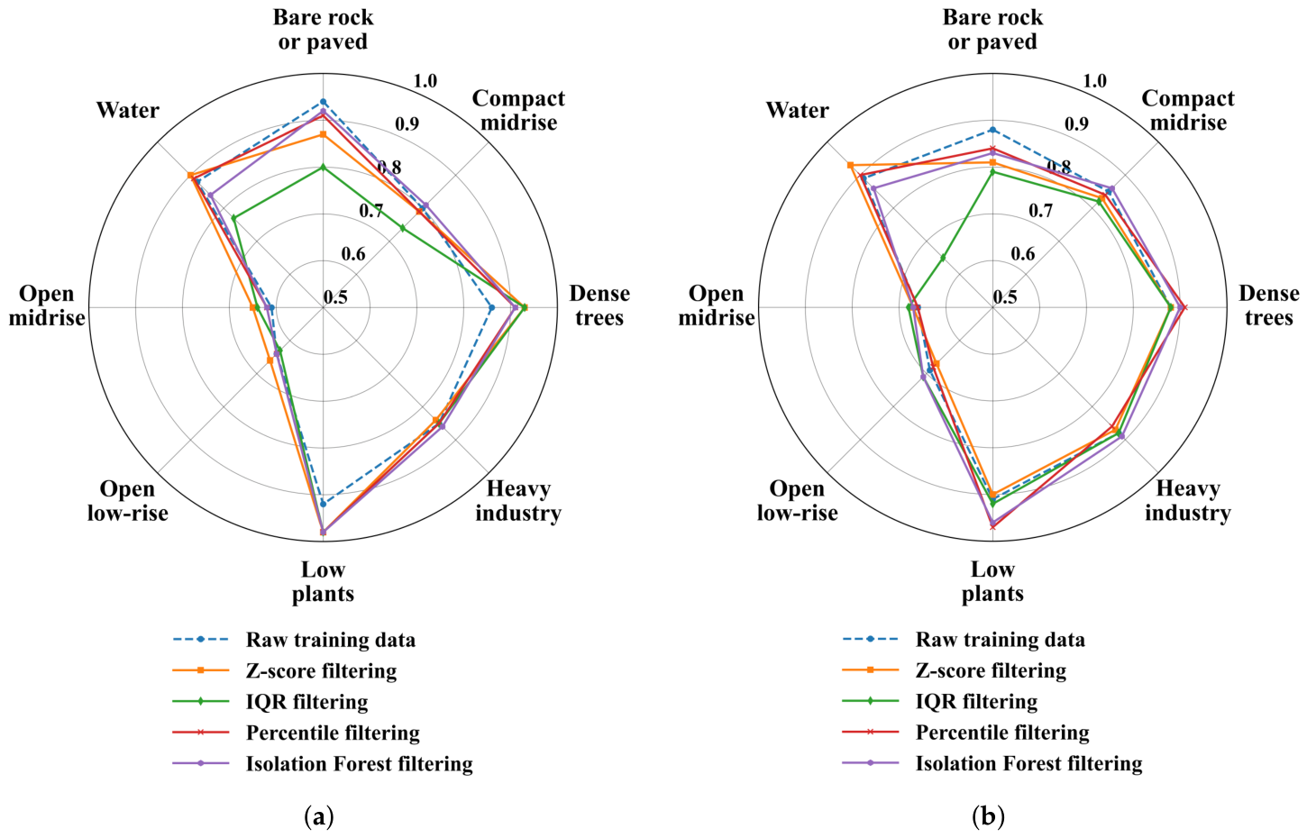
Filtering produced substantial changes in the composition of the training data, but these changes resulted in limited variations in classification performance. Figure 5 shows that the response was class-dependent: changes were generally small for the heterogeneous built-up classes, whereas bare rock or paved, low plants, and water showed more pronounced variations.

The removal rates also differed clearly between Sentinel-2 and PRISMA (Table 6 and Table 7). For Sentinel-2, threshold-based methods generally removed between about 20% and 40% of the training pixels, while Isolation Forest removed a smaller fraction, approximately 10–15%. For PRISMA, percentile, Z-score, and IQR filtering were more aggressive, often removing more than 30% of the samples and reaching nearly 50% for some classes. This behavior may suggest that the PRISMA feature space produced broader within-class distributions; however, the different nominal sample sizes associated with the two sensors are also relevant. Although Sentinel-2 and PRISMA were evaluated using the same independent test polygons, the number of pixels was much larger for Sentinel-2 than for PRISMA because of their different spatial resolutions. Therefore, when a filtering method removes a high percentage of PRISMA pixels, the remaining training set becomes much smaller in absolute terms than the corresponding Sentinel-2 training set. This can reduce the ability of the classifier to learn the full variability of each LCZ class, especially for classes already represented by a limited number of polygons.

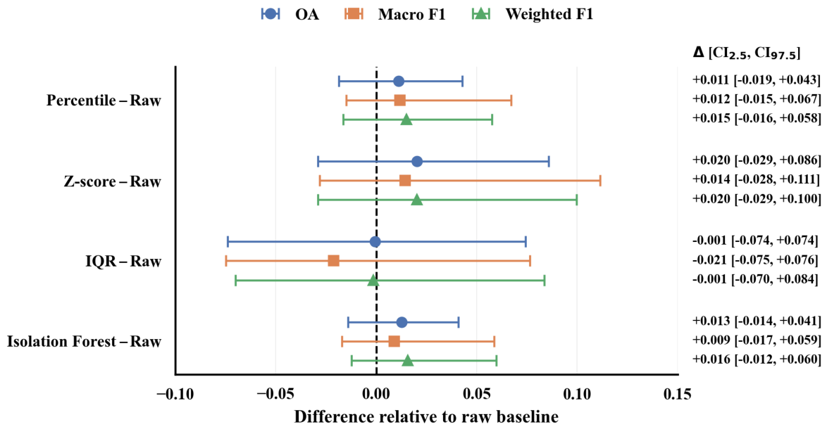
Table 8 and Table 9 show that for Sentinel-2, Z-score filtering produced the highest point estimates, with OA increasing from 0.79 to 0.81 and both Macro and weighted F1-scores also increasing slightly. Percentile and Isolation Forest produced values close to the raw baseline, while IQR did not improve the results. This suggests that, in the Sentinel-2 feature space, moderate filtering may remove part of the ambiguous or inconsistent training pixels without excessively reducing class representativeness. 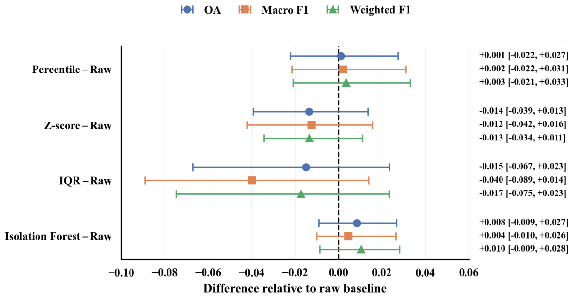However, the magnitude of the improvement remained small, and the paired bootstrap CIs for the differences relative to the raw baseline crossed zero, indicating that the effect was not conclusive (Figure 6). For PRISMA, the pattern is different. Isolation Forest produced the highest point estimates, while percentile filtering remained almost identical to the raw baseline and Z-score and IQR reduced performance. The behavior of Isolation Forest is particularly informative. Unlike percentile, Z-score, and IQR filtering, Isolation Forest identifies anomalous samples using a multivariate criterion [42] and removes a smaller proportion of PRISMA training pixels. This likely allowed it to exclude the most isolated observations while preserving a larger part of the spectral variability of each class. However, the paired bootstrap results show that even this advantage was not conclusive, because the CIs of the differences relative to the raw baseline crossed zero (Figure 7). The relatively wide CIs for both datasets, especially for macro F1-score, may reflect the limited number of independent test polygons per class.

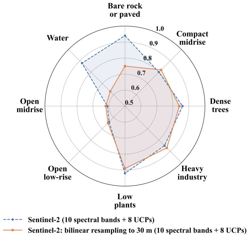
The resampled Sentinel-2 provides a more controlled indication of the role of spatial resolution. The overall metrics decrease from the original Sentinel-2 configuration to the resampled version, with OA dropping to 0.76 and both macro- and weighted F1-scores also reaching 0.76 (Figure 8). However, the class-wise results show that this effect is not uniform across LCZ classes. The strongest reductions are observed for bare rock or paved and water. This is an important result because these classes are usually spectrally distinctive, but they can be spatially fragmented or strongly affected by boundaries. At 10 m, Sentinel-2 can better capture narrow water bodies, paved surfaces, roads, and sharp transitions between artificial and natural surfaces. After resampling to 30 m, these features are spatially smoothed and more likely to be mixed with adjacent land-covers. As a result, their spectral signal becomes less pure, and the classifier loses part of the separability that was present at the original resolution. The observed response is consistent with previous LCZ studies showing that spatial resolution, mapping-unit size, and neighborhood context can substantially affect classification accuracy and the delineation of heterogeneous urban classes [22,29,43].

In contrast, dense trees and low plants show only moderate reductions. These vegetation classes remain relatively well classified after resampling, probably because they often occur in more spatially continuous patches and preserve a recognizable vegetation signal even at coarser resolution. However, the small decrease still indicates that vegetation separability can be affected by mixed pixels, especially along boundaries between tree cover, grass, agricultural areas, and urban vegetation.

The built-up classes show a different behavior, with compact midrise, heavy industry, open low-rise, and open midrise remaining broadly comparable between the original and resampled Sentinel-2 configurations, with only minor changes in F1-score. This suggests that the main limitations for these classes are not only pixel size but also their intrinsic morphological and spectral overlap. Open low-rise and open midrise are already difficult at 10 m because they contain mixed proportions of roofs, roads, vegetation, and open spaces. Resampling to 30 m does not substantially change this ambiguity, because the classes are already internally heterogeneous at the original resolution.

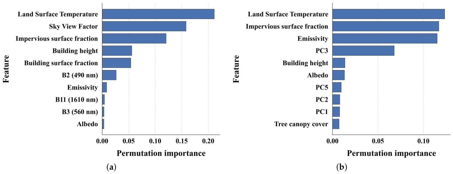
The feature-importance analysis shows that UCPs, such as impervious surface fraction, sky view factor, and land surface temperature, consistently rank among the most influential predictors. This supports the relevance of morphological and thermo-radiative descriptors for LCZ classification, suggesting that UCPs provide information that is complementary to spectral predictors, especially for classes whose separability depends on urban structure and surface properties [25,30]. The lower importance of emissivity in the Sentinel-2 configuration (Figure 9) may be partly attributed to its resampling to 10 m. In addition, some of the information it provides may have been redundant with the spectral bands and other UCPs. In the PRISMA configuration, where the analysis was conducted at 30 m spatial resolution, the different correlation structure among features may have allowed emissivity to provide a more distinct contribution. Absolute permutation-importance values should therefore be interpreted as model- and feature-space-specific and not as direct measures of physical relevance.

Although LCZ classes are primarily defined by surface structure, cover, and material properties, the spectral response of vegetation-related classes is season-dependent. The temporal mismatch between the Sentinel-2 and PRISMA images (due to the limited availability of PRISMA scenes covering the study area) may have affected the separability of dense trees and low plants, since the two scenes represent different seasonal and phenological conditions. It may also have influenced the optical contribution to the discrimination of mixed built-up classes, where vegetation, impervious surfaces, and building materials coexist within the same reference polygons. The relevance of acquisition season is supported by multi-seasonal LCZ studies, which have shown that temporal information improves the representation of vegetation and urban land-cover dynamics [45].

In addition, some UCP layers were not temporally synchronous with the satellite imagery. In particular, LST and albedo were derived from June to August 2019 composites and therefore represent warm-season thermo-radiative surface conditions rather than the instantaneous state of the scene at the time of image acquisition. Their use is consistent with the urban-climate objective of the study, because summer conditions are especially relevant for LCZ-based UHI analysis. However, this temporal mismatch may influence feature importance and classification behavior, especially where seasonal vegetation dynamics affect the relationship between spectral reflectance and thermo-radiative properties. Previous studies have also demonstrated that LCZ thermal behavior varies across seasons, supporting a cautious interpretation of thermo-radiative predictors derived from a different seasonal period [46].

5. Conclusions

This study evaluated a multi-source approach for fine-scale LCZ mapping in Bologna by combining Sentinel-2 and PRISMA imagery with urban canopy parameters and by examining how feature representation, spatial resolution, and training-sample heterogeneity affect classification performance.

The results showed that both baseline configurations achieved good classification performance on the unfiltered independent test set, with an OA of 0.79 for Sentinel-2 and 0.82 for PRISMA. The highest F1-scores were obtained for more homogeneous classes, such as dense trees, low plants, bare rock or paved, and water, whereas open low-rise and open midrise remained the most difficult classes to classify. This indicates that a major challenge in the study area is related to the heterogeneity of the urban fabric and the limited separability of structurally similar built-up LCZs.

Training-sample filtering produced limited changes in classification performance, with effects varying across sensors and classes. For Sentinel-2, the filtered models slightly improved the point estimates, with Z-score filtering providing the best performance among the tested strategies. For PRISMA, the response was more variable: Isolation Forest achieved the highest point estimates, while Z-score and IQR filtering reduced performance compared with the raw baseline. Since the polygon-level bootstrap CIs for the paired differences crossed zero in all cases, these changes should not be interpreted as stable accuracy improvements. The adopted approach proved to be useful for highlighting the sensitivity of LCZ classification to sample heterogeneity, mixed pixels, and class ambiguity.

The results obtained with Sentinel-2 and PRISMA data also showed that higher spectral dimensionality does not necessarily lead to better LCZ mapping. However, the comparison between Sentinel-2 and PRISMA, with the latter achieving slightly higher overall accuracy, must account for differences not only in spectral resolution but also in spatial resolution, acquisition date, and number of sampled pixels. The resampled Sentinel-2 further indicates that the effect of spatial resolution is class-dependent, with stronger reductions for bare rock or paved and water, while built-up classes remained broadly comparable between the original and resampled configurations.

Overall, the results indicate that LCZ classification performance is controlled by feature discriminative power, spatial resolution, urban morphology, sample heterogeneity, and class-specific separability. The feature relevance analysis proves the complementary importance of UCPs, which describe structural and thermo-radiative properties that are not fully represented by spectral information alone. Future work should focus on multi-seasonal acquisitions, explore systematic parameter optimization to identify class-specific configurations for handling heterogeneous samples that maximize classification performance, and assess the transferability of the workflow to other urban areas.