


Highlights
What are the main findings?
- A sequential Gaussian Process–Random Forest workflow was used for temporal gap filling and model-based spatial downscaling of GRACE-based groundwater-storage anomalies.
- The resulting 1 km gridded estimates showed temporal agreement with groundwater-level anomalies (R = 0.88) and identified persistent groundwater depletion in northern Henan.
What are the implications of the main findings?
- The workflow improves the temporal continuity and spatial representation of GRACE-based groundwater-storage estimates without implying independently observed groundwater information at the 1 km scale.
- The approach is potentially applicable to other regions, subject to local calibration, hydrogeological conditions, and validation with independent observations.
Abstract
Groundwater-storage anomalies (GWSA) derived from the Gravity Recovery and Climate Experiment (GRACE) mission provide valuable information for regional groundwater monitoring. Improving the spatial representation and temporal continuity of GRACE-derived GWSA is important for supporting groundwater assessment at subregional scales. A sequential framework combining Gaussian Process (GP) temporal gap filling and Random Forest (RF) spatial downscaling was developed for GWSA reconstruction in Henan Province, China, during 2002–2022. The GP model was used to reconstruct missing observations and characterize temporal variations, while the RF model statistically redistributed the GRACE-based GWSA signal using multi-source hydroclimatic predictors. The resulting dataset comprises model-derived GWSA estimates on a 1 km output grid constrained by the coarse spatial support of GRACE observations and the relationships learned from the auxiliary variables. Therefore, the 1 km grid spacing should not be interpreted as an independent 1 km resolving capability for groundwater-storage variations. Agreement with the parent GRACE-based GWSA product was used to assess coarse-scale reconstruction consistency rather than independent fine-scale accuracy. Comparison with groundwater-level anomalies from 63 monitoring wells yielded a correlation coefficient of 0.88, indicating temporal agreement at the sampled locations. Because the groundwater-level observations were not converted into storage anomalies using specific yield, this comparison does not establish absolute GWSA accuracy or independently validate the model-derived fine-scale spatial patterns. The reconstructed estimates revealed pronounced spatial heterogeneity in groundwater-storage changes, with persistent depletion concentrated in northern Henan, where groundwater decline rates exceeded 20 mm yr−1. Overall, the framework improved the temporal continuity and spatial representation of GRACE-based groundwater-storage estimates while retaining the fundamental spatial constraints of satellite gravimetry. The results demonstrate the potential of integrating GRACE observations, machine learning, and multi-source Earth observation data to support regional groundwater assessment.
1. Introduction
Groundwater is one of the most important freshwater resources supporting domestic consumption, agricultural irrigation, industrial production, and ecosystem sustainability worldwide [1]. In many arid and semi-arid regions, groundwater serves as the primary water source because of its relatively stable availability and favorable water quality. However, increasing groundwater withdrawal driven by population growth, agricultural intensification, and industrial development has resulted in widespread groundwater depletion and associated environmental problems, including land subsidence, groundwater funnel formation, and ecological degradation [2,3]. Effective monitoring of groundwater-storage dynamics is therefore essential for understanding regional water resource changes and supporting sustainable groundwater management [4].
Traditional groundwater monitoring mainly relies on in situ observation wells. Although these measurements provide relatively accurate local information, their sparse and uneven spatial distribution limits the characterization of groundwater variations at regional and basin scales [5]. In many regions, groundwater assessments are further constrained by insufficient monitoring networks and limited observational records [6]. The launch of the Gravity Recovery and Climate Experiment (GRACE) mission in 2002 and its successor GRACE Follow-On (GRACE-FO) mission in 2018 have provided a unique opportunity for monitoring terrestrial water storage changes from space [7]. Owing to its long-term observations and near-global coverage, GRACE has been widely applied to estimate terrestrial water storage and groundwater-storage anomalies (GWSA) at regional and continental scales [8,9,10,11]. Nevertheless, despite its unique capability for large-scale groundwater monitoring, the practical application of GRACE-derived groundwater products remains constrained by two major limitations: coarse spatial resolution and incomplete temporal observations. These limitations restrict their applicability for sub-regional groundwater assessment and motivate the development of advanced spatiotemporal reconstruction approaches.
For temporal analysis, gaps in GRACE and GRACE-FO observations are commonly reconstructed using interpolation-based methods or parametric models composed of long-term trends and harmonic terms. Linear and spline interpolation are straightforward for isolated missing months, but they may oversmooth long interruptions and provide no direct estimate of reconstruction uncertainty. Parametric trend–seasonal models preserve the dominant long-term and annual components but generally impose fixed functional forms, limiting their ability to represent temporally correlated departures from the prescribed trend and seasonal cycle. These limitations are particularly relevant to pixel-wise GRACE time series, which contain irregular missing months and the extended interruption between the GRACE and GRACE-FO missions. The GP formulation used in this study combines explicit linear and annual components in the mean function with a Matérn covariance function to model temporally correlated residual variations and to provide posterior means and predictive uncertainties for missing observations [12,13]. This study does not introduce a new GP algorithm beyond the reconstruction method previously presented by Xu et al. [14]. Instead, the added contribution is the pixel-wise application of that method to GRACE time series and its integration with subsequent RF-based spatial downscaling and residual correction. The GP component fills missing monthly observations but does not increase the native monthly temporal resolution of the GRACE/GRACE-FO product. The GP-reconstructed series therefore provides temporally continuous inputs for monthly spatial modeling, linking temporal gap filling and spatial downscaling within a sequential reconstruction workflow.
For spatial enhancement, numerous studies have explored statistical, hydrological, and machine learning approaches to improve the spatial resolution of GRACE observations. Ning et al. [15] developed an empirical regression model based on water balance relationships to downscale GRACE-derived water storage. Wan et al. [16] proposed a statistical framework that redistributed residual water storage components using hydrological information. Yin et al. [17] established relationships between evapotranspiration products and groundwater-storage anomalies to improve regional spatial representation. With the rapid development of machine learning techniques, nonlinear approaches such as Artificial Neural Networks (ANN) and Random Forest (RF) have demonstrated considerable potential in groundwater estimation and GRACE downscaling studies [18,19]. More recently, advances in remote sensing artificial intelligence have further improved the capability of extracting complex spatial patterns, modeling nonlinear feature interactions, and representing heterogeneous geospatial information from Earth observation data [20,21,22]. These developments indicate the strong potential of data-driven approaches for enhancing the spatial characterization of GRACE-derived groundwater products. In addition, machine learning-based downscaling methods integrated with feature selection and physical constraints have significantly improved the spatial representation of groundwater-storage variations [23,24,25,26,27,28,29,30,31,32].
Despite these advances, several challenges remain. Existing studies typically focus on either temporal reconstruction or spatial downscaling separately, while integrated spatiotemporal reconstruction frameworks are still relatively limited. Moreover, most existing studies have been conducted at continental, national, or large river-basin scales, whereas high-resolution characterization of groundwater dynamics at provincial and sub-regional scales remains insufficient. The complex temporal variability and spatial heterogeneity of groundwater systems are difficult to characterize simultaneously, which may introduce inconsistencies in reconstructed groundwater products. Therefore, there is a need for an integrated framework capable of jointly improving temporal continuity and spatial representation of GRACE-derived groundwater products.
Unlike previous studies that primarily addressed either temporal reconstruction or spatial downscaling, the present study evaluates how temporal gap filling affects subsequent spatial regression within a sequential regional workflow. The methodological contribution therefore lies not in proposing new GP, RF, or kriging algorithms, but in integrating these established components with pseudo-gap validation, component-wise ablation, repeated spatiotemporally blocked evaluation, and explicit assessment of parent-scale consistency. The study should consequently be regarded as a regional GWSA reconstruction and evaluation framework rather than a newly developed joint machine-learning model.
Henan Province, located in the North China Plain, has experienced substantial groundwater depletion owing to intensive agricultural irrigation, rapid urbanization, and increasing water demand. As one of the most important agricultural regions in China, the province provides an appropriate case for evaluating model-based groundwater-storage reconstruction approaches. To address the above challenges, this study develops a sequential workflow that combines Gaussian Process (GP) temporal gap filling with Random Forest (RF) spatial downscaling to reconstruct groundwater-storage anomalies during 2002–2022. The two components are trained independently rather than jointly optimized. First, the GP model is fitted to the GRACE time series to reconstruct missing monthly observations and provide temporally continuous GWSA inputs. The completed GWSA series are then used as the target data for training the RF model, which estimates statistical relationships between coarse-scale GWSA and multi-source hydroclimatic predictors. These relationships are subsequently applied to the corresponding 1 km predictor datasets to generate model-derived gridded estimates, followed by residual correction. Thus, the term “framework” refers to the integration of independently estimated temporal and spatial components within a sequential workflow and does not imply joint statistical estimation or end-to-end optimization.
The study addresses five research questions: (1) How accurately can GP reconstruct missing GRACE observations? (2) How well does RF generalize, and does GP-based gap filling improve its performance? (3) Do the downscaled estimates preserve the parent GRACE-scale signal? (4) How closely do the estimated GWSA variations agree temporally with groundwater-level anomalies from monitoring wells? (5) How are GWSA variations statistically associated with hydroclimatic variability, water use, and inter-basin water transfer? Accordingly, this study develops a sequential GP–RF workflow, generates model-derived GWSA estimates on a 1 km output grid constrained by GRACE observations, and evaluates temporal reconstruction, RF generalization, coarse-scale consistency, well-based temporal agreement, and associations with climatic and anthropogenic factors.
The remainder of this paper is organized as follows. Section 2 introduces the study area, datasets, and methodology. Section 3 presents the reconstruction results and validation analysis. Section 4 discusses the performance, advantages, and limitations of the proposed framework. Finally, conclusions are summarized in Section 5.
2. Methodology
2.1. Study Area
Henan Province is located in the mid-latitude region of central and eastern China, with geographic coordinates ranging from 31° to 36° north latitude and 110° to 116° east longitude (Figure 1a). The terrain generally slopes from west to east, surrounded by mountains on the south, west, and north sides. The central and eastern parts belong to the North China Plain region, while the southwest part constitutes the Nanyang Basin (Figure 1b). The climate is predominantly warm temperate, with the southern region transitioning into the subtropical zone, characterized by a continental monsoon climate transitioning from the North Subtropical Zone to the warm temperate zone, with a transition from plain to hilly and mountainous climates from east to west. The region experiences a continental monsoon climate, with an average temperature ranging from 12.1 to 15.7 °C from north to south across the province and an annual precipitation of 532.5 to 1380.6 mm. Rainfall is concentrated mainly from June to August, with distinct seasons, concurrent rain and heat, and frequent meteorological disasters [33]. Henan Province is one of the major grain-producing regions in northern China, grappling with longstanding issues of water scarcity and overexploitation of groundwater [34]. Concurrently, rapid industrial and agricultural development, coupled with population growth, have made water scarcity a critical factor influencing the region’s development [35]. Therefore, investigating the groundwater storage in this region holds significant practical importance and utility. In recent decades, due to intensive agricultural irrigation activities, groundwater resources have been overexploited in Henan Province, leading to severe groundwater depletion, deterioration in water quality, land subsidence, and a series of environmental issues that have significantly impeded the sustainable development of water resources. These characteristics make Henan Province an appropriate study area for evaluating GRACE-based groundwater-storage reconstruction and spatial downscaling.
Figure 1.
The study area (a) location; (b) Digital Elevation Model (DEM) and distributions of observation wells.
2.2. GP Reconstruction of GWSA Time Series
Gaussian Process regression was applied independently to the monthly GRACE time series at each distributed grid location to reconstruct missing observations. Let denote the observed equivalent water height at epoch . The observation model is expressed as:
where represents the deterministic temporal components, is a zero-mean latent Gaussian Process, and is independent Gaussian observation noise. Time was expressed in years relative to the first observation epoch:
where and are expressed in decimal years. Consequently, a period of one unit in t corresponds to one year.
The mean function contains an intercept, a linear trend, and annual harmonic terms:
where is the intercept, is the linear rate, and and describe the annual seasonal component. This formulation assumes a constant annual amplitude over the analysis period. The model does not explicitly estimate time-varying seasonal amplitudes; instead, temporally correlated departures from the prescribed trend and annual cycle are represented by the covariance function.
The latent process was modeled using a Matérn 3/2 covariance function:
where , is the temporal length scale, and is the process variance. The covariance matrix of the observations is therefore
where contains the covariance values calculated using Equation (4), is the n × n identity matrix, and represents independent observation-noise variance and unresolved short-timescale variability.
For n observed epochs and m missing epochs, let denote the observation vector, denote the prediction epochs, and denote the corresponding mean-function design matrices. The joint distribution of the observations and latent values at the missing epochs is
where is the covariance matrix between the observed and prediction epochs, and is the covariance matrix among the prediction epochs. Here, , , , and . Moreover, , , , and .
The posterior mean and covariance at the missing epochs are
and
The posterior mean was used to fill the missing observations. Epoch-specific 95% predictive intervals were calculated from the posterior predictive variance. The predictive variance was computed from the fitted GP model, in which the observation-noise variance was incorporated through the covariance matrix defined in Equation (5). The resulting temporal uncertainty was evaluated in the GP reconstruction stage but was not propagated through the subsequent RF downscaling and residual-correction stages; this limitation is addressed in the Discussion.
The GP models were implemented in MATLAB R2025a using the fitrgp function with exact fitting and prediction, a Matérn 3/2 kernel, and QR-based matrix computation. The initial values were set to for the four mean-function coefficients, 1 year for the temporal length scale, 1 mm for the process standard deviation, and 1 mm for the observation-noise standard deviation. The parameters were estimated by maximizing the marginal log-likelihood using a quasi-Newton optimizer:
This procedure represents empirical Bayes, or type-II maximum-likelihood estimation, because point estimates of the hyperparameters were obtained rather than samples from their full posterior distributions.
2.3. RF-Based Spatial Downscaling of GWSA
Random Forest regression was used to establish statistical relationships between monthly groundwater-storage anomalies and multi-source hydroclimatic variables at the coarse GRACE sampling scale. For coarse sampling cell i and month t, the target variable was defined as
where TWSA is the GP-completed GRACE/GRACE-FO terrestrial water storage anomaly, and SMSA, SWEA, and CWSA denote soil-moisture-storage anomaly, snow-water-equivalent anomaly, and canopy-water-storage anomaly, respectively. The monthly GWSA target was used in its original anomaly form without detrending or normalization.
The predictor vector was defined as
where P, ET, T, , , and NDVI represent monthly precipitation, evapotranspiration, air temperature, daytime land-surface temperature, nighttime land-surface temperature, and normalized difference vegetation index, respectively. Spatial coordinates, elevation, explicit month or season indicators, and lagged variables were not included. Because Random Forest regression is insensitive to monotonic differences in predictor scale, the input variables were not standardized.
The original predictor datasets were available on a 1 km grid. For coarse-scale model training, they were aggregated to the 0.25° GRACE sampling grid using pixel averaging. Each valid grid-cell–month combination formed one sample. The resulting samples were arranged into a predictor matrix and a target vector , where N denotes the number of valid grid-cell–month samples. Samples containing missing values in the target or any predictor were excluded.
The RF configuration was optimized through grid search. The number of trees was selected from {100,200,300,500}, the minimum leaf size from {1,2,4,8}, the maximum tree depth from {10,20,30}, and the number of candidate predictors considered at each split from {2,3,4,6}. Bootstrap sampling fractions of {0.7,0.8,1.0} were also evaluated. The selected model consisted of 300 regression trees, a minimum leaf size of 2, a maximum depth of 20, and three randomly selected candidate predictors at each split. Bootstrap sampling was enabled, with 80% of the training samples drawn for each tree. The random seed was fixed at 42 to ensure reproducibility.
Hyperparameter combinations were evaluated using fivefold spatially blocked cross-validation. The 0.25° samples were grouped into approximately 1° × 1° spatial blocks, and all monthly records belonging to the same spatial block were assigned to the same fold. Thus, observations from the same coarse spatial support were not shared between the training and validation subsets. The parameter combination yielding the lowest mean validation RMSE was selected, while the correlation coefficient and Nash–Sutcliffe efficiency were used as supplementary metrics. In addition, temporal generalization was assessed using 2002–2017 as the training period and 2018–2022 as an independent temporal test period.
After the RF model was trained at the coarse scale, it was applied to the corresponding 1 km predictor datasets:
where j denotes a 1 km output grid cell and is the initial model-derived GWSA estimate.
This procedure assumes that the statistical relationships learned between GWSA and the selected hydroclimatic variables at the coarse scale remain sufficiently stable when applied to the 1 km predictor data. However, local groundwater variations may also be controlled by aquifer properties, groundwater abstraction, irrigation infrastructure, river–aquifer interactions, and other processes that are not represented by the selected predictors. The scale-transfer assumption may therefore be less valid in areas with substantial local hydrogeological or anthropogenic heterogeneity. Accordingly, the resulting 1 km estimates are interpreted as model-derived spatial redistributions of the GRACE-constrained signal rather than as independently observed or physically resolved groundwater-storage variations at the 1 km scale.
For benchmark comparison, multiple linear regression and support vector regression replaced only the RF regression component, while the GP-based temporal reconstruction was retained in all workflows. The three workflows are therefore referred to as GP–MLR, GP–SVR, and GP–RF. They used the same GP-completed monthly GWSA target, the same six hydroclimatic predictors, identical valid grid-cell–month samples, and identical spatial and temporal partitions. MLR was fitted by ordinary least squares with an intercept. SVR used a radial-basis-function kernel, with C = 50, γ = 0.10, and , selected from , and . SVR predictors were standardized using statistics calculated only from the corresponding training subset. All benchmark metrics were calculated before residual correction. Generalization performance was evaluated using 20 repeated spatiotemporally blocked splits. In each repetition, approximately 20% of the spatial blocks and one contiguous four-year period were withheld for testing, while model selection was conducted using fivefold blocked cross-validation within the remaining training data. Identical partitions were used for all three workflows, and performance was summarized as the mean and standard deviation across the repeated test splits.
RF prediction uncertainty was characterized empirically using the variability of out-of-sample performance across the 20 repeated spatiotemporally blocked test splits. The reported standard deviations represent the sensitivity of model performance to different held-out spatial domains and temporal periods; they do not constitute cell-specific prediction intervals or a complete uncertainty estimate for the final 1 km product.
2.4. Datasets and Preprocessing
The datasets used in this study are summarized in Table 1. All analyses were conducted for January 2002–December 2022. The groundwater-level dataset originally covers 2005–2018; however, the well-based comparison was restricted to January 2005–December 2017 because the records available for 2018 were incomplete and temporally inconsistent among the selected wells. All raster datasets were reprojected to the WGS 84 geographic coordinate system. Continuous variables were resampled using bilinear interpolation when reprojection was required, whereas area-weighted averaging was used to aggregate the 1 km predictors to the 0.25° GRACE sampling grid.
Table 1.
Datasets used in this study and their preprocessing.
2.4.1. GRACE and GRACE-FO Terrestrial Water Storage Anomalies
Monthly terrestrial water storage anomalies were obtained from the CSR GRACE/GRACE-FO RL06 Mascon solution [36,37]. The distributed product is sampled on a 0.25° grid, corresponding to approximately 27–28 km in latitude at the equator. However, the underlying CSR mascons have an effective spatial support of approximately 120 km, and adjacent 0.25° grid values should not be interpreted as independent observations.
The provider-supplied degree-1, C20, C30, glacial isostatic adjustment, atmospheric and ocean de-aliasing, and ellipsoidal-Earth corrections were retained. No additional spatial scaling factors, coastline filters, or regional averaging kernels were applied in this study. Although the mascon processing reduces leakage relative to unconstrained spherical-harmonic solutions, residual leakage and spatial correlation remain and are considered sources of uncertainty.
No additional empirical bias correction was applied between GRACE and GRACE-FO because both mission periods were taken from the same harmonized CSR processing series. The GP model was used only to reconstruct missing monthly observations, including the interruption between the two missions.
The CSR TWSA values, originally expressed in centimeters of equivalent water height, were converted to millimeters. The anomaly baseline was the January 2004–December 2009 temporal mean supplied with the CSR product.
2.4.2. GLDAS Storage Components and GWSA Calculation
Monthly land-surface storage components were obtained from the GLDAS-2.1 Noah monthly product, GLDAS_NOAH025_M_2.1, which is part of the Global Land Data Assimilation System (GLDAS) [38]. Soil-moisture storage was calculated as the sum of the four Noah soil layers:
where the subscripts indicate soil depth in centimeters. Snow water equivalent and canopy-interception storage were obtained from the corresponding GLDAS variables. All three components were expressed in kg m−2 and converted to millimeters of equivalent water thickness using .
For each grid cell, the storage anomalies were calculated relative to the cell-specific January 2004–December 2009 means:
where X represents soil moisture, snow water equivalent, or canopy water storage; B is the baseline period; and is the number of valid baseline months.
GWSA was calculated as
where SMSA, SWEA, and CWSA denote soil-moisture-storage, snow-water-equivalent, and canopy-water-storage anomalies, respectively.
Surface-water storage in rivers, lakes, reservoirs, canals, and temporary floodwater was not independently estimated and removed. Consequently, the calculated GWSA may contain residual surface-water signals. This limitation is particularly relevant during the 2021 extreme-rainfall event and when interpreting temporal changes associated with the South-to-North Water Diversion Project. These events are therefore discussed as temporal associations rather than as direct evidence of groundwater-storage causation.
2.4.3. MODIS and Meteorological Predictors
NDVI was obtained from the MODIS/Terra Vegetation Indices Monthly L3 Global 1 km product, MOD13A3 Collection 6.1. The NDVI scale factor of 0.0001 was applied. Pixels flagged as invalid, snow/ice, cloud-contaminated, or affected by poor retrieval quality were excluded according to the product quality-assurance layer. Because MOD13A3 is already a calendar-month product, no additional temporal aggregation was conducted.
Daytime and nighttime land-surface temperatures were obtained from the MODIS/Terra Land Surface Temperature/Emissivity 8-Day L3 Global 1 km product, MOD11A2 Collection 6.1. The scale factor of 0.02 K was applied, and temperatures were converted from kelvin to degrees Celsius. Only pixels satisfying the mandatory quality criteria and an estimated LST error of no more than 2 K were retained. Valid 8-day composites were converted to monthly means using weights proportional to the number of days overlapping each calendar month.
Evapotranspiration was obtained from the gap-filled MODIS/Terra Net Evapotranspiration 8-Day L4 Global 500 m product, MOD16A2GF Collection 6.1. Evapotranspiration-related variables have been widely used in regional water-balance and groundwater studies because they represent an important component of land-surface-water exchange [39]. The ET scale factor was applied, and the values were converted to millimeters of water equivalent. When an 8-day composite overlapped two months, its value was allocated proportionally according to the number of days falling within each month. Monthly ET was calculated by summing the apportioned values and was then aggregated from 500 m to the common 1 km grid using area-weighted averaging.
For the MODIS products, monthly values were retained only when at least 50% of the corresponding monthly observations passed the quality-control criteria. Isolated missing months of no more than two consecutive months were filled by linear temporal interpolation; longer gaps were retained as missing and excluded from RF sample construction.
Monthly precipitation and air temperature were obtained from the “1 km Monthly Precipitation Dataset for China” and the “1 km Monthly Mean Temperature Dataset for China,” respectively, provided by the National Tibetan Plateau/Third Pole Environment Data Center. Both products have a spatial interval of 0.008333° and were developed by downscaling CRU time-series data using WorldClim climatology and station-based evaluation. Precipitation was expressed in mm month−1 and temperature in °C.
All predictor datasets were aligned to the same monthly calendar and geographical extent. The 1 km predictor grids were aggregated to the 0.25° training grid using area-weighted averages, excluding missing pixels from the denominator.
2.4.4. Groundwater-Level Observations
Groundwater observations were obtained from the “Danjiangkou Reservoir Dynamics and North China Plain Groundwater Level Dataset (2005–2018)” provided by the National Earth System Science Data Center. The dataset contains groundwater burial-depth observations from monitoring wells. Burial depth was converted to groundwater level using the corresponding ground-surface elevation, and groundwater-level anomalies were calculated by subtracting the temporal mean of each well.
The following criteria were used to select the monitoring wells: (1) the well was located within Henan Province; (2) at least 60 valid monthly observations were available during 2005–2017; (3) the missing-data proportion did not exceed 20%; (4) no continuous missing interval exceeded 12 months; (5) isolated gaps of no more than two months were linearly interpolated; (6) potential outliers were detected using a seven-month Hampel filter with a threshold of three median absolute deviations and were subsequently checked against adjacent observations; (7) wells with abrupt, unsupported level shifts or unresolved datum changes were excluded.
After quality control, 63 wells were retained. Because coverage in 2018 was incomplete and differed substantially among wells, the common validation period was restricted to January 2005–December 2017.
Specific-yield data with sufficient spatial coverage were unavailable; therefore, groundwater-level anomalies were not converted to groundwater-storage anomalies. The well comparison was used only to evaluate temporal consistency between the estimated GWSA and groundwater-level variations at the sampled locations. It does not constitute validation of absolute GWSA magnitude or independent validation of the complete 1 km spatial pattern.
For the benchmark well comparison, the final model-derived estimates from GP–MLR, GP–SVR, and GP–RF were extracted from the 1 km output cells containing the same 63 monitoring wells. All workflows were evaluated using identical well locations, paired months, groundwater-level anomaly definitions, and residual-correction procedures during January 2005–December 2017.
Model performance was evaluated using the root mean square error (RMSE), Pearson correlation coefficient (R), and Nash–Sutcliffe efficiency (NSE):
where and denote the reference and model-estimated values for sample i, respectively; and are their corresponding sample means; and N is the number of paired samples. In the pseudo-gap experiments, represents the artificially withheld GRACE/GRACE-FO value. In the regression-model evaluation, represents the GP-completed coarse-scale GWSA target. For comparison with groundwater-level anomalies, only R was calculated because the well observations were not converted to groundwater-storage units.
2.5. Workflow and Residual Correction
The proposed workflow consisted of GP-based temporal gap filling, GWSA derivation, RF-based spatial downscaling, monthly residual correction, and assessment of consistency with the parent GRACE signal (Figure 2).
Figure 2.
The overall technical route flowchart for improved spatiotemporal estimation of GWSA.
First, the GP model was fitted independently to the monthly GRACE/GRACE-FO time series at each distributed 0.25° grid location. The GP reconstruction was therefore conducted pixel-by-pixel rather than using a spatially averaged regional time series. The GP model included only a temporal covariance function and did not explicitly account for spatial covariance among neighboring grid locations. Because adjacent grid cells in the distributed CSR product are spatially correlated and may represent the same or neighboring native mascon support, the reconstructed grid-cell series were not treated as spatially independent observations. The absence of an explicit joint spatiotemporal covariance structure is acknowledged as a limitation.
The GP-completed TWSA was converted to GWSA using Equation (15). The hydroclimatic predictors were aggregated to the 0.25° sampling grid to train the RF model, which was subsequently applied to the original 1 km predictor datasets according to Equation (12) to generate initial model-derived GWSA estimates.
Residual correction was conducted independently for each month on the 0.25° distributed CSR sampling grid. The procedure did not use the boundaries of the underlying native CSR mascons. For month t, the initial 1 km RF estimates were aggregated to each 0.25° distributed grid cell using area-weighted averaging:
where i denotes a 0.25° distributed CSR grid cell, j denotes a 1 km output cell overlapping grid cell i, and is the fractional area of the overlapping portion of cell j, normalized by the total valid overlapping area within grid cell i. Partial overlaps along the boundaries of the 0.25° cells were calculated from the intersected areas in the common WGS 84 coordinate system.
The monthly residual on the distributed sampling grid was defined as
A positive residual, therefore, indicates that the aggregated RF estimate underestimated the GRACE-based GWSA value at the corresponding 0.25° distributed grid cell. The residual field was interpolated separately for each month from the 0.25° grid to the 1 km output grid using ordinary kriging. Month-specific residual fields were used, and no temporally averaged residual surface was applied throughout the study period.
The preliminary residual-corrected estimate was calculated as
where denotes the month-specific interpolated residual at 1 km grid cell j.
To assess consistency with the distributed GRACE product, the residual-corrected estimates were reaggregated to the 0.25° grid:
The remaining reaggregation difference was calculated as
where an explicit distributed-grid consistency adjustment was applied, the final estimate was expressed as
which ensures that
apart from numerical and boundary-weighting errors.
Agreement after reaggregation is therefore interpreted as consistency with the 0.25° distributed CSR product rather than independent validation at the native mascon support or at the 1 km scale. Because adjacent values in the 0.25° distributed product remain spatially correlated and are constrained by the underlying approximately 120 km mascon support, the resulting grid-cell comparisons should not be interpreted as independent observations.
3. Results and Analysis
3.1. Data Gap Filling and Trend Estimation of GWS
The GP model was fitted independently to each GRACE grid-cell time series to reconstruct missing monthly observations. Figure 3 illustrates the pixel-level GP reconstruction during the interruption between the GRACE and GRACE-FO missions, while Figure 4 presents the corresponding reconstruction of the regional TWSA time series. These results demonstrate the temporal continuity produced by the GP model but, by themselves, do not provide an independent assessment of reconstruction accuracy.
Figure 3.
GP-based gap-filling between GRACE and GRACE-FO at the pixel level.
Figure 4.
GP-based gap-filling in TWSA time series.
To evaluate the reconstruction performance independently, pseudo-gap experiments were conducted by temporarily withholding available GRACE observations. Three categories of missing-data scenarios were considered. First, 5%, 10%, and 20% of the available monthly observations were randomly omitted. Second, contiguous gaps of 3 and 6 months were introduced at randomly selected positions. Third, an 11-month contiguous gap was introduced to approximate the interruption between the GRACE and GRACE-FO missions. Each scenario was repeated 30 times using different gap locations.
The GP reconstruction was compared with linear interpolation, cubic-spline interpolation, harmonic regression, and Kalman smoothing. All methods were fitted using the same retained observations and evaluated against the same withheld GRACE values. Reconstruction performance was assessed using RMSE, MAE, correlation coefficient, and NSE. The empirical coverage of the GP 95% prediction intervals was also evaluated. Detailed results are presented in Table 2.
Table 2.
RMSE of the GP model and baseline methods for reconstructing artificially withheld GRACE/GRACE-FO TWSA observations under different pseudo-gap scenarios.
Detailed results for the pseudo-gap experiments are summarized in Table 2. Across all six scenarios, the GP model achieved the lowest average RMSE of 6.9 mm, compared with 9.5 mm for linear interpolation, 9.3 mm for cubic-spline interpolation, 10.9 mm for harmonic regression, and 7.7 mm for Kalman smoothing. The GP model also yielded an average MAE of 5.3 mm, a mean correlation coefficient of 0.94, and a mean NSE of 0.86. Its 95% prediction intervals achieved an average empirical coverage of 93.4%. For the 11-month contiguous gap approximating the GRACE–GRACE-FO interruption, the GP RMSE was 10.2 mm, lower than those of linear interpolation, cubic-spline interpolation, harmonic regression, and Kalman smoothing.
Overall, these results demonstrate that the GP model provides stable reconstruction performance across a range of gap lengths while maintaining reliable uncertainty estimates. The consistent performance in the pseudo-gap experiments supports the use of the GP-completed GWSA series as the temporal input for the subsequent RF downscaling.
In addition to the pseudo-gap experiments, the GP-completed TWSA series was compared with GLDAS-derived land-water-storage variations and the GRACE-based reconstruction of Rateb et al. [40] and the GRACE/GLDAS-based analysis of Syed et al. [41], as shown in Figure 5. Because GLDAS does not include groundwater storage and the Rateb product is also reconstructed from GRACE observations, neither dataset was treated as independent ground truth. The three series were detrended only to compare seasonal and interannual fluctuations during the missing-data period. Figure 5 therefore provides a qualitative assessment of short-term temporal consistency rather than evidence of long-term-trend reconstruction or absolute missing-value accuracy.
Figure 5.
Comparison of GP model filling results with other datasets. The red dotted box shows the fill-in missing gap between GRACE and GRACE-FO.
Using the GP-completed series for 2002–2022, the regional GWSA trend was estimated using ordinary least squares (OLS) linear regression, where monthly GWSAs were regressed against time. The estimated trend was −6.50 ± 1.3 mm/yr−1, compared with −7.75 ± 2.2 mm/yr−1 obtained using the conventional trend–seasonal model. The uncertainty represents the standard error of the fitted linear trend. The standard error of the estimated trend was 40.9% lower, while the in-sample residual RMSE decreased from 33.8 to 4.8 mm, corresponding to an 85.8% reduction. These percentages describe differences in model-fitting diagnostics for the observed months and are not interpreted as independent improvements in missing-value reconstruction accuracy.
Because groundwater-storage time series contain seasonal variability and temporal persistence, the uncertainty estimates based on linear regression errors may not fully account for autocorrelation effects. Therefore, the reported uncertainty should be interpreted as regression-based uncertainty, and potential impacts of temporal autocorrelation are acknowledged as a limitation.
The city-scale trends derived from the GP-completed GWSA series are reported in Table 3 and illustrated in Figure 6. The provincial trend reported in this study was calculated as the area-weighted average of the reconstructed grid-cell trends across Henan Province, whereas the values listed in Table 3 represent city-level averages for individual administrative units. Therefore, the arithmetic mean of the city-level trends is not expected to be identical to the provincial trend because the cities differ substantially in spatial extent and are not equally weighted in the provincial estimate. Most cities exhibited declining groundwater storage during 2002–2022. The strongest declines occurred in Anyang, Hebi, Puyang, and Xinxiang, with estimated rates exceeding 20 mm yr−1. Jiaozuo also exhibited a pronounced decline of approximately 19 mm yr−1. In contrast, Nanyang and Xinyang showed relatively stable long-term trends. These results describe the estimated spatial distribution of groundwater-storage trends, whereas their potential hydroclimatic and anthropogenic associations are examined separately in Section 3.3.
Table 3.
Long-term trend estimates for the 18 cities in Henan Province.
Figure 6.
Long-term trend change characteristics of GWSA across 18 cities in Henan Province from 2002 to 2022.
3.2. Fine Estimation of GWSA Spatial Distribution
The hydroclimatic predictor variables were first aggregated to the 0.25° GRACE sampling grid and used to train the RF model. The RF predictions were then compared with the GRACE-derived GWSA at the same sampling scale. As shown in Figure 7a,b, the RF estimates reproduced the broad spatial gradient of the GRACE-derived trends but showed moderate underestimation in several areas. The differences between the GRACE-derived GWSA and the RF estimates at the parent scale were subsequently used for residual correction. Figure 7c presents the long-term trend of the final model-derived GWSA estimates on the 1 km output grid. After residual correction and reaggregation, the estimates preserved the broad magnitude and spatial pattern of the parent GRACE-based signal. However, this agreement is an expected consequence of the residual-correction and coarse-scale consistency procedures and should not be interpreted as independent validation of the 1 km spatial patterns. The finer-scale variations shown in Figure 7c represent a model-derived spatial redistribution of the coarse GRACE signal based on the hydroclimatic predictor relationships and interpolated residuals. They provide additional spatial detail within the parent GRACE support, but their local accuracy cannot be established solely from their agreement with the GRACE-derived field used to construct the correction.
Figure 7.
Trends of GWSA. (a) Original GWSA. (b) Predicted GWSA. (c) Residual-corrected downscaled GWSA at 1 km resolution.
The coarse-scale performance of the RF-only estimates and the residual-corrected estimates was evaluated against the parent GRACE-derived GWSA. Figure 8 illustrates the comparison between the parent GRACE-derived GWSA and the final residual-corrected downscaled estimates. Before residual correction, the RF-only model achieved an MAE of 41.6 mm, an RMSE of 54.08 mm, an NSE of 0.758, and a correlation coefficient of 0.890. These statistics represent the predictive contribution of the hydroclimatic variables and the RF model without reintroducing information from the parent-scale residual field. After residual correction, the corresponding statistics were an MAE of 1.41 mm, an RMSE of 1.95 mm, an NSE of 0.99, and a correlation coefficient of 0.99. The substantial reduction in error primarily reflects the addition of residuals calculated from the same GRACE-derived GWSA and the resulting enforcement of coarse-scale consistency. Therefore, the post-correction statistics are interpreted as measures of reconstruction consistency with the parent GRACE signal rather than independent validation of local 1 km accuracy. The RF-only results demonstrate that the selected hydroclimatic predictors contain information relevant to the broad temporal variability of GWSA, whereas the residual-correction step restores the unresolved parent-scale component. Neither the close post-correction agreement nor the improvement relative to the RF-only estimates independently verifies the fine-scale spatial patterns within individual GRACE mascons.
Figure 8.
Comparison between the parent GRACE-derived GWSA product and the final residual-corrected downscaled GWSA estimates at the parent GRACE sampling scale. The reported statistics quantify the agreement between the residual-corrected downscaled estimates and the parent GRACE-derived GWSA product. These statistics describe coarse-scale consistency and do not constitute independent validation of local 1 km accuracy.
Figure 9 presents the model-derived annual mean GWSA estimates on the 1 km output grid for 2002–2021. These estimates were generated by applying the RF model to the fine-scale hydroclimatic predictors and subsequently imposing residual correction and consistency with the parent GRACE/GRACE-FO signal. Therefore, the spatial detail displayed in Figure 9 represents a model-based redistribution of the coarse-scale GWSA signal and should not be interpreted as direct observation or independent physical resolution of groundwater-storage variations at 1 km. The annual estimates indicate an overall decline in GWSA across Henan Province during the study period. Relatively low values were observed in 2002–2003, followed by an increase from 2004 to 2007. After approximately 2008, GWSA generally decreased, with the most persistent negative anomalies concentrated in northern Henan. Compared with 2020, the higher GWSA estimates in 2021 coincided with exceptionally high precipitation and the extreme rainfall event that affected Zhengzhou and surrounding areas in July 2021. However, because the present analysis does not formally separate precipitation recharge, temporary surface-water storage, and other hydrological processes, this temporal coincidence is not interpreted as direct evidence that the flood caused the estimated GWSA increase. Similarly, the persistent negative GWSA estimates in northern Henan were spatially consistent with areas characterized by intensive agricultural irrigation and high groundwater use. Previous regional information indicates that groundwater utilization exceeds 70% at the provincial scale and can exceed 80% in parts of the northern and eastern plains, where groundwater-depression cones have also been reported in the Anyang–Puyang–Hebi–Xinxiang region [42]. These contextual observations are consistent with the estimated depletion pattern, but they do not independently establish agricultural irrigation or groundwater abstraction as the sole causes of the model-derived spatial trends.
Figure 9.
Model-derived annual mean GWSA estimates on the 1 km output grid in Henan Province from 2002 to 2021. The estimates are constrained by the parent GRACE/GRACE-FO signal and should not be interpreted as independently observed groundwater-storage variations at an effective spatial resolution of 1 km.
Groundwater-level observations from 63 monitoring wells during January 2005–December 2017 were used to assess the temporal consistency of the model-derived GWSA estimates. For each well, the Pearson correlation coefficient was calculated between the monthly groundwater-level anomaly and the GWSA estimate from the corresponding 1 km output grid cell. Because the groundwater-level observations were not converted to storage anomalies using specific yield, this comparison evaluates temporal consistency rather than absolute groundwater-storage accuracy.
The well-specific correlation coefficients ranged from 0.14 to 0.91, with a median of 0.67 and an interquartile range of 0.55–0.78. Of the 63 wells, 52 wells, corresponding to 82.5%, had correlation coefficients greater than 0.50. After accounting for temporal autocorrelation, 55 of the 63 well-specific correlations were statistically significant at the 0.05 level. Figure 10 shows the spatial distribution of the well-specific correlation coefficients. The relatively high correlations were concentrated mainly in northern Henan, where most monitoring wells were located.
Figure 10.
Spatial distribution of well-specific Pearson correlation coefficients between monthly groundwater-level anomalies and model-derived GWSA estimates from the corresponding 1 km output grid cells during 2005–2017. Correlation significance was assessed using an effective sample size adjusted for temporal autocorrelation.
Figure 10 compares the regional mean groundwater-level anomaly from the 63 wells with the mean model-derived GWSA for the corresponding grid cells. The correlation coefficient between the two regional mean series was 0.88. This regional correlation summarizes the common temporal variability of the two datasets but was not used as the sole measure of model performance because it may be influenced by the shared long-term decline and the uneven spatial distribution of the monitoring wells.
To evaluate the contribution of the common long-term trend, the groundwater-level and GWSA series were independently detrended at each well before recalculating their correlations. After detrending, the well-specific correlations ranged from −0.06 to 0.78, with a median of 0.48 and an interquartile range of 0.34–0.60. A total of 41 wells remained significantly correlated at the 0.05 level after adjustment for temporal autocorrelation. The correlation between the detrended regional mean series was 0.62. The reduction from the original correlation results indicates that the common long-term decline contributed to the raw correlations, while the remaining correlations show that the model-derived GWSA also captured part of the seasonal and interannual groundwater-level variability.
Statistical significance and confidence intervals were calculated using an autocorrelation-adjusted effective sample size. For each well, the effective sample size was estimated from the lag-1 autocorrelations of the groundwater-level and GWSA series:
where N is the number of paired monthly observations and and are the corresponding lag-1 autocorrelation coefficients. Two-sided significance tests and 95% confidence intervals were then calculated using rather than the nominal number of monthly observations.
Overall, the well comparison indicates moderate-to-strong temporal agreement at most sampled locations, although the strength of this agreement decreases after removal of the common long-term trend. These results should therefore be interpreted as evidence of temporal consistency at the monitoring locations, not as independent validation of absolute GWSA magnitude or of the complete 1 km spatial pattern.
Figure 10 presents the spatial distribution of the well-specific correlations between monthly groundwater-level anomalies and the model-derived GWSA estimates at the corresponding 1 km output grid cells.
Figure 11 presents the temporal evolution of the regional mean groundwater-level anomaly and the mean model-derived GWSA at the 63 monitoring locations during January 2005–December 2017. For monitoring well k, groundwater burial depth was first converted to groundwater level as
where is the ground-surface elevation and is the observed groundwater burial depth. Groundwater-level anomalies were then calculated independently for each well:
where is the mean groundwater level of well k over its valid observations during the common comparison period. Through this conversion, positive groundwater-level anomalies indicate a rise in groundwater level; therefore, no additional post hoc sign reversal was applied.
Figure 11.
Regional mean monthly groundwater-level anomalies from 63 monitoring wells and model-derived GWSA estimates at the corresponding grid cells during 2005–2017. The two series are presented in their original units for comparison. The reported correlation coefficient (R = 0.88) was calculated using the paired anomaly series, and the detrended regional mean correlation was R = 0.62.
The regional groundwater-level series was calculated by averaging the well-specific anomalies for each month, and the corresponding regional GWSA series was calculated by averaging the model-derived GWSA values at the grid cells containing the monitoring wells. Only months with paired groundwater-level and GWSA estimates were included. The Pearson correlation coefficient was calculated from the unstandardized and nondetrended regional mean anomaly series. No min–max normalization or additional amplitude adjustment was applied when calculating the correlation.
The two regional mean series yielded a correlation coefficient of R = 0.88. For visual comparison in Figure 11, the two series were expressed as standardized anomalies with zero mean and unit standard deviation; this standardization does not affect their correlation coefficient. Because specific yield was not available, differences in amplitude between groundwater-level and storage anomalies were not interpreted quantitatively.
The raw regional correlation partly reflects the common long-term decline in northern Henan. After independently removing the linear trends from the two regional mean series, the correlation decreased to R = 0.62. Thus, the comparison indicates that the model-derived GWSA captured both a shared long-term tendency and part of the shorter-term seasonal and interannual variability. Figure 10 and Figure 11 represent complementary spatial and temporal summaries of the same well-based temporal-consistency assessment, rather than independent validation experiments.
To determine whether the relative performance identified by the grid-based evaluation was also supported by the monitoring-well observations, GP–MLR, GP–SVR, and GP–RF were compared using the same 63 wells and paired monthly records during January 2005–December 2017. As shown in Table 4, GP–RF achieved the strongest temporal agreement with the groundwater-level anomalies. Its median well-specific correlation was 0.67, compared with 0.61 for GP–SVR and 0.54 for GP–MLR. Correlations exceeded 0.50 at 52 wells for GP–RF, 44 wells for GP–SVR, and 35 wells for GP–MLR.
Table 4.
Temporal agreement between groundwater-level anomalies and model-derived GWSA estimates from the benchmark workflows at 63 monitoring wells during January 2005–December 2017.
The corresponding regional mean correlations were 0.88, 0.82, and 0.76 for GP–RF, GP–SVR, and GP–MLR, respectively. After independently removing the long-term trend from the groundwater-level and model-derived series, the regional correlations decreased to 0.62, 0.51, and 0.41, respectively. The reduction after detrending indicates that part of the raw agreement was associated with the common long-term variation. Nevertheless, GP–RF retained the highest temporal agreement under both the original and detrended comparisons.
Because the groundwater-level observations were not converted to groundwater-storage anomalies using specific yield, these results evaluate temporal covariation rather than agreement in storage magnitude. They also do not independently validate the complete fine-scale spatial patterns of the three model-derived products.
3.3. GWSA Analysis
Precipitation is an important potential source of groundwater recharge, although the relationship between precipitation and GWSA may also be affected by evapotranspiration, surface runoff, soil-water storage, groundwater abstraction, and delayed infiltration. Figure 12a presents the original monthly regional mean precipitation and model-derived GWSA series for Henan Province during 2002–2022.
Figure 12.
Temporal associations between regional mean GWSA and potential explanatory variables. (a) Monthly GWSA and precipitation series; (b) GWSA and water supplied through the South-to-North Water Diversion project. The temporal correspondence shown in panel (b) is descriptive and does not establish a causal effect of transferred-water supply on GWSA. A lagged-correlation analysis was conducted to quantify the temporal association between precipitation and GWSA. Before calculating the correlations, the linear trend was removed independently from each series, and the seasonal cycle was removed by subtracting the corresponding calendar-month climatological mean. The resulting deseasonalized anomalies were standardized to zero mean and unit standard deviation.
Pearson cross-correlations were calculated for lags from −12 to +12 months:
where and are the detrended and deseasonalized precipitation and GWSAs, respectively. A positive lag L indicates that precipitation precedes the corresponding GWSA variation. Uncertainty was evaluated using 2000 moving-block bootstrap realizations with a block length of 12 months, thereby retaining the principal temporal dependence within the monthly series.
The complete lagged-correlation results are reported in Table 5. The maximum correlation occurred when precipitation led GWSA by two months, with r = 0.52 and a 95% bootstrap confidence interval of 0.39–0.63. A similarly strong correlation was obtained at a three-month lag, with r = 0.49 and a 95% confidence interval of 0.35–0.60. Correlations decreased at longer positive lags and became statistically indistinguishable from zero after approximately six months.
Table 5.
Cross-correlation between detrended and deseasonalized monthly precipitation and regional mean GWSAs at different temporal lags.
These results indicate that the strongest statistical association occurred when precipitation preceded GWSA variations by approximately two to three months. Because the confidence intervals at the two- and three-month lags overlap, the analysis does not support identification of a single exact response time. The inferred lag is interpreted as a regional temporal association consistent with delayed infiltration and subsurface water redistribution, rather than as direct evidence of a causal recharge time.
The lagged-correlation results indicate that precipitation preceded the regional GWSA response by approximately two to three months. This temporal association is consistent with the time required for infiltration and subsurface water redistribution, although it should not be interpreted as a direct estimate of groundwater-recharge time [43].
During 2003–2007, increases in precipitation broadly coincided with increases in GWSA. By contrast, precipitation remained relatively stable during 2012–2014, while GWSA continued to decline. According to the 2013 Henan Province Water Resources Bulletin, the total water consumption in Henan Province was approximately 24.0 billion m3, of which approximately 14.0 billion m3 was supplied from groundwater sources.
The terms have also been revised to distinguish groundwater-source water supply from total water consumption. Groundwater-source supply is a component of the total provincial water supply and should not be interpreted as an additional quantity beyond total water consumption. The concurrence of relatively stable precipitation, high groundwater dependence, and declining GWSA during 2012–2014 is consistent with a possible contribution from groundwater abstraction, although the present analysis does not independently quantify its causal effect.
In addition to hydroclimatic variability, groundwater use may be associated with the observed GWSA changes. The persistent negative anomalies in northern Henan occurred in areas characterized by intensive agricultural production and substantial reliance on groundwater for irrigation [44,45,46]. The temporal correspondence between declining GWSA and periods of relatively high groundwater-source water supply is consistent with a possible anthropogenic contribution to regional groundwater depletion. However, because the present analysis does not formally separate the effects of irrigation, industrial water use, domestic consumption, and climatic variability, these relationships are interpreted as associations rather than quantified causal contributions.
Figure 12b compares the temporal variations in regional mean GWSA with the amount of water supplied through the South-to-North Water Diversion project, which has become an important component of regional water-resource management in northern China [47]. GWSA showed a period of partial recovery or relative stabilization from 2014 to 2017, which coincided with the commencement of water delivery through the project and an increase in transferred-water supply. However, this temporal correspondence alone does not demonstrate that the project caused the observed GWSA changes, because precipitation, groundwater abstraction, water consumption, and other hydrological factors also varied during the same period. From 2018 to 2022, transferred-water supply generally increased, whereas GWSA did not exhibit a corresponding monotonic increase. For example, the GWSA decline in 2019 coincided with relatively low precipitation, while the marked increase in 2021 coincided with both exceptionally high precipitation and increased transferred-water supply. The 2021 estimate may also contain residual contributions from temporary surface-water and floodwater storage that were not independently removed from TWSA. Accordingly, the temporal patterns in Figure 12b are interpreted as associations among GWSA, precipitation, and transferred-water supply rather than as evidence of a quantified causal effect of the South-to-North Water Diversion project. A formal interrupted time-series or multivariable attribution analysis was not conducted in this study.
Taken together, the temporal comparisons suggest that regional GWSA variations were associated with both hydroclimatic variability and anthropogenic water use. Periods of relatively high provincial water consumption and groundwater-source water supply, including 2012–2013, coincided with continued GWSA decline despite comparatively stable precipitation. By contrast, the marked GWSA increase in 2021 coincided with exceptionally high precipitation and increased transferred-water supply. These temporal correspondences provide contextual evidence of multiple interacting influences but do not isolate their individual effects. The available water-use records distinguish agricultural, industrial, and domestic consumption, but these variables were not incorporated into a formal multivariable attribution model. Consequently, the respective effects of precipitation variability, groundwater use, and transferred-water supply cannot be quantified independently from the present analysis.
Overall, the temporal comparisons indicate that regional GWSA variations coincided with changes in precipitation and water-management conditions during different periods. However, annual water-use and transferred-water records were not incorporated into a consistent groundwater-budget or attribution model. Therefore, this study does not quantify their respective contributions to GWSA, and no direct conversion between provincial water-use volumes and groundwater-storage anomalies is attempted.
4. Discussion
4.1. Reconstruction Performance and Interpretation of Model-Derived Spatiotemporal Patterns
The model-derived GWSA estimates indicate pronounced regional differences across Henan Province during 2002–2022. Persistent negative trends were concentrated mainly in northern Henan, particularly in Anyang, Puyang, Hebi, and Xinxiang, where the estimated decline rates exceeded 20 mmyr−1. By contrast, several western mountainous areas and southern parts of the province exhibited comparatively stable estimated trends. These broad regional patterns are consistent with previously reported groundwater depletion in the North China Plain and spatially coincide with areas characterized by intensive agricultural irrigation and substantial dependence on groundwater. However, the present analysis does not independently quantify the contribution of groundwater abstraction or irrigation to the estimated trends.
An important distinction is required between the 1 km output grid spacing and the effective spatial resolution of the reconstructed GWSA product. The RF model was applied to predictor variables represented on a 1 km grid, and the resulting estimates were stored and displayed at that grid interval. However, the groundwater-storage signal used to train and constrain the model originated from GRACE/GRACE-FO observations with an effective spatial support of approximately 120 km. Subdivision of the output into 1 km cells does not create independent groundwater-storage observations at that scale. Moreover, the residual-correction procedure preserves consistency with the parent GRACE-scale signal but does not add independently observed fine-scale groundwater information. The reconstructed dataset should therefore be interpreted as a set of model-derived estimates on a 1 km output grid rather than as a groundwater-storage product with a demonstrated effective resolution of 1 km.
The local spatial patterns within the parent GRACE support are conditional on the RF predictor relationships and the scale-transfer assumption. Because precipitation, evapotranspiration, air temperature, daytime and nighttime land-surface temperature, and NDVI were used as predictors, part of the fine-scale variability in the reconstructed GWSA field may reflect spatial structures contained in these variables. Their spatial gradients, data errors, and correlations with land-cover and climatic conditions may consequently influence the apparent local groundwater-storage patterns. The reconstructed detail should not be interpreted as independently observed groundwater variation unless supported by additional groundwater-storage measurements or hydrogeological information.
Local groundwater dynamics may also be affected by aquifer properties, pumping intensity, irrigation infrastructure, river–aquifer exchange, reservoir operations, and other factors not explicitly represented in the RF model. Where these processes vary substantially within a GRACE mascon, the assumed transferability of the coarse-scale statistical relationship to the 1 km predictor grid may be weak. The well-based assessment provides evidence of temporal consistency at the sampled locations, but it does not independently verify the complete fine-scale spatial field, particularly because the wells are unevenly distributed, and groundwater-level anomalies were not converted to storage anomalies using specific yield. Accordingly, the reported well-based correlations quantify temporal covariation only and provide no evidence of magnitude agreement between groundwater-level anomalies and GWSA estimates.
Temporally, the estimated GWSA series exhibited a long-term decline together with seasonal and interannual variations. Increases during wetter periods were temporally associated with precipitation variability, while declines during relatively dry or irrigation-intensive periods were consistent with the combined influence of reduced recharge and groundwater use. The relative stabilization observed during parts of 2014–2017 coincided with the commencement and expansion of water delivery through the South-to-North Water Diversion project. These temporal correspondences are interpreted as associations rather than demonstrated causal effects because the present study did not conduct a formal multivariable attribution or interrupted time-series analysis.
The benchmark analysis compared GP–MLR, GP–SVR, and GP–RF using identical target data, predictors, preprocessing procedures, and spatiotemporally blocked test partitions. MLR and SVR replaced only the RF regression component; the GP temporal-reconstruction stage was retained in all workflows. Performance was evaluated before residual correction to isolate the predictive contribution of each regression algorithm.
As shown in Table 6, GP-based temporal completion consistently improved the mean out-of-sample performance of MLR, SVR, and RF across the 20 repeated spatiotemporally blocked evaluations. For MLR, GP completion increased R from 0.66 ± 0.07 to 0.70 ± 0.06, reduced RMSE from 95.4 ± 8.3 to 88.7 ± 7.5 mm, and increased NSE from 0.34 ± 0.10 to 0.42 ± 0.09. For SVR, R increased from 0.77 ± 0.06 to 0.81 ± 0.05, RMSE decreased from 78.2 ± 6.9 to 71.4 ± 6.2 mm, and NSE increased from 0.54 ± 0.09 to 0.62 ± 0.08 Similarly, GP completion improved RF performance from an R of 0.83 ± 0.05, an RMSE of 63.4 ± 6.1 mm, and an NSE of 0.66 ± 0.08 to 0.87 ± 0.04, 57.1 ± 5.4 mm, and 0.73 ± 0.07, respectively. GP–RF therefore achieved the best overall mean performance among the six workflows. These results indicate that GP-based temporal completion provided a consistent but moderate improvement across all three regression algorithms, while RF remained the best-performing regression component under the common blocked evaluation design.
Table 6.
Cross-comparison of MLR, SVR, and RF with and without GP-based temporal completion under 20 repeated spatiotemporally blocked holdout experiments. Values are means ± standard deviations across the outer test splits.
Relative to GP–SVR, GP–RF reduced the mean blocked-test RMSE by approximately 20.0% and increased the mean R by 0.06. The reported standard deviations indicate that model performance varied among the held-out spatial domains and temporal periods. Thus, the advantage of GP–RF is interpreted as improved average generalization under the tested partitions rather than as uniform superiority at every location and time.
Figure 13 provides a qualitative spatial comparison of the out-of-fold trend estimates from the three workflows. GP–RF reproduced the broad parent-scale trend pattern more consistently than GP–MLR and GP–SVR in the repeated held-out predictions. However, this comparison evaluates the relative model behavior under common partitions and does not constitute independent validation of the model-derived fine-scale spatial field.
Figure 13.
Spatial distribution comparison of GWSA trend change from three models.
The performance gains of the sequential workflow were evaluated through component-wise comparisons rather than being attributed solely to the general properties of GP or RF. As summarized in Table 7, GP reconstruction achieved a mean RMSE of 6.9 mm in the pseudo-gap experiments, compared with 10.9 mm for harmonic trend–seasonal regression, indicating improved reconstruction of the tested missing observations, particularly under longer contiguous-gap scenarios. Under the same repeated spatiotemporally blocked partitions, RF trained using only the originally available GRACE/GRACE-FO months achieved a mean R of 0.83 ± 0.05, an RMSE of 63.4 ± 6.1 mm, and an NSE of 0.66 ± 0.08. After incorporating the GP-completed target series, GP–RF improved these metrics to 0.87 ± 0.04, 57.1 ± 5.4 mm, and 0.73 ± 0.07, respectively. These results suggest that GP-based temporal completion increased the continuity of the training target and moderately improved RF generalization across the evaluated spatial and temporal domains. The statistics reported in Table 7 represent the mean ± standard deviation across repeated spatiotemporally blocked evaluations, whereas the statistics presented in Figure 8 correspond to a single full-period comparison between the final residual-corrected downscaled GWSA product and the parent GRACE-derived GWSA. Therefore, small numerical differences between the two sets of results are expected because they are based on different evaluation designs.
Table 7.
Component-wise ablation analysis of the sequential GP–RF workflow.
The RF component represented nonlinear statistical relationships between GWSA and precipitation, evapotranspiration, air temperature, daytime and nighttime land-surface temperature, and NDVI. However, RF should not be regarded as intrinsically resistant to overfitting. Random division of spatially and temporally dependent observations can yield overly optimistic performance because neighboring grid cells and adjacent months may occur in both the training and testing subsets. In this study, generalization was therefore evaluated using repeated spatiotemporally blocked partitions, with complete spatial blocks and contiguous temporal periods withheld from model fitting. Hyperparameter selection was conducted only within the corresponding training subsets, and performance variability was summarized across the repeated test partitions.
As shown in Table 6, GP–RF also achieved better mean performance than GP–MLR and GP–SVR before residual correction, when identical samples, predictors, preprocessing procedures, and blocked validation partitions were used. The residual-correction ablation reported in Table 7 further showed that coarse-scale RMSE decreased from 57.1 ± 5.4 mm before correction to 2.1 ± 0.5 mm after correction, while R increased from 0.87 ± 0.04 to 0.99 ± 0.01. This post-correction improvement should not be interpreted as independent predictive accuracy because the correction explicitly incorporates residual information from the parent GRACE-based target. Instead, it quantifies the extent to which the correction enforces consistency with the coarse-scale groundwater-storage signal.
Overall, the component-wise results in Table 7 indicate that GP improved temporal reconstruction relative to the tested conventional method, GP-completed target records moderately improved RF generalization, and residual correction substantially increased consistency with the parent GRACE signal. The benchmark results in Table 6 further indicate that RF outperformed the tested alternative regression algorithms under the common blocked evaluation design. These improvements support the utility of the sequential workflow for generating temporally continuous, model-derived GWSA estimates on a 1 km output grid, but they do not independently validate the complete fine-scale spatial pattern or demonstrate an effective groundwater-storage resolution of 1 km.
4.2. Implications, Limitations, and Future Applications
The model-derived GWSA estimates provide a temporally continuous regional perspective on groundwater-storage variations in Henan Province. However, the observed associations with precipitation, groundwater use, and the South-to-North Water Diversion project should not be interpreted as quantified causal effects because no formal attribution analysis was conducted.
The principal limitation is that 1 km represents the output grid spacing rather than the effective spatial resolution of the groundwater-storage information. The reconstructed signal remains constrained by the native GRACE/GRACE-FO observations and is redistributed according to statistical relationships with the RF predictors. Consequently, local spatial patterns may partly reflect the spatial structure and uncertainty of precipitation, evapotranspiration, temperature, land-surface temperature, and NDVI rather than independently observed groundwater-storage variations. Residual correction restores consistency with the parent GRACE-scale signal but does not add independent fine-scale information.
Additional limitations include residual spatial and temporal dependence across the blocked validation partitions, the non-independent nature of performance metrics calculated after residual correction, the uneven and clustered distribution of the 63 wells, and possible inflation of raw correlations by common long-term trends. Surface-water storage was not explicitly removed from TWSA, and uncertainties from GRACE/GRACE-FO, GLDAS, MODIS, GP, RF, and kriging were not propagated through the complete workflow. Uncertainty was quantified only at individual stages of the workflow. The GP pseudo-gap experiments evaluated predictive-interval coverage, while RF performance variability was summarized across repeated spatiotemporally blocked test splits. However, GP posterior uncertainty was not propagated through GWSA derivation, RF downscaling, and kriging residual correction, and no cell-specific confidence intervals were produced for the final 1 km estimates. Uncertainty is expected to be greater during the GRACE–GRACE-FO interruption and in areas with sparse well coverage, but this spatial variation was not quantified explicitly. Consequently, the reported component-level uncertainties should not be interpreted as an end-to-end uncertainty estimate for the final product. Therefore, the results should be interpreted as model-derived estimates on a 1 km output grid rather than independently validated GWSA observations at an effective resolution of 1 km. Future work should incorporate more independent observations, surface-water storage, hydrogeological information, and integrated uncertainty propagation.
Moreover, the well-based comparison covered only January 2005–December 2017. Consequently, the model-derived estimates for 2018–2022, representing the most recent five years of the reconstruction period and part of the post-SNWD period, were not evaluated against contemporaneous groundwater-level observations. Interpretation of these recent estimates therefore relies on model-based evaluation and consistency with the parent GRACE-scale signal rather than independent well-based evidence.
Future work should integrate higher-resolution hydrogeological information, irrigation distribution maps, groundwater abstraction records, surface-water storage, and physically based constraints into the modeling framework. The incorporation of additional remote-sensing observations and alternative machine-learning methods may also improve the accuracy and physical interpretability of groundwater-storage estimation. Because GRACE/GRACE-FO and the selected hydroclimatic predictors are widely available, the proposed framework is potentially applicable to other groundwater-stressed regions. However, its transferability has not been demonstrated in the present study. Such a demonstration would require evaluation in an independent region or a hydrogeologically distinct holdout area, together with region-specific model calibration and validation. Therefore, application beyond Henan Province should be regarded as a subject for future testing rather than an established capability of the current framework.
5. Conclusions
This study developed a sequential GP–RF framework to generate temporally continuous, model-derived GWSA estimates on a 1 km output grid by integrating GRACE/GRACE-FO observations with hydroclimatic predictors. The GP component was used to reconstruct missing observations, whereas the RF component redistributed the coarse GRACE-based signal according to statistical relationships with precipitation, evapotranspiration, air temperature, daytime and nighttime land-surface temperature, and NDVI. The 1 km grid interval represents the model output spacing and should not be interpreted as an independently demonstrated effective spatial resolution of 1 km.
Pseudo-gap experiments showed that GP improved temporal reconstruction relative to the tested conventional methods. Before residual correction, repeated spatiotemporally blocked evaluations indicated that GP–RF achieved better mean generalization performance than GP–MLR and GP–SVR. Residual correction further increased agreement with the parent GRACE-scale signal; however, this post-correction agreement represents coarse-scale reconstruction consistency rather than independent validation of predictive accuracy or local fine-scale spatial patterns. Comparison with groundwater-level anomalies from 63 monitoring wells yielded a regional temporal correlation of 0.88. This result indicates agreement with the available groundwater-level records but does not constitute direct validation of groundwater-storage anomalies, absolute storage magnitude, or the complete local spatial field. Overall, the framework improves temporal continuity and provides a conditional model-based redistribution of coarse GRACE information, while the effective fine-scale information content remains constrained by the native GRACE observations, the assumed predictor relationships, and the available validation data. The model-derived trends indicated persistent GWSA decline in northern Henan Province during 2002–2022, particularly in Anyang, Hebi, Puyang, and Xinxiang, where the estimated decline rates exceeded 20 mm yr−1. Temporal variations in GWSA were associated with precipitation variability and regional water-use conditions, but their individual contributions were not quantified. The relative stabilization observed during parts of the period after 2014 coincided with the operation of the South-to-North Water Diversion project; however, this temporal correspondence does not demonstrate a causal effect. Groundwater abstraction, precipitation variability, and transferred-water supply should therefore be interpreted as potential associated factors rather than quantitatively attributed drivers of the observed GWSA changes.
Overall, the proposed framework provides a model-based approach for improving temporal continuity and generating GWSA estimates on a 1 km output grid from GRACE/GRACE-FO observations. Because it relies on widely available satellite gravimetry and hydroclimatic predictors, the framework is potentially transferable to other groundwater-stressed regions. However, its transferability has not been demonstrated in the present study and would require validation in independent regions with different hydrogeological conditions.
Author Contributions
Conceptualization, Y.Z.; Methodology, K.X. and X.L.; Software, Y.Z., W.Z., J.Z. and M.C.; Validation, Y.Z., X.L., H.L., J.Z. and M.C.; Formal analysis, Y.Z.; Investigation, K.X., Y.Z., W.Z. and H.L.; Resources, H.L., J.Z. and M.C.; Data curation, K.X., Y.Z., X.L. and W.Z.; Writing—original draft, Y.Z.; Writing—review & editing, K.X. and H.L.; Visualization, H.L., J.Z. and M.C.; Supervision, K.X. and W.Z.; Project administration, K.X. and X.L.; Funding acquisition, K.X. and H.L. All authors have read and agreed to the published version of the manuscript.
Funding
The work is supported by the Program of the National Natural Science Foundation of China (42474039), the State Key Project of National Natural Science Foundation of China-Key projects of joint fund for regional innovation and development (U25A20783), and the Henan Provincial Natural Science Foundation (262300422739).
Data Availability Statement
The software package used in this paper can be downloaded from the website (https://github.com/SBH08180815/GP_Time_Series_Tool). The GRACE data are available at http://www2.csr.utexas.edu/grace. The GLDAS data are available at https://disc.gsfc.nasa.gov/datasets. Precipitation, temperature, LST, ET, and NDVI data are available at http://data.tpdc.ac.cn, https://ladsweb.modaps.eosdis.nasa.gov/search (all accessed on 1 June 2026).
Acknowledgments
The authors would like to thank the editors and reviewers for their valuable comments on this article.
Conflicts of Interest
The authors declare no conflict of interest.
References
- Giordano, M. Global groundwater? Issues and solutions. Annu. Rev. Environ. Resour. 2009, 34, 153–178. [Google Scholar] [CrossRef] [Scilit]
- Sun, G.; McNulty, S.G.; Myers, J.M.; Cohen, E.C. Impacts of climate change, population growth, land use change, and groundwater availability on water supply and demand across the conterminous US. Watershed Update 2008, 6, 1–30. [Google Scholar]
- Galloway, D.L.; Burbey, T.J. Regional land subsidence accompanying groundwater extraction. Hydrogeol. J. 2011, 19, 1459. [Google Scholar] [CrossRef] [Scilit]
- Long, D.; Chen, X.; Scanlon, B.R.; Wada, Y.; Hong, Y.; Singh, V.P.; Yang, W. Have GRACE satellites overestimated groundwater depletion in the Northwest India Aquifer? Sci. Rep. 2016, 6, 24398. [Google Scholar] [CrossRef] [Scilit] [PubMed]
- Ye, S.H.; Huang, C. Space technique monitoring and prediction of ground water changes. Prog. Geophys. 2007, 22, 1030–1034. [Google Scholar]
- Ramillien, G.; Frappart, F.; Cazenave, A.; Guntner, A. Time variations of land water storage from an inversion of 2 years of GRACE geoids. Earth Planet. Sci. Lett. 2005, 235, 283–301. [Google Scholar] [CrossRef] [Scilit]
- Tapley, B.D.; Bettadpur, S.; Ries, J.C.; Thompson, P.F.; Watkins, M.M. GRACE measurements of mass variability in the Earth system. Science 2004, 305, 503–505. [Google Scholar] [CrossRef] [Scilit] [PubMed]
- Swenson, S.; Wahr, J.; Milly, P.C.D. Estimated accuracies of regional water storage variations inferred from the Gravity Recovery and Climate Experiment (GRACE). Water Resour. Res. 2003, 39. [Google Scholar] [CrossRef] [Scilit]
- Luo, Z.C.; Li, Q.; Zhong, B. Water storage variations in Heihe River Basin recovered from GRACE temporal gravity field. Acta Geod. Cartogr. Sin. 2012, 41, 676–681. [Google Scholar]
- Ni, S.N.; Chen, J.L.; Li, J.; Chen, C.; Liang, Q. Terrestrial water storage change in the Yangtze and Yellow River Basins from GRACE time-variable gravity measurements. J. Geod. Geodyn. 2014, 34, 49–55. [Google Scholar]
- Feng, W.; Wang, C.Q.; Mu, D.P.; Zhong, M.; Zhong, Y.L.; Xu, H.Z. Groundwater storage variations in the North China Plain from GRACE with spatial constraints. Chin. J. Geophys. 2017, 60, 1630–1642. [Google Scholar]
- Seeger, M. Gaussian processes for machine learning. Int. J. Neural Syst. 2004, 14, 69–106. [Google Scholar] [CrossRef] [Scilit] [PubMed]
- Zhang, N.; Xiong, J.; Zhong, J.; Leatham, K. Gaussian process regression method for classification for high-dimensional data with limited samples. In Proceedings of the 2018 Eighth International Conference on Information Science and Technology (ICIST); IEEE: New York, NY, USA, 2018; pp. 358–363. [Google Scholar]
- Xu, K.; Hu, S.; Jin, S.; Li, J.; Zheng, W.; Wang, J.; Liu, Y. Reconstruction of geodetic time series with missing data and time-varying seasonal signals using Gaussian process for machine learning. GPS Solut. 2024, 28, 79. [Google Scholar] [CrossRef] [Scilit]
- Ning, S.; Ishidaira, H.; Wang, J. Statistical downscaling of GRACE-derived terrestrial water storage using satellite and GLDAS products. J. Jpn. Soc. Civ. Eng. Ser. B1 Hydraul. Eng. 2014, 70, I_133–I_138. [Google Scholar] [CrossRef] [Scilit] [PubMed]
- Wan, Z.; Zhang, K.; Xue, X.; Hong, Z.; Hong, Y.; Gourley, J.J. Water balance-based actual evapotranspiration reconstruction from ground and satellite observations over the conterminous United States. Water Resour. Res. 2015, 51, 6485–6499. [Google Scholar] [CrossRef] [Scilit]
- Yin, W.; Hu, L.; Zhang, M.; Wang, J.; Han, S.C. Statistical downscaling of GRACE-derived groundwater storage using ET data in the North China plain. J. Geophys. Res. Atmos. 2018, 123, 5973–5987. [Google Scholar] [CrossRef] [Scilit]
- Sun, A.Y. Predicting groundwater level changes using GRACE data. Water Resour. Res. 2013, 49, 5900–5912. [Google Scholar] [CrossRef] [Scilit]
- Chen, L.; He, Q.; Liu, K.; Li, J.; Jing, C. Downscaling of GRACE-derived groundwater storage based on the random forest model. Remote Sens. 2019, 11, 2979. [Google Scholar] [CrossRef] [Scilit]
- Sun, A.Y.; Scanlon, B.R.; Save, H.; Rateb, A. Reconstruction of GRACE total water storage through automated machine learning. Water Resour. Res. 2021, 57, e2020WR028666. [Google Scholar]
- Yin, W.; Zhang, G.; Han, S.-C.; Yeo, I.-Y.; Zhang, M. Improving the resolution of GRACE-based water storage estimates based on machine learning downscaling schemes. J. Hydrol. 2022, 613, 128447. [Google Scholar] [CrossRef] [Scilit]
- Gou, J.; Soja, B. Global high-resolution total water storage anomalies from self-supervised data assimilation using deep learning algorithms. Nat. Water 2024, 2, 139–150. [Google Scholar]
- Zhang, J.; Liu, K.; Wang, M. Downscaling groundwater storage data in China to a 1-km resolution using machine learning methods. Remote Sens. 2021, 13, 523. [Google Scholar] [CrossRef] [Scilit]
- Ali, S.; Khorrami, B.; Jehanzaib, M.; Tariq, A.; Ajmal, M.; Arshad, A.; Shafeeque, M.; Dilawar, A.; Basit, I.; Zhang, L.; et al. Spatial downscaling of GRACE data based on XGBoost model for improved understanding of hydrological droughts in the Indus Basin Irrigation System. Remote Sens. 2023, 15, 873. [Google Scholar] [CrossRef] [Scilit]
- Ali, S.; Ran, J.; Luan, Y.; Khorrami, B.; Xiao, Y.; Tangdamrongsub, N. The GWR model-based regional downscaling of GRACE/GRACE-FO derived groundwater storage to investigate local-scale variations in the North China Plain. Sci. Total Environ. 2024, 908, 168239. [Google Scholar] [CrossRef] [Scilit] [PubMed]
- Yazdian, H.; Salmani-Dehaghi, N.; Alijanian, M. A spatially promoted SVM model for GRACE downscaling: Using ground and satellite-based datasets. J. Hydrol. 2023, 626, 130214. [Google Scholar] [CrossRef] [Scilit]
- Zhong, D.; Wang, S.; Li, J. A self-calibration variance-component model for spatial downscaling of GRACE observations using land surface model outputs. Water Resour. Res. 2021, 57, e2020WR028944. [Google Scholar] [CrossRef] [Scilit]
- Wang, Y.; Li, C.; Cui, Y.; Cui, Y.; Xu, Y.; Hora, T.; Zaveri, E.; Rodella, A.-S.; Bai, L.; Long, D. Spatial downscaling of GRACE-derived groundwater storage changes across diverse climates and human interventions with Random Forests. J. Hydrol. 2024, 640, 131708. [Google Scholar] [CrossRef] [Scilit]
- Zhang, G.; Xu, T.; Yin, W.; Bateni, S.M.; Jun, C.; Kim, D.; Liu, S.; Xu, Z.; Ming, W.; Wang, J. A machine learning downscaling framework based on a physically constrained sliding window technique for improving resolution of global water storage anomaly. Remote Sens. Environ. 2024, 313, 114359. [Google Scholar] [CrossRef] [Scilit]
- Satizábal-Alarcón, D.A.; Suhogusoff, A.; Ferrari, L.C. Characterization of groundwater storage changes in the Amazon River Basin based on downscaling of GRACE/GRACE-FO data with machine learning models. Sci. Total Environ. 2024, 912, 168958. [Google Scholar] [CrossRef] [Scilit] [PubMed]
- Agarwal, V.; Akyilmaz, O.; Shum, C.K.; Feng, W.; Yang, T.-Y.; Forootan, E.; Syed, T.H.; Haritashya, U.K.; Uz, M. Machine learning based downscaling of GRACE-estimated groundwater in Central Valley, California. Sci. Total Environ. 2023, 865, 161138. [Google Scholar] [CrossRef] [Scilit] [PubMed]
- Sun, J.; Hu, L.; Cao, X.; Liu, D.; Liu, X.; Sun, K. A dynamical downscaling method of groundwater storage changes using GRACE data. J. Hydrol. Reg. Stud. 2023, 50, 101558. [Google Scholar] [CrossRef] [Scilit]
- Zhang, W.; Liu, H.; Yin, H. Monitoring of Henan Province drought using the improved TVDI index. Yellow River 2016, 38, 50–53. [Google Scholar]
- Jia, Y.; Shen, J.; Wang, H.; Dong, G.; Sun, F. Evaluation of the spatiotemporal variation of sustainable utilization of water resources: Case study from Henan Province (China). Water 2018, 10, 554. [Google Scholar] [CrossRef] [Scilit]
- Zhang, Y.; Gao, Y.; Zhang, Y.; Liang, Z.; Zhang, Z.; Zhao, Y.; Li, P. Assessment of agricultural water resources carrying capacity and analysis of its spatio-temporal variation in Henan Province, China. J. Clean. Prod. 2023, 403, 136869. [Google Scholar] [CrossRef] [Scilit]
- Save, H.; Bettadpur, S.; Tapley, B.D. High-resolution CSR GRACE RL05 mascons. J. Geophys. Res. Solid Earth 2016, 121, 7547–7569. [Google Scholar] [CrossRef] [Scilit]
- Save, H. CSR GRACE and GRACE-FO RL06 Mascon Solutions v02; University of Texas at Austin: Austin, TX, USA, 2020. [Google Scholar]
- Rodell, M.; Houser, P.R.; Jambor, U.E.A.; Gottschalck, J.; Mitchell, K.; Meng, C.J.; Toll, D. The global land data assimilation system. Bull. Am. Meteorol. Soc. 2004, 85, 381–394. [Google Scholar] [CrossRef] [Scilit]
- Peng, S.Z.; Ding, Y.X.; Wen, Z.M.; Chen, Y.M.; Cao, Y.; Ren, J.Y. Spatiotemporal change and trend analysis of potential evapotranspiration over the Loess Plateau of China during 2011-2100. Agric. For. Meteorol. 2017, 233, 183–194. [Google Scholar] [CrossRef] [Scilit]
- Rateb, A.; Sun, A.; Scanlon, B.R.; Save, H.; Hasan, E. Reconstruction of GRACE mass change time series using a Bayesian framework. Earth Space Sci. 2022, 9, e2021EA002162. [Google Scholar] [CrossRef] [Scilit] [PubMed]
- Syed, T.H.; Famiglietti, J.S.; Rodell, M.; Chen, J.; Wilson, C.R. Analysis of terrestrial water storage changes from GRACE and GLDAS. Water Resour. Res. 2008, 44. [Google Scholar] [CrossRef] [Scilit]
- Cao, Y.; Zhao, F. Terrestrial water storage changes of Henan Province from GRACE satellite. Bull. Soil Water Conserv. 2017, 37, 295–301. [Google Scholar]
- Zheng, W.; Wang, S.; Sprenger, M.; Liu, B.; Cao, J. Response of soil water movement and groundwater recharge to extreme precipitation in a headwater catchment in the North China Plain. J. Hydrol. 2019, 576, 466–477. [Google Scholar] [CrossRef] [Scilit]
- Zhou, Y.; Tong, X.; Gan, R.; Liu, P.; Guo, L.; Zhao, S. Distribution characteristics and influencing factors of water resources in Henan Province. Hydrol. Res. 2023, 54, 508–522. [Google Scholar] [CrossRef] [Scilit]
- Chen, X.; Mo, X.; Zhang, Y.; Sun, Z.; Liu, Y.; Hu, S.; Liu, S. Drought estimation and assessment with solar-induced chlorophyll fluorescence in summer maize growth period over North China Plain. Ecol. Indic. 2019, 104, 347–356. [Google Scholar] [CrossRef] [Scilit]
- Cai, P.; Li, R.; Guo, J.; Xiao, Z.; Fu, H.; Guo, T.; Song, X. Spatiotemporal dynamics of groundwater in Henan Province, Central China and their driving factors. Ecol. Indic. 2024, 166, 112372. [Google Scholar] [CrossRef] [Scilit]
- Zhang, C.; Duan, Q.; Yeh, P.J.-F.; Pan, Y.; Gong, H.; Gong, W.; Di, Z.; Lei, X.; Liao, W.; Huang, Z.; et al. The effectiveness of the South-to-North Water Diversion Middle Route Project on water delivery and groundwater recovery in North China Plain. Water Resour. Res. 2020, 56, e2019WR026759. [Google Scholar] [CrossRef] [Scilit]
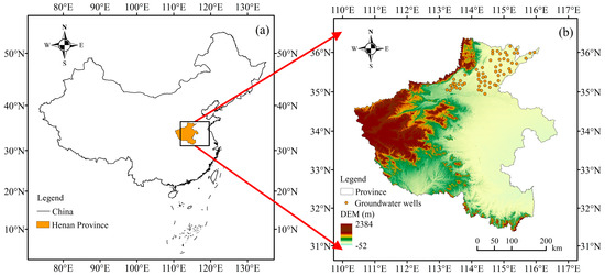
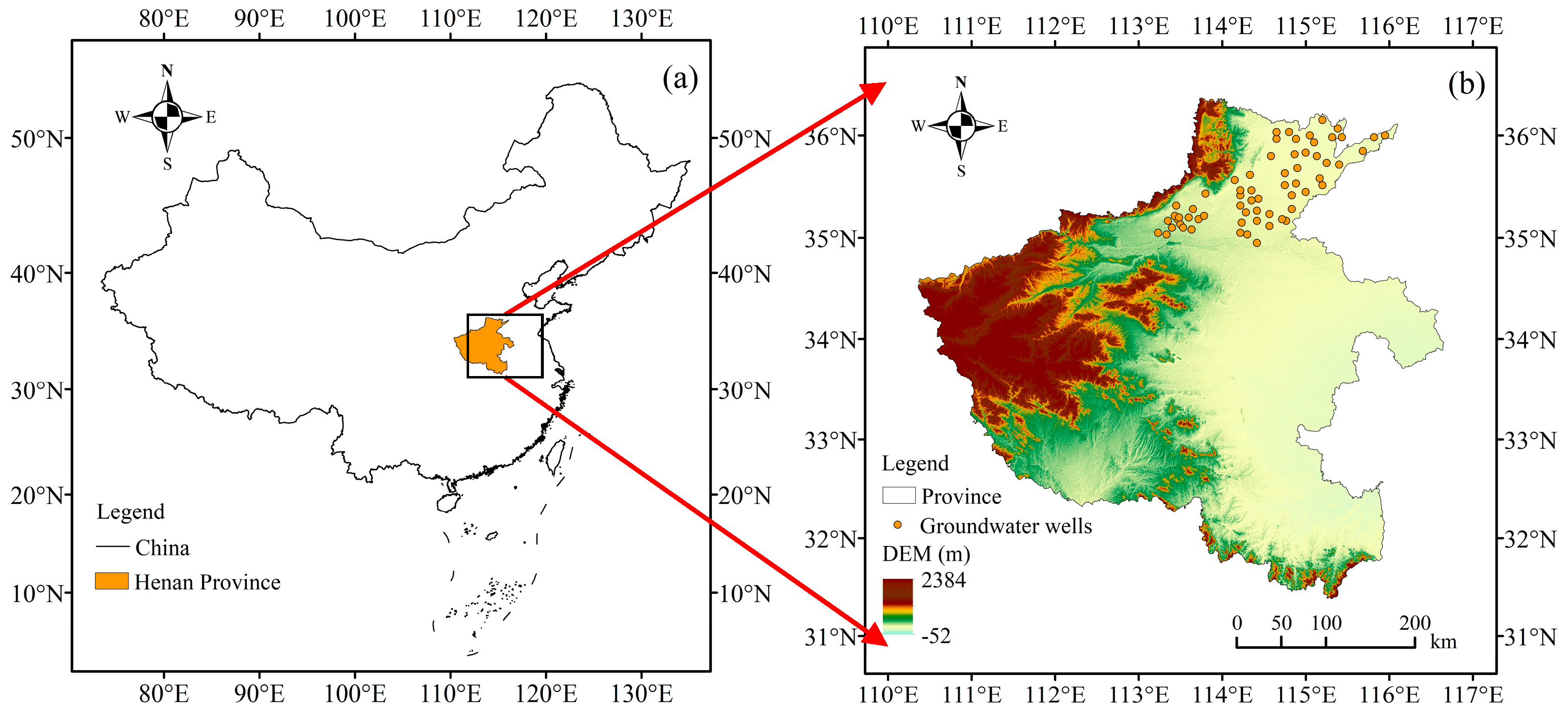
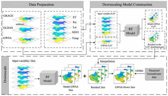
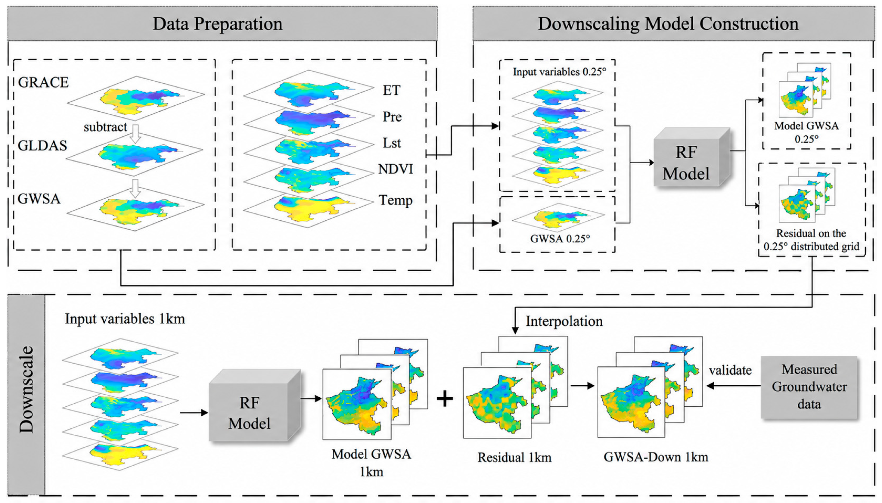
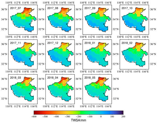
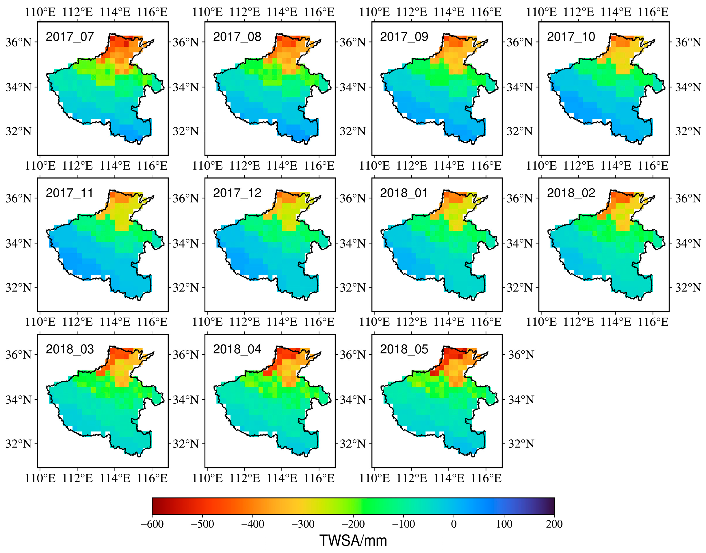
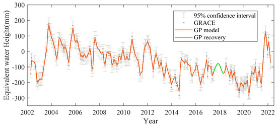
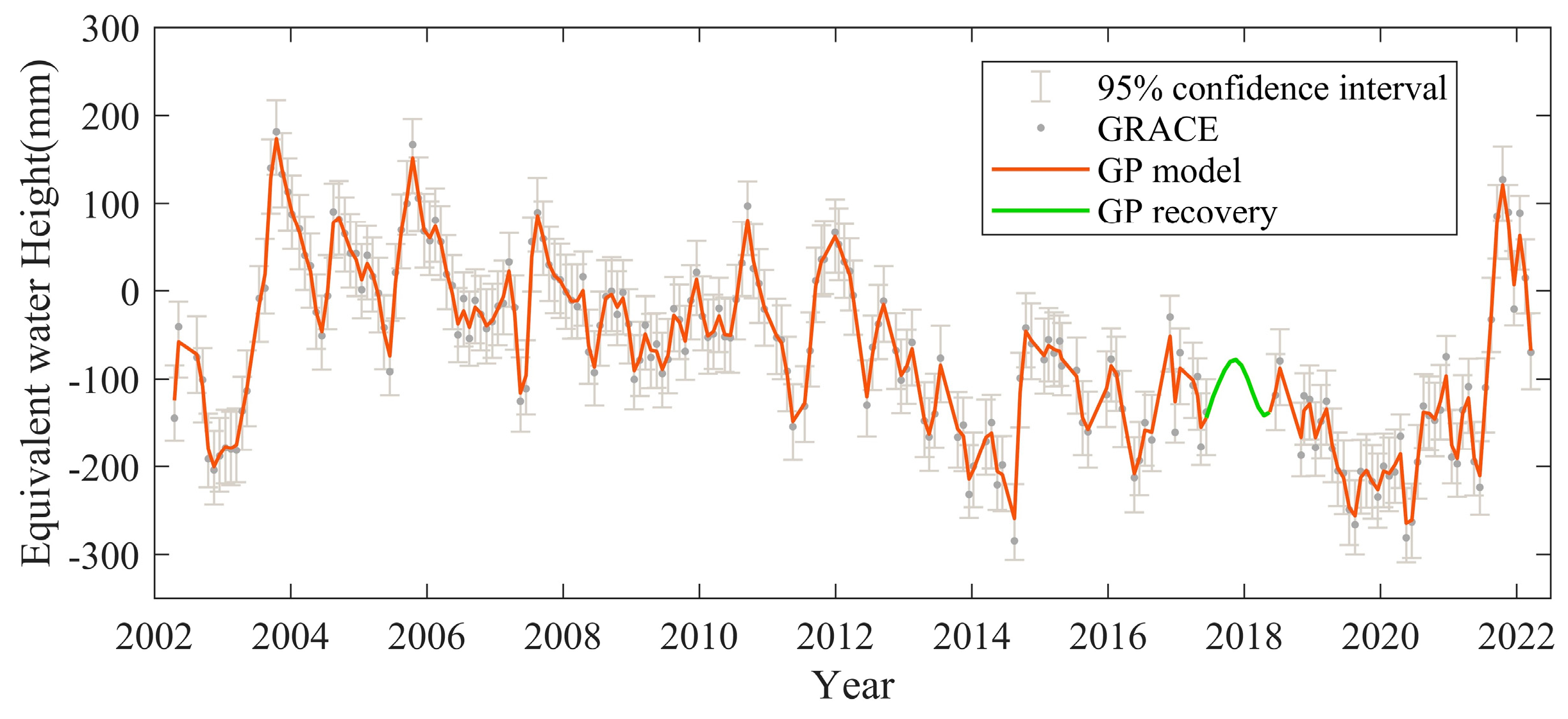
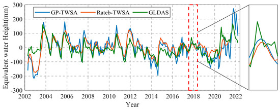
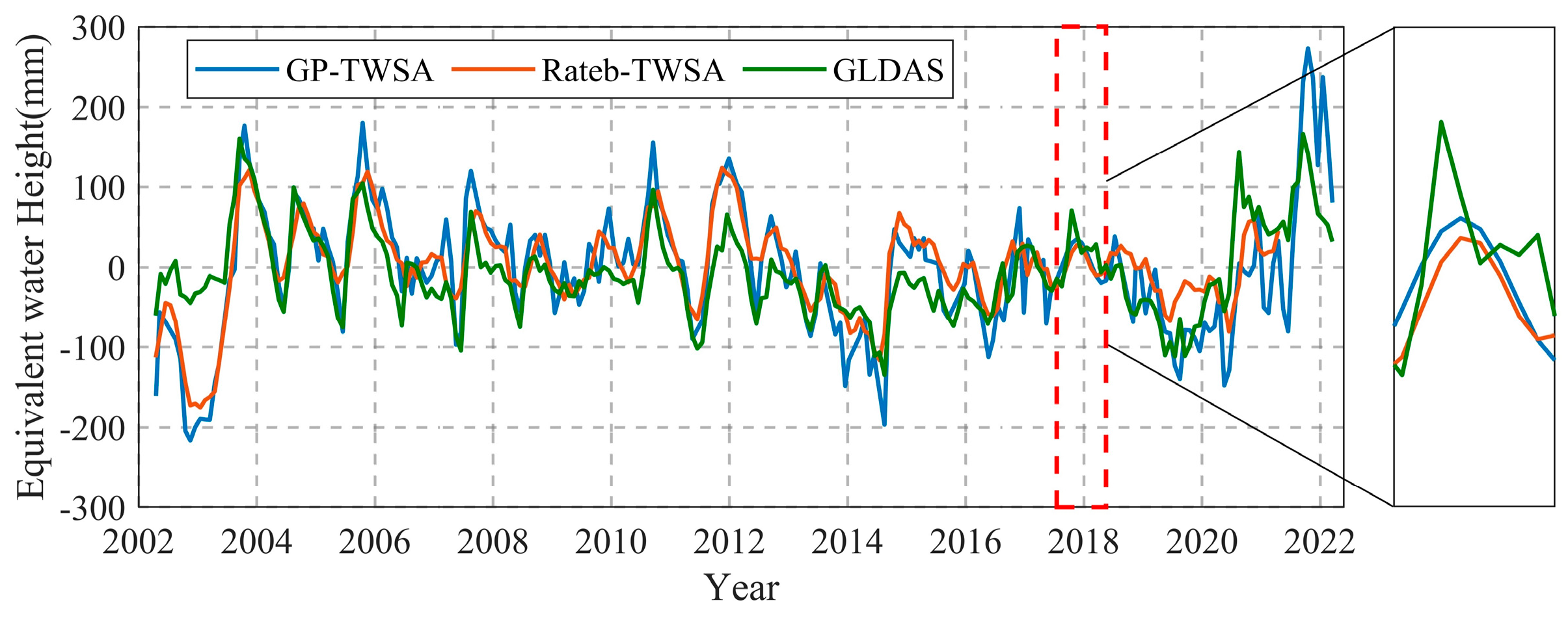
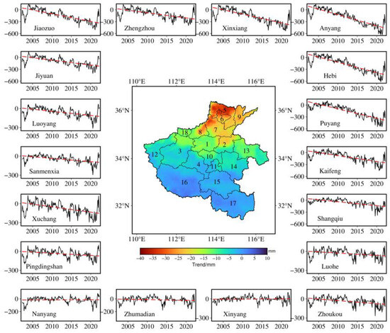
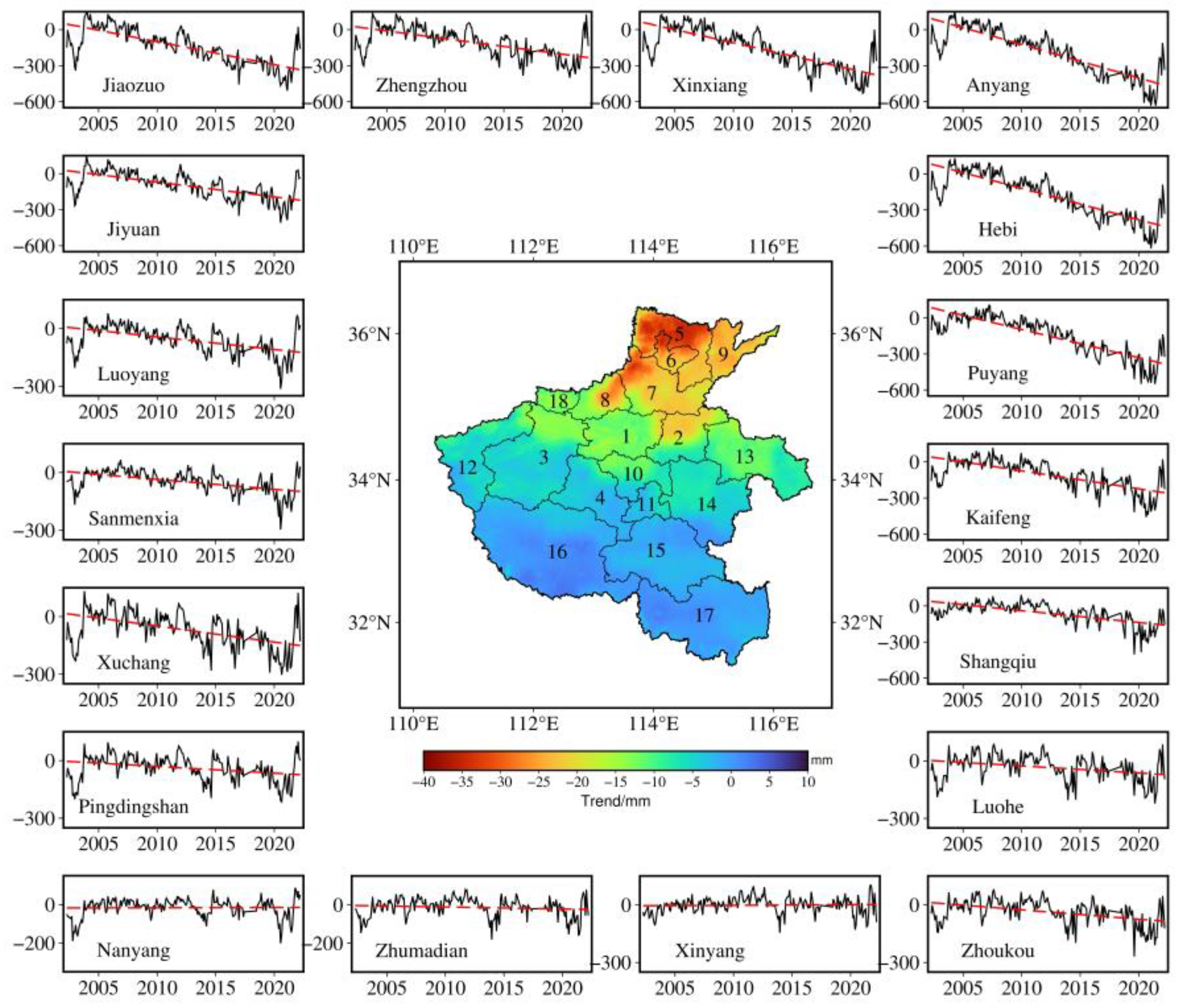
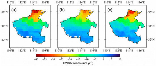
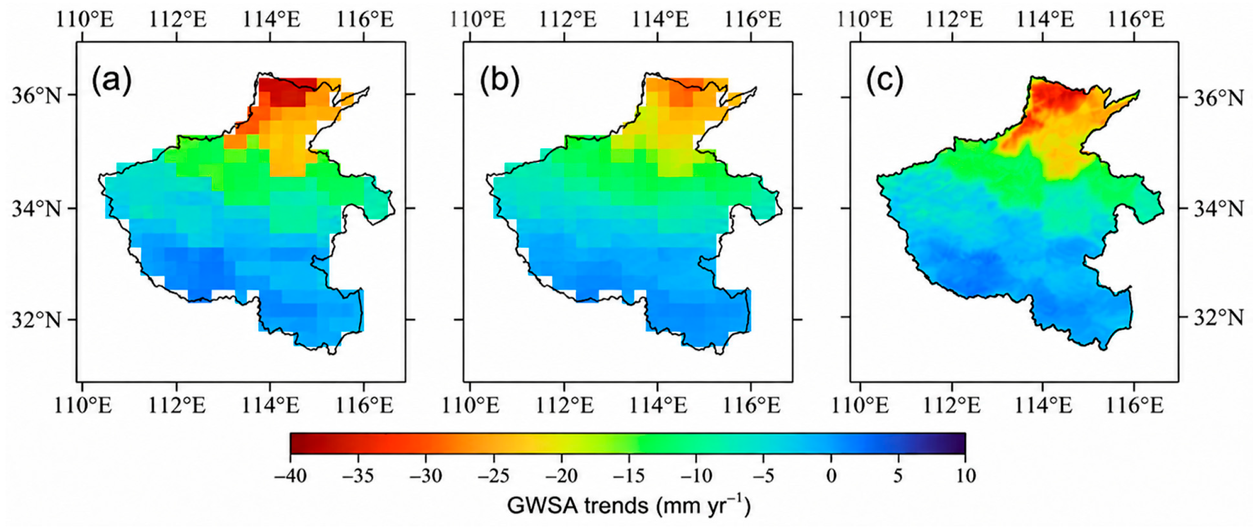
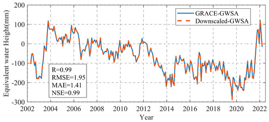
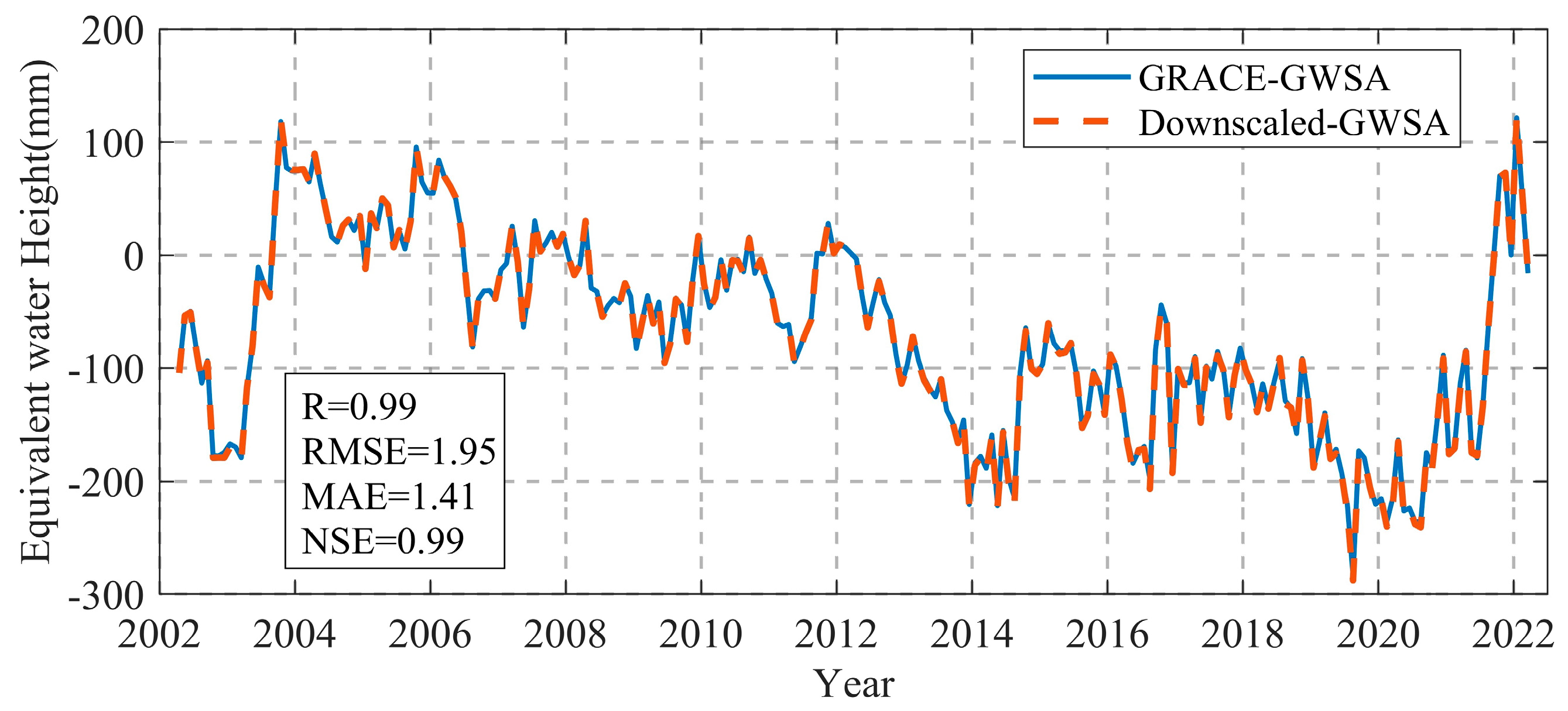
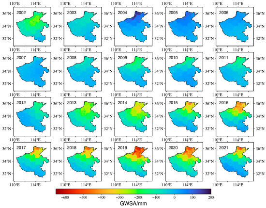
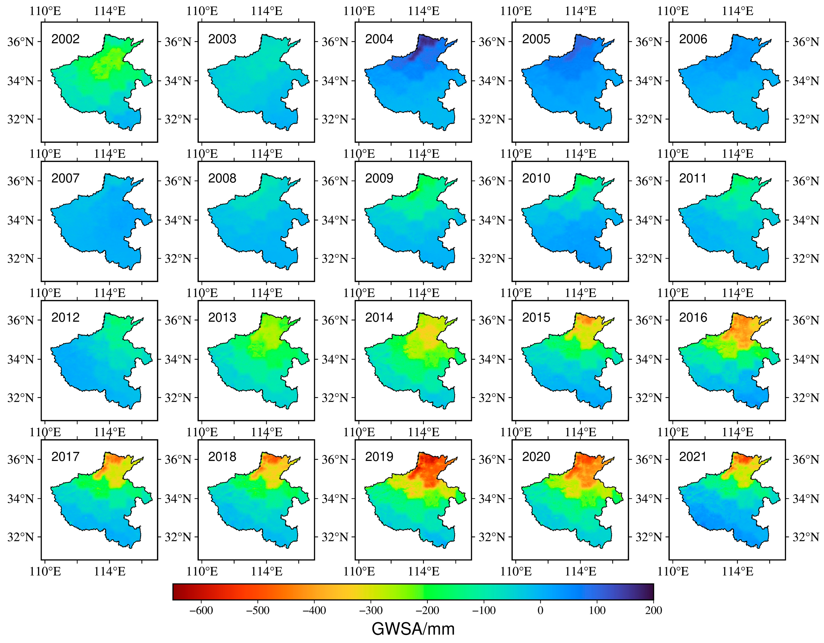
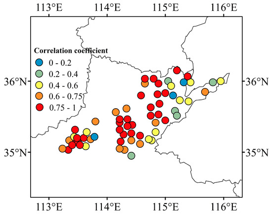
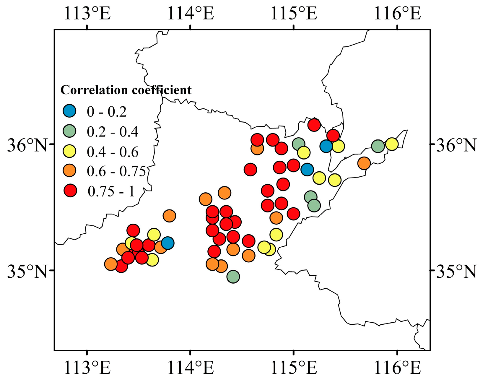
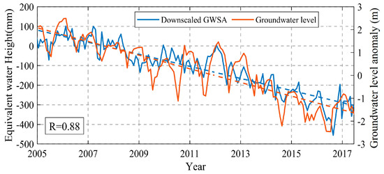
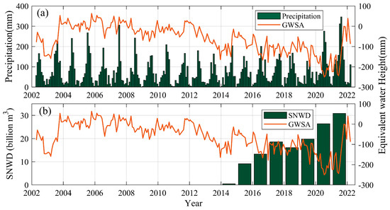
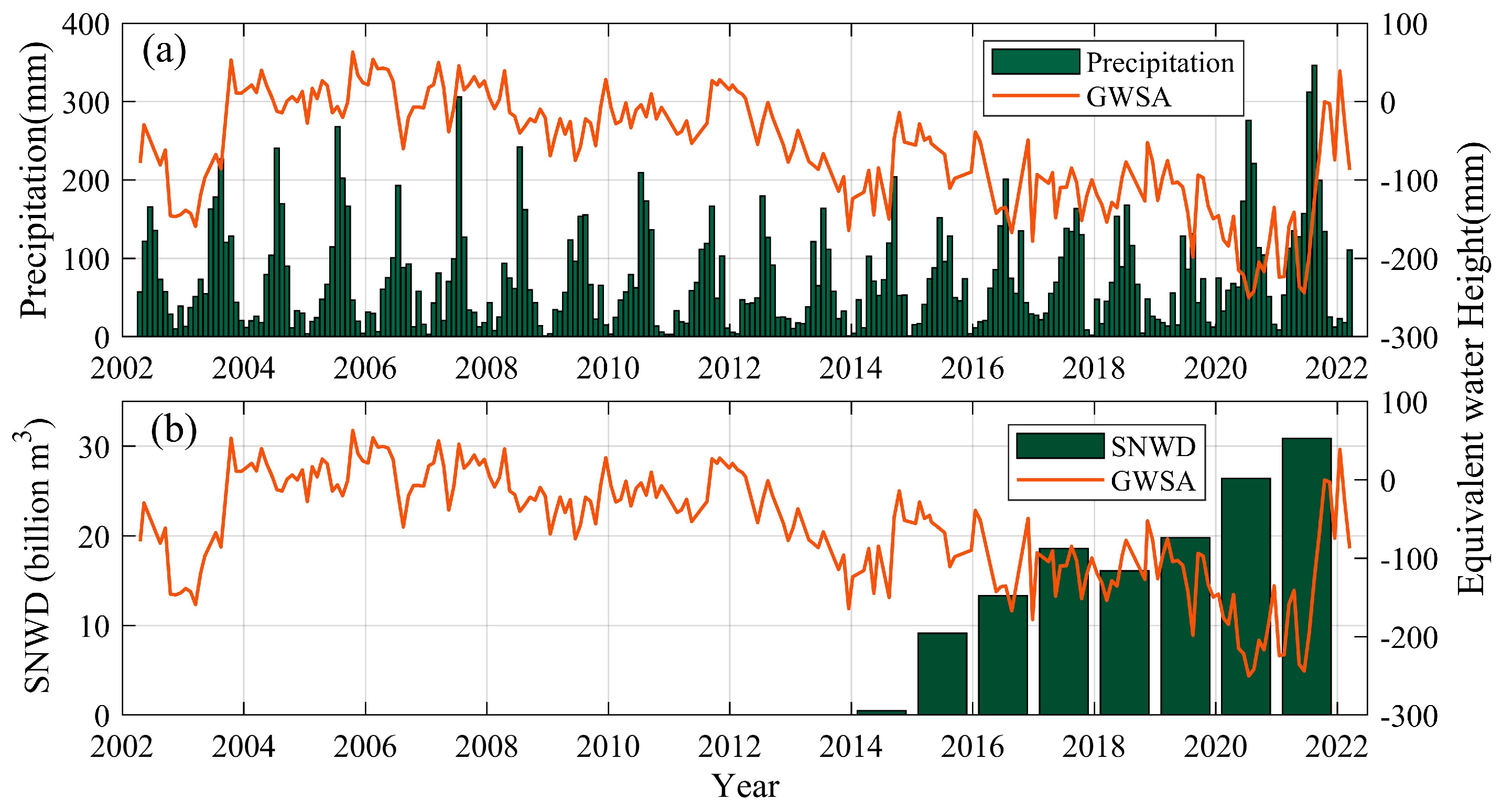
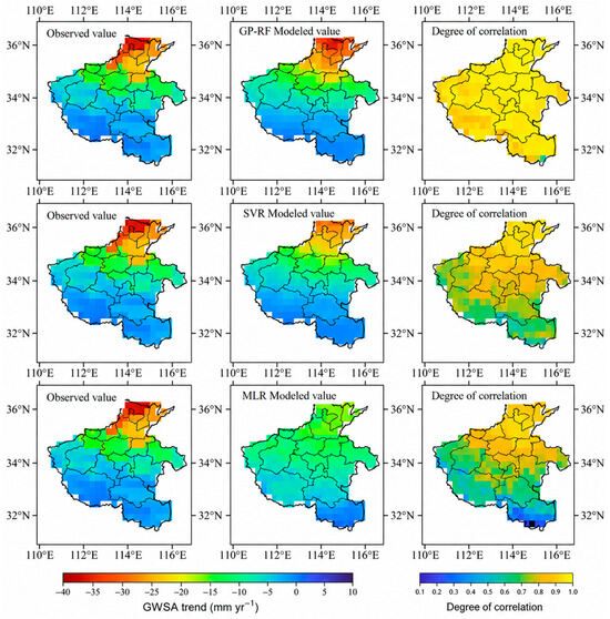
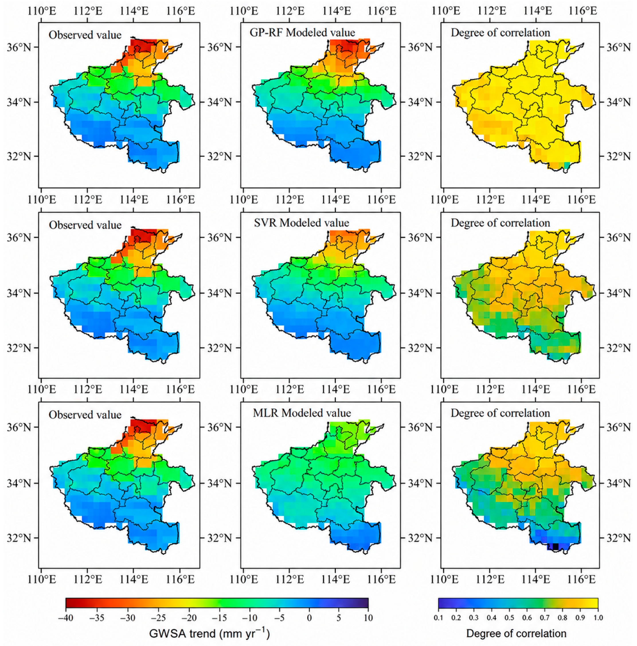

Disclaimer/Publisher’s Note: The statements, opinions and data contained in all publications are solely those of the individual author(s) and contributor(s) and not of MDPI and/or the editor(s). MDPI and/or the editor(s) disclaim responsibility for any injury to people or property resulting from any ideas, methods, instructions or products referred to in the content. |
© 2026 by the authors. Licensee MDPI, Basel, Switzerland. This article is an open access article distributed under the terms and conditions of the Creative Commons Attribution (CC BY) license.