Characterizing the Mismatch Between ECOSTRESS-Derived Land Surface Temperature and ENVI-Met-Simulated UTCI Across Local Climate Zones

Highlights

What are the main findings?

• Across 24 Seoul LCZ plots, the primary near-date relationship between ECOSTRESS LST and ENVI-met-simulated UTCI was weak (R² = 0.040), and the four cross-date sensitivity observations also showed low explanatory power (R² = 0.000–0.126).
• Descriptive LCZ-level mismatch patterns showed that satellite-observed surface thermal conditions did not consistently reproduce model-based pedestrian heat-exposure patterns.

What are the implications of the main findings?

• Under this design, satellite LST did not show stable performance as a screening proxy for simulated pedestrian heat exposure.
• The Conditional Proxy Efficacy (CPE) construct is retained only as a conceptual, hypothesis-generating way to organize observed mismatch patterns.

Abstract

Satellite-derived land surface temperature (LST) is widely used for urban heat assessment, but its correspondence with pedestrian exposure is uncertain. We compared ECOSTRESS-derived LST with ENVI-met-simulated Universal Thermal Climate Index (UTCI), treated as a model-based heat-exposure indicator, across 24 Seoul Local Climate Zone plots. One ECOSTRESS scene acquired five days before the ENVI-met simulation served as the primary near-date, hour-matched comparison under comparable meteorological conditions rather than a simultaneous field observation; four scenes from 2021–2025 were treated as separate cross-date sensitivity observations. A source audit retained 118 of 120 plot × scene records. The primary association was weak (r = 0.199, p = 0.351, R² = 0.040, n = 24). The unadjusted pooled benchmark explained 6.1% of UTCI variance, whereas the scene-adjusted LST slope was 0.060 °C UTCI per °C LST (plot-cluster-robust 95% CI −0.075 to 0.195; p = 0.371). Because only two plots represented each LCZ, leave-one-plot-out and stratified bootstrap results were interpreted only as discrete perturbation diagnostics. ECOSTRESS LST therefore did not demonstrate stable proxy performance for simulated pedestrian heat exposure under this design. CPE is retained as a conceptual organizing heuristic, not a validated classifier or transferable LCZ ranking.

1. Introduction

Global climate change is increasing the frequency and intensity of extreme heat events, leading to rising mortality and disease burdens across regions [1]. Recent global studies further show that anthropogenic climate change has already increased heat-related mortality and that deadly heat exposure is becoming a widespread public-health risk under continued warming [2,3]. In cities, the combined effects of urban heat islands (UHIs), heatwaves, climate background, and population growth make heat risk a major challenge for sustainable urban development [4,5].

Satellite-derived land surface temperature (LST) has become a key data source for urban thermal research. Among available thermal infrared platforms, Landsat Collection 2 Level-2 products have been especially influential because of their long archive and standardized processing. Compared with Landsat, ECOSTRESS provides finer native thermal spatial resolution and variable overpass timing, offering a complementary basis for examining urban thermal heterogeneity at the LCZ scale. Thermal infrared remote sensing enables spatially continuous monitoring of LST, surface urban heat islands (SUHIs), surface characteristics, and energy-related processes across cities [6,7,8]. Macro-scale urban climate studies have therefore widely used LST and SUHI intensity as proxy indicators for comparing urban thermal environments [9,10,11]. However, this proxy-based approach assumes that LST is consistently related to near-surface air temperature and pedestrian-scale thermal conditions. Recent studies challenge this assumption, showing that LST may differ substantially from conditions represented by pedestrian-level biometeorological indicators, especially in complex urban forms and hot–humid climates [12].

Within the LCZ framework, LST is often expected to show a positive relationship with pedestrian heat exposure. Yet emerging evidence indicates that this relationship is not universal. Urban morphology, surface cover, street-canyon geometry, shading, ventilation, and urban fabric may decouple surface radiative temperature from pedestrian-level exposure [12,13,14]. As a result, high LST may not always correspond to high simulated UTCI-based heat exposure, while moderate LST may coincide with elevated simulated UTCI under strong solar exposure or weak ventilation.

Recent studies reinforce the need to treat surface temperature and pedestrian heat exposure as context-dependent but distinct outcomes. An ECOSTRESS analysis of 179 golf courses in the Seoul Metropolitan Area showed that diurnal LST cooling or warming depended on internal landscape configuration and surrounding land-use context [15]. Complementary field-informed ENVI-met studies in Shenyang, Zhenjiang, and Nanjing found that pedestrian-level PET or UTCI varied with building height, street orientation, canyon aspect ratio, vegetation or tree species, and user-group-specific thermal perception [16,17,18]. Together, these findings support morphology-aware interpretation but do not establish direct equivalence between remotely sensed LST and pedestrian thermal exposure.

Briegel et al. [19] already showed that daytime satellite LST can be a poor proxy for intra-urban heat-stress variability and that morphology-aware information may perform better. The present study therefore does not claim novelty for the general proposition that LST is an imperfect heat-stress proxy. Its narrower contribution is a source-audited ECOSTRESS–ENVI-met comparison across Seoul LCZ plots, with a primary near-date scene separated from cross-date sensitivity observations.

This mismatch reflects a representational gap between two-dimensional satellite observations and three-dimensional pedestrian exposure conditions. Satellite LST captures surface radiative conditions, whereas UTCI integrates air temperature, radiation, humidity, and wind at pedestrian height [19]. Microclimate models such as ENVI-met provide a way to examine these processes because they simulate surface–atmosphere interaction, radiation exchange, airflow, and pedestrian-level biometeorological variables at high spatial and temporal resolution [20]. In this study, however, UTCI is derived from simulated inputs and is therefore interpreted as a model-based heat-exposure indicator rather than a directly observed measure of individual thermal sensation or physiological response.

Therefore, the aim is not to reject LST for urban thermal research but to test whether its association with a model-based pedestrian heat-exposure indicator is stable enough to justify screening claims in this limited Seoul sample. By integrating satellite-derived LST, LCZ classification, and ENVI-met outputs, the study addresses three research questions:

(1)

To what extent is satellite-derived LST associated with ENVI-met-simulated UTCI across different LCZ types?

(2)

Which surface, morphological, and simulated microclimatic conditions are associated with divergence between LST and UTCI?

(3)

Which LCZ-level mismatch patterns recur descriptively, and which patterns remain too uncertain for interpretation without larger samples and direct field validation?

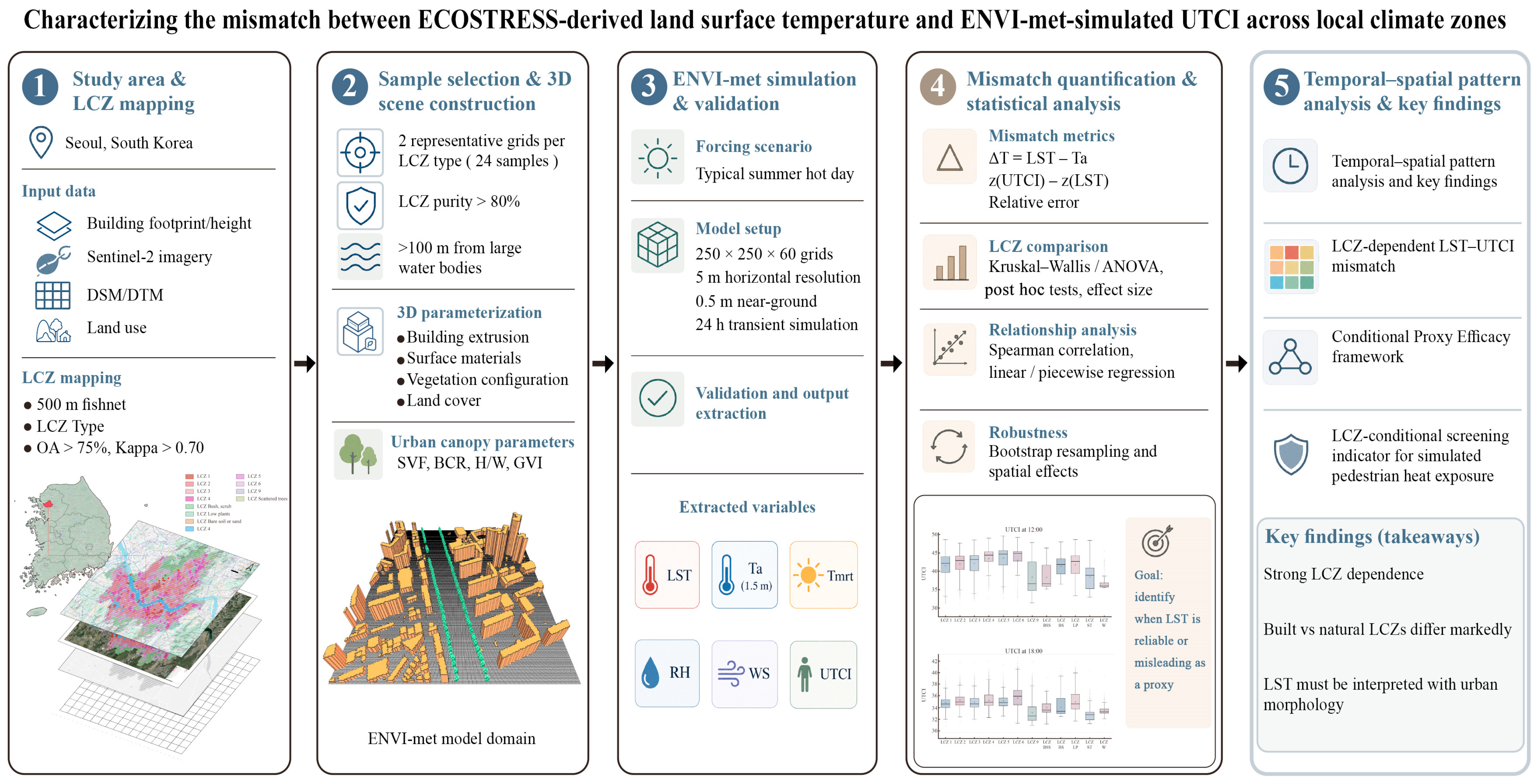
By answering these questions, the study seeks to clarify the applicability boundaries of remote-sensing-based heat assessment and to provide an LCZ-sensitive descriptive synthesis rather than a validated proxy framework. The overall study workflow is summarized in Figure 1.

2. Materials and Methods

2.1. Study Area and Sampling

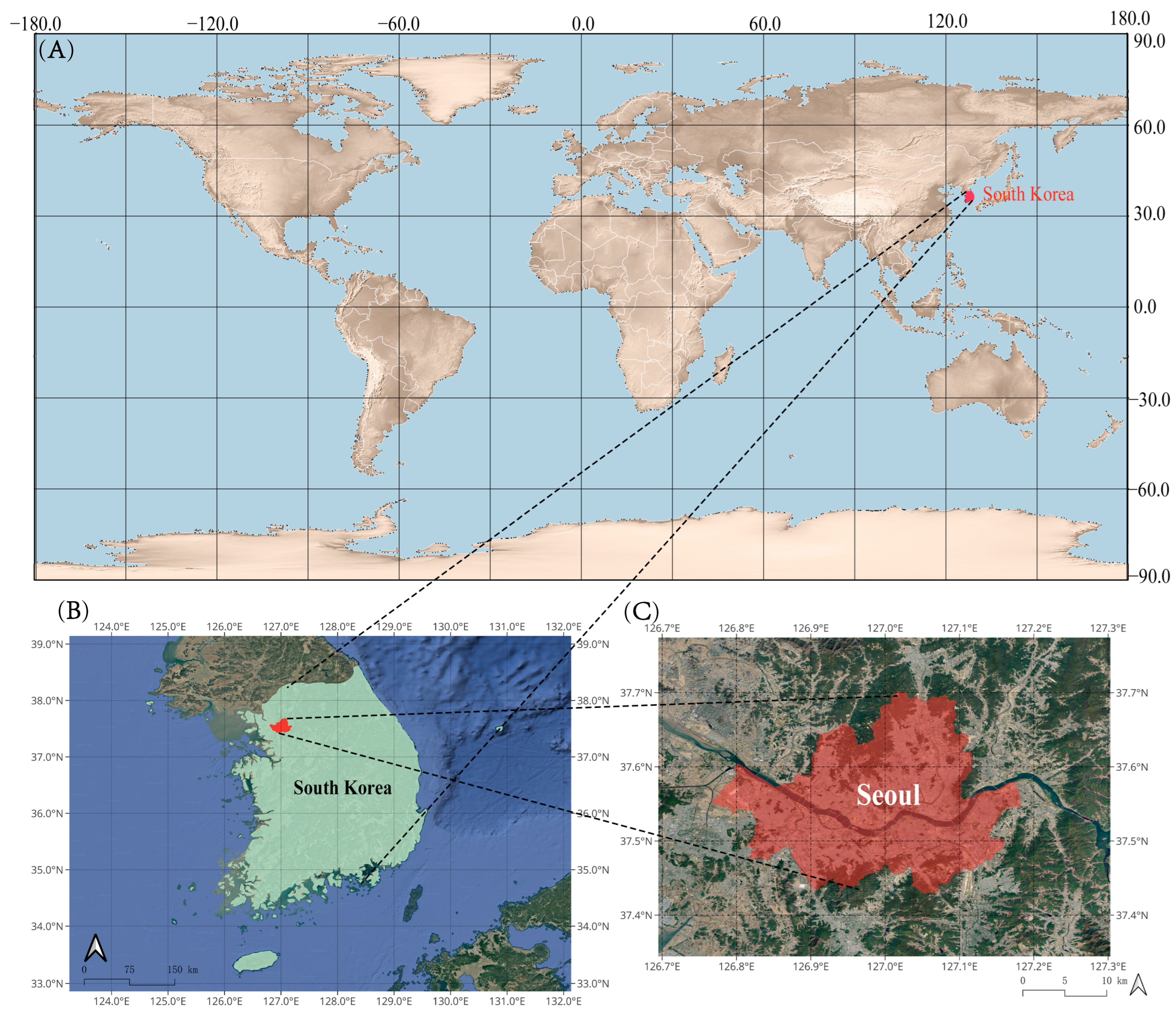
Seoul (37°34′N, 126°59′E) provides an ideal experimental setting for examining thermal heterogeneity across local climate zones (LCZs). The city is located in the Han River basin in the central Korean Peninsula and has a temperate monsoon climate characterized by hot and humid summers and cold, dry winters [21]. As of 2023, Seoul has a resident population of approximately 9.4 million, with an average population density of 16,000 persons/km², forming a typical high-density East Asian urban structure characterized by a “dense core–open periphery” pattern [22]. The geographic location of Seoul is shown in Figure 2.

Notably, Seoul exhibits a pronounced urban heat island (UHI) effect. Long-term meteorological observations indicate that the temperature difference between the urban core and surrounding suburban areas can reach 3.5–4.8 °C in autumn, with nighttime peak intensity up to 4.3 °C [23]. Recent studies further show that surface temperature differences among LCZ types can exceed 6 °C during heatwave events [24]. This strong urban thermal gradient, combined with the diversity of LCZ types—dominated by compact mid-rise (LCZ 2, 23.6% of built-up areas) and supplemented by open low-rise (LCZ 6, 4.0%) [21]—provides a useful context for examining the mismatch between LCZ characteristics and simulated pedestrian heat exposure.

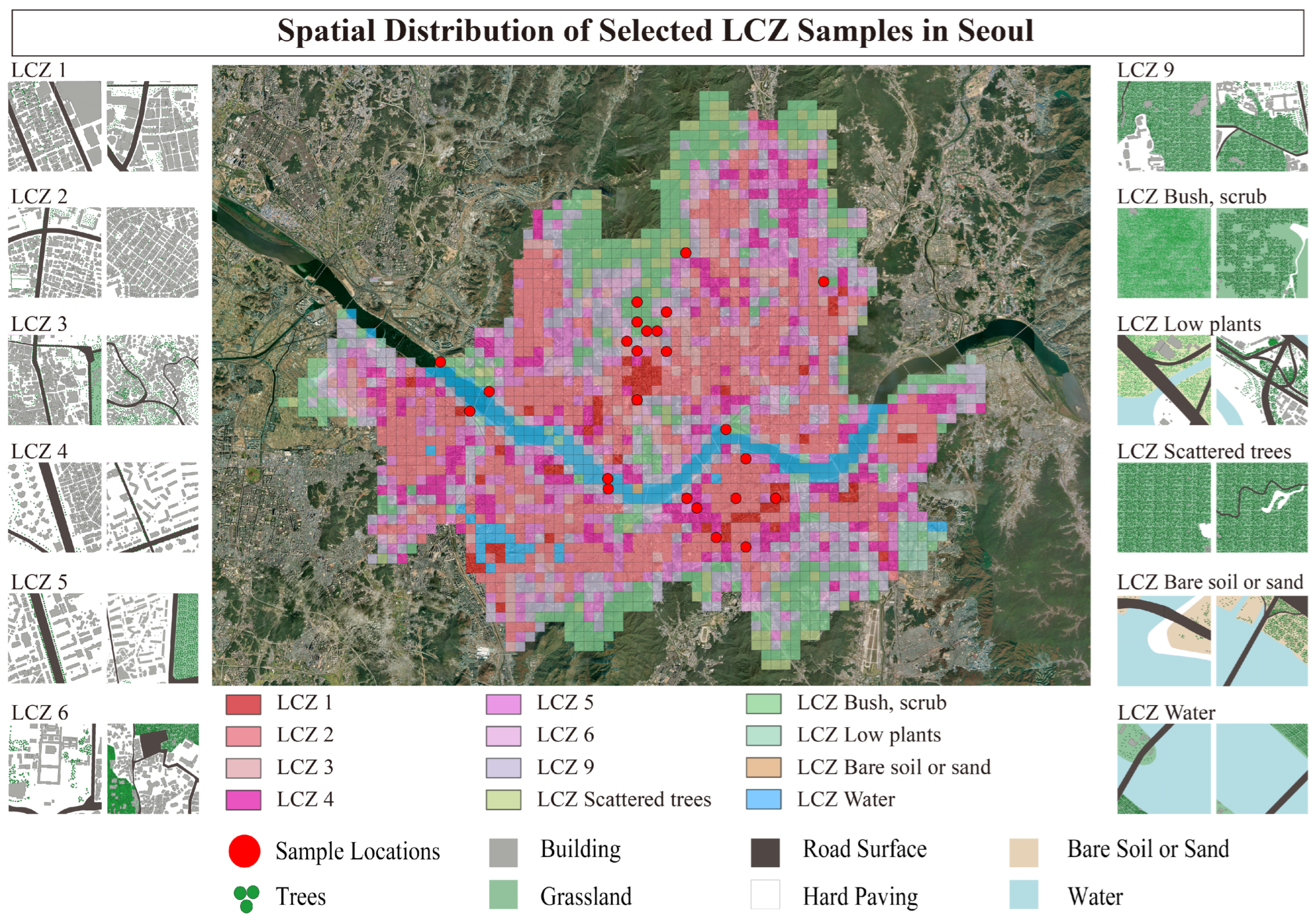
LCZs provide a standardized urban-climate typology based on surface cover, urban structure, construction materials, and human activity [25,26]. The selected built classes were LCZ 1, 2, 3, 4, 5, 6, and 9, and the selected land-cover classes were the Stewart–Oke classes B, C, D, F, and G. For compact figure and table labels, this study used the study-specific aliases LCZ-ST, LCZ-BS, LCZ-LP, LCZ-BSS, and LCZ-W, respectively. These aliases are not additional canonical LCZ classes. The study area was divided into 500 m × 500 m plot units, consistent with the local-scale range discussed for LCZ thermal source areas [26,27]. The sample distribution is shown in Figure 3.

LCZ mapping was conducted following the WUDAPT Level 0 protocol and was further refined using GIS-assisted multi-source remote-sensing analysis. Sentinel-2 multispectral imagery, building footprint data, and digital surface model (DSM) data were integrated to derive land-cover and urban canopy indicators relevant to LCZ classification. A Random Forest classifier was trained using manually labeled LCZ training areas, and the preliminary classification was iteratively checked through high-resolution imagery and urban morphology data. To assess classification reliability, an independent validation sample was used to generate a confusion matrix. Overall accuracy, the kappa coefficient, and class-specific producer’s and user’s accuracies were calculated. The final LCZ map achieved an overall accuracy of 84.6% and a kappa coefficient of 0.81, with class-specific F1 scores ranging from 0.71 to 0.93. Classes with lower classification confidence were manually reviewed and, where necessary, excluded from the selection of representative plots. This quality-control procedure was used to reduce the risk that subsequent LST–UTCI comparisons were affected by LCZ misclassification [25,28].

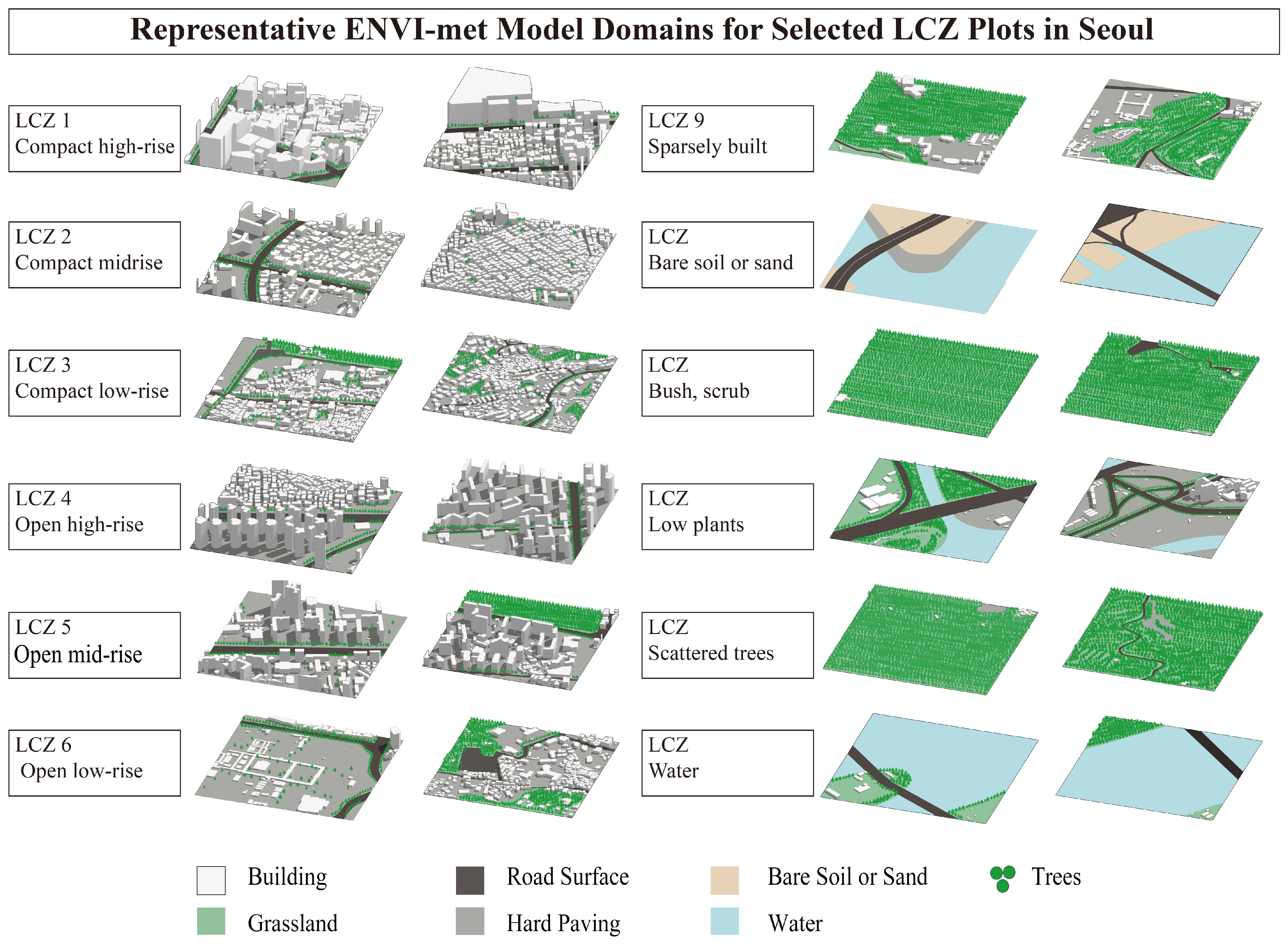
Within each LCZ type, two representative 500 m × 500 m plots were selected, resulting in 24 plots. The plot—not an individual raster cell—was the independent sampling unit. Valid ECOSTRESS pixels and valid ENVI-met cells were summarized separately within the same plot polygon and then paired by plot and scene; ECOSTRESS was not upsampled to create independent 5 m observations. Grid-/cell-level maps and distributions were retained only for descriptive visualization. The representative ENVI-met domains are illustrated in Figure 4.

This stratified sampling strategy balanced LCZ-level representativeness and within-plot observational density, enabling comparisons of LST, air temperature, and UTCI to reflect systematic differences in urban form, surface cover, and land-use function [29,30,31].

Representative plots were selected using LCZ-specific criteria. For built LCZs, three criteria were applied: (1) LCZ purity greater than 80% within the 500 m × 500 m plot [25,26]; (2) a distance greater than 100 m from large water bodies, except where the influence of water was part of the target LCZ context [32,33]; and (3) predominantly residential or commercial land use, in order to reduce variability caused by industrial anthropogenic heat sources [21]. For natural and land-cover LCZs, including LCZ B, LCZ C, LCZ D, LCZ F, and LCZ G, the selection criteria were modified to prioritize surface-cover homogeneity, spatial continuity, and consistency with the standard LCZ definition. LCZ G plots were selected to represent water-dominated environments and were therefore not subject to the water-distance exclusion criterion.

2.2. Variables and Data

Table 1. Summary of input data and analytical variables.

Study Area	Seoul, Republic of Korea
Geographic coordinates	37.5665°N, 126.9780°E
Simulation date	30 July 2025
Simulation period	24-h run; 00:00 30 July to 00:00 31 July 2025 (25 hourly endpoints)
Temporal resolution of ENVI-met outputs	1 h
Satellite reference	ECOSTRESS Collection 2 L2T LSTE Version 002 (ECO_L2T_LSTE.002)
ECOSTRESS native spatial resolution	70 m
ENVI-met horizontal grid resolution	5 m × 5 m
Vertical extraction height for pedestrian-level variables	1.5 m
Aggregation unit	500 m × 500 m LCZ plot
Primary simulated heat-exposure indicator	ENVI-met-simulated Universal Thermal Climate Index (UTCI)

summarizes the key datasets, spatial and temporal settings, and analytical variables used in this study. ECOSTRESS Collection 2 L2T LSTE Version 002 data provided native 70 m satellite-derived LST, while ENVI-met simulations provided hourly 5 m × 5 m microclimate outputs. Pedestrian-level variables were extracted at 1.5 m, and the 500 m × 500 m LCZ plot was used as the main aggregation unit.

2.2.1. Satellite-Derived Land Surface Temperature

Satellite-derived LST was obtained from the ECOSTRESS Collection 2 Tiled LST and Emissivity Level-2 product (ECO_L2T_LSTE.002) at 70 m native resolution [34,35,36]. Five daytime granules for tile 52SCG were converted from Kelvin to degrees Celsius and matched to the nominal ENVI-met outputs using their actual acquisition times (

Table 2. Metadata and temporal matching of the ECOSTRESS Collection 2 L2T LSTE granules used in the satellite–model comparison.

Nominal Output	ECOSTRESS Producer Granule ID	Acquisition Interval	Date Offset/Role
10:00	ECOv002_L2T_LSTE_ 39212_008_52SCG_ 20250606T011853_0713_01	6 June 2025 UTC 01:18:53–01:19:45 KST 10:18:53–10:19:45	54 d Sensitivity
12:00	ECOv002_L2T_LSTE_ 28151_018_52SCG_ 20230624T022820_0711_01	24 June 2023 UTC 02:28:20–02:29:12 KST 11:28:20–11:29:12	767 d Sensitivity
14:00	ECOv002_L2T_LSTE_ 39979_005_52SCG_ 20250725T054637_0713_01	25 July 2025 UTC 05:46:37–05:47:29 KST 14:46:37–14:47:29	5 d Primary near-date
16:00	ECOv002_L2T_LSTE_ 17315_013_52SCG_ 20210726T074707_0712_01	26 July 2021 UTC 07:47:07–07:47:59 KST 16:47:07–16:47:59	1465 d Sensitivity
18:00	ECOv002_L2T_LSTE_ 17550_017_52SCG_ 20210810T085516_0712_01	10 August 2021 UTC 08:55:16–08:56:07 KST 17:55:16–17:56:07	1450 d Sensitivity

Note: All granules are daytime observations from tile 52SCG and belong to ECO_L2T_LSTE.002. Clock-time offsets, calculated from scene midpoints, were approximately +19, −31, +47, +48, and −4 min relative to the nominal ENVI-met outputs. The five scenes do not constitute a same-day satellite diurnal cycle.

).

Processing retained cloud-free pixels with valid LST, emissivity, LST uncertainty, and mandatory/input-data quality flags; water was retained only for LCZ-W. For inferential analyses, valid 70 m ECOSTRESS pixels were summarized within each 500 m plot and paired with the corresponding plot-level summary of valid 5 m ENVI-met cells. There was no one-to-one 70 m-to-5 m pixel matching or artificial replication. Full QC-bit logic, valid-pixel counts, LST_err summaries, and the inclusive-mask sensitivity are reported in Supplementary Method S1.

2.2.2. ENVI-Met Simulated Surface Temperature and Microclimate Variables

ENVI-met simulations were conducted using ENVI-met version 5.6.1. ENVI-met-simulated surface temperature was used as the model-based counterpart of satellite-derived LST. ENVI-met simulates urban surface–atmosphere interactions, radiation exchange, airflow, vegetation processes, and energy balance at high spatial and temporal resolution, and has been widely used in model-based pedestrian heat-exposure and outdoor thermal-comfort studies [20,37,38].

To avoid conceptual ambiguity, two surface-temperature variables were distinguished. LST_sat refers to satellite-derived land surface temperature, while LSTsim refers to ENVI-met-simulated surface temperature. In addition to LSTsim, ENVI-met outputs included air temperature, relative humidity, wind speed, and mean radiant temperature at pedestrian height. These variables were extracted hourly and used to calculate UTCI [20,37,39].

2.2.3. Model-Based Heat-Exposure Indicator: UTCI and Air Temperature

Air temperature refers to ENVI-met-simulated air temperature at 1.5 m above ground level, corresponding to pedestrian breathing height. Outdoor heat exposure is not determined by air temperature alone, but is also influenced by humidity, wind speed, and the radiative environment. In this study, the Universal Thermal Climate Index (UTCI) was calculated entirely from ENVI-met outputs and is therefore treated as a simulated, model-based indicator of pedestrian heat exposure. It is not interpreted as a directly observed measure of individual thermal sensation, physiological response, or health outcome.

Hourly UTCI values at pedestrian height were calculated using the BioMet module of ENVI-met. The UTCI-Fiala framework integrates air temperature, mean radiant temperature, wind speed, and water vapor pressure to represent thermophysiological heat-load conditions [40,41]. Because these meteorological inputs were simulated, the resulting UTCI values were used for relative comparison among LCZs and not as independently field-validated observations of human heat stress.

The operational UTCI approximation can be expressed as

UTCI = Ta + Offset(Ta, Tmrt, va, pa)

where Ta is air temperature, Tmrt is mean radiant temperature, va is wind speed, and pa is water vapor pressure. The offset term represents the deviation between the outdoor environment and the UTCI reference environment. In this study, all four inputs were obtained from hourly ENVI-met outputs at pedestrian height [40]; consequently, the derived UTCI is referred to throughout as simulated UTCI or a simulated heat-exposure indicator.

Table 3. Classification of UTCI thermal stress (adapted from Bröde et al., 2012) [40].

UTCI (°C)	Grade of Physiological Stress
<−40	extreme cold stress
−40~−27	very strong cold stress
−27~−13	strong cold stress
−13~0	moderate cold stress
0~9	slight cold stress
9~26	no thermal stress
26~32	moderate heat stress
32~38	strong heat stress
38~46	very strong heat stress
>46	extreme heat stress

presents the UTCI thermal-stress categories used to describe the simulated pedestrian heat-exposure conditions. The UTCI scale combines air temperature, radiation, humidity, and wind into standardized thermophysiological categories. In this study, these categories were used to compare modeled exposure conditions across LCZ types. They should not be read as direct observations of individual physiological stress, subjective thermal sensation, or health effects.

2.2.4. Temporal Setting and Data Extraction

The ENVI-met run covered 24 h from 00:00 on 30 July to 00:00 on 31 July 2025. Including both endpoints yielded 25 hourly timestamps. Main diurnal displays use 00:00–23:00, whereas the endpoint was retained for validation matching where both observed and modeled values were complete.

Each ECOSTRESS acquisition was assigned to the nearest of the five preselected ENVI-met comparison outputs (10:00, 12:00, 14:00, 16:00, and 18:00 KST) according to its actual local acquisition time. These nominal comparison bins were retained for consistency with the predefined analysis schedule. The midpoint clock-time offsets were approximately +19, −31, +47, +48, and −4 min, respectively. Linear interpolation was not used.

For the LCZ-level three-time descriptive summary, valid ENVI-met grid cells at 10:00, 14:00, and 18:00 were first summarized using the spatial median within each representative plot, with −999 no-data values excluded. The LCZ-level value was then calculated as the median of the Plot 1 and Plot 2 spatial medians.

Because the five scenes were acquired on different dates and years, they were treated as separate cross-date, local-time-matched spatial observations rather than a same-day or pseudo-diurnal satellite sequence. The 25 July 2025 scene, acquired five days before the simulation, was designated as the primary near-date comparison; the remaining four scenes were used as supplementary cross-date sensitivity observations.

2.2.5. Reference-Station Meteorological Context for the ECOSTRESS Scenes

City-scale meteorological context was obtained from Seoul ASOS 108 (WMO 47108; ISD 471080-99999) [42]. Air temperature, dew point, and wind speed were linearly interpolated to each ECOSTRESS acquisition time, relative humidity was calculated from air and dew-point temperature, and the nearest valid total-cloud-cover observation was retained. The matched overpass conditions and daily backgrounds are reported in Table S1a,b; these station values describe macroscale scene context rather than plot-level LCZ conditions.

2.2.6. Partial ENVI-Met Validation Using Air Temperature and Relative Humidity

Field validation was conducted using 10 Spectrum WatchDog 2550 portable weather stations (Spectrum Technologies, Inc., Aurora, IL, USA) deployed at representative LCZ sites in Seoul. Each station recorded air temperature and relative humidity at 1 min intervals and was mounted at 1.5 m above ground level. Observations collected during July 2025 were aggregated to hourly means to match the ENVI-met output resolution, and anomalous or missing records were excluded.

For each validation site, ENVI-met hourly outputs were extracted at the corresponding location and 1.5 m height. The 24 h run produced 25 possible hourly timestamps when both endpoints were counted. After matching and quality control, nine sites retained 25 pairs, and one site retained 24, giving 249 pairs. LCZ-W and LCZ-BSS had no field stations; their ENVI-met fields are therefore model-only. In addition, LCZ-BSS LSTsim values at 10:00, 14:00, and 18:00 (20.2, 20.7, and 20.6 °C, respectively) were unusually close to water and 9–11 °C below simulated air temperature. This physically unusual result is retained as a flagged descriptive case and is not used to support proxy-efficacy or mechanistic claims. Model performance was summarized using RMSE, MAE, MBE, and R².

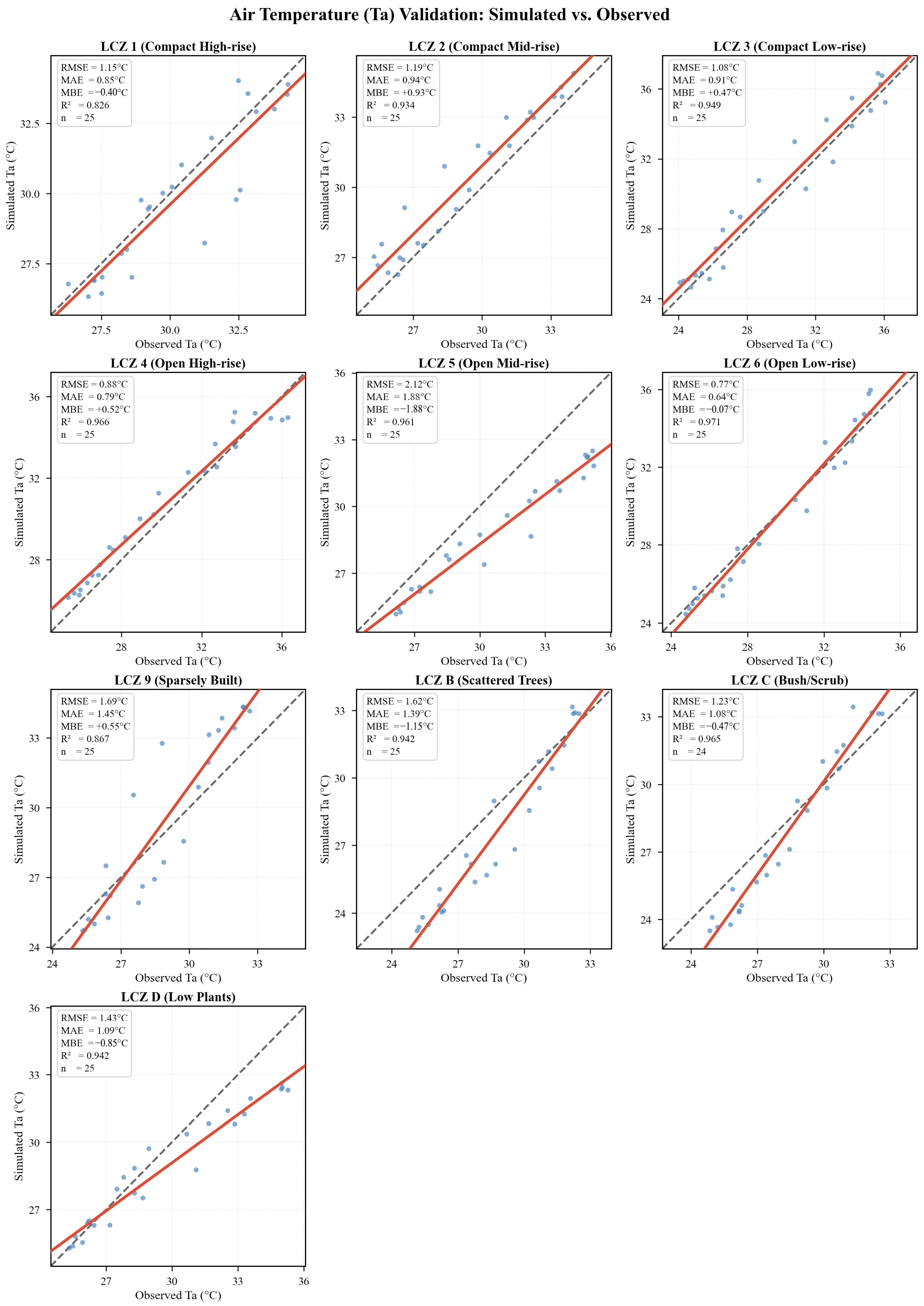
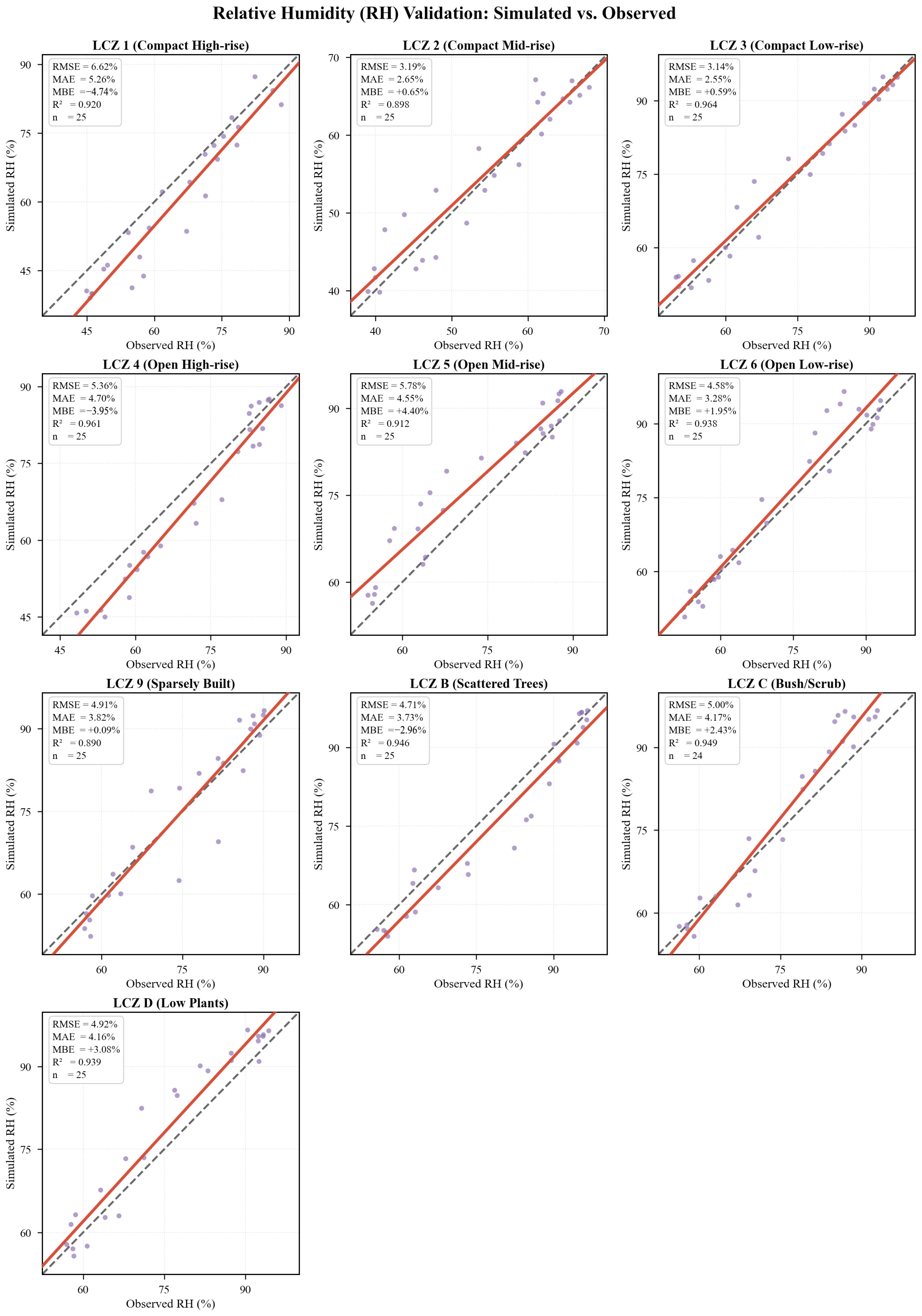
Across the 249 matched hourly pairs, the pooled fit diagnostics were RMSE = 1.37 °C, MAE = 1.10 °C, MBE = −0.23 °C, and R² = 0.850 for air temperature, and RMSE = 4.92%, MAE = 3.89%, MBE = +0.14%, and R² = 0.914 for relative humidity. These pooled R² values combine sites and the shared diurnal cycle and are not independent predictive-validation statistics. Site-specific metrics and sample sizes are shown in Figure 5 and Figure 6.

These matched-period diagnostics show that modeled Ta and RH followed much of the observed temporal variation, but no independent calibration/validation period was available. Pooled agreement can also be inflated by the common diurnal cycle. The diagnostics do not validate UTCI because mean radiant temperature, wind speed, globe temperature, and short- and long-wave radiation were not field validated. All UTCI results are therefore relative, model-based comparisons subject to compound simulation uncertainty.

The field campaign was designed for distributed Ta and RH monitoring at 10 sites. It did not include the synchronized calibrated globe/radiation and three-dimensional wind measurements required for spatially representative MRT and wind validation across the 24 analysis plots; field-derived UTCI could therefore not be calculated. All UTCI analyses remain relative and model-based.

2.3. Mismatch Quantification

2.3.1. Surface–Air Temperature Difference

To quantify the difference between surface thermal conditions and pedestrian-level air temperature, the absolute surface–air temperature difference was calculated as

ΔT_LST-Ta = |LST − Ta|

where LST denotes land surface temperature, and Ta denotes air temperature at 1.5 m above ground. Depending on the comparison, LST denotes either ENVI-met-simulated land surface temperature (LSTsim) or ECOSTRESS-derived land surface temperature (LST_sat).

This metric was used to quantify the decoupling between surface radiative heating and pedestrian-level air thermal conditions. Larger values indicate weaker correspondence between surface temperature and near-surface thermal exposure [12,29,39].

2.3.2. Bias Between Satellite-Derived and ENVI-Met Simulated LST

To evaluate consistency between satellite-observed and model-simulated surface temperature, the signed bias between LSTsim and LST_sat was calculated as

Bias_LST = LSTsim − LST_sat

where LSTsim is ENVI-met-simulated land surface temperature, and LST_sat is ECOSTRESS-derived land surface temperature. Positive values indicate that LSTsim is higher than LST_sat, whereas negative values indicate that LST_sat is higher than LSTsim.

The use of signed bias follows common model-evaluation practice, in which the difference between model outputs and reference observations is used to identify systematic overestimation or underestimation [43]. In this study, the bias metric was calculated across LCZ types and nominal local-time matches to examine whether the discrepancy between satellite-observed and model-simulated surface temperature varied with urban morphology, surface cover, and observational context.

2.3.3. Standardized Mismatch Between LST and UTCI

Because LST and UTCI represent different physical quantities, a standardized mismatch index was constructed using z-score anomalies. LST represents surface radiative temperature, whereas UTCI represents physiological thermal stress determined by air temperature, humidity, wind speed, and radiation.

For each scene, z-score standardization was performed across the QA-valid plot-level LST_sat and plot-level simulated UTCI summaries. The two variables were standardized separately as:

$$z\left(LS{T}_{\mathrm{sat}}\right)={\displaystyle \frac{LS{T}_{\mathrm{sat}}-\overline{LS{T}_{\mathrm{sat}}}}{SD\left(LS{T}_{\mathrm{sat}}\right)}}$$

$$z\left(UTCI\right)={\displaystyle \frac{UTCI-\overline{UTCI}}{SD\left(UTCI\right)}}$$

The standardized mismatch index was then defined as:

Mismatch_LST-UTCI = z(UTCI) − z(LST_sat)

Positive mismatch values indicate that pedestrian-level thermal stress is higher than would be inferred from the satellite-observed LST anomaly alone, implying potential underestimation of human heat exposure by LST. Negative mismatch values indicate that the LST anomaly is higher than the corresponding UTCI anomaly, implying potential overestimation of pedestrian-level thermal stress by LST.

The mismatch index was calculated for each QA-valid plot and summarized within each LCZ using the median and the spread of the two available plot values. With only two plots per LCZ, that spread is a descriptive between-plot quantity, not an estimate of population-level within-LCZ heterogeneity. Each ECOSTRESS scene was assigned to the nearest preselected ENVI-met output by local time; variation among the five matches was treated as cross-date sensitivity, not a same-day trajectory [31].

2.3.4. Intra-Plot Thermal Heterogeneity

To characterize the internal heterogeneity of surface thermal conditions within each 500 m × 500 m LCZ plot, the standard deviation and coefficient of variation of grid-level LST were calculated as

$$\mathrm{CV}={\displaystyle \frac{SD}{\overline{LST}}}\times 100\%$$

where SD is the standard deviation of LST values within a plot, and $\overline{LST}$ is the plot-level mean LST. The coefficient of variation is a dimensionless measure of relative dispersion and is suitable for comparing variability among samples with different mean values [44].

Higher SD or CV values indicate stronger intra-plot thermal heterogeneity and lower representativeness of a single mean LST value. This step was used to assess whether LCZ-scale thermal patterns were affected by internal variation in land cover, impervious surface, building density, vegetation configuration, and urban morphology [29,31,45].

2.4. Statistical Analysis and Robustness Testing

2.4.1. LCZ-Level Comparison

Plot-level aggregated values were used as the primary statistical units for LCZ comparison, reducing the risk of spatial pseudo-replication. Grid-/subsite-level observations were retained only for descriptive assessment of heterogeneity and within-scene spatial distributions; they were not treated as fully independent inferential samples.

The Shapiro–Wilk test was first applied to assess normality. If variables did not meet the assumption of normality, the Kruskal–Wallis H test was used to examine whether significant differences existed among LCZ types. The Kruskal–Wallis test is suitable for comparing multiple independent groups when normality assumptions are not satisfied [46]. When significant LCZ differences were detected, Dunn’s post hoc test with Bonferroni correction was used for pairwise comparisons, following common practice for post hoc analysis after a significant Kruskal–Wallis test [47].

Effect size is an important complement to p-values because statistical significance alone does not quantify the magnitude of group differences [48]. In the present study, interpretation therefore focused on the direction and consistency of observed LCZ patterns together with the conservative plot-level significance test.

2.4.2. Correlation and Regression Between LST and UTCI

To test whether satellite-derived LST showed stable association with the model-based heat-exposure indicator, Pearson’s r and Spearman’s ρ were calculated between plot-level LST_sat and simulated UTCI [49]. These statistics quantify association only and do not establish a causal or operational proxy.

In addition, linear regression models were constructed to evaluate the explanatory power of satellite-derived LST for simulated UTCI:

$$UTCI=\alpha +\beta LS{T}_{sat}+ϵ$$

where α is the intercept, β is the regression coefficient, and ε is the error term. Linear regression and the coefficient of determination (R²) were used to quantify the proportion of variation in simulated UTCI statistically associated with satellite-derived LST. This regression-based evaluation is commonly used in environmental model assessment and remote-sensing thermal studies [29,39,50], but it does not by itself establish causal mechanisms.

Regression analyses were conducted at the plot level for the primary near-date scene, separately for each scene, and across the five-scene pooled data set. The pooled benchmark used plot-clustered uncertainty, while the principal adjusted model included scene fixed effects and within-scene-centered LST; LST × scene interactions were assessed separately. LCZ-specific regressions were not estimated because only two plots represented each LCZ. All regressions quantify association rather than causation.

2.4.3. Grid-/Subsite-Level Descriptive Analysis

Grid-/subsite-level observations within each 500 m × 500 m plot were used to describe intra-plot heterogeneity and the distributions of LST, air temperature, wind speed, simulated UTCI, and standardized mismatch. Because cells within a plot are spatially autocorrelated, they were not treated as independent replicates, and no formal inferential claims were based on their nominal sample size.

Robustness to plot selection was evaluated instead at the plot level using the leave-one-plot-out analysis and stratified plot-cluster bootstrap described in Section 2.4.6. Grid-/subsite-level patterns were retained only as descriptive evidence of within-scene spatial differentiation.

2.4.4. Cross-Scene Descriptive Stability of the CPE Input Pattern

Cross-scene stability was evaluated from the 12 LCZ median standardized-mismatch vectors derived for the five scene-wise comparisons. We calculated modal sign consistency, Spearman rank agreement between the primary 14:00 vector and each sensitivity vector, agreement between the primary vector and the median of the four sensitivity vectors, and Kendall’s W across all five scene-wise rankings (Tables S3 and S4). These descriptive diagnostics were supplemented by the plot-level analyses below.

2.4.5. Source-Pair Audit and Scene-Adjusted Regression

The analytical file was rebuilt directly from the paired source directories for all 24 plots and five matched scenes. An explicit crosswalk mapped raw LCZ-BT to the study-specific LCZ-BS alias (Stewart–Oke LCZ C, bush/scrub), raw LCZ-BS to LCZ-BSS (Stewart–Oke LCZ F, bare soil/sand), and raw LCZ-W to LCZ-W-1. Water plots were matched to their own LST files rather than averaged. LCZ-ST-2 and LCZ-W-2 at 18:00 had zero valid pixels and were excluded without substitution. Thus, 120 keys were audited, and 118 observations were analyzed (Table S5).

The pooled benchmark was first fitted with plot-clustered uncertainty. The principal adjusted model regressed plot-level mean simulated UTCI on LST centered within each scene and four scene fixed effects. A second model added LST × scene interactions. CR1 sandwich standard errors were clustered by the 24 plot identifiers, with t and Wald tests referenced to 23 cluster degrees of freedom. Scene-specific slopes were obtained as linear combinations of the interaction coefficients (Table S6).

2.4.6. Plot-Level Resampling

Leave-one-plot-out analysis removed one plot’s complete scene profile at a time (24 refits). A stratified plot-cluster bootstrap then resampled two plots with replacement within each LCZ for 5,000 replicates, using a fixed random seed of 20260721. Because each LCZ contained only two observed plots, each stratum had only three distinct resampling patterns. The resulting percentile ranges, sign frequencies, and rank correlations are therefore reported as discrete finite-sample perturbation diagnostics, not calibrated population confidence intervals or evidence of robustness (Table S8) [51,52].

3. Results

3.1. Descriptive Diurnal Patterns of ENVI-Met-Simulated LST, Air Temperature, and UTCI-Based Heat Exposure Across LCZs

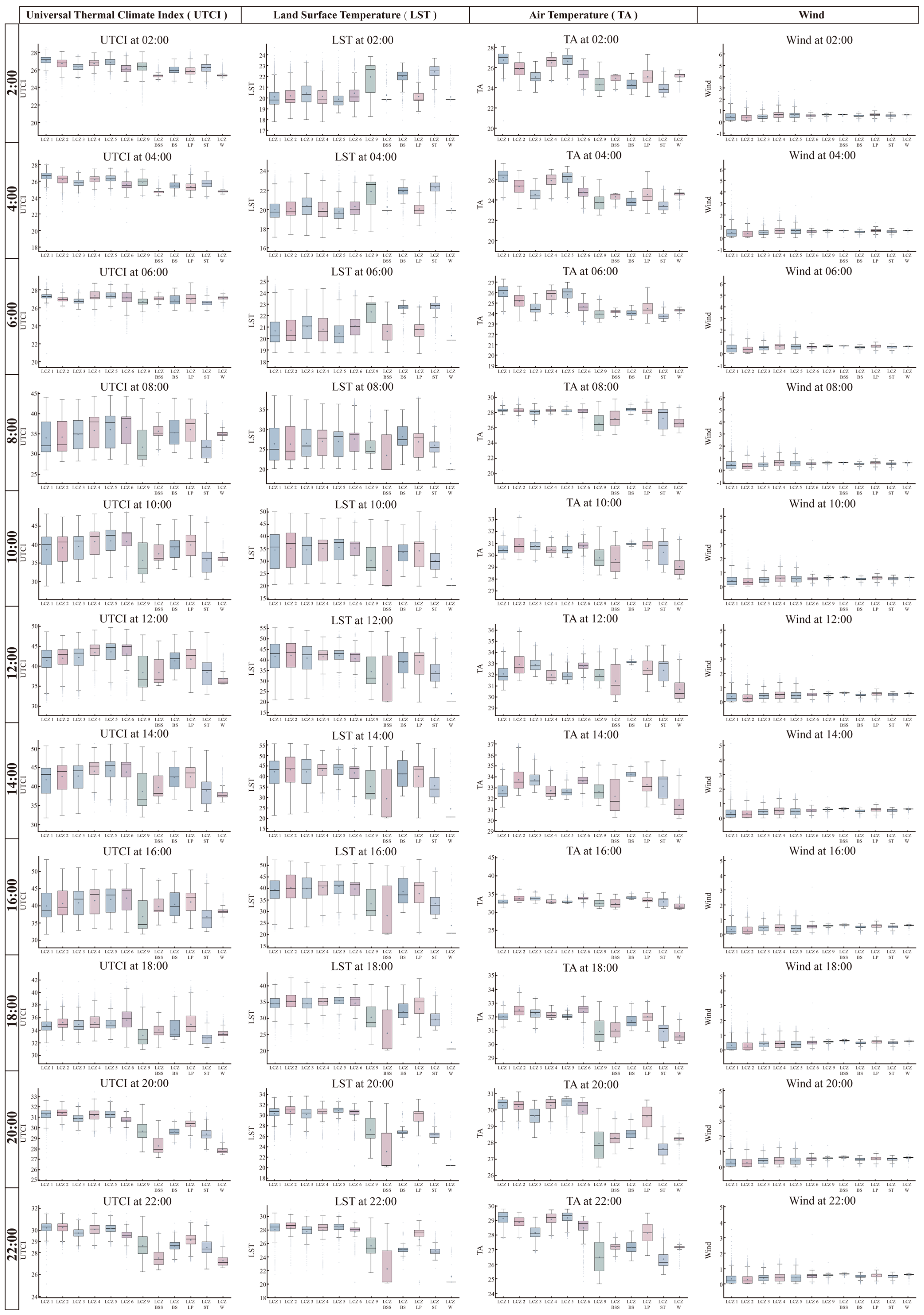
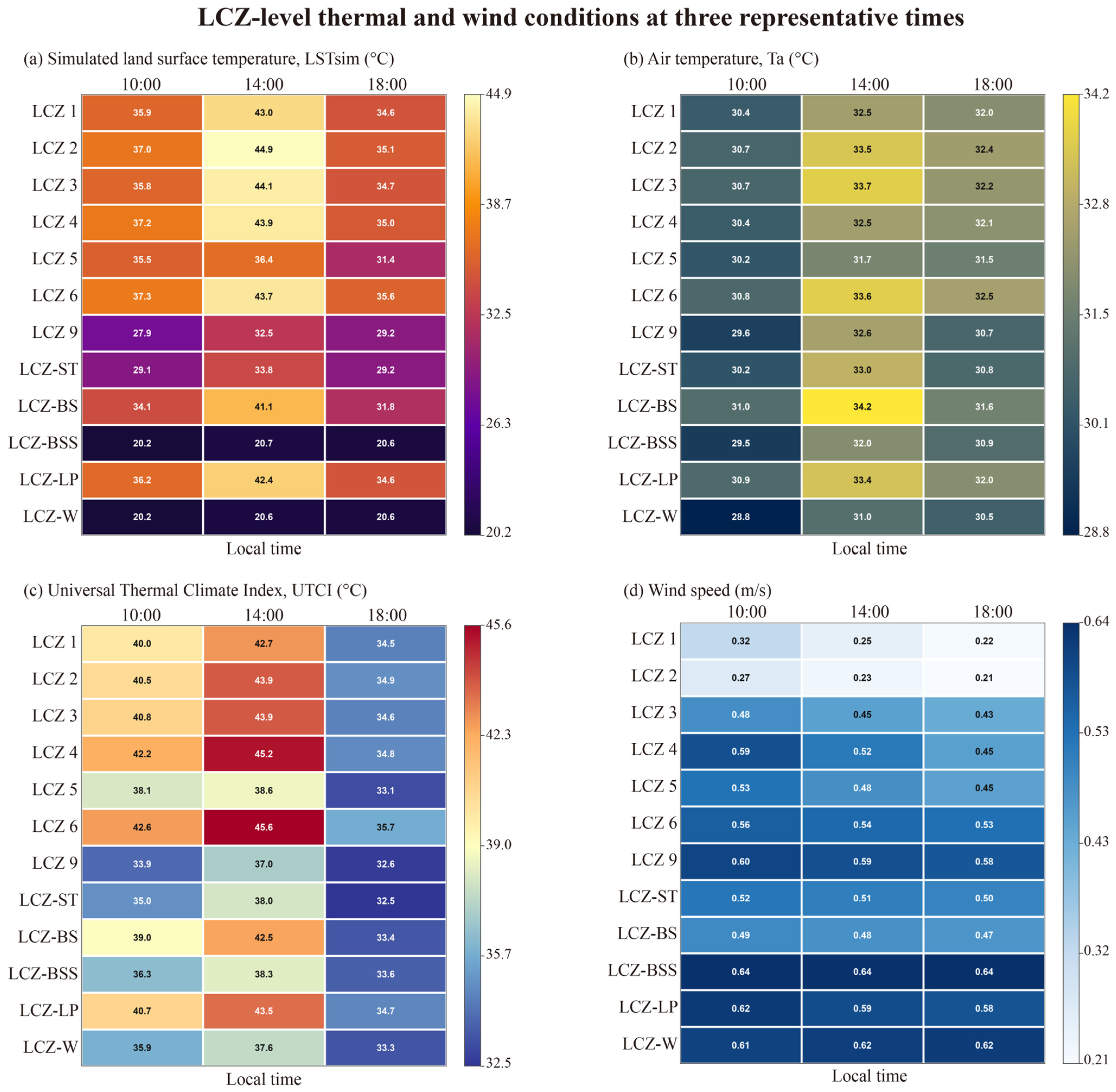
The ENVI-met diurnal profiles shown in Figure 7 display LCZ-dependent variation in simulated land surface temperature (LSTsim), near-surface air temperature (Ta), wind speed, and simulated UTCI. To improve readability, Figure 8 summarizes the LCZ-level values at 10:00, 14:00, and 18:00 using the median of the two plot-level spatial medians within each LCZ. Complete plot-level spatial maps for all 24 representative plots are provided in Supplementary Figures S1–S4. An extended five-time LSTsim display, including 12:00 and 16:00 and the corresponding satellite reference maps, is provided in Supplementary Figure S6. Differences among LCZs were relatively weak during the nighttime and early morning period, particularly from 02:00 to 06:00, and the descriptive separation increased after sunrise, with the widest distributional ranges occurring between 12:00 and 16:00. The clearest descriptive separation occurred around 14:00, which was selected as the key diagnostic model time slice, while satellite comparisons were conducted separately using the actual ECOSTRESS acquisition times. Because formal inference was based on only 24 plot-level units, these profiles and summaries are interpreted descriptively and are not used alone to claim statistically significant LCZ differences.

Figure 8 shows that the LCZ-level thermal contrasts were most pronounced at 14:00. Several built LCZs exhibited relatively high LSTsim and simulated UTCI, whereas LCZ-W and LCZ-BSS showed the lowest LSTsim values. However, the rankings were not identical across variables. For example, LCZ6 and LCZ4 showed high simulated UTCI at 14:00, while LCZ-BSS and LCZ-W exhibited relatively high wind speeds. This divergence indicates that surface temperature alone does not reproduce the combined pattern of simulated pedestrian heat exposure. These comparisons are descriptive because each LCZ summary is based on two representative plots. The complete spatial distributions underlying these summaries are shown in Supplementary Figures S1–S4.

Quality-control flag: LCZ-BSS LSTsim was 20.2, 20.7, and 20.6 °C at 10:00, 14:00, and 18:00, nearly identical to LCZ-W and markedly below simulated air temperature. This physically unusual pattern is displayed for transparency but is excluded from mechanistic and proxy-efficacy interpretation.

At 14:00, grid-/subsite-level Kruskal–Wallis tests showed descriptive distributional separation among LCZ types for LST, air temperature, wind speed, and simulated UTCI. Because these tests used within-plot grid observations, their H statistics and p-values may be inflated by spatial autocorrelation and are therefore treated only as descriptive evidence of within-scene spatial differentiation, not as formal independent inference.

Formal LCZ-level comparison was conducted using plot-aggregated simulated UTCI values, with the 24 representative plots treated as the primary statistical units. At this level, the Kruskal–Wallis test did not reach statistical significance among LCZ types (H = 15.80, df = 11, p = 0.149). However, the design included only two plots per LCZ type, which limited statistical power and resulted in deliberately conservative plot-level inference.

Accordingly, the study does not claim statistically significant UTCI differences among all LCZ classes. Cell-level patterns are descriptive, and the plot-level perturbation analyses cannot overcome two plots per LCZ. CPE is used only as a conceptual label for juxtaposing association strength, mismatch direction, and cross-scene consistency. It is not an operational proxy, efficacy classification, or statistically confirmed LCZ hierarchy.

3.2. LCZ-Dependent Association Between LST and Simulated UTCI

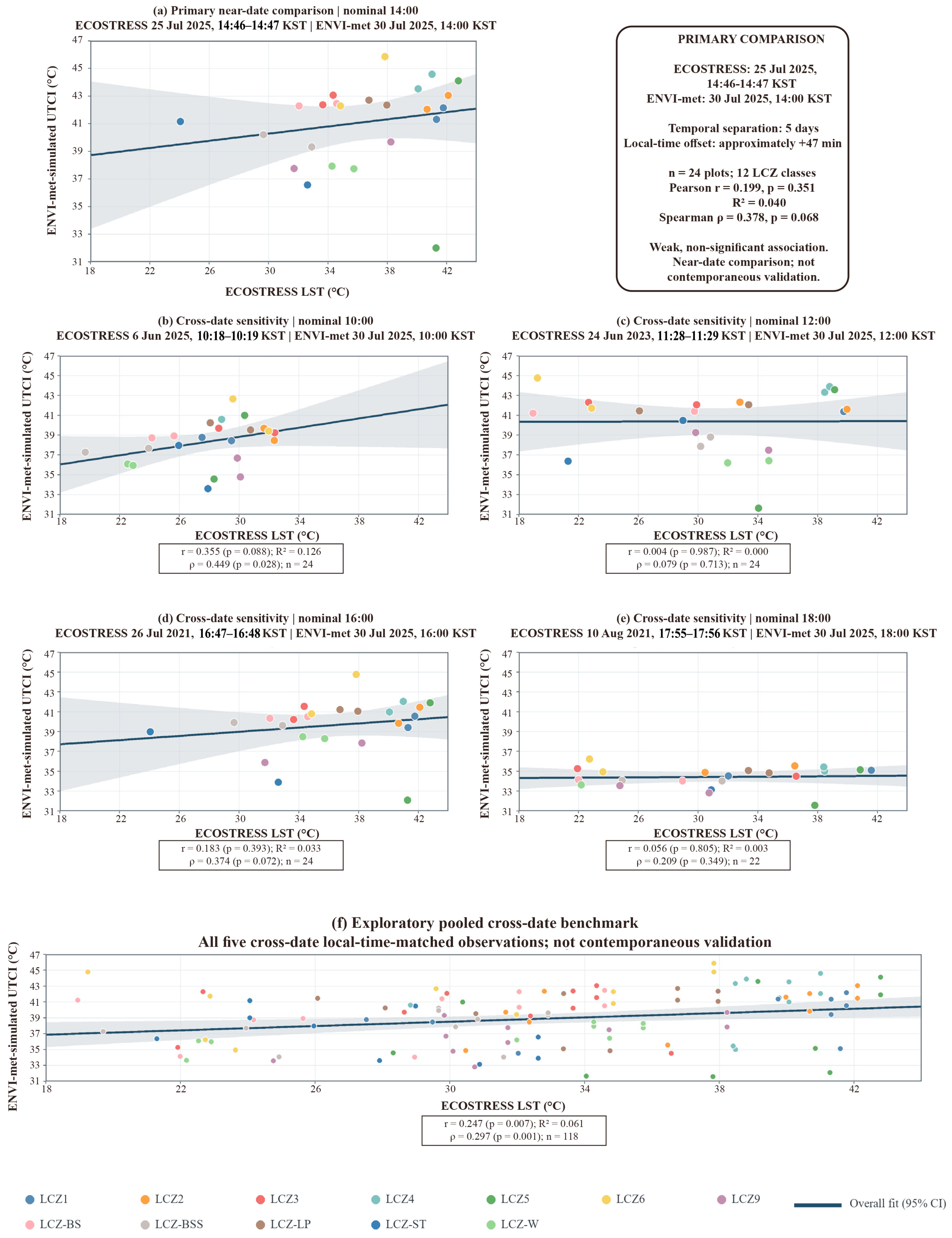
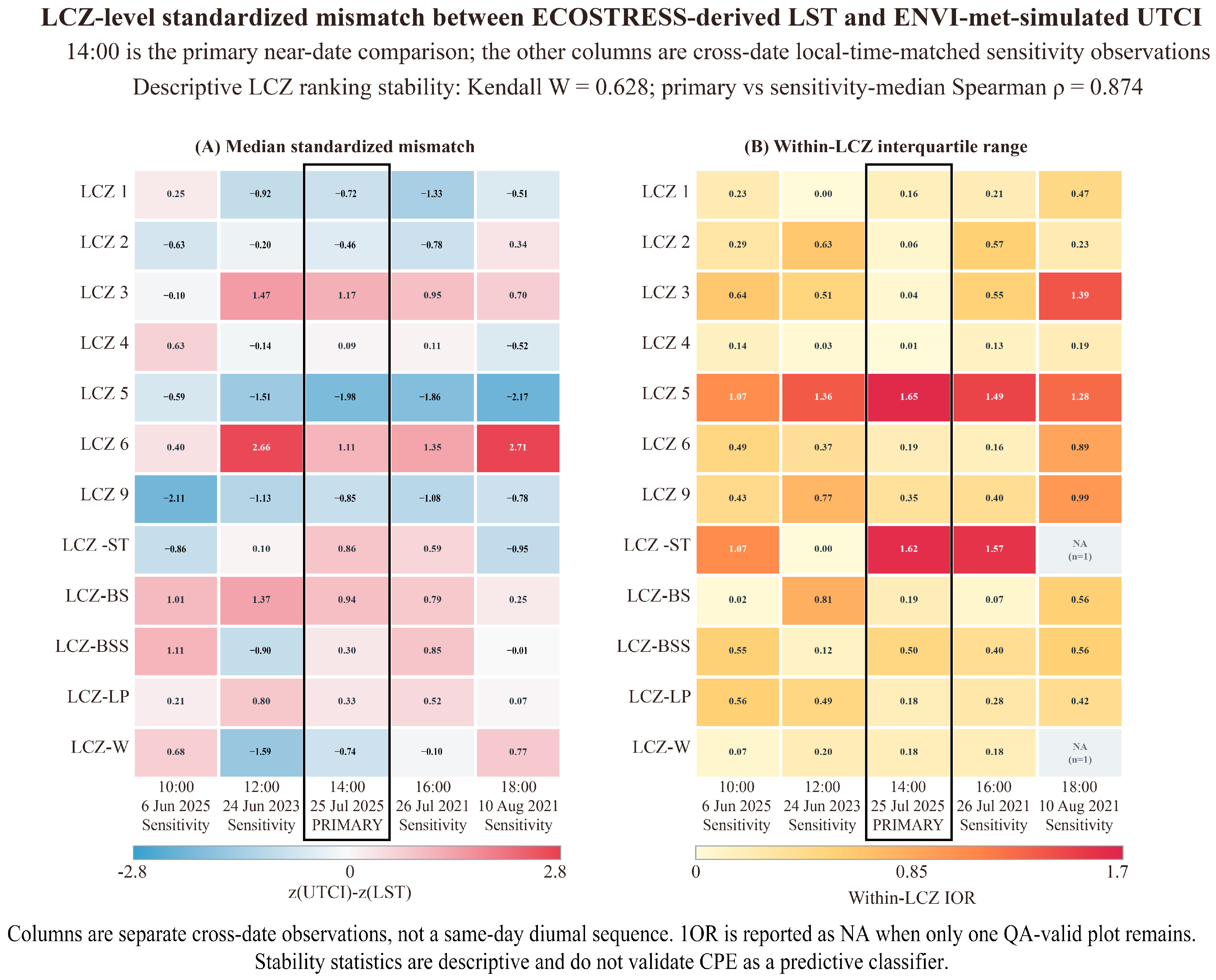
The primary analysis used the 25 July 2025 ECOSTRESS acquisition (14:46:37 KST) and the 30 July 2025 14:00 ENVI-met output. For the 24 plots, the corrected source-level LST–UTCI association was weak and non-significant (Pearson r = 0.199, p = 0.351, R² = 0.040; Spearman ρ = 0.378, p = 0.068). The LCZ median standardized mismatch ranged from −1.98 in LCZ5 to +1.17 in LCZ3, with LCZ6 (+1.11) and LCZ-BS (+0.94) also showing positive mismatch. These values remain descriptive rather than confirmatory.

At Seoul ASOS 108, the primary overpass differed from the matched 30 July 14:00 station reference by +0.3 °C in Ta, +1.1 percentage points in RH, +0.3 m/s in wind speed, and −4/8 in cloud amount. The small Ta, RH, and wind departures support its primary role, while the cloud difference and five-day separation preclude contemporaneous validation.

The four remaining acquisitions were separate cross-date sensitivity observations, with scene-specific R² values of 0.126, 0.000, 0.033, and 0.003. The pooled five-scene benchmark comprised 118 observations (r = 0.247, unadjusted Pearson p = 0.007, R² = 0.061). Because the same plots recur across scenes, that p value assumes independence and is descriptive only; the plot-cluster-robust regression gave p = 0.015, and the scene-adjusted slope gave p = 0.371 (Table S6).

The source-pair audit traced all 120 expected plot × scene keys. It corrected the legacy BS/BSS and water-sample aliases and identified two 18:00 LST records with zero effective pixels; these were excluded rather than replaced, leaving 118 QA-valid observations in 24 plot clusters (Table S5).

The pooled LST slope was 0.136 °C UTCI per °C LST (plot-cluster-robust 95% CI 0.029 to 0.244; p = 0.015). After scene fixed effects and within-scene centering, the slope decreased to 0.060 (95% CI −0.075 to 0.195; p = 0.371; partial R² = 0.015). The LST × scene interaction was not significant (cluster-robust Wald F(4,23) = 2.070, p = 0.118). Only the 10:00 scene-specific slope excluded zero (0.232; 95% CI 0.079 to 0.384; p = 0.005); the other four scene-specific intervals crossed zero (Table S6).

The primary and scene-adjusted results do not demonstrate stable proxy performance. Associations varied across scenes, the adjusted interval crossed zero, and UTCI depends on modeled radiation, wind, humidity, and air temperature that LST does not directly observe.

Across the four sensitivity scenes, R² ranged from 0.000 to 0.126, and none of the five scene-specific Pearson tests was significant. Figure 9 reports ordinary scene-wise correlations; the pooled panel’s p values are unadjusted for repeated plots. Cluster-robust and scene-adjusted inference is reported in Table S6.

Scatter and mismatch direction differed across plots and scenes, but with two plots per LCZ the study cannot estimate distinct proxy-performance regimes. Radiation, wind, shading, and surface cover remain plausible contextual explanations only; they were not experimentally isolated, and UTCI was not independently validated.

Satellite LST remains informative for surface thermal gradients, but this analysis does not estimate a validated conversion, classification threshold, or misclassification rate for pedestrian exposure. Any LCZ-sensitive use should therefore remain descriptive and explicitly model-dependent.

3.3. Bias Between Satellite-Derived LST and ENVI-Met Simulated LST

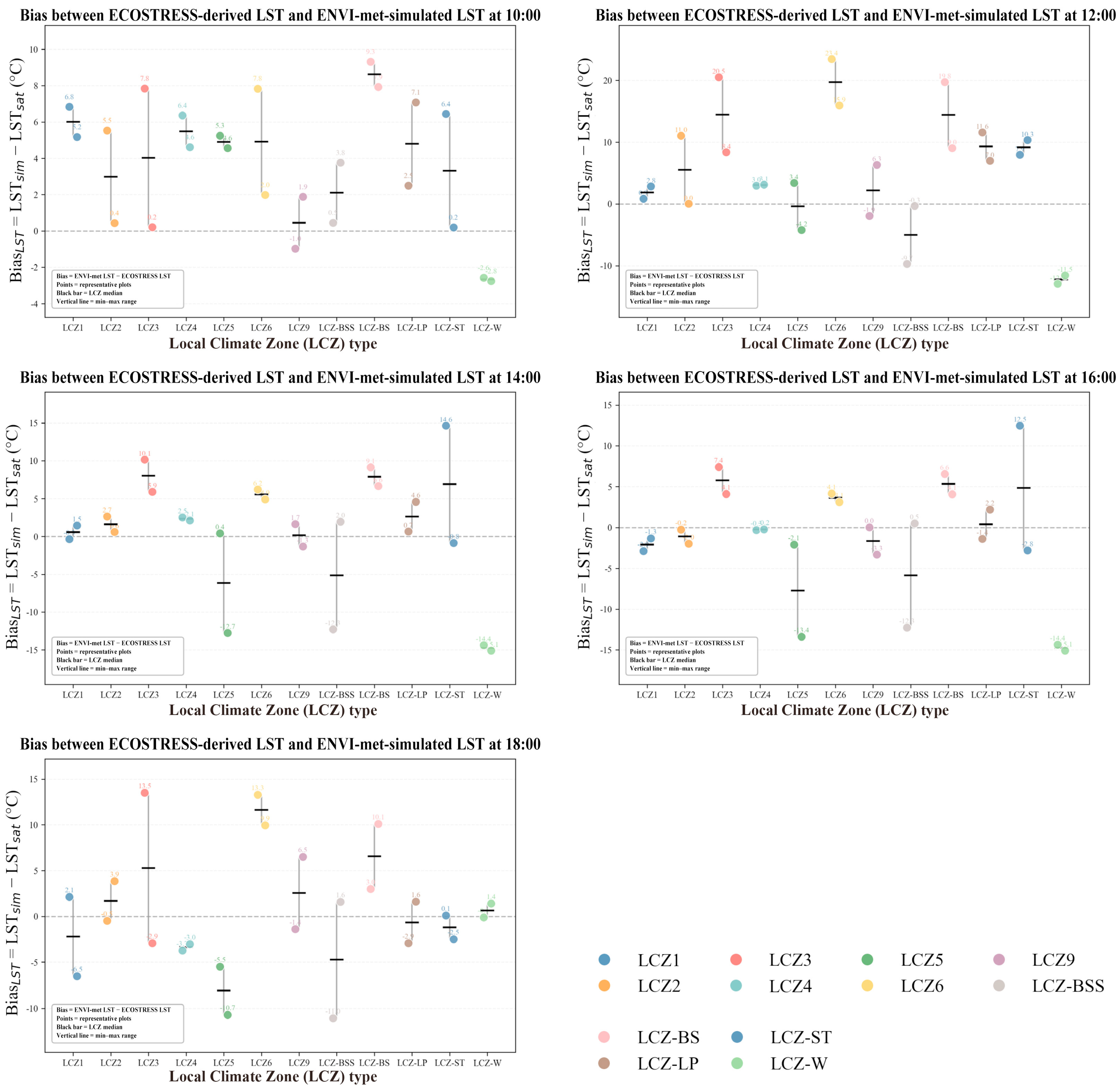
The comparison between satellite-derived LST and ENVI-met-simulated LST revealed systematic deviations between the two surface-temperature products. The direction and magnitude of this bias varied across LCZ types and nominal local-time matches, indicating that satellite-observed and model-simulated LST should not be treated as interchangeable. Built LCZs generally exhibited larger deviations than natural and water-related LCZs, reflecting the higher heterogeneity of surface materials, shading patterns, thermal storage, and radiative geometry in urban built environments.

Across the nominal local-time matches, larger satellite–model biases were observed in several of the 12:00–16:00 comparisons. However, because the ECOSTRESS scenes were acquired on different dates and years, this pattern cannot be attributed solely to time of day. Differences in weather conditions, antecedent surface moisture, vegetation state, viewing geometry, and surface energy balance may also contribute. ECOSTRESS thermal observations represent the instantaneous radiative response of exposed surfaces, whereas ENVI-met estimates surface temperature through local energy-balance calculations incorporating material properties, vegetation, shading, and near-surface atmospheric exchange. The LCZ-specific bias is summarized in Figure 10.

Bias was calculated as ENVI-met-simulated LST minus satellite-derived LST. Colored points represent representative LCZ plots, black horizontal bars indicate LCZ-level median bias, and vertical lines show the min–max range within each LCZ. Positive values indicate that ENVI-met-simulated LST exceeds satellite-derived LST, whereas negative values indicate the opposite.

This comparison has two implications. First, uncertainty exists before LST is related to simulated pedestrian heat exposure: satellite-based and model-based surface temperatures are affected by different observational and modeling assumptions. Second, the translation from satellite-derived LST to simulated UTCI may accumulate uncertainty from surface-temperature retrieval, microclimate modeling, and the unvalidated MRT and wind components of UTCI. The LST–UTCI mismatch is therefore interpreted as a cross-scale representational problem, not as direct evidence of a measured comfort response.

3.4. Standardized Mismatch Between LST and Simulated UTCI Across LCZs

Having established that satellite-derived and model-simulated LST differ at the surface level (Section 3.3), this section examines how the satellite surface signal is associated with simulated UTCI. A standardized mismatch index was calculated between satellite-derived LST anomalies and simulated UTCI anomalies. The index displayed LCZ-dependent descriptive variation rather than uniform variation around zero, indicating that the relationship between surface thermal anomalies and modeled pedestrian exposure may be conditioned by LCZ context. This result does not establish causal effects or statistically confirmed differences among all LCZ classes.

The median standardized mismatch varied among LCZ types. Positive mismatch values indicate that simulated UTCI was higher than would be inferred from LST anomalies alone, whereas negative values indicate that LST anomalies were higher than simulated UTCI anomalies. Larger mismatch values occurred in several nominal midday and early-afternoon comparisons. Because the scenes were acquired on different dates, these are interpreted as recurring cross-scene spatial patterns rather than a continuous same-day temporal trajectory.

Several LCZs, including LCZ3, LCZ6, and LCZ-BS, showed positive mismatch in multiple comparisons, meaning that simulated UTCI was relatively higher than the corresponding LST anomaly. High radiative exposure, limited shade, lower simulated wind speed, and surface–air exchange are plausible contextual explanations, but their causal contributions were not separately tested. In contrast, LCZ5, LCZ9, and some observations in LCZ-ST and LCZ-W showed negative mismatch. These descriptive patterns suggest that LST and simulated pedestrian exposure are linked through LCZ-specific conditions involving radiation, ventilation, shading, and surface cover.

Panel B of Figure 11 shows the interquartile range of the two plot-level mismatch summaries available for each LCZ (or NA when only one plot remained). With n = 2, this is only a compact description of between-plot spread; it cannot establish substantial intra-LCZ heterogeneity or population variability. Future studies should sample more independent plots and measure morphology directly.

Panel A shows the LCZ median of the available plot-level mismatch values, and Panel B shows the corresponding descriptive two-plot interquartile range. Positive values indicate that simulated UTCI is relatively higher than implied by the LST anomaly, and negative values indicate the opposite. Columns are separate cross-date observations; neither panel provides confirmatory LCZ inference.

3.5. Cross-Scene and Plot-Level Robustness

The primary 14:00 mismatch ranking agreed strongly with the sensitivity-scene median (Spearman ρ = 0.874), and the five scene-wise rankings were concordant (Kendall W = 0.628). Direction was invariant for LCZ5, LCZ6, LCZ9, LCZ-BS, and LCZ-LP; LCZ4, LCZ-ST, LCZ-BSS, and LCZ-W retained the modal direction in three of five scenes (Tables S3 and S4; Figure S5).

All 24 leave-one-plot-out slopes were positive (0.035–0.105), and the minimum rank correlation was ρ = 0.909. These values are mechanically constrained: deleting one plot changes at most one LCZ median while the other 11 remain fixed. The two-plot-per-LCZ bootstrap slope range crossed zero (−0.033 to 0.151). These diagnostics describe sensitivity to the observed plots only and are not used to claim sign certainty, population confidence, or CPE robustness (Table S8).

3.6. Ventilation Patterns and Their Association with LST–UTCI Divergence

Simulated wind speed varied across LCZs: compact built classes generally had lower pedestrian-level values, which coincided with higher simulated UTCI relative to LST. The 14:00 grid/subsite Kruskal–Wallis test was significant (p < 0.001, η² = 0.266), but spatial dependence, the use of wind as a UTCI input, and the absence of direct wind validation limit this to a descriptive association, not evidence of a causal ventilation mechanism.

4. Discussion

4.1. Hypothesized Mechanisms Associated with LST–UTCI Divergence

The LST–UTCI relationship is indirect: satellite LST represents surface radiative conditions, whereas simulated UTCI combines modeled air temperature, mean radiant temperature (MRT), wind, and humidity. Because UTCI and its MRT and wind inputs were not independently field validated, the pathways below are hypotheses. In compact built LCZs, exposed roofs and pavements dominate satellite LST, while canyon geometry, sky-view factor, orientation, and shade modify pedestrian-level modeled radiation. This radiative decoupling is consistent with prior evidence [19,53,54] but requires direct radiation or globe-temperature validation.

Modeled ventilation and latent heat provide two additional interpretations. Wind can alter convective exchange without being represented by LST, while vegetation and water may suppress surface temperature through evapotranspiration and simultaneously alter humidity. These processes could make similar LST values coincide with different simulated UTCI values, but this study neither validated wind nor isolated energy partitioning experimentally.

Accordingly, LST should be interpreted as a conditional indicator of surface thermal intensity rather than a direct measure of heat stress. Although the analysis used ECOSTRESS, the same caution applies to Landsat and other thermal platforms. Direct MRT, radiation, three-dimensional wind, and humidity measurements are needed to test the proposed pathways.

4.2. A Conceptual CPE Heuristic for Organizing Observed Mismatch

The Conditional Proxy Efficacy (CPE) construct is a conceptual organizing heuristic. It juxtaposes scene-wise association, mismatch direction, and cross-scene consistency, but it has no fitted equation, threshold, calibration sample, or out-of-sample validation. It therefore cannot identify when LST is an effective proxy.

The present sample does not support High, Moderate, or Low efficacy categories, nor defensible LCZ assignments to such categories. Those labels and operational claims have been removed. The observed values are retained only to formulate testable hypotheses for larger, independently validated studies.

Future operationalization would require prespecified thresholds, more independent plots per LCZ, temporally coincident satellite and field observations, direct MRT and wind validation, and external testing across cities. LCZ-W and the flagged LCZ-BSS case remain model-only descriptive contexts.

4.3. Implications for the Surface Urban Heat Island Paradigm

The LST–UTCI mismatch qualifies, rather than negates, the surface urban heat island paradigm. Satellite LST remains valuable for monitoring surface thermal contrasts, but the present model-based comparison shows that surface rankings and simulated exposure rankings need not coincide. It does not provide a validated basis for re-prioritizing health-risk interventions.

4.4. Synthesis: From Proxy Substitution to Conditional Model-Based Inference

The raw pooled association was weak (r = 0.247, unadjusted p = 0.007, R² = 0.061, n = 118), and the plot-cluster-robust pooled slope had p = 0.015. After scene adjustment, the LST slope was 0.060, and its 95% CI crossed zero. Scene-specific R² values ranged from 0.000 to 0.126. These cross-date results do not establish a diurnal trend or stable screening capability.

The pooled LST-only benchmark explained 6.1% of UTCI variance; thus, 93.9% was not explained by LST alone. This remainder must not be interpreted as evidence of hidden physical mechanisms. The separate multivariable Shapley diagnostic in Table S7 allocates the full-model explained variance and leaves a residual share of 14.3% [55]. These shares are retained only as supplementary descriptive model diagnostics. Because simulated air temperature and wind are direct inputs to simulated UTCI, their allocation is partly circular; correlations among predictor blocks further preclude interpretation as independent mechanistic or causal contributions.

Observed divergence may involve radiative geometry, modeled ventilation, humidity, and surface energy partitioning, but none was independently identified as causal. CPE is therefore retained only as a hypothesis-generating label. LST remains valuable for surface monitoring; direct, field-validated MRT, wind, and UTCI are required for human-scale heat-risk assessment.

4.5. Limitations and Future Research

Several limitations should be acknowledged. First, the ECOSTRESS observations were not acquired on the ENVI-met simulation date of 30 July 2025. Although the scenes were assigned to the nearest of five preselected ENVI-met comparison outputs according to actual local acquisition time, the acquisitions span 2021–2025 and do not represent a continuous same-day diurnal cycle. Weather, antecedent moisture, vegetation condition, surface energy balance, and viewing geometry may affect the observed mismatch. The comparisons are therefore tests of cross-date spatial and LCZ-dependent pattern correspondence rather than contemporaneous validation of absolute temperature. Second, ECOSTRESS had a native spatial resolution of 70 m, whereas ENVI-met used a 5 m grid, so scale mismatch may obscure roofs, roads, vegetation, shaded canyons, and courtyards. Future studies should prioritize temporally coincident observations and very-high-resolution UAV or airborne thermal imagery.

The reference-station comparison confirms that the primary scene was closest to the simulation-day Ta, RH, and wind conditions, but cloud amount still differed by four oktas; the sensitivity scenes showed larger departures in one or more meteorological variables. These observations contextualize rather than remove the cross-date confounding.

Third, and most importantly, ENVI-met validation was limited to air temperature and relative humidity. UTCI itself was not independently validated against field-observed mean radiant temperature, wind speed, globe temperature, short- and long-wave radiation, physiological responses, or subjective thermal votes. Good agreement for Ta and RH cannot therefore be interpreted as validation of simulated UTCI. Throughout this study, UTCI should be understood as a model-based heat-exposure indicator used for relative LCZ comparison, not as a directly measured or clinically validated estimate of human thermal stress. Associations involving wind, radiation, morphology, and mismatch are observational and model-based and do not establish causal effects. Future work should jointly validate Ta, RH, wind speed, globe temperature or MRT, and radiation fluxes, and should compare simulated UTCI with field-derived UTCI and, where feasible, human thermal-response observations.

This validation gap is especially consequential in urban canyons. Errors in shading, view factors, surface radiative exchange, and short- and long-wave fluxes propagate into Tmrt, while errors under low pedestrian-level wind alter convective cooling. Because Tmrt and wind enter UTCI nonlinearly, compound bias can shift absolute UTCI and may also alter LCZ ordering. The present UTCI and CPE results are therefore suitable only for relative, exploratory comparison until coordinated MRT, radiation, globe-temperature, and wind measurements are available.

Fourth, formal inference was based on 24 plots with only two plots per LCZ. Leave-one-plot-out and stratified resampling are discrete perturbation checks, not population-level uncertainty estimates; high rank agreement is partly expected because 11 LCZ medians remain unchanged in each deletion. Fifth, the LCZ-BSS surface-temperature pattern is physically unusual, so that class is flagged and is not used for mechanistic or proxy-efficacy claims. Sixth, the study examined one summer scenario in Seoul. Multi-season, multi-city, and larger-sample validation is required.

5. Conclusions

This study tested whether ECOSTRESS-derived LST showed a stable association with ENVI-met-simulated UTCI across 24 Seoul LCZ plots. UTCI was treated as a model-based indicator, not a direct observation of thermal comfort or health outcome. One near-date scene was primary; four cross-date scenes were sensitivity observations.

The primary association was weak and non-significant (r = 0.199, p = 0.351, R² = 0.040, n = 24). Across 118 QA-valid plot × scene records, the raw pooled benchmark remained weak (R² = 0.061), while the scene-adjusted slope was 0.060 with a cluster-robust 95% CI of −0.075 to 0.195. The LST × scene interaction and plot-level LCZ differences were not significant. The study therefore did not demonstrate stable LST screening performance for simulated pedestrian exposure.

The contribution is a source-audited, explicitly limited cross-platform comparison and a conceptual CPE heuristic for organizing future hypotheses. CPE is not a validated classifier, efficacy scale, or transferable LCZ ranking. Larger samples, temporally coincident observations, access to supporting model configuration, and direct validation of MRT, wind, radiation, and UTCI are prerequisites for operational use.

References

1. Intergovernmental Panel on Climate Change (IPCC). The IPCC Sixth Assessment Report on Climate Change Impacts. Popul. Dev. Rev. 2022, 48, 629–633. [Google Scholar] [CrossRef] [Scilit]
2. Mora, C.; Dousset, B.; Caldwell, I.R.; Powell, F.E.; Geronimo, R.C.; Bielecki, C.R.; Counsell, C.W.W.; Dietrich, B.S.; Johnston, E.T.; Louis, L.V.; et al. Global risk of deadly heat. Nat. Clim. Change 2017, 7, 501–506. [Google Scholar] [CrossRef] [Scilit]
3. Vicedo-Cabrera, A.M.; Scovronick, N.; Sera, F.; Roye, D.; Schneider, R.; Tobias, A.; Astrom, C.; Guo, Y.; Honda, Y.; Hondula, D.M.; et al. The burden of heat-related mortality attributable to recent human-induced climate change. Nat. Clim. Change 2021, 11, 492–500. [Google Scholar] [CrossRef] [Scilit]
4. An, S.; Dedekorkut-Howes, A. The Heat Is on: How Well Are Densely Populated Korean Cities Adapting to Increased Temperatures and Urban Heat Island Effect? Environments 2025, 12, 87. [Google Scholar] [CrossRef] [Scilit]
5. Manoli, G.; Fatichi, S.; Schlapfer, M.; Yu, K.; Crowther, T.W.; Meili, N.; Burlando, P.; Katul, G.G.; Bou-Zeid, E. Magnitude of urban heat islands largely explained by climate and population. Nature 2019, 573, 55–60. [Google Scholar] [CrossRef] [Scilit] [PubMed]
6. Li, Z.-L.; Tang, B.-H.; Wu, H.; Ren, H.; Yan, G.; Wan, Z.; Trigo, I.F.; Sobrino, J.A. Satellite-derived land surface temperature: Current status and perspectives. Remote Sens. Environ. 2013, 131, 14–37. [Google Scholar] [CrossRef] [Scilit]
7. Reiners, P.; Sobrino, J.; Kuenzer, C. Satellite-Derived Land Surface Temperature Dynamics in the Context of Global Change—A Review. Remote Sens. 2023, 15, 1857. [Google Scholar] [CrossRef] [Scilit]
8. Weng, Q. Thermal infrared remote sensing for urban climate and environmental studies: Methods, applications, and trends. ISPRS J. Photogramm. Remote Sens. 2009, 64, 335–344. [Google Scholar] [CrossRef] [Scilit]
9. Kenawy, A.; Muse, N.; Clement, A.; Mach, K.J. Daytime land surface temperature and its limits as a proxy for surface air temperature in a subtropical, seasonally wet region. PLoS Clim. 2024, 3, e0000278. [Google Scholar] [CrossRef] [Scilit]
10. Peng, S.; Piao, S.; Ciais, P.; Friedlingstein, P.; Ottle, C.; Breon, F.M.; Nan, H.; Zhou, L.; Myneni, R.B. Surface urban heat island across 419 global big cities. Environ. Sci. Technol. 2012, 46, 696–703. [Google Scholar] [CrossRef] [Scilit] [PubMed]
11. Zhou, D.; Xiao, J.; Bonafoni, S.; Berger, C.; Deilami, K.; Zhou, Y.; Frolking, S.; Yao, R.; Qiao, Z.; Sobrino, J.A. Satellite Remote Sensing of Surface Urban Heat Islands: Progress, Challenges, and Perspectives. Remote Sens. 2018, 11, 48. [Google Scholar] [CrossRef] [Scilit]
12. Maroni, D.; Cardoso, G.T.; Neckel, A.; Maculan, L.S.; Oliveira, M.L.S.; Bodah, E.T.; Bodah, B.W.; Santosh, M. Land surface temperature and vegetation index as a proxy to microclimate. J. Environ. Chem. Eng. 2021, 9, 105796. [Google Scholar] [CrossRef] [Scilit]
13. Naserikia, M.; Hart, M.A.; Nazarian, N.; Bechtel, B.; Lipson, M.; Nice, K.A. Land surface and air temperature dynamics: The role of urban form and seasonality. Sci. Total Environ. 2023, 905, 167306. [Google Scholar] [CrossRef] [Scilit] [PubMed]
14. Tuholske, C.; Caylor, K.; Funk, C.; Verdin, A.; Sweeney, S.; Grace, K.; Peterson, P.; Evans, T. Global urban population exposure to extreme heat. Proc. Natl. Acad. Sci. USA 2021, 118, e2024792118. [Google Scholar] [CrossRef] [Scilit] [PubMed]
15. Li, Y.; Zhang, Y.; Kong, Y.; Wang, Y.; Zhou, M.; Chang, Y.; Li, J. Landscape patterns and diurnal thermal effects of golf courses in urban and suburban settings. Urban Clim. 2026, 65, 102763. [Google Scholar] [CrossRef] [Scilit]
16. Chen, X.; Zhang, Y.; Song, Z.; Wang, Z.; Lin, H.; Lan, T.; Shao, J.; Lei, T.; Jin, R.; Li, J. Street Orientation, Aspect Ratio, and Tree Species Interactions on Heat Exposure in Temperate Monsoon Climate. Sustainability 2026, 18, 3177. [Google Scholar] [CrossRef] [Scilit]
17. Li, Y.; Zhang, Y.; Wang, Y.; Song, Z.; Zhou, Z.; Ding, L.; Chen, C.; Jin, X.; Cheng, Y. Assessing thermal comfort for the elderly in historical districts and proposing adaptive urban design strategies: A case study in Zhenjiang, China. Landsc. Ecol. Eng. 2024, 21, 29–46. [Google Scholar] [CrossRef] [Scilit]
18. Zhang, Y.; Kong, Y.; Chen, C.; Lin, J.; Lin, D.; Zhang, Y.; Li, Y. The impact of urban morphology on thermal environment under extreme heat: A case study in Nanjing, China. Urban Clim. 2024, 58, 102178. [Google Scholar] [CrossRef] [Scilit]
19. Briegel, F.; Pinto, J.G.; Christen, A. Is satellite land surface temperature an appropriate proxy for intra-urban variability of daytime heat stress? Remote Sens. Environ. 2025, 331, 115045. [Google Scholar] [CrossRef] [Scilit]
20. Ali-Toudert, F.; Mayer, H. Numerical study on the effects of aspect ratio and orientation of an urban street canyon on outdoor thermal comfort in hot and dry climate. Build. Environ. 2006, 41, 94–108. [Google Scholar] [CrossRef] [Scilit]
21. Bansal, P.; Quan, S.J. Relationships between building characteristics, urban form and building energy use in different local climate zone contexts: An empirical study in Seoul. Energy Build. 2022, 272, 112335. [Google Scholar] [CrossRef] [Scilit]
22. Korean Statistical Information Service. Economically Active Population by Age (Table ID: DT_1ES3B32S); KOSIS: Korean Statistical Information Service: Daejeon, Republic of Korea, 2023.
23. Lee, S.-H.; Baik, J.-J. Statistical and dynamical characteristics of the urban heat island intensity in Seoul. Theor. Appl. Climatol. 2010, 100, 227–237. [Google Scholar] [CrossRef] [Scilit]
24. Park, K.; Jin, H.-G.; Baik, J.-J. Contrasting interactions between urban heat islands and heat waves in Seoul, South Korea, and their associations with synoptic patterns. Urban Clim. 2023, 49, 101524. [Google Scholar] [CrossRef] [Scilit]
25. Bechtel, B.; Alexander, P.; Böhner, J.; Ching, J.; Conrad, O.; Feddema, J.; Mills, G.; See, L.; Stewart, I. Mapping Local Climate Zones for a Worldwide Database of the Form and Function of Cities. ISPRS Int. J. Geo-Inf. 2015, 4, 199–219. [Google Scholar] [CrossRef] [Scilit]
26. Oke, T.R.; Stewart, I.D. Local Climate Zones for Urban Temperature Studies. Bull. Am. Meteorol. Soc. 2012, 93, 1879–1900. [Google Scholar] [CrossRef] [Scilit]
27. Núñez Peiró, M.; Sánchez-Guevara Sánchez, C.; Neila González, F.J. Source area definition for local climate zones studies. A systematic review. Build. Environ. 2019, 148, 258–285. [Google Scholar] [CrossRef] [Scilit]
28. Demuzere, M.; Kittner, J.; Martilli, A.; Mills, G.; Moede, C.; Stewart, I.D.; van Vliet, J.; Bechtel, B. A global map of local climate zones to support earth system modelling and urban-scale environmental science. Earth Syst. Sci. Data 2022, 14, 3835–3873. [Google Scholar] [CrossRef] [Scilit]
29. Puche, M.; Vavassori, A.; Brovelli, M.A. Insights into the Effect of Urban Morphology and Land Cover on Land Surface and Air Temperatures in the Metropolitan City of Milan (Italy) Using Satellite Imagery and In Situ Measurements. Remote Sens. 2023, 15, 733. [Google Scholar] [CrossRef] [Scilit]
30. Wu, J.; Liu, C.; Wang, H. Analysis of Spatio-temporal patterns and related factors of thermal comfort in subtropical coastal cities based on local climate zones. Build. Environ. 2022, 207, 108568. [Google Scholar] [CrossRef] [Scilit]
31. Yang, J.; Ren, J.; Sun, D.; Xiao, X.; Xia, J.; Jin, C.; Li, X. Understanding land surface temperature impact factors based on local climate zones. Sustain. Cities Soc. 2021, 69, 102818. [Google Scholar] [CrossRef] [Scilit]
32. Cai, Z.; Han, G.; Chen, M. Do water bodies play an important role in the relationship between urban form and land surface temperature? Sustain. Cities Soc. 2018, 39, 487–498. [Google Scholar] [CrossRef] [Scilit]
33. Wu, Z.; Zhang, Y. Water Bodies’ Cooling Effects on Urban Land Daytime Surface Temperature: Ecosystem Service Reducing Heat Island Effect. Sustainability 2019, 11, 787. [Google Scholar] [CrossRef] [Scilit]
34. Hulley, G.C.; Freepartner, R. ECOsystem Spaceborne Thermal Radiometer Experiment on Space Station (ECOSTRESS) Mission: Level 2 Product User Guide v002; Jet Propulsion Laboratory, California Institute of Technology: Pasadena, CA, USA, 2024. [Google Scholar]
35. Hook, S.; Hulley, G. ECOSTRESS Tiled Land Surface Temperature and Emissivity Instantaneous L2 Global 70 m V002 (ECO_L2T_LSTE.002); NASA EOSDIS Land Processes Distributed Active Archive Center (LP DAAC): Sioux Falls, SD, USA, 2023. [CrossRef]
36. Hulley, G.C.; Göttsche, F.M.; Rivera, G.; Hook, S.J.; Freepartner, R.J.; Martin, M.A.; Cawse-Nicholson, K.; Johnson, W.R. Validation and Quality Assessment of the ECOSTRESS Level-2 Land Surface Temperature and Emissivity Product. IEEE Trans. Geosci. Remote Sens. 2022, 60, 5000523. [Google Scholar] [CrossRef] [Scilit]
37. Acero, J.A.; Herranz-Pascual, K. A comparison of thermal comfort conditions in four urban spaces by means of measurements and modelling techniques. Build. Environ. 2015, 93, 245–257. [Google Scholar] [CrossRef] [Scilit]
38. Salata, F.; Golasi, I.; de Lieto Vollaro, R.; de Lieto Vollaro, A. Urban microclimate and outdoor thermal comfort. A proper procedure to fit ENVI-met simulation outputs to experimental data. Sustain. Cities Soc. 2016, 26, 318–343. [Google Scholar] [CrossRef] [Scilit]
39. Berg, E.; Kucharik, C. The Dynamic Relationship between Air and Land Surface Temperature within the Madison, Wisconsin Urban Heat Island. Remote Sens. 2021, 14, 165. [Google Scholar] [CrossRef] [Scilit]
40. Brode, P.; Fiala, D.; Blazejczyk, K.; Holmer, I.; Jendritzky, G.; Kampmann, B.; Tinz, B.; Havenith, G. Deriving the operational procedure for the Universal Thermal Climate Index (UTCI). Int. J. Biometeorol. 2012, 56, 481–494. [Google Scholar] [CrossRef] [Scilit] [PubMed]
41. Havenith, G.; Fiala, D.; Blazejczyk, K.; Richards, M.; Brode, P.; Holmer, I.; Rintamaki, H.; Benshabat, Y.; Jendritzky, G. The UTCI-clothing model. Int. J. Biometeorol. 2012, 56, 461–470. [Google Scholar] [CrossRef] [Scilit] [PubMed]
42. Korea Meteorological Administration (KMA). Open MET Data Portal: Automated Synoptic Observing System (ASOS), Seoul Station 108 (WMO 47108; ISD 471080-99999). Korea Meteorological Administration, Republic of Korea. Available online: https://data.kma.go.kr/ (accessed on 9 August 2026).
43. Hyndman, R.J.; Koehler, A.B. Another look at measures of forecast accuracy. Int. J. Forecast. 2006, 22, 679–688. [Google Scholar] [CrossRef] [Scilit]
44. Tian, L. Inferences on the common coefficient of variation. Stat. Med. 2005, 24, 2213–2220. [Google Scholar] [CrossRef] [Scilit] [PubMed]
45. Guo, A.; Yang, J.; Sun, W.; Xiao, X.; Xia Cecilia, J.; Jin, C.; Li, X. Impact of urban morphology and landscape characteristics on spatiotemporal heterogeneity of land surface temperature. Sustain. Cities Soc. 2020, 63, 102443. [Google Scholar] [CrossRef] [Scilit]
46. Kruskal, W.H.; Wallis, W.A. Use of Ranks in One-Criterion Variance Analysis. J. Am. Stat. Assoc. 1952, 47, 583–621. [Google Scholar] [CrossRef]
47. Dunn, O.J. Multiple Comparisons Using Rank Sums. Technometrics 1964, 6, 241–252. [Google Scholar] [CrossRef]
48. Nakagawa, S.; Cuthill, I.C. Effect size, confidence interval and statistical significance: A practical guide for biologists. Biol. Rev. Camb. Philos. Soc. 2007, 82, 591–605. [Google Scholar] [CrossRef] [Scilit] [PubMed]
49. Spearman, C. The Proof and Measurement of Association between Two Things. Am. J. Psychol. 1904, 15, 72–101. [Google Scholar] [CrossRef] [Scilit] [PubMed]
50. Willmott, C.J.; Ackleson, S.G.; Davis, R.E.; Feddema, J.J.; Klink, K.M.; Legates, D.R.; O’Donnell, J.; Rowe, C.M. Statistics for the evaluation and comparison of models. J. Geophys. Res. Oceans 1985, 90, 8995–9005. [Google Scholar] [CrossRef] [Scilit]
51. Davison, A.C.; Hinkley, D.V. Bootstrap Methods and Their Application; Cambridge Series in Statistical and Probabilistic Mathematics; Cambridge University Press: Cambridge, UK, 1997. [Google Scholar]
52. Efron, B. Bootstrap Methods: Another Look at the Jackknife. Ann. Stat. 1979, 7, 1–26. [Google Scholar] [CrossRef] [Scilit]
53. Lam, C.K.C.; Shooshtarian, S.; Kenawy, I. Assessment of urban physical features on summer thermal perceptions using the local climate zone classification. Build. Environ. 2023, 236, 110265. [Google Scholar] [CrossRef] [Scilit]
54. Lau, K.K.-L.; Chung, S.C.; Ren, C. Outdoor thermal comfort in different urban settings of sub-tropical high-density cities: An approach of adopting local climate zone (LCZ) classification. Build. Environ. 2019, 154, 227–238. [Google Scholar] [CrossRef] [Scilit]
55. Groemping, U. Relative Importance for Linear Regression in R: The Package relaimpo. J. Stat. Softw. 2006, 17, 1–27. [Google Scholar] [CrossRef] [Scilit]
Figure 1. Study workflow for characterizing the mismatch between land surface temperature and simulated pedestrian heat exposure across LCZs.
Remotesensing 18 02712 g001
Figure 2. Multi-scale spatial context of Seoul: (A) global location of South Korea, (B) Korean Peninsula context, and (C) Seoul study area. Base map sources: Natural Earth and Esri World Topographic Map.
Remotesensing 18 02712 g002
Figure 3. Spatial distribution of the study samples.
Remotesensing 18 02712 g003
Figure 4. Representative ENVI-met model domains for the selected LCZ plots.
Remotesensing 18 02712 g004
Figure 5. Scatter plots of ENVI-met-simulated versus observed air temperature (Ta) across the 10 instrumented LCZ types (total n = 249). Blue dots represent paired observed and simulated Ta values. The dashed line indicates the 1:1 reference line, and the red solid line shows the linear regression fit. Statistics and LCZ-specific sample sizes are reported in the individual subplots.
Remotesensing 18 02712 g005
Figure 6. Scatter plots of ENVI-met-simulated versus observed relative humidity (RH) across the 10 instrumented LCZ types (total n = 249). Purple dots represent paired observed and simulated RH values. The dashed line indicates the 1:1 reference line, and the red solid line shows the linear regression fit. Statistics and LCZ-specific sample sizes are reported in the individual subplots.
Remotesensing 18 02712 g006
Figure 7. Diurnal variation of ENVI-met-simulated LSTsim, Ta, wind speed, and UTCI across LCZ types (internal labels: LST, TA, and Wind). Colors are used only for visual differentiation and do not encode additional information.
Remotesensing 18 02712 g007
Figure 8. LCZ-level summaries of ENVI-met-simulated land surface temperature (LSTsim), near-surface air temperature (Ta), Universal Thermal Climate Index (UTCI), and wind speed at 10:00, 14:00, and 18:00. Each cell represents the median of the spatial medians calculated for Plot 1 and Plot 2 within the corresponding LCZ (n = 2 plots per LCZ). Complete plot-level spatial maps are provided in Supplementary Figures S1–S4.
Remotesensing 18 02712 g008
Figure 9. Primary near-date and cross-date sensitivity relationships between ECOSTRESS-derived LST and ENVI-met-simulated UTCI across LCZs. The 14:00 comparison is the primary near-date panel; the other four panels are separate cross-date observations, not a same-day diurnal sequence. Displayed panel p values are from unadjusted descriptive bivariate Pearson correlation tests; formal plot-cluster-robust and scene-adjusted inference is reported in Table S6.
Remotesensing 18 02712 g009
Figure 10. LCZ-specific bias between ECOSTRESS-derived LST and ENVI-met-simulated LST across nominal local-time matches.
Remotesensing 18 02712 g010
Figure 11. LCZ-level standardized mismatch between ECOSTRESS-derived LST and ENVI-met-simulated UTCI across nominal local-time matches: (A) median of the two plot-level mismatch summaries and (B) their descriptive two-plot interquartile range. Black outlines identify the 14:00 primary near-date comparison; the other columns are separate cross-date sensitivity observations. Panel B is not an estimate of population-level within-LCZ heterogeneity.
Remotesensing 18 02712 g011