Progressive Pseudo-Label Filtering with Reciprocal Neighborhood Retrieval for Cross-View Geo-Localization

Highlights

What are the main findings?

• This study presents PPLR, a two-stage framework with operation-wise pseudo-label control under a 0% paired-ground-truth protocol.
• The study evaluates this organization on CVUSA and CVACT, including the CVACT Test split, source-only transfer, grouped and fine-grained ablations, and sensitivity analyses.

What are the implications of the main findings?

• The proposed method reaches R@1 of 96.30 on CVUSA Test, 89.23 on CVACT Val, and 66.84 on the CVACT Test split without paired ground-truth correspondences during training.
• Source-only transfer improves over the matched UCVGL-Base baseline in the evaluated directions, while a measurable cross-dataset gap remains.

Abstract

Cross-view geo-localization retrieves the satellite image corresponding to a ground-level query. Supervised methods require paired ground–satellite annotations, whereas the fully unsupervised setting must learn from two image collections without paired ground truth. We present progressive pseudo-label filtering with reciprocal neighborhood retrieval (PPLR), a two-stage pipeline in which cold-start initialization is followed by progressive pseudo-label learning. Reciprocal neighborhood retrieval expands candidates beyond strict top-1 matching; margin-based coarse filtering controls the retained quantity; and consistency-guided fine filtering refines quality using augmentation stability, retrieval margins, and assignment history. Under the 0% paired-ground-truth protocol, PPLR reaches Recall@1 of 96.30 on CVUSA Test, 89.23 on CVACT Val, and 66.84 on the CVACT Test split. Source-only transfer gives Recall@1 of 73.06, 41.35, and 58.79 in the CVUSA → CVACT Val, CVUSA → CVACT Test, and CVACT → CVUSA directions, respectively. These results provide evidence of partial transferability while a domain gap remains.

1. Introduction

Cross-view geo-localization aims to determine the geographic location of a ground-level query image by retrieving the most similar geo-tagged satellite image from a reference database [1,2]. The task is challenging due to the drastic viewpoint difference between street-level and aerial imagery: a single street scene must be matched against an overhead view captured from orbit hundreds of kilometers above. CVGL has attracted growing interest for applications such as autonomous navigation and visual localization [3,4,5].

Existing CVGL methods are predominantly supervised, relying on ground-truth correspondences between ground and satellite images for training [5,6,7]. However, collecting accurately located ground images requires expensive positioning devices and considerable human annotation effort [8]. Moreover, large volumes of unlabeled cross-view images that are available online cannot be directly exploited by supervised pipelines. These practical constraints motivate the study of unsupervised CVGL, where no paired annotations are available during training.

Recent efforts have begun to address fully unsupervised CVGL through geometric projection and clustering-based alignment [8,9,10]. These methods show that cross-view representations can emerge without labeled correspondences, while their candidate retrieval, quantity control, and quality refinement choices differ. Direct application of existing pseudo-label methods to CVGL is further complicated by three structural obstacles: cross-view retrieval involves ranking a large reference set where multiple candidates may appear plausible, making strict top-1 mutual matching brittle; quantity expansion is often coupled with threshold relaxation; and candidate retrieval may be restricted to strict mutual matching when ranking is uncertain. These factors motivate explicit control operations inside the progressive pseudo-label learning stage.

We present PPLR, an explicit pseudo-label pipeline for fully unsupervised cross-view geo-localization. PPLR has two training stages: cold-start initialization and progressive pseudo-label learning. Within the second stage, reciprocal neighborhood retrieval first expands candidate coverage through reciprocal k-nearest-neighbor search. Margin-based coarse filtering then applies a margin gate and an explicit keep-ratio schedule for quantity control. Finally, consistency-guided fine filtering combines augmentation consistency, margin ranking, and history stability to refine the retained set. These are sequential control operations within Stage 2, not additional training stages, and their effects are evaluated within the complete pipeline.

The contributions of this paper are threefold:

• We provide a fully unsupervised cold-start pipeline with lightweight pair-quality weighting and no paired ground-truth input during training.
• We organize pseudo-label control into reciprocal retrieval (R), margin-threshold gating and progressive coarse truncation (T/C), augmentation-consistency filtering (A), and progressive fine retention (F).
• We evaluate the resulting pipeline with a scale-matched UCVGL-Base comparison, CVACT Test and source-only transfer results, grouped and fine-grained ablations, sensitivity, mechanism, qualitative, feature, and computational analyses.

The paper proceeds as follows. Section 2 reviews related work. Section 3 formalizes the task, supervision protocol, and benchmark assumptions. Section 4 presents the PPLR method. Section 5 reports experiments. Section 6 discusses the results. Section 7 summarizes the limitations and scope of the study. Section 8 concludes.

2. Related Work

2.1. Supervised Cross-View Geo-Localization

Early methods relied on hand-crafted features or deep embeddings [1,2,11,12]. CNN-based approaches [5,13] then learned discriminative representations through metric learning. Spatial-aware methods [6,7] improved matching by exploiting part-level or angular features, while transport-based methods [14,15] bridged the domain gap through learnable alignment or reweighted losses.

Transformer-based methods [3,4] further advanced accuracy through attention mechanisms [16] and stronger backbones [17]. Hard-sample mining has also been extended to orientation-unknown settings. HADGEO [18] employs a double-Siamese architecture with weighted soft-margin triplet loss for 3-DoF cross-view geo-localization. AMPLE [19] proposes automatic progressive learning with adaptive hard negative mining and an alignment-correlation hybrid loss for limited-field-of-view retrieval. Geometric transformation methods such as GeoDTR [20] and its extension GeoDTR+ [21] improve cross-view alignment through learnable polar transformation, while L2LTR [22] incorporates location-to-location translation retrieval for coarse-to-fine matching. More recent work has explored bird’s-eye-view co-retrieval [23], multi-scale feature generalization [24], geometric spatial recombination [25], and geometric foundation model guidance [26]. Other advances include vision foundation model representations with matching-aware aggregation [27], spatial semantics from vision foundation models [28], robustness to real-world corruption [29], and state-space model architectures [30]. These directions have advanced supervised accuracy on standard benchmarks. Beyond retrieval, fine-grained localization methods [31,32,33] exploit geometric correspondences for precise geographic positioning. These methods achieve competitive results on standard benchmarks but require paired ground-satellite annotations for training, limiting their applicability to scenarios where labeled correspondences are unavailable.

2.2. Pseudo-Label Learning and Curriculum Learning

Pseudo-label learning, originally introduced for semi-supervised classification [34], has become the dominant paradigm for unsupervised representation learning. A key challenge is controlling the quality–quantity trade-off of pseudo-labels; admitting too many low-confidence labels introduces confirmation bias [35], while admitting too few yields insufficient supervision. Curriculum learning [36,37,38] addresses this by gradually increasing the difficulty or quantity of training samples. Consistency regularization via temporal ensembling [39] and mean-teacher weight averaging [40] laid the foundation for stable pseudo-label learning. FixMatch [41] and FlexMatch [42] further advanced the paradigm through stronger augmentation-driven consistency. Recent work such as FreeMatch [43] proposes self-adaptive thresholding that sets per-class confidence thresholds dynamically as the model learns. Dash [44] introduces dynamic thresholding for semi-supervised learning. Guo and Li [45] extend adaptive thresholding to class-imbalanced settings. MixMatch [46] and UDA [47] provide unified frameworks. Class-rebalancing self-training [48] addresses distribution mismatch. A unifying principle across these methods is the use of confidence thresholds to filter pseudo-labels. FixMatch and FlexMatch rely on fixed or class-dependent thresholds; FreeMatch and Dash adapt thresholds dynamically based on model state; Guo and Li address class imbalance in threshold selection.

However, all these methods operate in the standard semi-supervised classification setting, where the unlabeled pool shares the same distribution as the labeled pool and the task is class prediction. In CVGL, the problem is fundamentally different: the “classes” are individual satellite images or geographic locations, and the number of classes equals the dataset size, and the cross-view domain gap is extreme.

2.3. Unsupervised and Semi-Supervised CVGL

To reduce reliance on paired annotations, recent work has explored both fully unsupervised and semi-supervised CVGL. These settings share the same retrieval objective but differ in what information is available during training, and therefore should not be merged into a single numerical ranking.

Fully unsupervised methods can be organized by how they obtain the first cross-view signal. Projection-based approaches use geometric or generative transformations to construct a correspondence-free warm start and then refine candidate matches [8]. This line explicitly separates cold-start representation learning from a later pseudo-label refinement procedure, and the semi-supervised extension injects a small set of paired anchors into that refinement process [8]. Other approaches use pretrained visual representations and an expectation–maximization style refinement to avoid a learned correspondence initializer [9]; the released implementation uses an unpaired drone-to-satellite protocol, whereas the published paper also reports a source-supervised ground-view adaptation setting. Neither is the CVUSA/CVACT source-only protocol used here. Clustering and alignment methods construct intra-view groups before cross-view association on drone-to-satellite benchmarks, specifically University-1652 and SUES-200 [10], while recent graph and adversarial view-bridging methods jointly reduce the view gap and purify graph correspondences on drone–satellite benchmarks [49]. These methods demonstrate that unlabeled collections can provide useful supervisory structure, but their data splits, view directions, and optimization protocols are method-specific.

Semi-supervised CVGL retains a small number of paired ground–satellite correspondences and uses the remaining unlabeled collection for pseudo-label refinement. The UCVGL study reports this protocol over several GT ratios and shows that a few trusted anchors can substantially improve the reliability of the initial pseudo-label pool before the gains begin to plateau [8]. Recent CVGL work has also investigated dynamic confidence thresholds for pseudo-label selection [50]; this is related to PPLR’s quantity–quality problem, but a threshold schedule alone does not specify reciprocal retrieval, stage-wise retention, or augmentation-consistency filtering. In contrast, PPLR evaluates the fully unsupervised 0% paired-GT setting as its main protocol and treats the small-GT experiments only as contextual evidence under a separate, smaller model recipe.

Several neighboring directions should be distinguished from these pseudo-label-based CVGL settings. Cross-view synthesis [51] and domain-gap bridging [52] focus on transforming or aligning the two image domains, while geographically-aware and robustness-oriented methods [53,54] address spatial variation and appearance changes. Self-supervised pre-training and self-distillation [55,56,57,58,59,60] can strengthen the encoder but do not by themselves define a CVGL correspondence protocol. Finally, VIGOR [61], University-1652 [62], and SUES-200 [49] use different scene compositions, query/gallery directions, and (for the latter two) drone–satellite imagery. We therefore use these works to position the problem and to explain protocol boundaries, not as direct substitutes for the CVUSA/CVACT 0% paired-GT comparison. The concrete protocol fields are summarized in

Table 1. Protocol comparison for representative CVGL methods. “Ground–satellite” and “drone–satellite” identify the native view pair. The table records the supervision and optimization protocol used by each method; only UCVGL-Base and PPLR share the CVUSA/CVACT ground–satellite, 0% paired-GT setting.

Method	Native Data and View Pair	Paired GT	Target Unlabeled	Target Optimization	Directly Comparable
UCVGL-Base [8]	Ground–satellite; CVUSA/CVACT	0%	Yes	In-domain update	Yes
PPLR (Ours)	Ground–satellite; CVUSA/CVACT	0%	Yes	In-domain update	Yes
EM-CVGL [9]	Drone–satellite; University-1652 release	0%	Yes	Target-domain adaptation	No
From Coarse to Fine [10]	Drone–satellite; University-1652/SUES-200	0%	Yes	In-domain update	No
Dynamic-threshold CVGL [50]	Ground–satellite; CVUSA/CVACT	1–100%	Yes	In-domain update	No
UniABG [49]	Drone–satellite; University-1652/SUES-200	0%	Yes	In-domain update	No

.

3. Problem Definition

Let $\mathcal{G}={\left\{g_i\right\}}_{i=1}^N$ denote ground queries and $\mathcal{S}={\left\{s_j\right\}}_{j=1}^N$ denote satellite images. The retrieval direction is ground→satellite. During training, PPLR receives the two image collections but no paired ground-truth correspondences. At evaluation time, the benchmark provides one known match for each query. Thus, the reported experiments use the conventional closed-world, approximately one-to-one benchmark setting. Missing matches, distractor images, repeated locations, and unequal query/gallery cardinalities are outside the evaluated protocol.

For source-only transfer, a model is trained on the source collection and its frozen final checkpoint is evaluated on the target split without target-domain updates or parameter selection. This is a transfer diagnostic, not target-domain adaptation. Recall@1% uses the standard floor-based gallery cutoff; exact rank ties receive the minimum rank under a strict-greater-count convention.

4. Methods

4.1. Overview

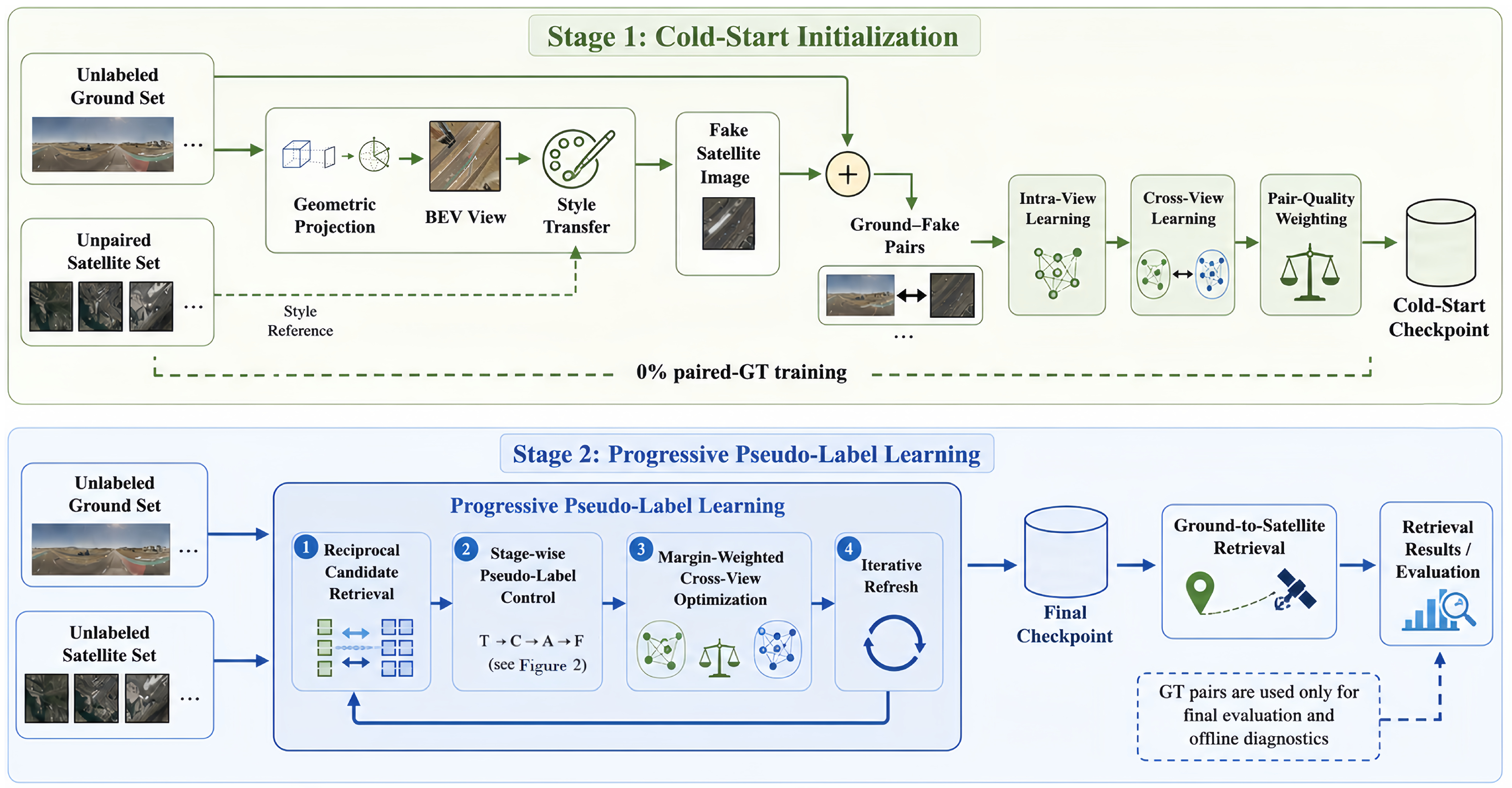
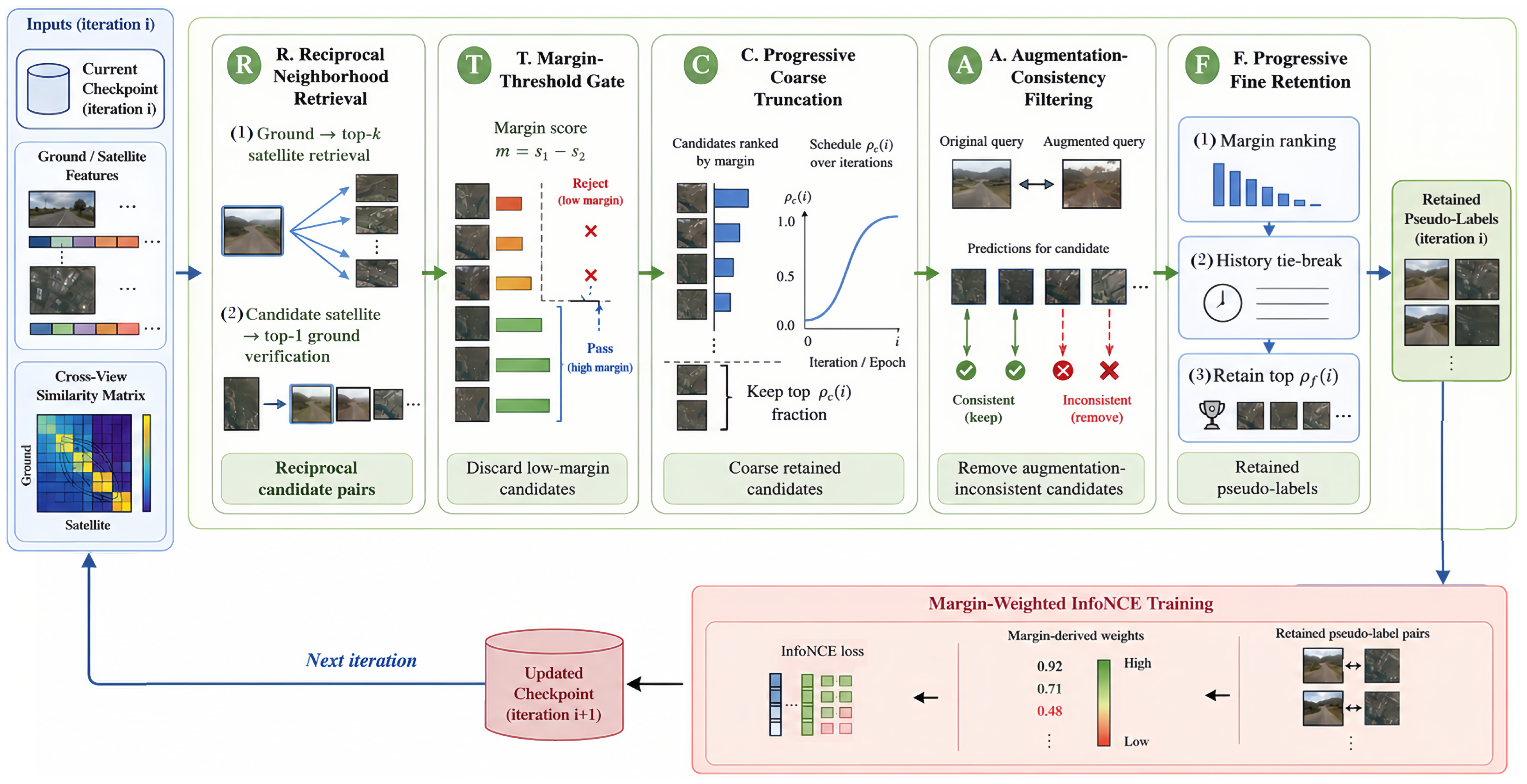
Figure 1 illustrates the overall PPLR training pipeline, whereas Figure 2 focuses on the iterative pseudo-label learning stage and details the retrieval, filtering, and update loop used after cold-start initialization. We structure PPLR as a two-stage unsupervised CVGL framework: an initial cold-start stage establishes cross-view feature alignment, followed by an iterative pseudo-label learning stage that alternates between generating pseudo-labels and updating the model. PPLR retains the ConvNeXt-Base/SAFA backbone and the geometric cold-start design, while adding lightweight pair-quality weighting and a structured pseudo-label selection pipeline.

Within the second stage, the pseudo-label generation pipeline uses three sequential control operations. First, reciprocal neighborhood retrieval expands the candidate pool beyond strict top-1 mutual matching. Second, margin-based coarse filtering controls pseudo-label quantity through an explicit progressive schedule. Third, consistency-guided fine filtering refines selection through augmentation consistency, margin-based ranking, and history stability. Lightweight training refinements, including margin-weighted loss and cold-start pair-quality weighting, further improve the pipeline. These operations provide functionally distinct controls within Stage 2, but are evaluated as a combined pipeline rather than as separable contributions [35].

The encoder/backbone remains ConvNeXt-Base, followed by Spatial-Aware Feature Aggregation (SAFA) [6], matching the baseline configuration.

4.2. Cold-Start Initialization

The cold-start stage comprises three steps. First, geometric projection generates synthetic satellite images from ground panoramas through viewpoint transformation that maps street-level perspective to aerial perspective; these synthetic images provide coarse geometric correspondence but lack realistic satellite texture. A generative adversarial network further refines the synthetic images toward realistic satellite appearances, bridging the visual gap between projected views and real satellite imagery. Second, intra-view contrastive learning separately learns modality-specific features for each view. Spatially augmented variants of the same image serve as positive pairs, while different images serve as negatives. This encourages the model to learn view-invariant representations within each modality. Third, ground-fake cross-view contrastive learning aligns the two modalities by treating each ground panorama and its corresponding refined fake satellite view as a positive pair. This step establishes initial cross-view semantic alignment without requiring any real paired ground-satellite correspondences. PPLR introduces a lightweight pair-quality weighting refinement to this third step.

For each ground–fake pair in an active minibatch, let $s_i^{+}$ denote the cosine similarity of the positive pair. The negative search is minibatch-local: $s_i^{-}$ is the maximum ground-to-fake cosine similarity among the other entries in the active minibatch, with the positive diagonal excluded. Equal maxima have the same similarity value and therefore produce the same margin and sample weight, irrespective of which tied index is returned. The pair-quality margin is defined as

$$q_i=s_i^{+}-s_i^{-}.$$

(1)

A larger $q_i$ indicates that the positive pair is more clearly separated from its hardest negative, which corresponds to higher pair quality. These margins are normalized batch-wise to $[0,1]$ and mapped to per-sample weights via a linear transform:

$$w_i=\gamma +\delta ·{\displaystyle \frac{q_i-{\min }_j{q}_j}{{\max }_j{q}_j-{\min }_j{q}_j+ϵ}},$$

(2)

where the fixed default is $(\gamma ,\delta )=(0.8,0.2)$. These weights serve as per-sample coefficients in the InfoNCE (information noise-contrastive estimation) loss, providing lightweight pair-quality weighting rather than a labeled quality estimator. This mechanism is applied only during cold-start initialization; the pseudo-label learning stage operates on real ground–satellite pairs where the coarse filtering handles quantity scheduling and the fine filtering handles quality assessment.

4.3. Reciprocal Neighborhood Retrieval

Figure 2 illustrates the PPLR progressive pseudo-label filtering pipeline. Ground and satellite features are extracted to form a cross-view similarity matrix. The pseudo-label engine performs reciprocal neighborhood retrieval, applies margin-based coarse filtering, and refines through consistency-guided fine filtering. Selected pseudo-labels drive weighted InfoNCE training, and the updated model feeds back into the next iteration.

In each training epoch, features are extracted for all N ground queries and N satellite images, denoted as $\mathbf{G}\in {\mathbb{R}}^{N\times d}$ and $\mathbf{S}\in {\mathbb{R}}^{N\times d}$, respectively. The similarity matrix is:

$$\mathbf{M}=\mathbf{G}{\mathbf{S}}^{\top }\in {\mathbb{R}}^{N\times N}.$$

(3)

Existing strict top-1 mutual matching requires the global top-1 satellite $\arg {\max }_j{M}_{ij}$ for each query to rank that query as its own top-1 ground match. This strict criterion can reject otherwise plausible candidates.

PPLR relaxes this to reciprocal neighborhood retrieval. For each query i, its top-k most similar satellite candidates ${\mathcal{C}}_i=\{j:M_{ij}\mathrm{is}\mathrm{in}\mathrm{t}\mathrm{o}\mathrm{p}\text{-}k\}$ are examined. Any candidate $j\in {\mathcal{C}}_i$ for which $i=\arg {\max }_{i^{\prime }}{M}_{i^{\prime }j}$ is retained, i.e., query i is the top-1 ground match for satellite j. Formally, the retrieved candidate set is:

$$\mathcal{E}=\{(i,j):j\in \mathrm{t}\mathrm{o}\mathrm{p}\text{-}k\left(M_{i,:}\right)\wedge i=\arg \underset{i^{\prime }}{\max }{M}_{i^{\prime }j}\}.$$

(4)

This mechanism expands the retrieved candidate pool compared with strict top-1 mutual matching while preserving reciprocal consistency. It is not the final pseudo-label selection: downstream coarse filtering and fine filtering still determine which candidates are ultimately retained. The candidate top-k is the main structural hyperparameter of this module; its sensitivity is analyzed in Section 5.7. The selected candidate for each query is the reciprocal match with the highest similarity to that query. If multiple satellites satisfy the reciprocal condition for the same query, the one with the highest similarity is chosen.

4.4. Margin-Based Coarse Filtering

After neighborhood retrieval, PPLR applies an explicit margin-based coarse filtering for quantity scheduling before the subsequent quality refinement. The coarse filtering combines a margin threshold and a progressive keep-ratio.

For each query i, let $j_i^{\left(1\right)}=\arg {\max }_j{M}_{ij}$ denote its globally most similar satellite candidate and $j_i^{\left(2\right)}=\arg {\max }_{j\ne j_i^{\left(1\right)}}{M}_{ij}$ denote the second-most similar candidate. The retrieval margin is:

$${\mathrm{margin}}_i=M_{i{j}_i^{\left(1\right)}}-M_{i{j}_i^{\left(2\right)}}.$$

(5)

This query-level retrieval margin measures top-1 versus top-2 separation across the full satellite gallery. It is used uniformly for queries that pass the retrieval stage, and should not be conflated with the cold-start pair-quality margin or a neighborhood-level separability statistic.

In the baseline threshold-relaxation approach, the global threshold decreases with epoch and more pseudo-labels naturally enter the training set. PPLR records the quantity schedule explicitly through a keep-ratio alongside the margin threshold, so the evaluated implementation exposes these two operating controls separately.

The coarse filtering comprises two complementary mechanisms. First, a margin threshold ${\theta }_t$ retains only candidates for which ${\mathrm{margin}}_i\ge {\theta }_t$. The threshold decays per epoch via a cosine schedule:

$${\theta }_t={\theta }_0·{\displaystyle \frac{1+\cos (\pi ·t/T)}{2}},$$

(6)

where ${\theta }_0$ is the initial threshold and T is the total number of training epochs. This threshold provides an initial coarse quality check. Second, after applying the margin threshold, the remaining candidates are sorted by their retrieval margin. Only the top fraction governed by the keep-ratio ${\rho }_t$ is retained for the subsequent fine filtering. The keep-ratio follows a power-adjusted ease-in schedule that transitions from a conservative starting value ${\rho }_{\mathrm{start}}$ to a permissive ending value ${\rho }_{\mathrm{end}}$ over the first phase of training. Let $T_{\mathrm{ease}}$ denote the duration of the ease-in phase and $r_{\mathrm{mid}}$ a design target for its midpoint. The keep-ratio at epoch t is

$${\rho }_t={\rho }_{\mathrm{start}}+({\rho }_{\mathrm{end}}-{\rho }_{\mathrm{start}})·\min \left\{{\left({\displaystyle \frac{t}{T_{\mathrm{ease}}}}\right)}^p,1\right\},$$

(7)

where the power p is determined analytically from ${\rho }_{\mathrm{start}}$, ${\rho }_{\mathrm{end}}$, and $r_{\mathrm{mid}}$ so that the schedule passes through the midpoint target. Once the normalized progress reaches unity, the keep-ratio is clipped to ${\rho }_{\mathrm{end}}$ and remains saturated for the remainder of training. The specific parameter values are provided in Section 5.2.

4.5. Consistency-Guided Fine Filtering

After coarse filtering controls quantity through the margin threshold and keep-ratio, PPLR applies consistency-guided fine filtering for quality refinement. The fine filtering follows a clear sequential structure. First, an augmentation consistency pre-filter removes unstable queries. Second, the remaining queries are ranked by their retrieval margin. Third, after epoch $t_h$, history stability provides a subordinate tie-break. Fourth, a progressive retention ratio retains the top fraction of ranked queries.

For each query that passes the margin threshold of coarse filtering, a lightweight consistency score is computed under two mild query augmentations. The augmentation applies brightness and contrast perturbation, and Gaussian noise. Instead of directly measuring feature cosine similarity, the score assesses retrieval prediction stability across the two augmented views. Let $\widehat{j}$ and ${\widehat{j}}^{\prime }$ denote the top-1 retrieved satellite candidates for the original and augmented query, respectively, and let g and $g^{\prime }$ denote the corresponding retrieval margins ${\mathrm{margin}}_i$. The consistency score is:

$$c_i=\alpha ·\mathbf{1}[\widehat{j}={\widehat{j}}^{\prime }]+(1-\alpha )·\left(1-{\displaystyle \frac{|g-g^{\prime }|}{\left|g\right|+|g^{\prime }|+ϵ}}\right),$$

(8)

where $ϵ={10}^{-6}$. The first term rewards cases in which the top-1 candidate remains unchanged; the second term measures how consistent the retrieval margin remains. The two terms are weighted by $\alpha$ and $1-\alpha$, respectively. Queries with consistency score below a threshold ${\tau }_c$ are discarded entirely and do not enter subsequent ranking. This is a hard instability pre-filter, not the primary ranking signal.

The retrieval margin defined in Equation (5) is the primary ranking signal. Within the fine filtering stage, the retained queries are ranked by ${\mathrm{margin}}_i$ in descending order. A larger ${\mathrm{margin}}_i$ indicates that the top-1 candidate of the query is more clearly separated from its global runner-up, and therefore higher reliability.

After a history activation epoch $t_h$, an exponentially decayed assignment stability signal is maintained for each query. A history record tracks pseudo-label assignments with a decay factor; the stability score is derived from the ratio of consistently repeated assignments to the total decayed count. This score is a subordinate tie-breaker when ${\mathrm{margin}}_i$ values are close. Its influence is intentionally minimized so that ranking is governed primarily by the retrieval margin; history stability provides only a late-stage refinement for ties that would otherwise be arbitrary.

The retention ratio controls what fraction of ranked queries are retained after fine filtering. To distinguish it from the coarse-stage keep-ratio ${\rho }_t$, this retention ratio is used only within the fine filtering stage after consistency pre-filtering and margin-based ranking. It follows a progressive schedule that starts from a conservative value and increases toward full retention via a cosine ease-in schedule. In early epochs, the consistency pre-filter already removes a large fraction of low-quality queries. The retention ratio provides additional conservative pruning. In later epochs, as the retention ratio saturates at its final value, its direct effect diminishes. The primary quality control then shifts to the consistency pre-filter and margin-based ranking. The retention ratio is therefore a progressively relaxing quality-control layer alongside the coarse filtering keep-ratio.

4.6. Weighted InfoNCE and Model Update

Once pseudo-labels are selected through the Stage 2 filtering pipeline, the model is updated via weighted InfoNCE training. Existing pipelines use a binary mask in InfoNCE loss, giving all pseudo-label samples equal weight. Pseudo-label selection via the coarse filtering and fine filtering remains the primary supervisory mechanism.

For each query ultimately retained for training, its retrieval margin is min–max normalized within the retained batch and mapped to a per-sample weight. The mapping is designed to produce only marginal variation across samples, so the loss weighting remains a lightweight refinement. These weights scale the per-sample terms in the InfoNCE loss, yielding a weighted mean:

$$\mathcal{L}={\displaystyle \frac{{\sum }_i{w}_i·{\mathcal{l}}_i}{{\sum }_i{w}_i+ϵ}},$$

(9)

where ${\mathcal{l}}_i$ is the per-sample InfoNCE loss, $w_i$ is the normalized margin-derived weight, and $ϵ={10}^{-12}$.

Algorithm 1 summarizes the complete PPLR pseudo-label learning procedure. The pipeline iterates over training epochs: feature extraction, similarity computation, reciprocal neighborhood retrieval, margin-based coarse filtering, consistency-guided fine filtering, and margin-weighted InfoNCE update.

Algorithm 1 PPLR Pseudo-Label Learning

Input: Cold-start model ${\theta }^{\left(0\right)}$, ground images $\mathcal{G}$, satellite images $\mathcal{S}$ Parameters: candidate top-k, consistency threshold ${\tau }_c$, history epoch $t_h$, total epochs E, initial margin threshold ${\theta }_0$ Output: Trained model ${\theta }^{\left(E\right)}$ for $t=0$ to $E-1$ do    1. Extract features: $\mathbf{G}\leftarrow f_{\theta }\left(\mathcal{G}\right)$, $\mathbf{S}\leftarrow f_{\theta }\left(\mathcal{S}\right)$    2. Similarity: $\mathbf{M}\leftarrow \mathbf{G}{\mathbf{S}}^{\top }$    3. Reciprocal neighborhood retrieval (Equation (4))    4. Margin-based coarse filtering (Equation (7)):        a. Hard margin threshold: retain candidates with ${\mathrm{margin}}_i\ge {\theta }_t$        b. Soft truncation: keep top ${\rho }_t$ fraction by retrieval margin    5. Consistency-guided fine filtering:      a. Augmentation consistency pre-filter (threshold ${\tau }_c$, hard instability removal)        b. Rank by retrieval margin ${\mathrm{margin}}_i$ (primary signal)        c. History stability ($t\ge t_h$, subordinate tie-break)        d. Retention-ratio control (progressive cosine ease-in)    6. Margin-weighted InfoNCE (Equation (9))    7. Update $\theta$ via gradient descent on $\mathcal{L}$ end for return  ${\theta }_E$

5. Results

5.1. Datasets and Metrics

We evaluate on two standard benchmarks for cross-view geo-localization:

The CVUSA dataset [1,2] contains ground-level panoramas and corresponding satellite images across the United States, with approximately 35,532 training pairs and 8884 test pairs.

The CVACT dataset [63] provides a complementary evaluation benchmark with a different collection setting. It contains approximately 35,532 training pairs, 8884 validation pairs (CVACT Val), and a larger test set (CVACT Test) of 92,802 pairs densely sampled from Canberra, Australia. Unless explicitly stated as “CVACT Test,” the term “CVACT” hereafter refers to the validation split (CVACT Val), which is the primary evaluation split for this dataset in the reported literature. Both datasets are used under the 0% GT (fully unsupervised) protocol, where no ground-truth cross-view correspondences are used during training.

Metrics. Following standard practice, we report Recall@1 (R@1), Recall@5 (R@5), Recall@10 (R@10), and Recall@top-1% (R@1%). R@1 is the primary metric. R@1% uses the floor of 1% of the gallery size, and exact ties receive the minimum rank. All reported differences are in percentage points (pp). In addition to within-dataset evaluation and source-only cross-dataset transfer experiments, we conduct ablation studies, hyperparameter sensitivity analyses, and mechanism diagnostics.

5.2. Implementation Details

We adopt the ConvNeXt-Base [64] + SAFA [6] dual-branch backbone, following the reported base configuration. The image size is $384\times 384$ for both ground and satellite views. The optimizer is AdamW with a learning rate of ${10}^{-4}$. The learning rate schedule is cosine annealing [65]. The batch size is 128 for both cold-start and second-stage training. The second stage trains for 40 epochs. The neighborhood size is $k=5$ for both CVUSA and CVACT. Cold-start training consists of 12 epochs of intra-view contrastive learning followed by 28 epochs of ground–fake cross-view training. All headline and table values use the pre-specified final checkpoint after the 40-epoch run. A highest-R@1 epoch, when reported, is a retrospective diagnostic after training and is not used for model selection, early stopping, or labeled checkpoint selection. Ground truth is joined only after the candidate set is frozen for offline precision and rank diagnostics. The verified implementation environment used Python (v3.9.7) with PyTorch (v2.7.0+cu128) and CUDA (v12.8) on an NVIDIA RTX PRO 6000 Blackwell Server Edition GPU (NVIDIA Corporation, Santa Clara, CA, USA).

Key hyperparameters. The cold-start pair-quality weighting uses batch-wise min–max normalization. The coarse-filtering margin threshold decays from ${\theta }_0=0.05$ (CVUSA) or $0.025$ (CVACT) via cosine schedule. The fine-stage retention ratio increases from $0.50$ to $1.00$ via cosine ease-in over the initial training phase. The coarse-filtering keep-ratio starts at $0.30$ and reaches $1.00$ following the power-adjusted ease-in schedule (Equation (7)). The consistency pre-filter threshold is ${\tau }_c=0.60$, with the consistency score weighted by $\alpha =0.7$ toward candidate stability and $1-\alpha =0.3$ toward margin consistency. History stability activates after epoch $t_h=15$. The cold-start pair-quality weighting maps pair margins to per-sample weights in $[0.8,1.0]$. These defaults are fixed without consulting labeled validation accuracy or offline pseudo-label precision; sensitivity results evaluate robustness within the tested range rather than automatic parameter selection.

The UCVGL comparison uses the Base configuration: ConvNeXt-Base, SAFA aggregation, and $384\times 384$ inputs. UCVGL-Small uses ConvNeXt-Small and $224\times 224$ inputs; both configurations use separate view encoders and SAFA aggregation. The Base descriptor is 8192-dimensional and has 175,468,160 parameters. PPLR also uses ConvNeXt-Base, SAFA, and $384\times 384$ inputs, so UCVGL-Base is the closest scale-matched comparator.

The table makes the comparison boundary explicit. UCVGL-Base and PPLR use the same CVUSA/CVACT ground–satellite direction and 0% paired-GT setting, so their in-domain rows and source-only transfer rows can be compared directly. Dynamic-threshold CVGL is included because its confidence schedule addresses a related pseudo-label selection problem, but its 1–100% paired-GT protocol is semi-supervised and is not directly comparable to PPLR’s 0% setting. The remaining methods use drone–satellite benchmarks and/or different target-domain optimization procedures; their reported numbers provide related-work context but are not inserted into the same numerical ranking. A released unpaired drone–satellite formulation can be diagnostically transferred, but that exercise does not measure its native performance.

The verified encoder and input-scale configurations are summarized in

Table 2. UCVGL scale clarification. UCVGL-Base is the closest same-scale comparator for PPLR; only configuration fields verified from the cited implementation are shown.

Property	UCVGL-Small	UCVGL-Base
Backbone	ConvNeXt-Small	ConvNeXt-Base
Input resolution	$224\times 224$	$384\times 384$
Aggregation	SAFA	SAFA

.

5.3. Comparison with Existing Methods

Table 3. Benchmark context on CVUSA, CVACT Val, and CVACT Test. The GT column records the supervision protocol; rows with different supervision are not treated as same-protocol alternatives. Bold and underlined values denote the highest and second-highest result in each metric column, respectively. Gray shading marks methods for which every reported R@1, R@5, and R@10 value is lower than the corresponding PPLR value; R@1% is not used for the shading criterion. ^† Polar Transform. ^‡ Without Hard Negative Sampling. ^★ Frozen geometric foundation model features. UCVGL-Base denotes the scale-matched ConvNeXt-Base/$384\times 384$ configuration.

Method	GT	CVUSA				CVACT Val				CVACT Test
		R@1	R@5	R@10	R@1%	R@1	R@5	R@10	R@1%	R@1	R@5	R@10	R@1%
CVM-Net [5]	100%	22.47	49.98	63.18	93.62	20.15	45.00	56.87	87.57	5.41	14.79	25.63	54.53
Liu [63]	100%	40.79	66.82	76.36	96.12	46.96	68.28	75.48	92.01	19.21	35.97	43.30	60.69
SAFA [6]	100%	81.15	94.23	96.85	99.49	78.28	91.60	93.79	98.15	—	—	—	—
SAFA † [6]	100%	89.84	96.93	98.14	99.64	81.03	92.80	94.84	98.17	—	—	—	—
DSM † [32]	100%	91.96	97.50	98.54	99.67	82.49	92.44	93.99	97.32	—	—	—	—
L2LTR [22]	100%	91.99	97.68	98.65	99.75	83.14	93.84	95.51	98.40	58.33	84.23	88.60	95.83
UCVGL-Small [8]	100%	93.53	98.42	99.18	99.77	84.44	94.85	96.15	98.53	57.71	86.35	90.40	98.49
GeoDTR [20]	100%	93.76	98.47	99.22	99.85	85.43	94.81	96.11	98.26	62.96	87.35	90.70	98.61
TransGeo [4]	100%	94.08	98.36	99.04	99.77	84.95	94.14	95.78	98.37	—	—	—	—
Sample4Geo ‡ [3]	100%	97.83	99.63	99.75	99.89	87.49	96.56	97.50	98.98	60.57	89.50	92.99	98.92
MFRGN [24]	100%	98.24	99.56	99.72	99.88	88.87	96.67	97.48	98.99	—	—	—	—
PanoBEV [23]	100%	98.71	99.70	99.78	99.86	91.90	97.23	97.84	98.84	73.68	93.53	95.11	98.81
${\mathrm{Geo}}^2$ ★ [26]	100%	98.83	99.72	99.79	99.91	94.36	97.41	97.97	99.05	75.08	94.89	95.77	99.01
GenGeo [27]	100%	98.94	99.73	99.82	99.91	90.63	96.52	97.33	98.55	71.92	92.53	94.40	98.67
UCVGL-Small [8]	0%	87.90	95.86	97.51	99.63	82.96	92.96	94.43	97.37	58.85	84.27	88.16	97.45
UCVGL-Base [8]	0%	91.04	97.05	98.23	99.63	84.58	93.95	95.29	97.59	60.53	86.35	89.77	97.52
PPLR (Ours)	0%	96.30	98.98	99.48	99.80	89.23	96.13	96.86	98.45	66.84	90.77	93.17	98.32

retains the original benchmark context on CVUSA, CVACT Val, and CVACT Test. The GT column makes the supervision difference explicit; only the 0% paired-ground-truth UCVGL-Base row is used as the primary same-scale comparator. Methods with different supervision or native protocols are contextual references rather than a directly comparable ranking.

The 0% GT comparison gives PPLR R@1 gains of +5.26 pp on CVUSA Test, +4.65 pp on CVACT Val, and +6.31 pp on CVACT Test over UCVGL-Base. PPLR also remains higher than UCVGL-Base at R@5, R@10, and R@1% on all three splits. CVACT Test is consistently harder than CVACT Val for both methods, so the held-out Test result provides a stricter check of the same unsupervised protocol. These values use the same ConvNeXt-Base + SAFA scale and evaluation direction; optimization and training schedules are not claimed to be identical across methods.

The comparison separates two effects that are easy to conflate. First, the matched-scale UCVGL-Base row provides a controlled reference for the 0% paired-ground-truth setting. Second, the supervised rows show the broader benchmark range but use paired annotations and therefore cannot be interpreted as a direct test of the unsupervised claim. Within the matched rows, PPLR’s gains are consistent across the three splits, while the lower CVACT Test scores indicate that the held-out test protocol remains more difficult than CVACT Val.

5.4. Source-Only Cross-Dataset Transfer

We evaluate source-only transfer in three directions: CVUSA → CVACT Val, CVUSA → CVACT Test, and CVACT → CVUSA Test. The source-trained checkpoint is evaluated directly on the target split without target-domain optimization.

Table 4. Source-only cross-dataset transfer. The GT column gives the paired ground truth used in the source dataset; no target-domain optimization is performed. Bold and underlined values denote the highest and second-highest result in each metric column, respectively. Gray shading marks methods for which every reported R@1, R@5, and R@10 value is lower than the corresponding PPLR value; R@1% is not used for the shading criterion. Results with different GT ratios are contextual because the source-supervision protocols differ. ^† Polar transformation. ^★ Frozen geometric foundation-model features. MFRGN+ uses pro-cropping and hard negative sampling.

Method	GT	CVUSA → CVACT Val				CVUSA → CVACT Test				CVACT → CVUSA
		R@1	R@5	R@10	R@1%	R@1	R@5	R@10	R@1%	R@1	R@5	R@10	R@1%
SAFA [6]	100%	30.40	52.93	62.29	85.82	—	—	—	—	21.45	36.55	43.79	69.83
DSM † [32]	100%	33.66	52.17	59.74	79.67	—	—	—	—	18.47	34.46	42.28	69.01
TransGeo [4]	100%	37.81	61.57	69.86	89.14	—	—	—	—	17.45	32.49	40.48	69.14
GeoDTR [20]	100%	43.72	66.99	74.61	91.83	11.24	18.69	23.67	72.09	29.85	49.25	57.11	82.47
MFRGN [24]	100%	51.61	73.91	80.55	94.24	—	—	—	—	49.12	70.29	77.41	95.16
L2LTR † [22]	100%	52.58	75.81	77.39	93.51	—	—	—	—	33.00	51.87	60.63	84.79
Sample4Geo [3]	100%	56.62	77.79	87.02	94.69	27.78	52.08	60.33	94.88	44.95	64.36	72.10	90.65
GeoDTR+ [21]	100%	60.16	79.97	84.67	94.48	—	—	—	—	52.56	73.08	79.82	94.80
${\mathrm{Geo}}^2$ ★ [26]	100%	63.17	82.53	87.88	95.09	—	—	—	—	55.14	73.58	80.03	95.33
PanoBEV [23]	100%	67.79	84.06	87.96	95.05	44.10	70.68	75.86	95.31	—	—	—	—
GenGeo [27]	100%	71.27	87.34	90.79	96.69	—	—	—	—	55.66	74.04	80.26	94.78
MFRGN+ [24]	100%	79.12	91.09	93.17	96.79	—	—	—	—	69.28	84.91	89.60	97.69
MRGeo [29]	100%	82.73	93.21	—	97.92	—	—	—	—	47.73	65.65	—	90.85
UCVGL-Base [8]	0%	68.65	84.89	88.43	95.49	38.97	65.04	72.03	94.92	53.67	72.87	78.93	93.17
PPLR (Ours)	0%	73.06	89.05	91.99	97.06	41.35	70.10	77.16	96.81	58.79	77.01	83.08	95.38

includes published baselines with their source paired-GT ratios and retains UCVGL-Base and PPLR under the 0% paired-ground-truth protocol. Results with different GT ratios provide protocol context rather than a single same-protocol ranking.

Within the matched 0% paired-ground-truth protocol, PPLR reaches R@1 of 73.06, 41.35, and 58.79 in the three directions, compared with 68.65, 38.97, and 53.67 for UCVGL-Base. These correspond to improvements of 4.41, 2.38, and 5.12 percentage points, respectively. The 100% GT rows span a broad range and include stronger results in the first and third directions, while PanoBEV records the highest R@1 on CVUSA → CVACT Test (44.10 versus 41.35 for PPLR). These observations are descriptive because those methods use source paired ground truth. The direction-dependent results and the remaining gap to the strongest 100% GT entries support partial transferability rather than domain invariance. They should be interpreted as source-only transfer, not target-domain adaptation.

5.5. Ablation Study

Table 5. Grouped and fine-grained ablations. (R): reciprocal neighborhood retrieval; (T): margin-threshold gate; (C): progressive coarse truncation; (A): augmentation-consistency filtering; (F): progressive fine retention. Grouped rows remove a complete control group, whereas fine-grained rows remove one listed operation while retaining the other operations. A checkmark indicates that an operation is retained and a cross indicates that it is removed; bold values identify the Full PPLR reference result.

Granularity	Variant	R	T	C	A	F	CVUSA R@1	CVACT R@1
Full	Full PPLR	✔	✔	✔	✔	✔	96.30	89.23
Grouped	w/o reciprocal retrieval	×	✔	✔	✔	✔	90.30	87.51
Grouped	w/o coarse control group	✔	×	×	✔	✔	37.55	77.71
Grouped	w/o fine control group	✔	✔	✔	×	×	74.61	87.56
Fine-grained	w/o margin-threshold gate	✔	×	✔	✔	✔	93.15	88.65
Fine-grained	w/o progressive coarse truncation	✔	✔	×	✔	✔	92.53	88.17
Fine-grained	w/o augmentation consistency	✔	✔	✔	×	✔	94.30	88.70
Fine-grained	w/o progressive fine retention	✔	✔	✔	✔	×	94.06	88.73

separates grouped control-group removals from fine-grained one-factor variants. The Full row uses the PPLR configuration; the ablation variants retain the provenance of their controlled runs. These rows are not a complete factorial design.

The grouped rows measure control-group removal, while the fine-grained rows measure the marginal change of one operation while the remaining controls stay active. The grouped coarse and fine control-group removals therefore need not equal the sum of individual fine-grained changes. The results support complementary and partially compensating controls within the evaluated configuration; they do not establish a complete factorial interaction or statistical significance.

The dataset dependence of the grouped rows is also informative but bounded. Removing the coarse control group produces the largest CVUSA degradation (96.30 to 37.55), whereas the corresponding CVACT decrease is smaller (89.23 to 77.71). Conversely, removing the fine control group changes CVUSA more than CVACT in this table. These differences describe the tested datasets and checkpoints; they are not evidence that a component is universally more important, and the fine-grained drops must not be added to recover a total module contribution.

5.6. Pseudo-Label Dynamics

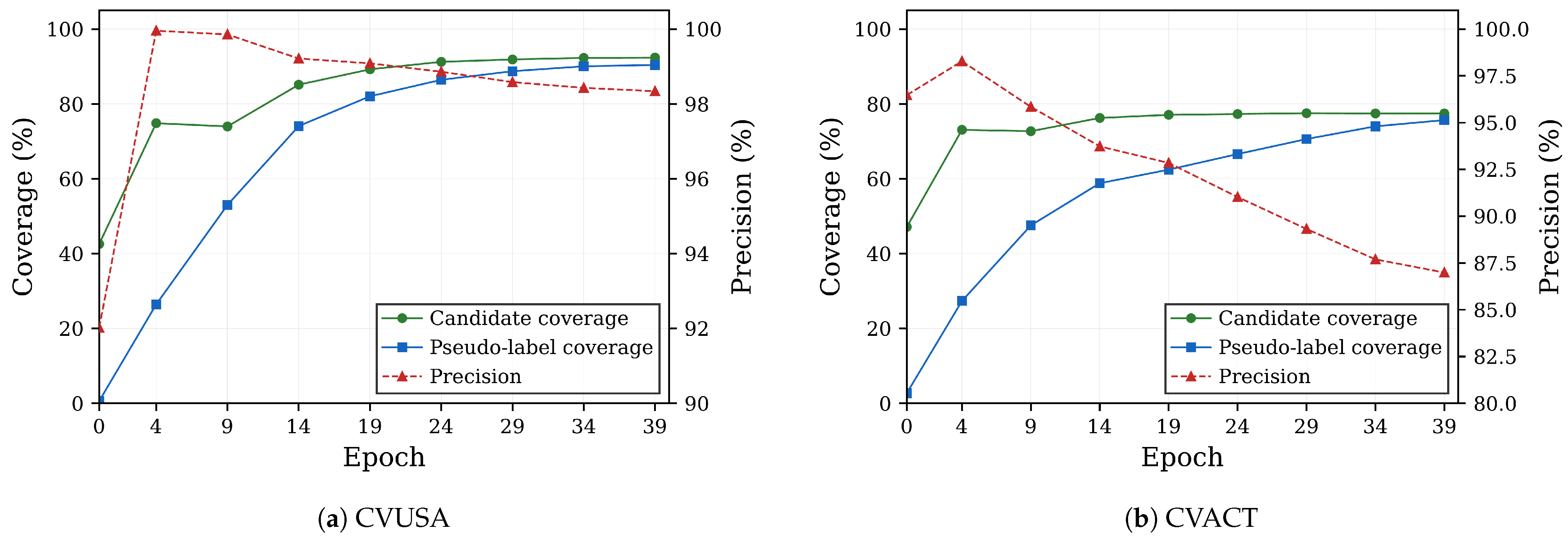
Figure 3 retains the original epoch-wise trajectory context for pseudo-label coverage and precision. The epoch-wise filtering trace is first reported in

Table 6. Pseudo-Label Filtering Dynamics at Key Epochs ($k=5$). Neighborhood Retrieval: Queries with at Least One Reciprocal Match. After Fine Filtering: Queries Surviving Consistency-guided Fine Filtering. Retention Ratio: Fraction of Retrieved Queries Retained for Training.

Epoch	CVUSA			CVACT
	RecNei	AfterFine	Retention Ratio (%)	RecNei	AfterFine	Retention Ratio (%)
0	15,120	213	1.41	16,744	964	5.76
5	27,917	11,512	41.24	26,272	11,033	42.00
10	26,256	21,676	82.56	26,322	19,131	72.68
15	30,486	26,891	88.21	27,196	21,197	77.94
20	31,836	29,337	92.15	27,316	22,500	82.37
25	32,491	30,968	95.31	27,521	23,992	87.18
30	32,708	31,663	96.81	27,540	25,361	92.09
35	32,804	32,022	97.62	27,532	26,502	96.26
39	32,828	32,127	97.86	27,526	26,889	97.69

, while the canonical operation-wise selection statistics used for the revised interpretation are reported separately in Figure 4 and

Table 7. Operation-wise selection statistics within Stage 2. Counts and percentages are reported for the final recorded selection; “-” indicates that retention is not defined before the first filtering operation.

Stage 2 Operation	Count	Coverage (%)	Precision (%)	Retention (%)	Diagnostic Role
Reciprocal retrieval	16,745	47.13	57.99	-	candidate expansion
Margin-threshold gate	6429	18.09	83.75	38.39	coarse quality gate
Progressive coarse truncation	1929	5.43	94.87	30.00	quantity control
Augmentation consistency	1929	5.43	94.87	100.00	stability check
Progressive fine retention	965	2.72	96.48	50.03	final retention

; the latter freezes candidate sets before joining ground truth for offline precision calculation.

The two trajectories show why coverage and precision should be read together. Early epochs admit only a small, conservative set, whereas later epochs expand the candidate pool and gradually increase the number of retained pairs. The CVACT curve reaches a larger initial coverage and follows a different precision trajectory, while CVUSA gains coverage more steadily. These curves motivate the separate operation-wise analysis below; they are not used to select a checkpoint using ground truth.

Table 6 retains the epoch-wise filtering trace underlying Figure 3 for $k=5$. The revised operation-level count, coverage, precision, and retention evidence is reported in Table 7.

The key-epoch table makes the trajectory interpretation concrete: both datasets move from a small, highly selective retained set toward broad coverage, but CVACT remains more conservative after fine filtering at the intermediate epochs. The final rows describe the curriculum trace and are not an additional source of headline performance values.

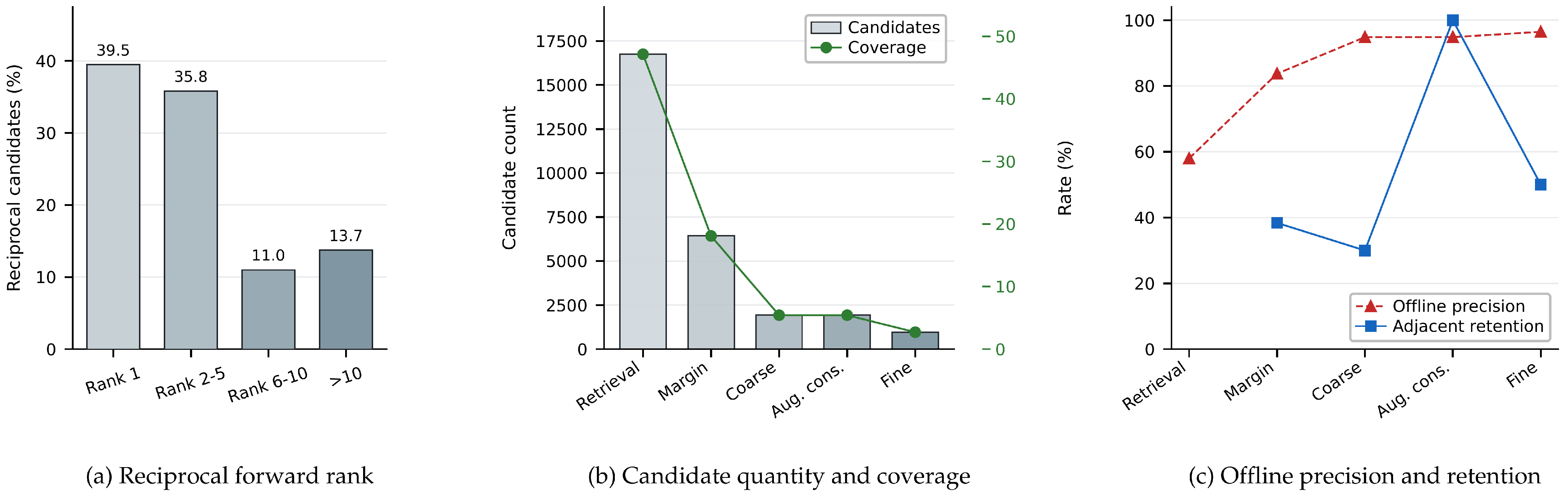
The mechanism plot complements the epoch trace by showing where the quantity–quality trade-off is resolved within an iteration. In Figure 4a, the four bars are the proportions of the 35,532 CVACT training locations whose reciprocal satellite candidate appears at forward ranks 1, 2–5, 6–10, or above 10; the tail shows why a strict top-1 rule would discard a non-trivial candidate pool. Figure 4b is read from left to right: bars give the nested candidate counts after raw reciprocal retrieval, the threshold gate, coarse truncation, consistency check, and fine retention, while the green line gives their coverage relative to the 35,532-location denominator. Figure 4c reports two different rates on the same nested snapshots: red triangles are offline precision after joining frozen selections with ground truth, and blue squares are adjacent retention relative to the preceding snapshot. Thus, the plot describes quantity reduction and post hoc quality together; it does not isolate a causal contribution for any one operation.

The operation-wise counts show the intended quantity–quality regulation within Stage 2. Reciprocal retrieval admits 16,745 candidates (47.13% coverage), after which the margin gate and progressive truncation reduce the set to 1929 candidates while the offline precision diagnostic rises from 57.99% to 94.87%. Augmentation consistency leaves this recorded count unchanged, and progressive fine retention produces the final 965-query set with 96.48% offline precision. These are descriptive diagnostics of frozen candidate sets; they do not isolate a causal effect for any single operation.

5.7. Sensitivity to Candidate Top-k

We evaluated the sensitivity of PPLR to the neighborhood size k while keeping the other settings fixed. The reporting schedule and retention sensitivity are summarized first in

Table 8. Hyperparameter and schedule sensitivity on CVACT Val. The table reports robustness within the evaluated settings; it does not establish an optimum or automatic parameter rule.

Factor	Setting/Variant	CVACT Val R@1
Cold-start weighting	$(\gamma ,\delta )=(1.0,0.0)$	88.81
Cold-start weighting	$(\gamma ,\delta )=(0.8,0.2)$, default	89.23
Cold-start weighting	$(\gamma ,\delta )=(0.6,0.4)$	89.13
Threshold schedule	linear	89.05
Threshold schedule	constant	88.72
Coarse retention	$0.2\to 1.0$	88.89
Coarse retention	$1.0\to 1.0$	88.17
Fine retention	$0.3\to 1.0$	88.98
Fine retention	$1.0\to 1.0$	88.73

; the top-k sweep then reports the R@1 diagnostic for $k\in \{1,3,5,7,10\}$ in

Table 9. Top-k sensitivity on CVUSA and CVACT Val across the completed five-setting sweep.

Neighborhood Size k	CVUSA R@1	CVACT Val R@1
1	95.57	88.86
3	95.50	88.67
5	96.30	89.23
7	96.02	88.80
10	95.82	89.04

. The values are 95.57, 95.50, 96.30, 96.02, and 95.82 on CVUSA, and 88.86, 88.67, 89.23, 88.80, and 89.04 on CVACT Val, respectively. The sweep is kept separate from the reporting schedule and weighting endpoints; it describes the observed neighborhood-size behavior and does not establish an optimum or an automatic unlabeled parameter-selection rule.

The sensitivity values remain within a compact band around the default, with the largest decrease occurring when the coarse retention curriculum is removed. This pattern is consistent with the interpretation that the settings regulate curriculum pace and selectivity; it does not show that every parameter is individually indispensable or that the default was selected using labeled validation accuracy.

The separate top-k table makes the tested $k=5$ setting explicit and keeps neighborhood-size sensitivity distinct from the weighting and retention schedules. Across the five tested values, the CVUSA range is 95.50–96.30 and the CVACT Val range is 88.67–89.23; the fixed $k=5$ configuration lies at the upper end of both tested ranges. The evaluated neighborhood sizes therefore give a relatively narrow sensitivity band. The fixed $k=5$ setting is used consistently in the experiments; these diagnostic values are not used for parameter selection, and no automatic unlabeled selection rule is claimed.

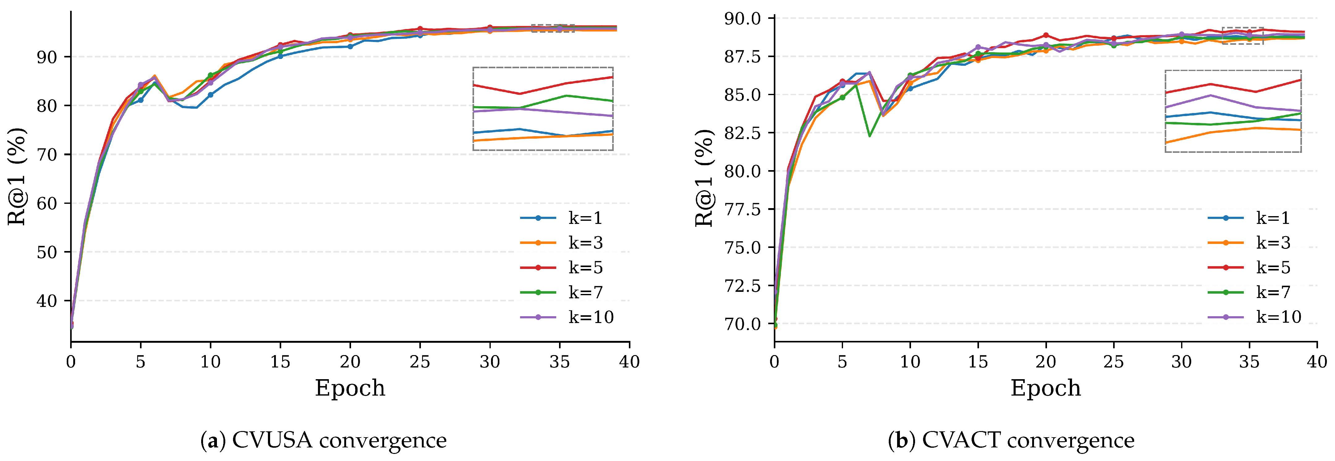
Figure 5 retains the completed convergence traces for the five neighborhood sizes. The curves follow similar trajectories on both datasets, and the late-epoch insets show that their endpoint separation is small relative to the common convergence pattern. The traces provide robustness context for Table 9; they describe convergence behavior rather than determine the reported result.

5.8. Multi-Seed Stability Validation

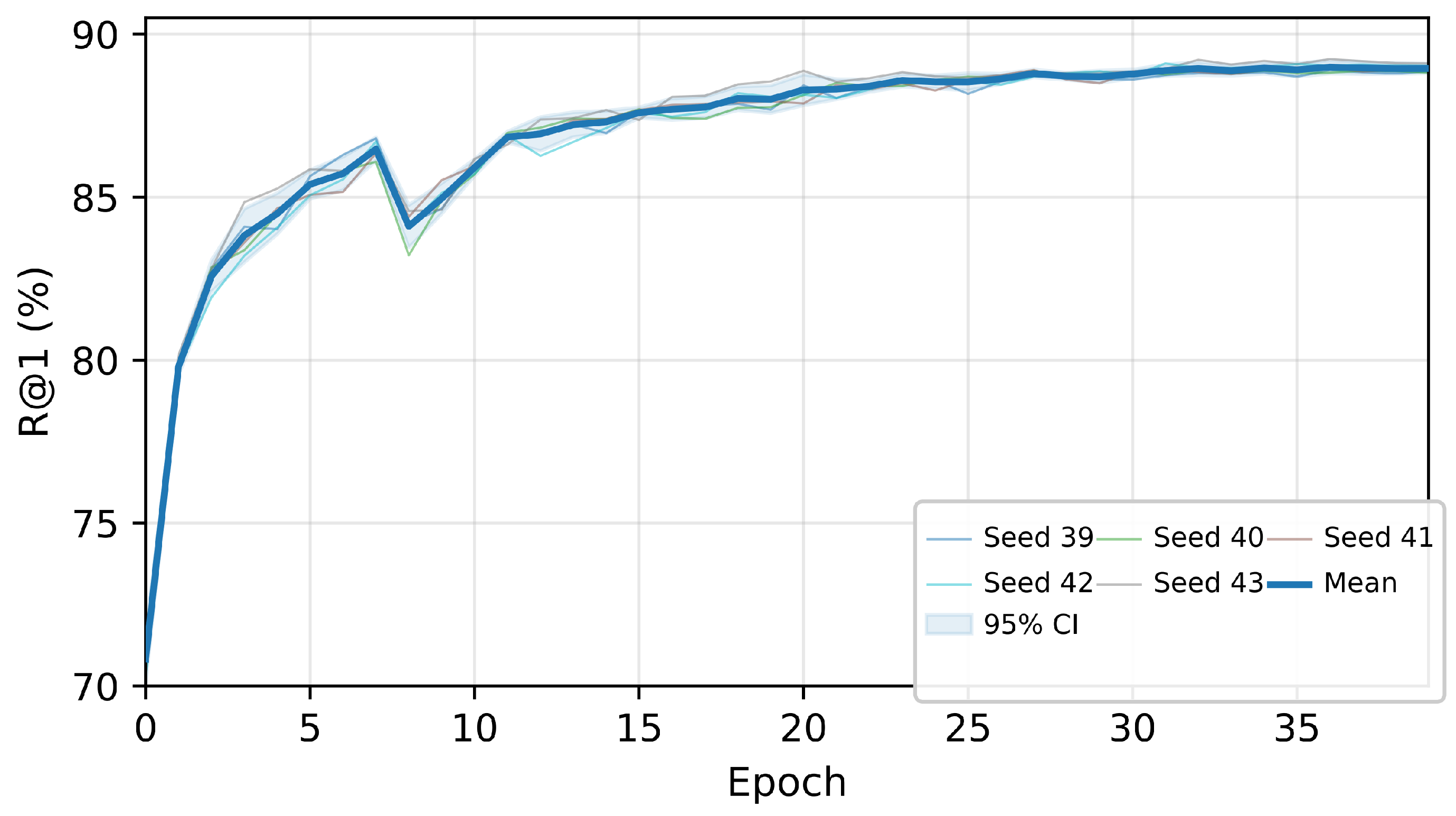
Pseudo-label learning is stochastic due to random initialization, data augmentation, and batch sampling. We therefore evaluated the CVACT Val configuration with five seeds (39, 40, 41, 42, and 43).

Table 10. Multi-seed stability on CVACT Val.

Seed	Best R@1	Best Epoch	Last R@1
39	88.90	36	88.86
40	88.89	32	88.82
41	88.96	36	88.94
42	89.24	36	89.10
43	89.10	31	89.03
Mean ± Std	89.02 ± 0.15	34.2	88.95 ± 0.12

reports the R@1 trajectory endpoints for each seed. The retrospective peak R@1 varies from 88.89 to 89.24, with a mean of 89.02 and a standard deviation of 0.15 percentage points. The run-end R@1 has mean 88.95 and standard deviation 0.12. These values describe run stability.

The endpoint values span 0.28 percentage points (88.82–89.10), with a standard deviation of 0.12 percentage points. Figure 6 visualizes the corresponding mean convergence trajectory and its descriptive 95% confidence interval. The interval is included to show run-to-run dispersion for these five seeds and is not used as a statistical significance test.

5.9. Qualitative Retrieval and Diagnostic Feature Analysis

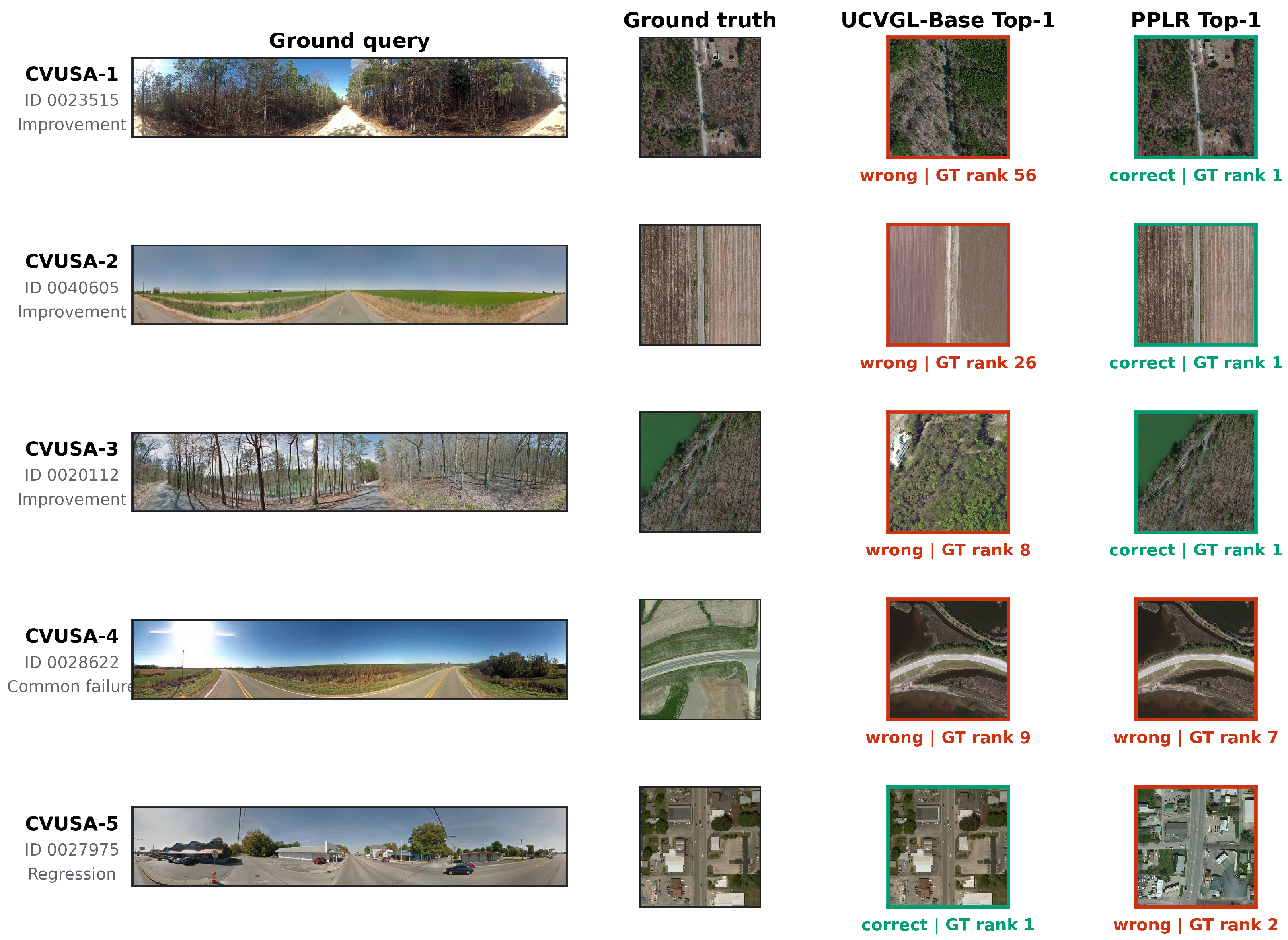
Figure 7 shows five CVUSA cases: three improvements, one common failure, and one regression. The examples illustrate retrieval behavior rather than estimate a population-level success rate; aggregate CVACT conclusions are based on the complete benchmark metrics and the operation-wise diagnostics reported above.

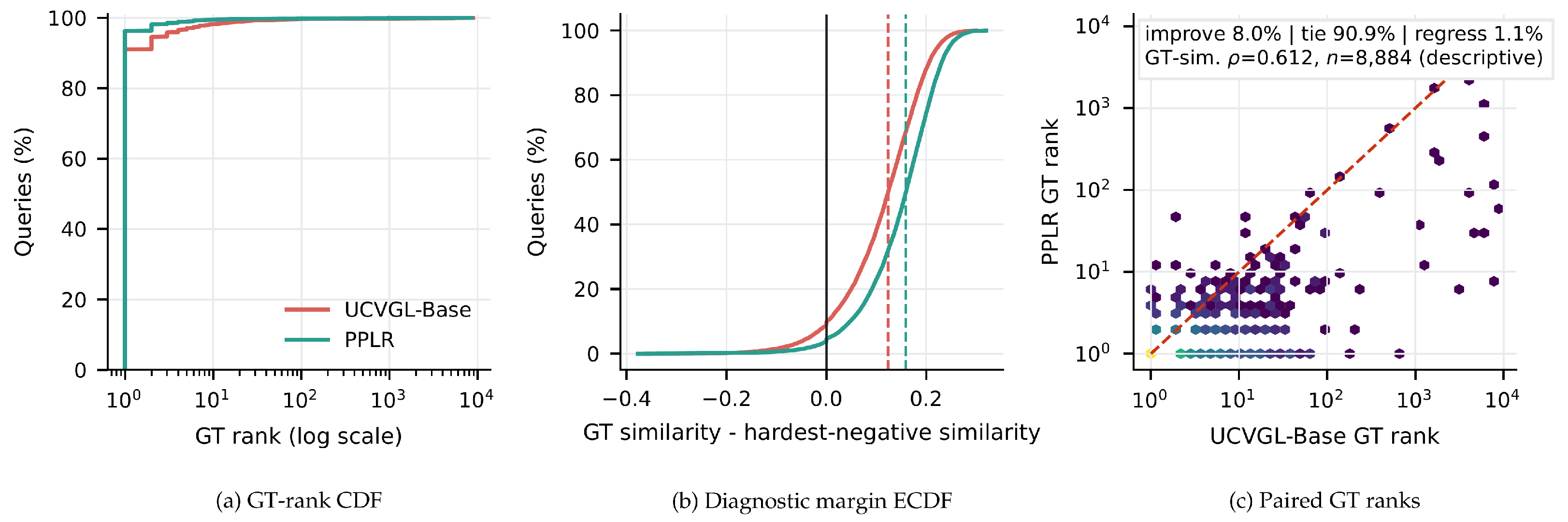
Figure 8 summarizes CVUSA retrieval behavior using GT-rank distributions, diagnostic query-level margins, and paired ranks. The descriptive Spearman association between matched GT-positive similarities is $\rho =0.6117$ over $n=8884$ valid query/ground-truth pairs.

The retrieval-behavior panels show how the aggregate gain is distributed across queries. In Figure 8a, the PPLR curve rises faster at small ranks, indicating more queries with an early ground-truth match. In Figure 8b, the PPLR median margin is shifted to the right, although the curves overlap and therefore do not imply universal improvement. In Figure 8c, the annotation records 8.0% improved ranks, 90.9% ties, and 1.1% regressions under the paired rank convention; the diagonal is only a visual reference. The Spearman value is descriptive and measures agreement between the two methods’ matched GT-positive similarities, so it does not identify a causal mechanism or a stage-interaction effect.

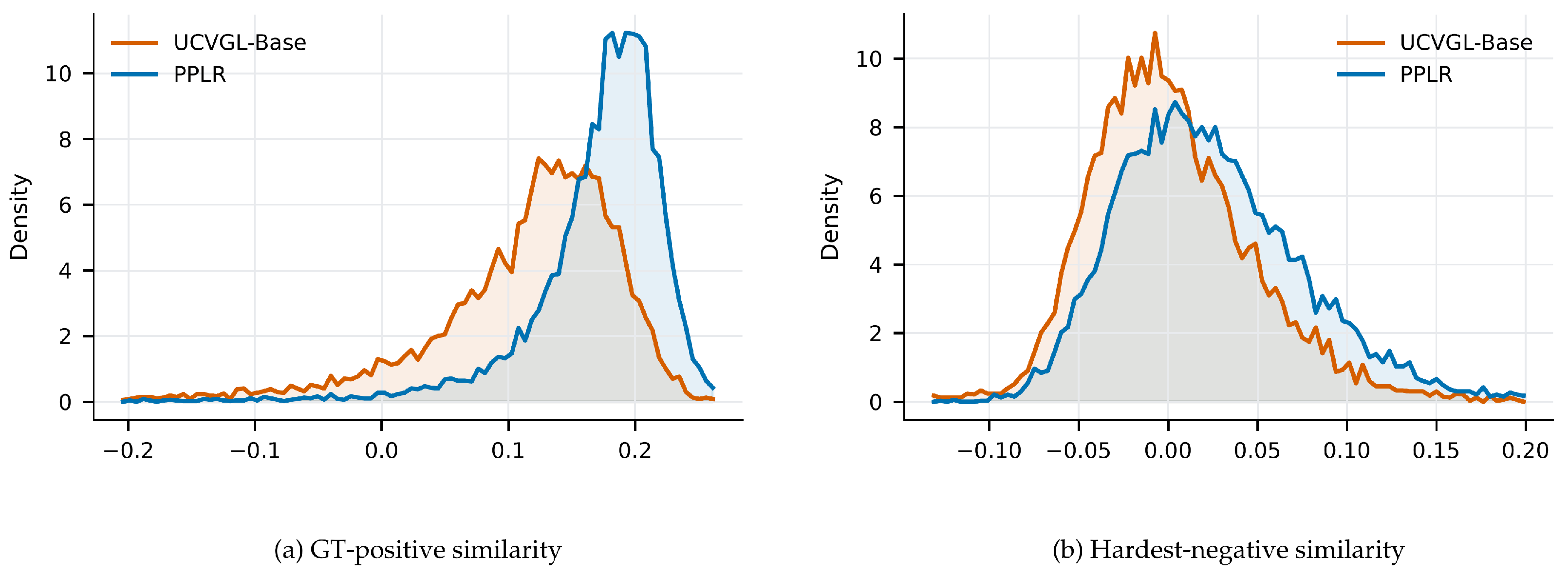
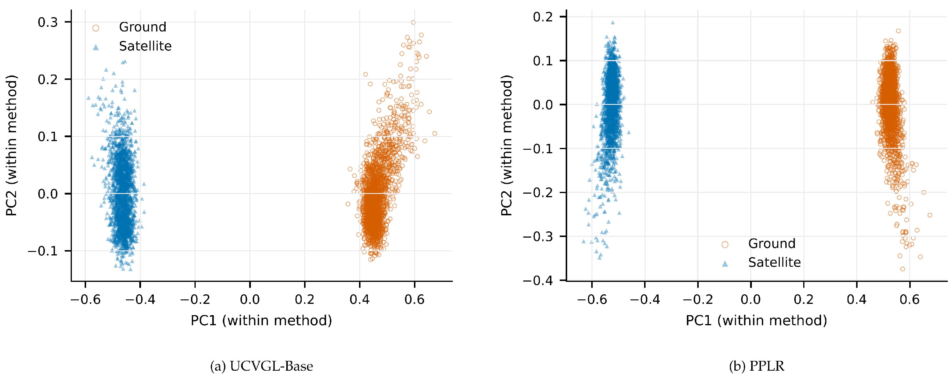
Figure 9 separates the two similarity terms that form the diagnostic ground-truth margin. The PPLR GT-positive density is concentrated at higher similarity values than the UCVGL-Base density, while the hardest-negative distribution also shifts rather than being uniformly suppressed. The two marginal distributions should therefore be read jointly with the query-level margin in Figure 8b: neither marginal alone determines a query’s retrieval rank, and the observed shifts do not establish a causal mechanism. The corresponding feature-space visualization is shown in Figure 10; PCA is fitted separately for each method, so absolute coordinates across panels are not directly comparable.

Taken together, the qualitative and diagnostic plots provide complementary evidence. The examples include improvements, a common failure, and a regression, so they illustrate both the benefit and the limits of pseudo-label refinement. Figure 8 and Figure 9 summarize all 8884 CVUSA Test queries, whereas Figure 10 uses a fixed 2000-query subset and independent method-wise PCA fits. The PCA panels can therefore illustrate within-method view structure, but cannot be used to claim that one method occupies a globally closer or better absolute coordinate system. These plots support descriptive observations about retrieval behavior and separability; they do not establish a causal mechanism or a population-level error decomposition.

For computational context, PPLR adds a pseudo-label selection and refresh workload to the ordinary feature-extraction and similarity-inference path. The measured profiles separate feature extraction, candidate selection, and a bounded 200-step update block; they therefore describe the relative workload of the added operations rather than an end-to-end training duration. The fixed update block is reported as a bounded profile and is not a complete training-time estimate.

5.10. Semi-Supervised GT-Ratio Context

To provide supervision-ratio context without changing the main 0% paired-GT protocol,

Table 11. Semi-supervised CVACT Val GT-ratio context under the separately reported ConvNeXt-Small/$224\times 224$ recipe. UCVGL values are from the published semi-supervised comparison.

Method	GT Ratio	R@1	R@5	R@10
PPLR (Ours)	0.1%	13.98	29.13	37.81
	0.5%	85.81	94.72	96.09
	1%	86.05	94.74	96.11
	5%	86.15	95.24	96.57
	10%	86.21	95.44	96.53
	20%	86.31	95.48	96.83
UCVGL [8]	1%	68.29	85.18	88.80
	5%	78.10	90.87	93.11
	10%	78.88	91.31	93.53
	20%	79.60	91.98	93.96
	100%	84.44	94.85	98.53

summarizes a separate ConvNeXt-Small/$224\times 224$ semi-supervised CVACT recipe. The fixed GT ratios supply paired anchors (35, 177, 355, 1776, 3553, or 7106 pairs); anchors are merged as trusted identity pairs, while other locations use the coverage-entrance curriculum and query gate. The PPLR rows use 40 epochs and seed 42. UCVGL rows are reported from its published semi-supervised table, where labeled correspondences are combined with dynamically refined pseudo-labels under that protocol. This Small/224 comparison is not a matched fully supervised ConvNeXt-Base/$384\times 384$ experiment and is not a direct replacement for the main Base result.

Within the separate Small/224 recipe, performance rises sharply between 0.1% and 0.5% paired GT and then changes more gradually across the tested ratios. These values should not be compared directly with the main 0% PPLR Base result because the encoder, input resolution, training recipe, and supervision protocol differ. The ratio sweep is available for CVACT Val only, and no ratio-resolved CVACT Test claim is made.

6. Discussion

6.1. Interpretation of Main Results

Building on the quantitative comparisons in Section 5.3, we discuss the observed improvement pattern and the scope of the stage-wise design.

The R@1 improvement over UCVGL-Base is +5.26 pp on CVUSA Test, +4.65 pp on CVACT Val, and +6.31 pp on the CVACT Test split. The magnitude differs across splits, but the available evidence does not isolate a dataset-level causal explanation. We therefore interpret the pattern as an empirical result of the evaluated configuration rather than evidence that one geographic property is responsible.

The operation-wise statistics in Table 7 show the evaluated quantity–quality progression within Stage 2: the candidate pool is reduced from reciprocal retrieval to the final retained set while the offline precision diagnostic increases. Because these precision values are computed only after the candidate set is frozen and joined with ground truth, they describe the selected sets and are not training signals. Whether the same pattern holds on other datasets remains open.

6.2. Analysis of Module Complementarity

The three control groups operate as complementary layers within Stage 2. Reciprocal neighborhood retrieval expands the candidate pool beyond strict top-1 matching, allowing candidates whose forward rank is above one to enter the pipeline. The progressive coarse filtering scales the retained set from a small high-reliability seed to broader dataset utilization, providing explicit quantity scheduling. The consistency-guided fine filtering maintains precision through an ensemble of complementary signals—augmentation consistency, margin ranking, and history stability—rather than relying on a single hard threshold.

While the ablation study in Section 5.5 quantifies control-group and fine-grained changes, the grouped and fine-grained rows answer different questions. Removing a grouped coarse or fine control produces larger module-level degradations than removing one operation inside an otherwise active group, which is consistent with complementary controls and partial compensation. These values are not additive contributions and do not establish a complete interaction model or statistical significance.

The candidate-neighborhood sweep in Table 9 varies within a narrow band, with the fixed $k=5$ configuration at the upper end of both tested ranges. Together with the reporting schedule and retention results in Table 8, this indicates robustness to moderate changes in curriculum pace and selectivity rather than a sharply tuned operating point. These parameters are required to specify how candidates are constructed and retained, but the exact values are fixed design choices rather than separate performance claims. The grouped ablations show substantially larger changes when complete control groups are removed; this does not imply that individual changes are additive or establish a causal interaction model.

6.3. Dataset-Specific Dynamics and Transfer Behavior

Dataset-dependent effects are visible in the pseudo-label dynamics. On CVUSA, the recorded precision remains above 0.92 throughout the plotted trajectory, whereas on CVACT, it declines from 0.98 at epoch 4 to 0.87 at epoch 39. These are measured differences in the evaluated runs; the available data do not isolate a scene-level cause. The curves show that expanding the retained set changes the precision profile differently on the two benchmarks. A dataset-adaptive schedule is a possible future direction, but it is not implemented here.

The source-only transfer results (Table 4) are asymmetric across directions and retain a substantial domain gap. They provide evidence of partial transferability under a frozen-checkpoint protocol, not a claim that PPLR resolves cross-dataset shift. Target-domain adaptation and supervised warm-starts use different supervision protocols and are outside the present comparison.

6.4. Stability and Reproducibility

The multi-seed validation provides a stability diagnostic: the reported values vary within the ranges shown in Table 10, and the main result remains the pre-specified checkpoint.

The observed stability is compatible with the use of several signals—retrieval margin, augmentation consistency, and assignment history—within a staged selection process. The available runs do not isolate the effect of each signal or show that one is necessary in every setting; those stronger questions require broader factorial and multi-seed evidence.

6.5. Future Directions

Several directions remain for future work. Schedules and thresholds remain fixed design choices, and an unlabeled automatic selection rule is not implemented. A matched ConvNeXt-Base/$384\times 384$ supervised warm-start experiment is also outside the present 0% paired-ground-truth protocol. Evaluating PPLR under such different supervision settings and under open-world retrieval would test the scope of the current findings.

7. Limitations

The benchmarks use a closed-world, approximately one-to-one protocol and do not test missing matches, distractors, repeated locations, or unequal gallery sizes. The schedules and thresholds are fixed design choices; automatic unlabeled parameter selection is not implemented. The grouped and fine-grained ablations are not a complete factorial or multi-seed study for every row. We do not report a matched ConvNeXt-Base/$384\times 384$ supervised warm-start experiment. The cost measurements cover feature extraction, retrieval, pseudo-label generation, and a fixed 200-step update block rather than an end-to-end training duration. PCA panels use independent fits, so their absolute coordinates should not be compared across methods. Source-only transfer is not target-domain adaptation, and methods with different native tasks or supervision cannot be ranked as direct alternatives. The implementation is not publicly available at this stage; detailed algorithmic descriptions and experimental configurations are provided in the manuscript.

8. Conclusions

We presented PPLR, a two-stage pseudo-label pipeline for fully unsupervised cross-view geo-localization. Under the 0% paired-ground-truth protocol, PPLR reaches R@1 of 96.30 on CVUSA Test, 89.23 on CVACT Val, and 66.84 on the CVACT Test split. Source-only transfer reaches 73.06, 41.35, and 58.79 R@1 in the evaluated directions, improving over the matched UCVGL-Base values while retaining a domain gap. Grouped and fine-grained ablations, sensitivity, mechanism, qualitative, feature, and computational context characterize the evaluated configuration. These analyses do not treat operation effects as additive or claim automatic parameter selection, and the closed-world scope, fixed schedules, protocol differences, and diagnostic nature of the offline GT analyses define the boundaries of the conclusions.

References

1. Workman, S.; Souvenir, R.; Jacobs, N. Wide-Area Image Geolocalization with Aerial Reference Imagery. In Proceedings of the 2015 IEEE International Conference on Computer Vision, ICCV 2015, Santiago, Chile, 7–13 December 2015; IEEE Computer Society: Washington, DC, USA, 2015; pp. 3961–3969. [Google Scholar] [CrossRef] [Scilit]
2. Zhai, M.; Bessinger, Z.; Workman, S.; Jacobs, N. Predicting Ground-Level Scene Layout from Aerial Imagery. In Proceedings of the 2017 IEEE Conference on Computer Vision and Pattern Recognition, CVPR 2017, Honolulu, HI, USA, 21–26 July 2017; IEEE Computer Society: Washington, DC, USA, 2017; pp. 4132–4140. [Google Scholar] [CrossRef] [Scilit]
3. Deuser, F.; Habel, K.; Oswald, N. Sample4Geo: Hard Negative Sampling For Cross-View Geo-Localisation. In Proceedings of the IEEE/CVF International Conference on Computer Vision, ICCV 2023, Paris, France, 1–6 October 2023; IEEE Computer Society: Washington, DC, USA, 2023; pp. 16801–16810. [Google Scholar] [CrossRef] [Scilit]
4. Zhu, S.; Shah, M.; Chen, C. TransGeo: Transformer Is All You Need for Cross-view Image Geo-localization. In Proceedings of the IEEE/CVF Conference on Computer Vision and Pattern Recognition, CVPR 2022, New Orleans, LA, USA, 18–24 June 2022; IEEE Computer Society: Washington, DC, USA, 2022; pp. 1152–1161. [Google Scholar] [CrossRef] [Scilit]
5. Hu, S.; Feng, M.; Nguyen, R.M.H.; Lee, G.H. CVM-Net: Cross-View Matching Network for Image-Based Ground-to-Aerial Geo-Localization. In Proceedings of the 2018 IEEE Conference on Computer Vision and Pattern Recognition, CVPR 2018, Salt Lake City, UT, USA, 18–22 June 2018; Computer Vision Foundation: Scarsdale, NY, USA; IEEE Computer Society: Washington, DC, USA, 2018; pp. 7258–7267. [Google Scholar] [CrossRef] [Scilit]
6. Shi, Y.; Liu, L.; Yu, X.; Li, H. Spatial-Aware Feature Aggregation for Image based Cross-View Geo-Localization. In Proceedings of the Advances in Neural Information Processing Systems 32: Annual Conference on Neural Information Processing Systems 2019, NeurIPS 2019, Vancouver, BC, Canada, 8–14 December 2019; Wallach, H.M., Larochelle, H., Beygelzimer, A., d’Alché-Buc, F., Fox, E.B., Garnett, R., Eds.; Curran Associates, Inc.: Red Hook, NY, USA, 2019; pp. 10090–10100. [Google Scholar]
7. Wang, T.; Zheng, Z.; Yan, C.; Zhang, J.; Sun, Y.; Zheng, B.; Yang, Y. Each Part Matters: Local Patterns Facilitate Cross-View Geo-Localization. IEEE Trans. Circuits Syst. Video Technol. 2022, 32, 867–879. [Google Scholar] [CrossRef] [Scilit]
8. Li, G.; Qian, M.; Xia, G. Unleashing Unlabeled Data: A Paradigm for Cross-View Geo-Localization. In Proceedings of the IEEE/CVF Conference on Computer Vision and Pattern Recognition, CVPR 2024, Seattle, WA, USA, 16–22 June 2024; IEEE Computer Society: Washington, DC, USA, 2024; pp. 16719–16729. [Google Scholar] [CrossRef] [Scilit]
9. Li, H.; Xu, C.; Yang, W.; Yu, H.; Xia, G.S. Learning Cross-View Visual Geo-Localization without Ground Truth. IEEE Trans. Geosci. Remote Sens. 2024, 62, 5632017. [Google Scholar] [CrossRef] [Scilit]
10. Wang, X.; Zhang, L.; Fan, Z.; Liu, Y.; Chen, C.; Deng, F. From Coarse to Fine: A Matching and Alignment Framework for Unsupervised Cross-View Geo-Localization. In Proceedings of the 39th AAAI Conference on Artificial Intelligence, AAAI 2025, Philadelphia, PA, USA, 25 February–4 March 2025; AAAI Press: Washington, DC, USA, 2025; Volume 39, pp. 8024–8032. [Google Scholar] [CrossRef] [Scilit]
11. Lin, T.; Cui, Y.; Belongie, S.J.; Hays, J. Learning deep representations for ground-to-aerial geolocalization. In Proceedings of the IEEE Conference on Computer Vision and Pattern Recognition, CVPR 2015, Boston, MA, USA, 7–12 June 2015; IEEE Computer Society: Washington, DC, USA, 2015; pp. 5007–5015. [Google Scholar] [CrossRef] [Scilit]
12. He, K.; Zhang, X.; Ren, S.; Sun, J. Deep Residual Learning for Image Recognition. In Proceedings of the 2016 IEEE Conference on Computer Vision and Pattern Recognition, CVPR 2016, Las Vegas, NV, USA, 27–30 June 2016; IEEE Computer Society: Washington, DC, USA, 2016; pp. 770–778. [Google Scholar] [CrossRef] [Scilit]
13. Tian, Y.; Chen, C.; Shah, M. Cross-View Image Matching for Geo-Localization in Urban Environments. In Proceedings of the 2017 IEEE Conference on Computer Vision and Pattern Recognition, CVPR 2017, Honolulu, HI, USA, 21–26 July 2017; IEEE Computer Society: Washington, DC, USA, 2017; pp. 3608–3616. [Google Scholar] [CrossRef] [Scilit]
14. Shi, Y.; Yu, X.; Liu, L.; Zhang, T.; Li, H. Optimal Feature Transport for Cross-View Image Geo-Localization. In Proceedings of the The Thirty-Fourth AAAI Conference on Artificial Intelligence, AAAI 2020, The Thirty-Second Innovative Applications of Artificial Intelligence Conference, IAAI 2020, The Tenth AAAI Symposium on Educational Advances in Artificial Intelligence, EAAI 2020, New York, NY, USA, 7–12 February 2020; AAAI Press: Washington, DC, USA, 2020; pp. 11990–11997. [Google Scholar] [CrossRef] [Scilit]
15. Cai, S.; Guo, Y.; Khan, S.H.; Hu, J.; Wen, G. Ground-to-Aerial Image Geo-Localization with a Hard Exemplar Reweighting Triplet Loss. In Proceedings of the 2019 IEEE/CVF International Conference on Computer Vision, ICCV 2019, Seoul, Republic of Korea, 27 October–2 November 2019; IEEE Computer Society: Washington, DC, USA, 2019; pp. 8390–8399. [Google Scholar] [CrossRef] [Scilit]
16. Vaswani, A.; Shazeer, N.; Parmar, N.; Uszkoreit, J.; Jones, L.; Gomez, A.N.; Kaiser, L.; Polosukhin, I. Attention is All you Need. In Proceedings of the Advances in Neural Information Processing Systems 30: Annual Conference on Neural Information Processing Systems 2017, Long Beach, CA, USA, 4–9 December 2017; Guyon, I., von Luxburg, U., Bengio, S., Wallach, H.M., Fergus, R., Vishwanathan, S.V.N., Garnett, R., Eds.; Curran Associates, Inc.: Red Hook, NY, USA, 2017; pp. 5998–6008. [Google Scholar]
17. Dosovitskiy, A.; Beyer, L.; Kolesnikov, A.; Weissenborn, D.; Zhai, X.; Unterthiner, T.; Dehghani, M.; Minderer, M.; Heigold, G.; Gelly, S.; et al. An Image is Worth 16x16 Words: Transformers for Image Recognition at Scale. In Proceedings of the 9th International Conference on Learning Representations, ICLR 2021, Virtual Event, 3–7 May 2021; OpenReview.net: Alameda, CA, USA, 2021. [Google Scholar]
18. Li, C.; Yan, C.; Xiang, X.; Lai, J.; Zhou, H.; Tang, D. HADGEO: Image Based 3-DoF Cross-View Geo-Localization with Hard Sample Mining. In Proceedings of the ICASSP 2024—2024 IEEE International Conference on Acoustics, Speech and Signal Processing (ICASSP); IEEE Computer Society: Washington, DC, USA, 2024; pp. 3520–3524. [Google Scholar] [CrossRef] [Scilit]
19. Li, C.; Yan, C.; Xiang, X.; Lai, J.; Zhou, H.; Tang, D. AMPLE: Automatic Progressive Learning for Orientation Unknown Ground-to-Aerial Geo-Localization. IEEE Trans. Geosci. Remote Sens. 2025, 63, 5800115. [Google Scholar] [CrossRef] [Scilit]
20. Zhang, X.; Li, X.; Sultani, W.; Zhou, Y.; Wshah, S. Cross-View Geo-Localization via Learning Disentangled Geometric Layout Correspondence. In Proceedings of the Thirty-Seventh AAAI Conference on Artificial Intelligence, AAAI 2023, Thirty-Fifth Conference on Innovative Applications of Artificial Intelligence, IAAI 2023, Thirteenth Symposium on Educational Advances in Artificial Intelligence, EAAI 2023, Washington, DC, USA, 7–14 February 2023; Williams, B., Chen, Y., Neville, J., Eds.; AAAI Press: Washington, DC, USA, 2023; pp. 3480–3488. [Google Scholar] [CrossRef] [Scilit]
21. Zhang, X.; Li, X.; Sultani, W.; Chen, C.; Wshah, S. GeoDTR+: Toward Generic Cross-View Geolocalization via Geometric Disentanglement. IEEE Trans. Pattern Anal. Mach. Intell. 2024, 46, 10419–10433. [Google Scholar] [CrossRef] [Scilit] [PubMed]
22. Yang, H.; Lu, X.; Zhu, Y. Cross-view Geo-localization with Layer-to-Layer Transformer. In Proceedings of the Advances in Neural Information Processing Systems 34: Annual Conference on Neural Information Processing Systems 2021, NeurIPS 2021, Virtual, 6–14 December 2021; Ranzato, M., Beygelzimer, A., Dauphin, Y.N., Liang, P., Vaughan, J.W., Eds.; Curran Associates, Inc.: Red Hook, NY, USA, 2021; pp. 29009–29020. [Google Scholar]
23. Ye, J.; Lv, Z.; Li, W.; Yu, J.; Yang, H.; Zhong, H.; He, C. Cross-View Image Geo-Localization with Panorama-BEV Co-retrieval Network. In Proceedings of the Computer Vision—ECCV 2024—18th European Conference, Milan, Italy, 29 September–4 October 2024, Proceedings, Part XXXVII; Leonardis, A., Ricci, E., Roth, S., Russakovsky, O., Sattler, T., Varol, G., Eds.; Lecture Notes in Computer Science; Springer: Cham, Switzerland, 2024; pp. 74–90. [Google Scholar] [CrossRef] [Scilit]
24. Wang, Y.; Zhang, J.; Wei, R.; Gao, W.; Wang, Y. MFRGN: Multi-scale Feature Representation Generalization Network for Ground-to-Aerial Geo-localization. In Proceedings of the 32nd ACM International Conference on Multimedia, MM 2024, Melbourne, VIC, Australia, 28 October–1 November 2024; Cai, J., Kankanhalli, M.S., Prabhakaran, B., Boll, S., Subramanian, R., Zheng, L., Singh, V.K., César, P., Xie, L., Xu, D., Eds.; ACM: New York, NY, USA, 2024; pp. 2574–2583. [Google Scholar] [CrossRef] [Scilit]
25. Zhang, Q.; Zhu, Y. Aligning Geometric Spatial Layout in Cross-View Geo-Localization via Feature Recombination. In Proceedings of the Thirty-Eighth AAAI Conference on Artificial Intelligence, AAAI 2024, Thirty-Sixth Conference on Innovative Applications of Artificial Intelligence, IAAI 2024, Fourteenth Symposium on Educational Advances in Artificial Intelligence, EAAI 2024, Vancouver, BC, Canada, 20–27 February 2024; Wooldridge, M.J., Dy, J.G., Natarajan, S., Eds.; AAAI Press: Washington, DC, USA, 2024; pp. 7251–7259. [Google Scholar] [CrossRef] [Scilit]
26. Zhang, Y.; Zhang, X.; Sun, G.; Lyu, Z.; Wshah, S.; Chen, C. Geo2: Geometry-Guided Cross-view Geo-Localization and Image Synthesis. In Proceedings of the IEEE/CVF Conference on Computer Vision and Pattern Recognition (CVPR), 2026; Computer Vision Foundation: Scarsdale, NY, USA, 2026; pp. 19432–19442. [Google Scholar]
27. Wang, R.; Yuan, W.; Yuan, W.; Liu, T.; Xi, X.; Zhu, Y. GenGeo: Robust Cross-View Geo-Localization via Foundation Model and Dynamic Feature Aggregation. Remote Sens. 2026, 18, 1116. [Google Scholar] [CrossRef] [Scilit]
28. Shen, J.; Chen, L.; Bai, Y.; Miao, Z.; Qu, Z.; Zhou, P.; Li, J. Augmenting Cross-View Geo-Localization with Spatial Semantics from Vision Foundation Models. In Proceedings of the ACM Web Conference 2026, WWW 2026, Dubai, United Arab Emirates, Originally Scheduled for 13–17 April 2026, Rescheduled for 29 June–3 July 2026; Hacid, H., Maarek, Y., Bonchi, F., Guy, I., Yilmaz, E., Eds.; ACM: New York, NY, USA, 2026; pp. 5177–5188. [Google Scholar] [CrossRef] [Scilit]
29. Wu, L.; Lv, B.; Ouyang, S.; Zhu, Y. MRGeo: Robust Cross-View Geo-Localization of Corrupted Images via Spatial and Channel Feature Enhancement. In Proceedings of the Fortieth AAAI Conference on Artificial Intelligence, Thirty-Eighth Conference on Innovative Applications of Artificial Intelligence, Sixteenth Symposium on Educational Advances in Artificial Intelligence, AAAI 2026, Singapore, 20–27 January 2026; Koenig, S., Jenkins, C., Taylor, M.E., Eds.; AAAI Press: Washington, DC, USA, 2026; pp. 10691–10699. [Google Scholar] [CrossRef] [Scilit]
30. Huang, J.; Wu, M.; Li, P.; Wu, W.; Yu, R. VimGeo: Efficient Cross-View Geo-Localization with Vision Mamba Architecture. In Proceedings of the Thirty-Fourth International Joint Conference on Artificial Intelligence, IJCAI 2025, Montreal, QC, Canada, 16–22 August 2025; ijcai.org: Darmstadt, Germany, 2025; pp. 1188–1196. [Google Scholar] [CrossRef] [Scilit] [PubMed]
31. Shi, Y.; Li, H. Beyond Cross-view Image Retrieval: Highly Accurate Vehicle Localization Using Satellite Image. In Proceedings of the IEEE/CVF Conference on Computer Vision and Pattern Recognition, CVPR 2022, New Orleans, LA, USA, 18–24 June 2022; IEEE Computer Society: Washington, DC, USA, 2022; pp. 16989–16999. [Google Scholar] [CrossRef] [Scilit]
32. Shi, Y.; Yu, X.; Campbell, D.; Li, H. Where Am I Looking At? Joint Location and Orientation Estimation by Cross-View Matching. In Proceedings of the 2020 IEEE/CVF Conference on Computer Vision and Pattern Recognition, CVPR 2020, Seattle, WA, USA, 13–19 June 2020; Computer Vision Foundation: Scarsdale, NY, USA; IEEE Computer Society: Washington, DC, USA, 2020; pp. 4064–4072. [Google Scholar] [CrossRef] [Scilit]
33. Lin, J.; Zheng, Z.; Zhong, Z.; Luo, Z.; Li, S.; Yang, Y.; Sebe, N. Joint Representation Learning and Keypoint Detection for Cross-View Geo-Localization. IEEE Trans. Image Process. 2022, 31, 3780–3792. [Google Scholar] [CrossRef] [Scilit] [PubMed]
34. Lee, D.H. Pseudo-Label: The Simple and Efficient Semi-Supervised Learning Method for Deep Neural Networks. In Proceedings of the Workshop on Challenges in Representation Learning, ICML, 2013; JMLR.org: Cambridge, MA, USA, 2013; Volume 3, p. 896. [Google Scholar]
35. Arazo, E.; Ortego, D.; Albert, P.; O’Connor, N.E.; McGuinness, K. Pseudo-Labeling and Confirmation Bias in Deep Semi-Supervised Learning. In Proceedings of the 2020 International Joint Conference on Neural Networks, IJCNN 2020, Glasgow, UK, 19–24 July 2020; IEEE Computer Society: Washington, DC, USA, 2020; pp. 1–8. [Google Scholar] [CrossRef] [Scilit]
36. Bengio, Y.; Louradour, J.; Collobert, R.; Weston, J. Curriculum learning. In Proceedings of the 26th Annual International Conference on Machine Learning, ICML 2009, Montreal, QC, Canada, 14–18 June 2009; Danyluk, A.P., Bottou, L., Littman, M.L., Eds.; ACM International Conference Proceeding Series; ACM: New York, NY, USA, 2009; pp. 41–48. [Google Scholar] [CrossRef] [Scilit]
37. Kong, Y.; Liu, L.; Wang, J.; Tao, D. Adaptive Curriculum Learning. In Proceedings of the 2021 IEEE/CVF International Conference on Computer Vision, ICCV 2021, Montreal, QC, Canada, 10–17 October 2021; IEEE Computer Society: Washington, DC, USA, 2021; pp. 5047–5056. [Google Scholar] [CrossRef] [Scilit]
38. Jiang, L.; Zhou, Z.; Leung, T.; Li, L.; Fei-Fei, L. MentorNet: Learning Data-Driven Curriculum for Very Deep Neural Networks on Corrupted Labels. In Proceedings of the 35th International Conference on Machine Learning, ICML 2018, Stockholmsmässan, Stockholm, Sweden, 10–15 July 2018; Dy, J.G., Krause, A., Eds.; Proceedings of Machine Learning Research; PMLR: Cambridge, MA, USA, 2018; pp. 2304–2313. [Google Scholar]
39. Laine, S.; Aila, T. Temporal Ensembling for Semi-Supervised Learning. In Proceedings of the 5th International Conference on Learning Representations, ICLR 2017, Toulon, France, 24–26 April 2017, Conference Track Proceedings; OpenReview.net: Alameda, CA, USA, 2017. [Google Scholar]
40. Tarvainen, A.; Valpola, H. Mean Teachers Are Better Role Models: Weight-Averaged Consistency Targets Improve Semi-Supervised Deep Learning Results. In Proceedings of the Advances in Neural Information Processing Systems 30: Annual Conference on Neural Information Processing Systems 2017, NeurIPS 2017, Long Beach, CA, USA, 4–9 December 2017; Curran Associates, Inc.: Red Hook, NY, USA, 2017; pp. 1195–1204. [Google Scholar]
41. Sohn, K.; Berthelot, D.; Carlini, N.; Zhang, Z.; Zhang, H.; Raffel, C.; Cubuk, E.D.; Kurakin, A.; Li, C. FixMatch: Simplifying Semi-Supervised Learning with Consistency and Confidence. In Proceedings of the Advances in Neural Information Processing Systems 33: Annual Conference on Neural Information Processing Systems 2020, NeurIPS 2020, Virtual, 6–12 December 2020; Larochelle, H., Ranzato, M., Hadsell, R., Balcan, M., Lin, H., Eds.; Curran Associates, Inc.: Red Hook, NY, USA, 2020; pp. 596–608. [Google Scholar]
42. Zhang, B.; Wang, Y.; Hou, W.; Wu, H.; Wang, J.; Okumura, M.; Shinozaki, T. FlexMatch: Boosting Semi-Supervised Learning with Curriculum Pseudo Labeling. In Proceedings of the Advances in Neural Information Processing Systems 34: Annual Conference on Neural Information Processing Systems 2021, NeurIPS 2021, Virtual, 6–14 December 2021; Ranzato, M., Beygelzimer, A., Dauphin, Y.N., Liang, P., Vaughan, J.W., Eds.; Curran Associates, Inc.: Red Hook, NY, USA, 2021; pp. 18408–18419. [Google Scholar]
43. Wang, Y.; Chen, H.; Heng, Q.; Hou, W.; Fan, Y.; Wu, Z.; Wang, J.; Savvides, M.; Shinozaki, T.; Raj, B.; et al. FreeMatch: Self-adaptive Thresholding for Semi-supervised Learning. In Proceedings of the The Eleventh International Conference on Learning Representations, ICLR 2023, Kigali, Rwanda, 1–5 May 2023; OpenReview.net: Alameda, CA, USA, 2023. [Google Scholar]
44. Xu, Y.; Shang, L.; Ye, J.; Qian, Q.; Li, Y.; Sun, B.; Li, H.; Jin, R. Dash: Semi-Supervised Learning with Dynamic Thresholding. In Proceedings of the 38th International Conference on Machine Learning, ICML 2021, Virtual Event, 18–24 July 2021; Meila, M., Zhang, T., Eds.; Proceedings of Machine Learning Research; PMLR: Cambridge, MA, USA, 2021; pp. 11525–11536. [Google Scholar]
45. Guo, L.; Li, Y. Class-Imbalanced Semi-Supervised Learning with Adaptive Thresholding. In Proceedings of the International Conference on Machine Learning, ICML 2022, Baltimore, MD, USA, 17–23 July 2022; Chaudhuri, K., Jegelka, S., Song, L., Szepesvári, C., Niu, G., Sabato, S., Eds.; Proceedings of Machine Learning Research; PMLR: Cambridge, MA, USA, 2022; pp. 8082–8094. [Google Scholar]
46. Berthelot, D.; Carlini, N.; Goodfellow, I.J.; Papernot, N.; Oliver, A.; Raffel, C. MixMatch: A Holistic Approach to Semi-Supervised Learning. In Proceedings of the Advances in Neural Information Processing Systems 32: Annual Conference on Neural Information Processing Systems 2019, NeurIPS 2019, Vancouver, BC, Canada, 8–14 December 2019; Wallach, H.M., Larochelle, H., Beygelzimer, A., d’Alché-Buc, F., Fox, E.B., Garnett, R., Eds.; Curran Associates, Inc.: Red Hook, NY, USA, 2019; pp. 5050–5060. [Google Scholar]
47. Xie, Q.; Dai, Z.; Hovy, E.H.; Luong, T.; Le, Q. Unsupervised Data Augmentation for Consistency Training. In Proceedings of the Advances in Neural Information Processing Systems 33: Annual Conference on Neural Information Processing Systems 2020, NeurIPS 2020, Virtual, 6–12 December 2020; Larochelle, H., Ranzato, M., Hadsell, R., Balcan, M., Lin, H., Eds.; Curran Associates, Inc.: Red Hook, NY, USA, 2020; pp. 6256–6268. [Google Scholar]
48. Wei, C.; Sohn, K.; Mellina, C.; Yuille, A.L.; Yang, F. CReST: A Class-Rebalancing Self-Training Framework for Imbalanced Semi-Supervised Learning. In Proceedings of the IEEE Conference on Computer Vision and Pattern Recognition, CVPR 2021, Virtual, 19–25 June 2021; Computer Vision Foundation: Scarsdale, NY, USA; IEEE Computer Society: Washington, DC, USA, 2021; pp. 10857–10866. [Google Scholar] [CrossRef] [Scilit]
49. Chen, C.; Chen, Q.; Yang, B.; Zhang, X. UniABG: Unified Adversarial View Bridging and Graph Correspondence for Unsupervised Cross-View Geo-Localization. In Proceedings of the Fortieth AAAI Conference on Artificial Intelligence; AAAI Press: Washington, DC, USA, 2026; Volume 40, pp. 2823–2831. [Google Scholar] [CrossRef] [Scilit]
50. Yuan, Y.; Guo, J.; Zhu, R.; Li, N.; Li, Z.; Luo, W. Towards Pseudo-Labeling with Dynamic Thresholds for Cross-View Image Geolocalization. Remote Sens. 2026, 18, 944. [Google Scholar] [CrossRef] [Scilit]
51. Toker, A.; Zhou, Q.; Maximov, M.; Leal-Taixé, L. Coming Down to Earth: Satellite-to-Street View Synthesis for Geo-Localization. In Proceedings of the IEEE Conference on Computer Vision and Pattern Recognition, CVPR 2021, Virtual, 19–25 June 2021; Computer Vision Foundation: Scarsdale, NY, USA; IEEE Computer Society: Washington, DC, USA, 2021; pp. 6488–6497. [Google Scholar] [CrossRef] [Scilit]
52. Regmi, K.; Shah, M. Bridging the Domain Gap for Ground-to-Aerial Image Matching. In Proceedings of the 2019 IEEE/CVF International Conference on Computer Vision, ICCV 2019, Seoul, Republic of Korea, 27 October–2 November 2019; IEEE Computer Society: Washington, DC, USA, 2019; pp. 470–479. [Google Scholar] [CrossRef] [Scilit]
53. Xia, Z.; Booij, O.; Manfredi, M.; Kooij, J.F.P. Geographically Local Representation Learning with a Spatial Prior for Visual Localization. In Proceedings of the Computer Vision—ECCV 2020 Workshops—Glasgow, UK, 23–28 August 2020, Proceedings, Part II; Bartoli, A., Fusiello, A., Eds.; Lecture Notes in Computer Science; Springer: Cham, Switzerland, 2020; pp. 557–573. [Google Scholar] [CrossRef] [Scilit]
54. Mi, L.; Xu, C.; Castillo-Navarro, J.; Montariol, S.; Yang, W.; Bosselut, A.; Tuia, D. ConGeo: Robust Cross-View Geo-Localization Across Ground View Variations. In Proceedings of the Computer Vision—ECCV 2024—18th European Conference, Milan, Italy, 29 September–4 October 2024, Proceedings, Part XIV; Leonardis, A., Ricci, E., Roth, S., Russakovsky, O., Sattler, T., Varol, G., Eds.; Lecture Notes in Computer Science; Springer: Cham, Switzerland, 2024; pp. 214–230. [Google Scholar] [CrossRef] [Scilit]
55. He, K.; Fan, H.; Wu, Y.; Xie, S.; Girshick, R.B. Momentum Contrast for Unsupervised Visual Representation Learning. In Proceedings of the 2020 IEEE/CVF Conference on Computer Vision and Pattern Recognition, CVPR 2020, Seattle, WA, USA, 13–19 June 2020; Computer Vision Foundation: Scarsdale, NY, USA; IEEE Computer Society: Washington, DC, USA, 2020; pp. 9726–9735. [Google Scholar] [CrossRef] [Scilit]
56. Chen, T.; Kornblith, S.; Norouzi, M.; Hinton, G.E. A Simple Framework for Contrastive Learning of Visual Representations. In Proceedings of the 37th International Conference on Machine Learning, ICML 2020, Virtual Event, 13–18 July 2020; Proceedings of Machine Learning Research; PMLR: Cambridge, MA, USA, 2020; pp. 1597–1607. [Google Scholar]
57. Tian, Y.; Sun, C.; Poole, B.; Krishnan, D.; Schmid, C.; Isola, P. What Makes for Good Views for Contrastive Learning? In Proceedings of the Advances in Neural Information Processing Systems 33: Annual Conference on Neural Information Processing Systems 2020, NeurIPS 2020, Virtual, 6–12 December 2020; Larochelle, H., Ranzato, M., Hadsell, R., Balcan, M., Lin, H., Eds.; Curran Associates, Inc.: Red Hook, NY, USA, 2020; pp. 6827–6839. [Google Scholar]
58. Caron, M.; Misra, I.; Mairal, J.; Goyal, P.; Bojanowski, P.; Joulin, A. Unsupervised Learning of Visual Features by Contrasting Cluster Assignments. In Proceedings of the Advances in Neural Information Processing Systems 33: Annual Conference on Neural Information Processing Systems 2020, NeurIPS 2020, Virtual, 6–12 December 2020; Larochelle, H., Ranzato, M., Hadsell, R., Balcan, M., Lin, H., Eds.; Curran Associates, Inc.: Red Hook, NY, USA, 2020; pp. 9912–9924. [Google Scholar]
59. Grill, J.; Strub, F.; Altché, F.; Tallec, C.; Richemond, P.H.; Buchatskaya, E.; Doersch, C.; Pires, B.Á.; Guo, Z.; Azar, M.G.; et al. Bootstrap Your Own Latent - A New Approach to Self-Supervised Learning. In Proceedings of the Advances in Neural Information Processing Systems 33: Annual Conference on Neural Information Processing Systems 2020, NeurIPS 2020, Virtual, 6–12 December 2020; Larochelle, H., Ranzato, M., Hadsell, R., Balcan, M., Lin, H., Eds.; Curran Associates, Inc.: Red Hook, NY, USA, 2020; pp. 21271–21284. [Google Scholar]
60. Chen, X.; He, K. Exploring Simple Siamese Representation Learning. In Proceedings of the IEEE Conference on Computer Vision and Pattern Recognition, CVPR 2021, Virtual, 19–25 June 2021; Computer Vision Foundation: Scarsdale, NY, USA; IEEE Computer Society: Washington, DC, USA, 2021; pp. 15750–15758. [Google Scholar] [CrossRef] [Scilit]
61. Zhu, S.; Yang, T.; Chen, C. VIGOR: Cross-View Image Geo-Localization Beyond One-to-One Retrieval. In Proceedings of the IEEE Conference on Computer Vision and Pattern Recognition, CVPR 2021, Virtual, 19–25 June 2021; Computer Vision Foundation: Scarsdale, NY, USA; IEEE Computer Society: Washington, DC, USA, 2021; pp. 3640–3649. [Google Scholar] [CrossRef] [Scilit]
62. Zheng, Z.; Wei, Y.; Yang, Y. University-1652: A Multi-view Multi-source Benchmark for Drone-based Geo-localization. In Proceedings of the MM ’20: The 28th ACM International Conference on Multimedia, Virtual Event/Seattle, WA, USA, 12–16 October 2020; Chen, C.W., Cucchiara, R., Hua, X., Qi, G., Ricci, E., Zhang, Z., Zimmermann, R., Eds.; ACM: New York, NY, USA, 2020; pp. 1395–1403. [Google Scholar] [CrossRef] [Scilit]
63. Liu, L.; Li, H. Lending Orientation to Neural Networks for Cross-View Geo-Localization. In Proceedings of the IEEE Conference on Computer Vision and Pattern Recognition, CVPR 2019, Long Beach, CA, USA, 16–20 June 2019; Computer Vision Foundation: Scarsdale, NY, USA; IEEE Computer Society, 2019; pp. 5624–5633. [Google Scholar] [CrossRef] [Scilit]
64. Liu, Z.; Mao, H.; Wu, C.; Feichtenhofer, C.; Darrell, T.; Xie, S. A ConvNet for the 2020s. In Proceedings of the IEEE/CVF Conference on Computer Vision and Pattern Recognition, CVPR 2022, New Orleans, LA, USA, 18–24 June 2022; IEEE Computer Society: Washington, DC, USA, 2022; pp. 11966–11976. [Google Scholar] [CrossRef] [Scilit]
65. Loshchilov, I.; Hutter, F. SGDR: Stochastic Gradient Descent with Warm Restarts. In Proceedings of the 5th International Conference on Learning Representations, ICLR 2017, Toulon, France, 24–26 April 2017, Conference Track Proceedings; OpenReview.net: Alameda, CA, USA, 2017. [Google Scholar]
Figure 1. Overview of the two-stage PPLR training pipeline. Stage 1 (cold-start initialization) converts ground images into fake satellite views and performs intra-view learning, ground–fake cross-view learning, and lightweight pair-quality weighting to obtain the cold-start checkpoint. Stage 2 (progressive pseudo-label learning) extracts features from real ground and satellite images, applies the control operations detailed in Figure 2, and iteratively updates the model to the final checkpoint. Paired ground truth is not used during training; it is used only for evaluation and offline diagnostics.
Remotesensing 18 02714 g001
Figure 2. Control operations within Stage 2. At iteration i, the current checkpoint extracts ground and satellite features to construct a cross-view similarity matrix. Candidate ground–satellite pairs are first expanded by reciprocal neighborhood retrieval, then filtered by margin-based coarse filtering with a margin threshold and progressive keep-ratio, and finally refined by consistency-guided fine filtering with consistency pre-filtering, retrieval-margin ranking, history tie-breaking, and a fine-filter retention ratio. The retained pseudo-labels are used for InfoNCE training to produce the next checkpoint; these operations are controls within Stage 2, not additional training stages.
Remotesensing 18 02714 g002
Figure 3. Epoch-wise pseudo-label dynamics retained from the original analysis. Candidate and pseudo-label coverage are shown on the left axis and precision on the right; these curves provide trajectory context, while the revised canonical operation-wise statistics are reported in Figure 4 and Table 7.
Remotesensing 18 02714 g003
Figure 4. Operation-wise selection statistics within Stage 2 on the CVACT training selection. (a) Reciprocal candidates binned by forward rank: Rank 1, 2–5, 6–10, and >10. (b) Nested candidate counts (bars, left axis) and coverage relative to 35,532 CVACT training locations (green circles, right axis) after raw retrieval, threshold gating, coarse truncation, consistency checking, and fine retention. (c) Offline precision (red triangles) and adjacent retention (blue squares) for the same snapshots. Ground truth is joined only after each candidate set is frozen; precision is therefore a diagnostic rather than a training signal.
Remotesensing 18 02714 g004
Figure 5. Top-k sensitivity: R@1 convergence curves during pseudo-label learning. Insets show epochs 33–36 and provide convergence context for the endpoint comparisons.
Remotesensing 18 02714 g005
Figure 6. Mean R@1 convergence on CVACT Val across five seeds. Thin lines show the individual trajectories for seeds 39–43, the thick line shows their mean, and shading gives the descriptive 95% confidence interval.
Remotesensing 18 02714 g006
Figure 7. CVUSA qualitative retrieval cases. The examples include improvements, a common failure, and a regression. The panel is illustrative and does not replace aggregate evaluation.
Remotesensing 18 02714 g007
Figure 8. CVUSA retrieval behavior diagnostics on the same 8884 CVUSA Test queries. (a) The empirical CDF of the ground-truth rank uses a logarithmic rank axis; a higher curve at a given rank means more queries have their ground truth within that rank. (b) The empirical CDF of the diagnostic ground-truth margin, defined as ground-truth similarity minus hardest-negative similarity; the black vertical line marks zero margin, and colored dashed lines mark the UCVGL-Base and PPLR medians. (c) A log–log hexbin of paired ground-truth ranks; hexbin colors encode the log-scaled number of queries per bin, and the red dashed line is the equal-rank diagonal; points below it indicate a numerically smaller PPLR rank, and points above it indicate a regression. The displayed Spearman value is the descriptive association between UCVGL and PPLR ground-truth-positive similarities for the same query/ground-truth pairs, not a rank correlation or causal effect.
Remotesensing 18 02714 g008
Figure 9. CVUSA similarity distributions over all 8884 Test queries. (a) Ground-truth-positive similarity and (b) hardest-negative similarity, where the hardest negative is the highest-scoring non-ground-truth gallery item. The curves describe the UCVGL-Base and PPLR marginal distributions; they do not by themselves encode query-wise pairing or causality.
Remotesensing 18 02714 g009
Figure 10. CVUSA feature-space visualization on a fixed subset of 2000 query locations. (a) UCVGL-Base and (b) PPLR each show ground-query points (open circles) and their matched satellite points (triangles) in a joint two-dimensional PCA projection fitted for that method. The panels should be read within method, to inspect the relative arrangement and spread of the two views. PCA is fitted separately for each method; absolute coordinates, rotations, and inter-panel distances are therefore not directly comparable. The visualization is diagnostic rather than a causal explanation of the retrieval gains.
Remotesensing 18 02714 g010