Article

Wind Direction Retrieval from X-Band Marine Radar Images Using 2D-DTCWT–CSC and Maximum-Energy Radial Rings

1
College of Intelligent Systems Science and Engineering, Harbin Engineering University, Harbin 150001, China
2
School of Low-Altitude Equipment and Intelligent Control, Guangzhou Maritime University, Guangzhou 510725, China
3
College of Electrical Engineering and Automation, Luoyang Normal University, No. 6 Jiqing Road, Luoyang 471934, China
*
Author to whom correspondence should be addressed.
Remote Sens. 2026, 18(16), 2728; https://doi.org/10.3390/rs18162728
Submission received: 6 July 2026 / Revised: 11 August 2026 / Accepted: 12 August 2026 / Published: 13 August 2026
(This article belongs to the Special Issue Feature Paper Special Issue on Ocean Remote Sensing (Third Edition))

Abstract

Under moderate-to-high wind conditions, low-frequency wind direction modulation signals in X-band marine radar images are strongly coupled with wave textures, sea clutter, and blind-zone interference, which degrades wind direction retrieval accuracy. To address this problem, this study proposes a wind direction retrieval method based on two-dimensional dual-tree complex wavelet transform (2D-DTCWT), convolutional sparse coding (CSC), and maximum-energy radial rings. First, 2D-DTCWT is used to suppress wave textures and local noise in the wavelet domain while enhancing low-frequency wind direction modulation signals. Then, K–singular value decomposition (K-SVD) learns the energy distribution characteristics of wind signals, and CSC obtains the spatial response distribution of wind energy in radar images. Finally, the maximum-energy radial ring is adaptively identified, and azimuthal energy statistics within this ring are fitted using a cosine-squared function. The proposed method was evaluated using X-band marine radar data collected during sea trials in the coastal waters of Zhejiang, China. On the 900-sample main validation dataset, the proposed method achieved the highest correlation coefficient (CC) of 0.85 and an overall root mean square error (RMSE) of 4.24°, reducing the RMSE by 43.0% and 66.7% compared with conventional single-curve fitting and extended-bow-heading DWT, respectively. The results demonstrate improved robustness under both upwind and downwind blind-zone conditions.

1. Introduction

Surface wind fields are a primary driver of ocean wave generation and evolution [1]. Marine wind and wave data are essential for naval vessel operations, navigation safety, route planning, and offshore engineering [2]. The strength and stability of the sea surface wind field also affect the safe takeoff and landing of shipborne aircraft [3]. Therefore, real-time monitoring of sea surface wind fields is important for maritime safety. As a key wind field parameter, wind direction must be accurately retrieved to support practical engineering applications [4].
At present, sea surface wind direction is measured mainly by two approaches. The first is direct in situ measurement [5,6], which uses instruments such as wind vanes and anemometers [7] installed at land-based stations, buoys, and ships to obtain real-time wind direction data [8,9]. However, in situ measurements are limited by severe weather, difficult offshore operations, and the high cost of deploying sensors over large ocean areas. With advances in remote sensing, satellite- and aircraft-borne microwave scatterometers and synthetic aperture radar (SAR) [10], together with shore-based high-frequency (HF) radar [11,12,13], have been widely used for marine wind-field observation and retrieval. These methods are effective for large-scale measurements but cannot provide continuous real-time wind direction data within a 1 km radius of a vessel because of their broad coverage and limited temporal continuity. Therefore, marine radar-based wind direction retrieval has attracted increasing attention. By exploiting sea clutter images and the backscattering mechanism of marine radar, wave-related characteristics can be extracted from radar cross section information [14]. Thus, the second approach retrieves wind direction from sea clutter images generated by marine radar backscatter. In addition to wind direction, wind speed is also a critical parameter for sea surface wind-field retrieval using marine radar. Previous studies have shown that echo intensity, texture features, and energy distributions in X-band marine radar images are closely related to sea surface wind speed; therefore, wind speed can be estimated using empirical models or data-driven approaches. For example, third-order polynomial models [15] have been used to retrieve sea surface wind speed by establishing empirical relationships between radar echo characteristics and wind speed. More recently, deep learning approaches, such as WSTCNN [16], have further improved wind speed estimation by exploiting multiscale texture features extracted from radar images. These studies indicate that marine radar images contain information associated with both wind speed and wind direction; however, this study focuses specifically on wind direction retrieval under complex sea conditions and radar blind-zone interference.
Algorithms for retrieving sea surface wind direction from marine radar images can be broadly classified into two categories. The first category relies on imaging features modulated by the sea surface wind field. Dankert et al. [17,18,19] conducted detailed investigations of wind-streak features in X-band marine radar images. These features appear as low-frequency patterns at spatial scales of 200–500 m, with orientations approximately parallel to the wind direction. Based on this observation, they proposed the local gradient method (LGM), which analyzes radar image sequences containing wind streaks and identifies the dominant gradient direction perpendicular to the streak orientation to retrieve wind direction. Their results demonstrated that wind streaks in marine radar images can be effectively used for sea surface wind direction retrieval. By investigating the wind-modulated imaging process, Wang et al. [20] determined that the lower spatial-scale limit of small-scale wind streaks is 200 m. Wang further proposed an adaptive reduction method (ARM) for sea surface wind-direction retrieval, in which a reduction factor is introduced to achieve an optimal balance between image resolution and wind-streak preservation. Compared with the conventional local gradient method (LGM), ARM produces more stable wind-direction retrieval results. Subsequently, Wang et al. [21] proposed the wavelet energy spectrum method (ESM), which applies a scale-separation filter to isolate small-scale wind streaks and then uses a two-dimensional fast Fourier transform (2D FFT) to compute their wavelet energy spectrum. The dominant orientation of the small-scale wind streaks is subsequently determined in the wavelet domain. In recent years, Wang et al. [22] extracted sea surface wind-streak texture features by averaging and preprocessing sequences of X-band marine radar images. The dominant texture direction was then estimated in polar coordinates using the fast-converging gray-level co-occurrence matrix (FC-GLCM), thereby enabling sea surface wind direction retrieval. However, this type of method requires the integration of 32 consecutive images to extract stable streak features, which limits its responsiveness to rapidly changing transient wind fields.
The second approach retrieves sea surface wind direction based on the relationship between radar echo intensity and azimuth. Hatten et al. [23] found that the normalized radar cross section (NRCS) is linearly related to sea surface wind speed, with the peak echo intensity occurring in the downwind direction. However, this method requires unobstructed 360° radar imagery. Lund et al. [24] proposed a single-curve fitting algorithm for radar images with blind spots, in which the least-squares method is used to model the relationship between echo intensity and the cosine of the antenna azimuth angle. However, this approach is susceptible to errors induced by ship motion when the antenna is directed toward the bow. Liu et al. [25] proposed a hyperbolic fitting algorithm that determines the final wind direction by applying a second-order fit to the initial wind-direction estimation results. However, the second-order fitting process is strongly affected by radar shadowing and is therefore constrained by the stability of the marine wind field. Chen et al. [26] proposed a marine radar-based probability density function (PDF) method that can suppress interference from fixed objects on the sea surface but imposes specific requirements on both data quality and equipment configuration. In subsequent studies, Chen et al. [27,28] retrieved wind direction by establishing relationships between wind fields and radar images using various deep learning models. However, the retrieval accuracy varies across models, which limits the general applicability of these methods. Wang and Huang [29], Huang et al. [30], and Liu et al. [31] conducted extensive research on sea surface wind direction retrieval under rainy conditions. Although their method is applicable to wind-direction estimation in rain-contaminated radar images, it still requires unobstructed 360° radar imagery. Yu et al. [32] proposed a two-dimensional discrete wavelet transform (2D-DWT) method incorporating extended bow-heading information, which improves the stability of bow-heading fitting. However, the retrieval results still exhibit substantial errors under complex sea surface conditions. Therefore, to address the susceptibility of low-frequency wind-direction modulation signals in shipborne X-band marine navigation radar images to strong wave textures, nonuniform sea clutter, and radar blind spots under moderate-to-high wind-speed conditions, this study proposes a maximum-energy radial-ring-based sea surface wind direction retrieval method that integrates the two-dimensional dual-tree complex wavelet transform (2D-DTCWT) with convolutional sparse coding (CSC). Unlike conventional methods that rely solely on single-stage filtering or statistics from fixed radial regions, this study constructs a two-stage wind-signal extraction framework that integrates wavelet-domain separation with spatial energy localization through 2D-DTCWT and CSC. In the first stage, the directional selectivity of 2D-DTCWT in the wavelet domain is exploited to suppress interference from wave textures. In the second stage, learning-based CSC is employed to extract the spatial distribution of wind energy. This framework reduces the influence of invalid radial regions, blind-spot distortion, and strong localized noise that may persist after low-frequency filtering, thereby improving the robustness of wind-direction fitting.
The remainder of this paper is organized as follows. Section 2 presents the theoretical methodology. Section 3 describes the proposed algorithmic procedure in detail. Section 4 introduces the experimental data sources and analyzes the corresponding results. Section 5 concludes the paper and discusses future research directions.

2. Methodology

2.1. Azimuthal Dependence of Marine Radar Echo Intensity

The theoretical basis for retrieving sea surface wind fields using marine radar lies in the physical relationship between radar echo intensity and wind-induced sea surface roughness. Surface wind fields act on the sea surface through wind stress, generating directional wind waves, capillary waves, and short gravity waves while modifying the distribution of sea surface roughness. As wind speed increases, sea surface roughness increases, and the radar backscattering response is correspondingly enhanced, which is reflected by an overall increase in the normalized radar cross-section (NRCS) and radar image echo intensity.
From the perspective of radar observation geometry, a marine radar antenna scans periodically in azimuth, with different azimuth angles corresponding to different radar look directions. When the angle between the radar look direction and the sea surface wind direction changes, the illuminated wave facets and their local roughness also vary, causing the echo intensity to exhibit distinct azimuthal modulation. Typically, in the upwind direction, the radar primarily illuminates steeper windward wave slopes with higher local roughness, resulting in the strongest backscatter. In the downwind direction, the echo intensity is generally lower, whereas in the crosswind direction, the effective roughness is the lowest, leading to the weakest echo intensity. Therefore, radar echo intensity typically exhibits a cosine-like or cosine-squared dependence on the antenna azimuth angle.
This azimuthal modulation relationship is jointly influenced by the radar polarization and grazing angle. Under vertical polarization, the echo intensity typically exhibits a bimodal structure with peaks in the upwind and downwind directions, with the upwind peak exceeding the downwind peak. Under horizontal polarization, a bimodal structure may also appear at large grazing angles, whereas at low grazing angles, a single peak typically appears only in the upwind direction. The grazing angle is primarily determined by the radar antenna height and observation distance; variations in this angle affect the radar’s sensitivity to surface roughness differences between windward and leeward wave slopes.
Therefore, based on the physical relationship between marine radar echo intensity and antenna azimuth, sea surface wind direction can be retrieved by analyzing the azimuthal distribution of echo intensity. After range correction, removal of occluded areas, and azimuthal averaging, the relationship between the mean echo intensity σ θ and azimuth angle θ is fitted using least squares with a cosine squared model [24]:
σ θ = a 0 + a 1 cos 2 1 2 θ a 2
where a 0 , a 1 , and a 2 are regression parameters. The wind direction is estimated as a 2 , where the fitted function reaches its maximum. This method essentially exploits the modulation of sea surface roughness and directional wave spectra by the wind field, as well as the ability of azimuthal radar scanning to record these modulation features, thereby enabling remote sensing retrieval of sea surface wind direction. However, when the sea surface wind field is unstable or radar obstructions are present, substantial retrieval errors may occur. Therefore, developing an appropriate method for accurately extracting wind-direction-related signals from marine radar images remains a critical challenge.

2.2. DTCWT

2D-DTCWT has been widely used in image fusion [33,34], denoising [35], feature extraction and processing [36,37], and signal processing [38]. Compared with the conventional discrete wavelet transform (DWT), DTCWT uses two parallel real wavelet trees, denoted as Tree A and Tree B, to construct approximate Hilbert-pair wavelets and achieve complex wavelet decomposition. Thus, its coefficients contain both amplitude and phase information, which improves the characterization of local directionality and approximate shift invariance while reducing artifacts and phase distortions associated with conventional DWT [39].

2.2.1. One-Dimensional Dual-Tree Complex Wavelet Transform (1D-DTCWT)

The DTCWT consists of two one-dimensional filter-bank trees, denoted as Tree A and Tree B [40]:
T A : H ( A ) = { h 0 ( A ) , h 1 ( A ) } , G ( A ) = { g 0 ( A ) , g 1 ( A ) } , T B : H ( B ) = { h 0 ( B ) , h 1 ( B ) } , G ( B ) = { g 0 ( B ) , g 1 ( B ) } .
where H ( · ) and G ( · ) denote the decomposition and reconstruction filter sets, respectively. Within these sets, h i ( · ) and g i ( · ) denote the individual decomposition and reconstruction filters, respectively, with i 0 , 1 . The superscripts ( A ) and ( B ) indicate Tree A and Tree B, and the subscripts 0 and 1 denote low-pass and high-pass filters.
The wavelet functions generated by the two trees satisfy the approximate Hilbert-pair condition:
ψ ( B ) ( t ) H ψ ( A ) ( t ) ,
where H { · } denotes the Hilbert transform operator. The two real-valued bases are then combined to form complex wavelet and scaling functions:
ψ ( t ) = ψ ( A ) ( t ) + j ψ ( B ) ( t ) , ϕ ( t ) = ϕ ( A ) ( t ) + j ϕ ( B ) ( t ) ,
where j = 1 , and ψ ( t ) and ϕ ( t ) denote the complex wavelet and scaling functions, respectively.

2.2.2. Two-Dimensional Dual-Tree Complex Wavelet Transform (2D-DTCWT)

The 2D-DTCWT applies the dual-tree filter-bank structure along the row and column directions. For an input signal f ( x , y ) , the subband coefficients generated by Tree A and Tree B at each decomposition level are
W a b ( A ) ( x , y ) =   f ( x , y ) h a ( A ) [ h b ( A ) ] T , W a b ( B ) ( x , y ) =   f ( x , y ) h a ( B ) [ h b ( B ) ] T , a , b { 0 , 1 } ,
where ∗ denotes two-dimensional convolution, and a and b represent row- and column-direction filtering, respectively. Each tree produces four subbands:
{ L L , L H , H L , H H } = { ( 0 , 0 ) , ( 0 , 1 ) , ( 1 , 0 ) , ( 1 , 1 ) } .
Here, L L is the low-frequency approximation component, while L H , H L , and H H are high-frequency detail components.
Under the approximate Hilbert-pair condition, the complex detail coefficients are obtained by combining the corresponding subbands from the two trees:
W s c ( x , y ) = W s ( A ) ( x , y ) + j W s ( B ) ( x , y ) , s { L H , H L , H H } ,
Here, W s ( q ) is obtained from Equation (5) according to the index mapping in Equation (6), where q A , B . Specifically, W L H ( q ) = W 01 ( q ) , W H L ( q ) = W 10 ( q ) , and W H H ( q ) = W 11 ( q ) .
The output of the 2D-DTCWT at the -th decomposition level is
Y h ( l ) = W θ ( l ) θ ± 15 ° , ± 45 ° , ± 75 ° , Y l ( l ) = W L L ( A , l ) + j W L L ( B , l ) .
Here, W θ ( l ) denotes one of the six directional complex coefficient maps obtained from the LH, HL, and HH high-frequency outputs through the fixed sum-and-difference directional combinations of the parallel filter-bank trees. Each high-frequency subband group produces a pair of oppositely oriented responses, yielding the six directions 75 ° , 45 ° , 15 ° , 15 ° , 45 ° , and 75 ° , where Y h ( l ) represents the six directional complex high-frequency subbands, and Y l ( l ) is the complex low-frequency approximation component used as the input for the next level.
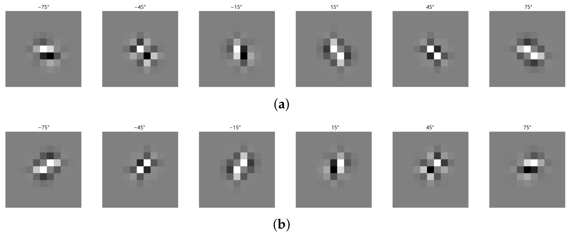
As shown in Figure 1, a single-level 2D-DTCWT generates six approximately oriented high-frequency subbands corresponding to 75 ° , 45 ° , 15 ° , 15 ° , 45 ° , and 75 ° . These subbands provide selective responses to edges and textures with different orientations.
The alternating black and white regions in Figure 1 represent the positive and negative lobes of the band-pass wavelet kernels, while the near-zero background indicates spatial localization. Figure 1a,b show the real and imaginary parts of the complex wavelet basis functions, which approximately form Hilbert pairs with a phase difference close to 90 ° . This quadrature relationship provides stable amplitude and phase representations, improving robustness to local shifts and reducing directional aliasing in conventional real-valued DWT.

2.2.3. Hierarchical Recursive Processing

Let Y l ( l ) ( x , y ) denote the low-frequency approximation component at the -th level, with Y l ( 0 ) ( x , y ) = f ( x , y ) . The next-level 2D-DTCWT decomposition is recursively applied to Y l ( l ) ( x , y ) :
Y h ( l + 1 ) = DTCWT h ( l + 1 ) Y l ( l ) = W 1 ( l + 1 ) , W 2 ( l + 1 ) , , W 6 ( l + 1 ) , Y l ( l + 1 ) = Y l ( l ) Φ l + 1 ( A ) + j Y l ( l ) Φ l + 1 ( B ) ,
The coefficients W 1 ( l + 1 ) , , W 6 ( l + 1 ) are obtained by applying the filtering and directional-combination operations described in Equations (5)–(8) to the low-frequency approximation Y l ( l ) from the preceding level. According to the directional order in Equation (8), W 1 ( l + 1 ) , , W 6 ( l + 1 ) correspond to the directional coefficient maps at 75 ° , 45 ° , 15 ° , 15 ° , 45 ° , and 75 ° , respectively. Only the low-frequency approximation is recursively decomposed, whereas the six directional high-frequency coefficient maps generated at each level are retained, where Φ l + 1 ( A ) and Φ l + 1 ( B ) are the low-pass scaling functions of Tree A and Tree B at the ( l + 1 ) -th level.
After J decomposition levels, the multiscale 2D-DTCWT representation of f ( x , y ) is
DTCWT J ( f ) = Y h ( 1 ) , Y h ( 2 ) , , Y h ( J ) , Y l ( J ) .
The high-frequency coefficient set at the -th level is
Y h ( l ) = W 1 ( l ) , W 2 ( l ) , , W 6 ( l ) , l = 1 , 2 , , J .
where Y h ( l ) contains six directional complex subbands, and Y l ( J ) is the final low-frequency approximation component.

2.2.4. Two-Dimensional Inverse Dual-Tree Complex Wavelet Transform (2D-IDTCWT)

The 2D-IDTCWT reconstructs the image from multilevel complex high-frequency coefficients and the final low-frequency approximation component through upsampling and synthesis filtering. Omitting spatial coordinates and upsampling operations for compactness, the reconstructed image is
f ^ = Re l = 1 J p = 1 6 W p ( l ) ψ ˜ p , l + Y l ( J ) ϕ ˜ J ,
where W p ( l ) is the complex wavelet coefficient of the p-th directional subband at the -th level, Y l ( J ) is the final low-frequency approximation component, ψ ˜ p , l is the corresponding complex-conjugate synthesis wavelet function, and ϕ ˜ J is the synthesis scaling function at level J. The operator Re ( · ) extracts the real part of the reconstructed signal. Under perfect reconstruction, f ^ ( x , y ) = f ( x , y ) .
For low-frequency signal extraction from marine radar images, DTCWT provides six directional channels and preserves phase continuity when reconstructing wind-streak structures generated by low-frequency wind field modulation. Therefore, the reconstructed low-pass component Y l ( J ) is smoother and has more stable phase characteristics than that obtained using conventional DWT.
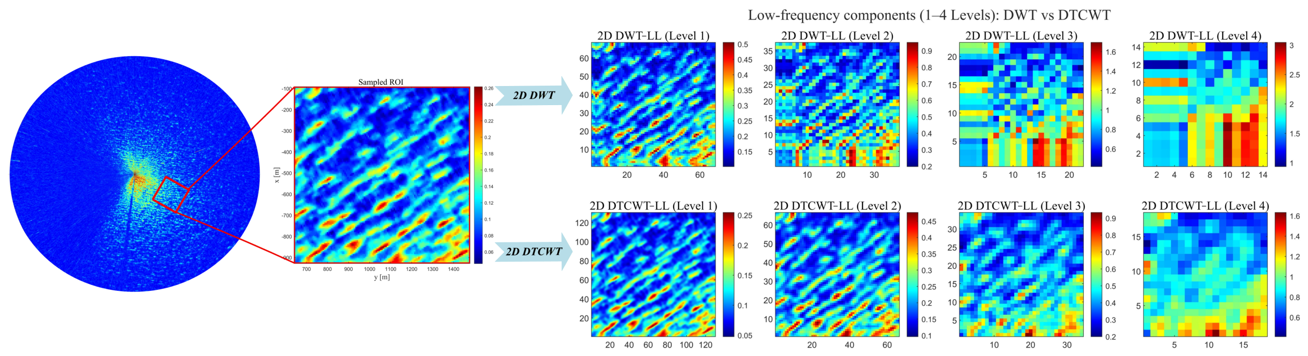
In this study, a 960 m × 960 m region, corresponding to 128 × 128 pixels, is extracted from the original radar image. Both 2D-DWT and 2D-DTCWT are applied at decomposition levels 1 to 4, and the corresponding low-frequency components are shown in Figure 2. The conventional 2D-DWT uses a nonredundant, critically sampled orthogonal filter bank; Thus, at each decomposition level, filtering and downsampling by a factor of 2 along both spatial dimensions reduce the spatial resolution of each subband to one-fourth of that at the preceding level. In contrast, 2D-DTCWT is an overcomplete redundant transform based on dual parallel wavelet trees and approximate Hilbert pairs, providing six-directional selectivity and approximate shift invariance.
As shown in Figure 2, at the same decomposition level, 2D-DTCWT yields smoother and more continuous sea surface streaks with fewer mosaic distortions and spurious artifacts than 2D-DWT. This difference results from their distinct filter-bank structures: 2D-DWT adopts critical downsampling according to the Nyquist sampling criterion, whereas 2D-DTCWT introduces moderate redundancy to improve directional resolution and approximate shift invariance [41]. As the decomposition level increases, the spacing and wavelength of sea surface streaks increase, indicating a gradual reduction in the frequency of the extracted streak features.

2.3. K–Singular Value Decomposition (K-SVD) Dictionary Learning

K-SVD has been widely used in image denoising [42] and fault detection [43], demonstrating strong dictionary-learning capability. Unlike wavelet-based methods with fixed transform bases, K-SVD learns image-adaptive dictionaries and can generate sparse representations suitable for target enhancement and feature extraction in radar images.
In this study, orthogonal matching pursuit (OMP) is combined with K-SVD dictionary learning within a CSC framework to construct a sparse representation model. The model extracts low-frequency basis components and smooth structural information while suppressing high-frequency textures, random noise, and interfering targets through sparsity constraints. For marine radar images, the learned atoms are used to characterize wind energy distributions and improve wind direction retrieval.
Given a training data matrix Y R n × N , whose columns are N training samples, K-SVD learns an overcomplete dictionary D R n × K with K > n and the sparse coefficient matrix X R K × N . The training data are approximated as
Y D X .
The K-SVD optimization problem is formulated as [44]
min D , X Y D X F 2 s . t . x i 0 T 0 .
where x i is the i-th column of X , · F denotes the Frobenius norm, · 0 denotes the l 0 pseudo-norm, and T 0 is the maximum sparsity level.
Since (14) is nonconvex, K-SVD adopts alternating optimization. It first estimates X for a fixed D through sparse coding and then updates the atoms of D while preserving the sparsity pattern of X .

2.3.1. Sparse Coding Stage

With D fixed, the sparse representation of each training sample y i , i = 1 , 2 , , N , is estimated using OMP:
x ^ i = arg min x i y i D x i 2 2 , s . t . x i 0 T 0 .
OMP greedily selects the atom most correlated with the current residual, updates the support set, and computes the coefficients by least-squares projection. At the t-th iteration, the selected atom index is
k = arg max k d k , r ( t 1 ) ,
where d k is the k-th atom of D , and r ( t 1 ) is the residual from the previous iteration. The process stops when T 0 is reached or the reconstruction error falls below a preset threshold.

2.3.2. Dictionary Update Stage

After sparse coding, K-SVD updates D atom by atom. For the k-th atom d k and its coefficient row x k , : , the residual excluding d k is
E k = Y m k d m x m , : .
To preserve the sparsity pattern, only samples using d k are involved in the update. Their index set is
ω k = i x k , : ( i ) 0 .
Using ω k , E k and x k , : are restricted to the active samples, yielding the reduced residual matrix E k R .
Singular value decomposition (SVD) is then performed:
E k R = U Σ V T .
According to the best rank-one approximation, the atom and its nonzero coefficients are updated as
d k = u 1 ,
and
x k , : R = σ 1 v 1 T ,
where σ 1 is the largest singular value, and u 1 and v 1 are the first left and right singular vectors, respectively.
The sparse coding and dictionary update stages are repeated until the maximum number of iterations is reached or the objective function converges.

2.4. Convolutional Sparse Coding (CSC)

Convolutional sparse coding (CSC) represents images using a limited set of spatially shiftable convolutional kernels. Its shift-invariant structure enables local feature extraction while assigning random noise and anomalous components to the residual term under sparsity constraints. CSC has been applied to seismic, medical, radar, and ultrasound wavefield data, where it can recover physical target signals under strong noise [45] and adaptively decompose images with multiple structural components using customized kernels [46].
To suppress interference in marine radar images under complex sea conditions, this study uses CSC to extract and reconstruct wind-field signals. Unlike conventional sparse representation methods that require image segmentation and may disrupt large-scale spatial continuity, CSC performs global optimization over the entire image. By using the wind-signal dictionary learned by K-SVD as convolutional kernels, CSC preserves the spatial distribution of wind-related signals and suppresses sea clutter and interfering targets, such as waves and vessels.
Let S R H × W denote the preprocessed marine radar image, where H and W are the image height and width, respectively. Given the K-SVD-learned convolutional filter set F = { f k } k = 1 K , with f k R n × n , the CSC model is expressed as
S = k = 1 K f k Z k + E ,
where ∗ denotes two-dimensional convolution, Z k R H × W is the sparse feature map corresponding to the k-th filter, and E R H × W represents the reconstruction residual or additive noise.
The sparse feature maps are obtained by solving [47]
Z ^ k k = 1 K = arg min { Z k } k = 1 K 1 2 S k = 1 K f k Z k F 2 + λ k = 1 K Z k 1 .
Here, f k represents a typical local wind-related pattern, and Z k gives its spatial activation map. The parameter λ > 0 balances reconstruction fidelity and sparsity: a larger λ produces sparser maps but may suppress details, whereas a smaller λ preserves details but may introduce redundant responses. The first term in (23) enforces reconstruction accuracy, and the second term promotes sparse activations. Thus, CSC represents complex wind-field structures using a limited number of significant feature responses.

3. Algorithm

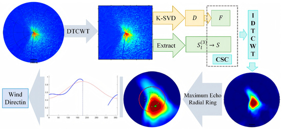
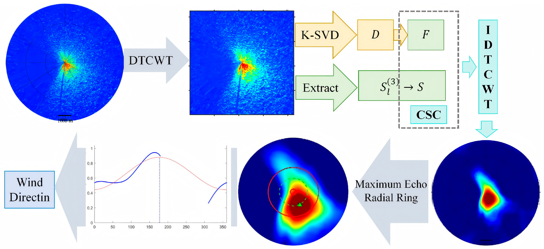
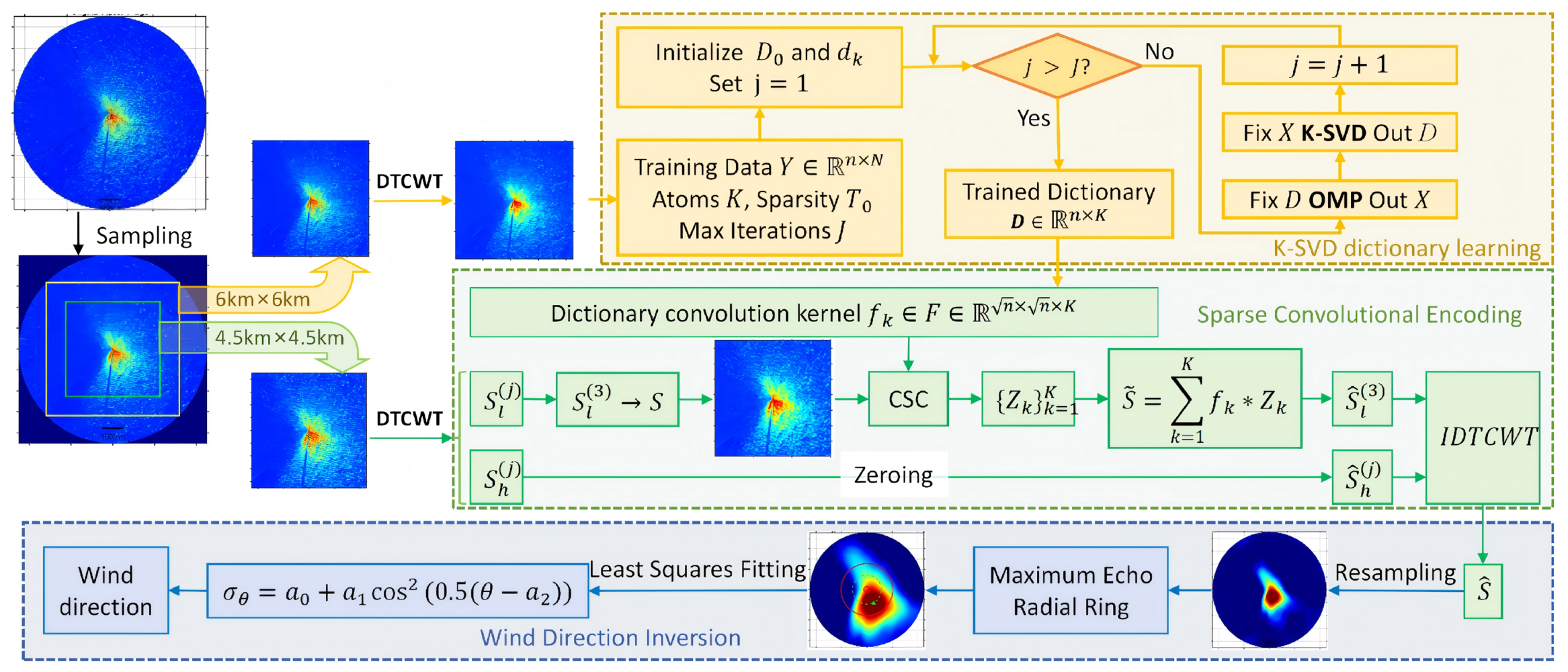
The overall workflow is shown in Figure 3. First, the radar image is resampled in Cartesian coordinates, and the inscribed-square region is selected for dictionary learning. Dictionary learning is performed using an image-wise adaptive strategy rather than by pre-training a fixed global dictionary from all radar images; therefore, a supervised training–test split is not required. For each radar image to be processed, a three-level 2D-DTCWT is first applied, and image patches extracted from the resulting low-frequency component are used as samples for dictionary learning. After 2D-DTCWT decomposition, the extracted samples are used to train an OMP-based K-SVD model. The sparse coefficient matrix X and dictionary atoms D are iteratively updated to learn wind signal features. The learned atoms are then reshaped and column-wise normalized in column-major order to generate a three-dimensional convolutional kernel tensor F .
Next, a square region of size 6000 m × 6000 m ( 800 × 800 pixels), centered on the sampling area, is selected as the dictionary-learning region and subjected to three-level 2D-DTCWT decomposition. This suppresses high-frequency noise and reduces the computational burden in the wavelet domain. For CSC, a central square region of size 4500 m × 4500 m ( 600 × 600 pixels) is selected. The learned kernel tensor F is applied to the low-frequency image components for CSC, yielding sparse feature response maps { Z k } k = 1 K . The distribution image of wind energy is then reconstructed from F and { Z k } k = 1 K , producing S ^ , which retains the low-frequency energy characteristics of the wind signal.
By setting the high-frequency coefficients to zero and applying IDTCWT, the distribution of wind energy is mapped from the wavelet domain back to the physical spatial domain. Finally, S ^ is resampled in polar coordinates, and the effective echo fitting region is determined using the maximum-energy radial ring method. Within this region, the echo intensity and azimuth are fitted using a least-squares cosine-squared model to obtain the final wind direction retrieval result.
Overall, the proposed method forms a two-stage filtering framework. The first stage performs signal separation in the wavelet domain, whereas the second stage conducts learning-based wind energy extraction and effective radial ring selection. This design addresses both frequency-directional mixing and spatial nonuniformity in X-band marine radar images.

3.1. 2D-DTCWT

Marine radar images mainly contain four signal components: white noise, sea waves, targets, and wind modulation. Since this study focuses on wind direction retrieval, all components other than wind modulation are treated as interference. According to their spatial scales, scale-dependent filtering can suppress part of this interference and enhance wind modulation signals. White noise has a spatial scale of no more than several meters [48] and is mainly represented as high-frequency components after 2D-DTCWT decomposition. Wave signals have wavelengths of 60 m to 150 m [49] and correspond to mid- to high-frequency components. Wind-modulated signals occur at scales of several hundred meters [50] and are close to quasi-static components, while sea-surface targets exhibit step responses [51]. Therefore, wind-modulated sea surface streaks can be regarded as low-frequency signals.
As discussed in Section 2, the extracted signal frequency decreases as the number of 2D-DTCWT decomposition levels increases. After three-level 2D-DTCWT decomposition, the image resolution changes from 7.5 m to 60 m , approximately 1/8 to 1/4 of the scale of small-scale wind streaks [32]. At this scale, wind-streak echoes masked by ocean-wave components enhance the echo intensity in the wind direction. Therefore, three-level 2D-DTCWT decomposition is selected for wind direction retrieval.
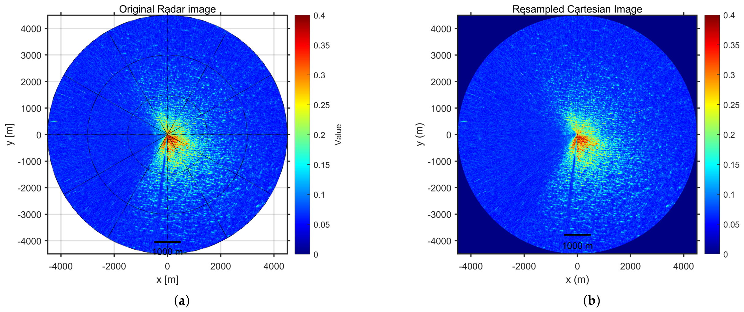
To reduce the influence of low signal-to-noise ratios far from the image center and ensure consistency with subsequent CSC processing, the original radar image with a spatial resolution of 7.5 m is resampled in Cartesian coordinates. The sampling intervals in the horizontal and vertical directions are set to Δ x = Δ y = 7.5 m , producing a 1200 × 1200 -pixel image. The original and resampled radar images are shown in Figure 4a,b.
For the sampled radar images, a central region with a radial extent of 3000 m is processed using three-level 2D-DWT and 2D-DTCWT decompositions. The corresponding low-frequency reconstructed images are shown in Figure 5a,b. Both methods preserve the overall energy distribution and large-scale background of radar echoes, but differ in their representation of low-frequency ripple information. Due to critical downsampling and limited directional selectivity, 2D-DWT weakens the continuity of low-frequency texture ripples and introduces patch-like artifacts. In contrast, 2D-DTCWT provides stronger directional selectivity and approximate shift invariance, producing smoother boundaries, more coherent slowly varying ripples, and more concentrated energy distributions. Thus, 2D-DTCWT provides a more robust low-frequency representation for subsequent wind parameter retrieval and reduces interference from high-frequency white noise and mid- to high-frequency wave noise.

3.2. K-SVD Convolution Kernels

This study employs K-SVD to learn convolutional kernels in the low-frequency wind signal space obtained after 2D-DTCWT decomposition. Unlike manually designed filters or fixed statistical windows, the learned kernels capture representative wind energy distribution patterns from radar images and improve the adaptability of wind signal extraction.

3.2.1. Training-Patch Preparation and Problem Formulation

For images processed by full-frame 2D-DTCWT decomposition, N patches are extracted from the central region for dictionary learning. The patch size affects the learned dictionary: small patches emphasize fine details, whereas large patches require more training samples. Considering that wind modulation is a quasi-static component in radar echoes, each patch should cover at least four to five wavelengths of wind energy. After three-level 2D-DTCWT decomposition, the physical resolution becomes 7.5 m × 4 = 30 m . Therefore, the patch size is set to 32 × 32 , corresponding to 960 m × 960 m .
An overcomplete dictionary is used to represent diverse structural features. Although K is commonly set to two to four times the signal dimension, increasing K also increases overfitting risk and computational cost. As shown in Figure 6, increasing K from 1024 to 2048 provides only marginal reduction in reconstruction error. Therefore, K = 1024 is selected to balance representation capacity and computational efficiency.
The number of training patches N should be much larger than K, typically within 10 K to 40 K , to avoid overfitting. In this study, N = 20 , 000 patches are selected from the radial region within 400 pixels, corresponding to 3000 m , from the image center. Specifically, 20 , 000 patches of size 32 × 32 are randomly cropped, vectorized, and stacked column-wise to form the training matrix Y R n × N , where n = 32 × 32 and N = 20 , 000 . The patches are mean-centered to make dictionary learning focus on texture variation rather than patch brightness.
The sparsity level T 0 controls the number of atoms used to represent each sample. A smaller T 0 improves noise robustness but may cause underfitting. Since wind energy distributions are low-frequency and spatially correlated, most energy trends can be represented by a few atoms; therefore, T 0 = 5 is used.
The K-SVD training process was evaluated under wind speeds from 10 m / s to 14 m / s . As shown in Figure 6, the reconstruction error decreases rapidly within the first 10 iterations and reaches a plateau after 30 iterations. Further iterations reduce Y D X F by less than 0.1 % . Thus, the maximum iteration number is set to J = 30 .

3.2.2. K-SVD Dictionary Learning

In this study, K-SVD dictionary learning is performed using an image-wise adaptive strategy rather than by pre-training a fixed global dictionary from all radar images. For each radar image to be processed, a three-level 2D-DTCWT decomposition is first performed, and image patches are extracted from the corresponding low-frequency component as training samples. Subsequently, these image patches are vectorized to form the training matrix Y , and the wind-signal dictionary D corresponding to the current image is learned using OMP-based K-SVD. Consequently, the dictionaries learned from different radar images are not necessarily identical, and they are primarily used to characterize the low-frequency wind-energy distribution in the current image. It should be noted that the reference wind direction measured by the anemometer is not used during dictionary learning and is used solely to evaluate the accuracy of the final retrieval results.
An initial dictionary D 0 R n × K is constructed, where n is the atom dimension and K is the number of atoms. Each atom d k is initialized from N ( 0 , 1 ) and normalized as
d k d k d k 2 , k = 1 , 2 , , K .
This normalization removes scale ambiguity between dictionary atoms and sparse coefficients and improves sparse coding stability.
The K-SVD dictionary learning workflow is shown in Figure 7. It alternates between OMP-based sparse coding and atom-wise dictionary updating.
Step 1: Sparse Coding Stage (OMP).
Given D 0 , OMP computes the sparse coefficient vector x i for each sample y i Y . It iteratively selects the atom most correlated with the current residual and updates the coefficients by projection onto the selected atom subspace. The process stops when x i contains at most T 0 nonzero elements. The sparse coefficient matrix is then formed as X = [ x 1 , x 2 , , x N ] R K × N . The sparsity constraint suppresses high-frequency noise responses and provides atom-activation information for dictionary updating.
Step 2: Dictionary Update Stage (K-SVD).
Given X , each dictionary atom is updated sequentially. For the k-th atom d k , the algorithm identifies samples using this atom, removes the contributions of other atoms, and constructs the restricted residual matrix E k R . Singular value decomposition (SVD) is then applied to E k R . The atom is updated using the first left singular vector u 1 , and the corresponding sparse coefficients are updated as x R k δ 1 v 1 T . This atom-wise update over the corresponding support set helps reduce the overall reconstruction error.
Step 3: Error Calculation.
OMP sparse coding and K-SVD dictionary updating are repeated until the reconstruction error falls below a preset threshold or the maximum iteration number J is reached. The final dictionary atoms provide sparse linear representations of all training samples.

3.2.3. 3D Convolution Kernel Generation

The learned dictionary matrix D R n × K contains K atoms, where n is the vectorized atom dimension and n × n is the spatial size of each convolutional kernel. The k-th column d k R n corresponds to the vectorized form of the k-th kernel. For two-dimensional convolutional computation, D is reshaped in column-major order into a three-dimensional tensor F = { f k } k = 1 K R n × n × K .
To ensure scale consistency and numerical stability, each kernel slice in F is normalized by the Frobenius norm:
F : , : , k F : , : , k F : , : , k F , k = 1 , , K ,
where · F denotes the Frobenius norm. After normalization, all convolutional kernels have unit Frobenius norm, preventing response bias caused by differences in kernel magnitude. The resulting tensor F can be directly applied to the input image for CSC.

3.3. CSC

Using the K-SVD algorithm, a convolutional kernel tensor F = { f k } k = 1 K R n × n × K containing local morphological features of the wind field is obtained. To extract wind-direction-related signals from a marine radar image S , which is affected by complex sea conditions and contains superimposed wave echoes, target echoes, and noise, this study introduces a global convolutional sparse coding method to reconstruct the wind-signal energy distribution, thereby enabling spatial localization of wind-direction-related energy. It should be noted that the CSC stage does not involve any additional training; instead, it directly solves for the sparse feature response maps { Z k } k = 1 K corresponding to the current radar image, given the convolutional kernel tensor F learned using K-SVD, and then reconstructs the wind-signal energy distribution through convolution. Because CSC performs joint optimization over the entire image without requiring block-wise decomposition and reassembly, it preserves the large-scale continuity of the wind signal, reduces the influence of local wave textures, target echoes, and random noise, and provides a more stable energy-distribution basis for subsequent maximum-energy radial-ring selection.
The raw radar image is fully sampled at intervals of 7.5 m in both horizontal and vertical directions, producing a 1200 × 1200 image matrix. To maintain consistency with the comparison algorithm, the central 800 × 800 region is selected. To reduce convolutional computation, three-level 2D-DTCWT decomposition is applied in the complex wavelet domain, yielding the low-frequency component S l ( j ) and high-frequency component S h ( j ) at each level. The third-level low-frequency component S l ( 3 ) is selected as the experimental input image S R 200 × 200 .
Unlike image-block sparse representation methods, CSC performs joint optimization over the entire image S using convolutional kernels f k . The sparse feature response maps { Z k } k = 1 K are obtained by solving the optimization problem in (22), and the reconstructed wind field image S ˜ R 200 × 200 is synthesized as
S ˜ = k = 1 K f k Z k ,
where f k denotes the k-th convolutional kernel, Z k is the corresponding sparse feature response map, and ∗ denotes convolution.
Because CSC operates on the full image without block partitioning or reassembly, Z k acts as a spatial response index and preserves the spatial distribution and intensity gradients of wind field signals. The shift invariance of the convolutional kernels also reduces stitching artifacts and preserves the continuity of large-scale wind streaks and the wind energy distribution.
After CSC-based purification, the remaining high-frequency subband coefficients S h ( j ) are set to zero to obtain S ^ h ( j ) . The CSC-reconstructed low-frequency component S ˜ is assigned to S ^ l ( 3 ) , and the wind energy distribution is mapped back to the spatial pixel domain using IDTCWT:
S ^ = IDTCWT S ^ l ( 3 ) , S ^ h ( j ) .
The final image S ^ R 800 × 800 represents the low-frequency reconstructed wind energy distribution in the radar image. It is then sampled in polar coordinates and restored to the scan-mode echo matrix, with the center of S ^ as the polar origin, a radial sampling interval of 7.5 m , and an angular sampling interval of 0.8 ° . The radial range [ 1 , 300 ] , corresponding to 2250 m , is selected to generate the wind signal energy distribution map, as shown in Figure 8a,b.
With both the raw radar images and dictionary convolutional kernels unit-normalized, λ = 0.02 was adopted as the baseline fixed regularization parameter. As shown in Figure 8a, the conventional CSC model with a globally fixed λ concentrates reconstructed energy near the image center, while wind energy in distant regions nearly vanishes. This occurs because radar echoes undergo range attenuation, making weak signals in distant regions more susceptible to excessive sparsity penalties imposed by a fixed soft threshold. To examine whether the loss of these responses was caused by excessive thresholding, the adaptive interval λ [ 0.0001 , 0.025 ] was empirically constructed by extending the baseline value to a slightly larger upper bound and a near-zero lower bound. Within this interval, λ decreases with radial distance to preserve weak, range-attenuated wind signals while suppressing strong interference. As shown in Figure 8b, adaptive-threshold CSC enhances large-scale wind streaks in the lower-right region while preserving the overall wind energy distribution. Responses that remain negligible when λ approaches 0.0001 are therefore considered to represent genuinely weak wind energy rather than signals eliminated by excessive regularization.

3.4. Wind Direction Retrieval

Echo quality varies with radial distance. Near-range echoes are affected by obstruction, blind zones, and strong clutter, whereas far-range echoes may lose wind direction information because of reduced signal-to-noise ratios. To reduce errors from fixed-radius or full-map statistics, this study fits the azimuthally averaged echo curve within the maximum-energy radial ring, which is selected from the wind energy distribution map.
The maximum-energy location is first identified in the wind energy distribution map. Taking its radial distance as the center, 30 radial samples are extended inward and outward to form a maximum-energy radial ring with a width of 60 samples, corresponding to 450 m . This range covers approximately 1 to 2 wind echo wavelengths, making the averaged echo within the ring more stable. In Figure 9, the region between the two red lines denotes the selected radial band, while the green triangle and green dashed line indicate the maximum-energy location and the corresponding radial ring, respectively.
Within the selected radial ring, the mean echo intensity σ θ is fitted as a function of the azimuth angle θ using the squared cosine model in Equation (1).
The proposed algorithm contains two stages. First, 2D-DTCWT separates low-frequency wind direction modulation signals in the multiscale and multidirectional wavelet domain while suppressing wave textures and radar noise. Second, K-SVD and CSC learn the wind energy distribution in the low-frequency signal space and generate a wind energy response map for maximum-energy radial ring selection. Thus, the method forms a progressive workflow from signal enhancement to region localization, improving wind direction retrieval accuracy.

4. Experimental Results and Analysis

4.1. Experimental Data Sources

The experimental data were obtained from X-band marine radar measurements collected during a sea trial conducted off the coast of Zhejiang, China, in March 2012. The radar antenna was mounted on the forward side of the ship’s main mast, approximately 25 m above sea level. The radar operated in horizontal–horizontal ( HH ) polarization mode, with a range resolution of 7.5 m . With 600 range samples, the coverage radius was approximately 4500 m . The antenna rotation period was 2.5 s , and one radar image was acquired during each rotation. The main radar parameters are listed in Table 1.
The reference wind direction was obtained from an anemometer installed on the same vessel as the X-band marine radar. During the sea trial, the radar antenna was mounted on the forward side of the vessel’s main mast, approximately 25 m above the sea surface, and the anemometer was installed adjacent to the radar antenna. The anemometer provided one wind-speed and wind-direction record per minute. During data acquisition, each radar image was stored together with the concurrent anemometer record, ensuring direct temporal synchronization between the radar and anemometer measurements. The reference wind direction used in this study was the true wind direction expressed in the geographic coordinate system. The anemometer measured wind direction over a range of 0 ° to 360 ° , with an accuracy of ± 3 ° . The main anemometer parameters are listed in Table 2.
The 900-sample main validation dataset was collected under rain-free conditions during vessel navigation off the coast of Zhejiang, China, from 13:47 on 8 March to 08:25 on 9 March 2012, covering 18 h 38 min. The near-blind-zone and away-from-blind-zone validation datasets were each composed of 200 samples selected according to the corresponding wind-direction criteria from a separate rain-free observation period extending from 08:27 to 16:10 on 9 March, covering 7 h 43 min. Therefore, these two datasets do not overlap with the main validation dataset. The 282-sample rainy-condition validation dataset was collected during a rainfall event from 03:41 to 07:39 on 7 March, covering 3 h 58 min.
To further validate the applicability of the proposed method under different environmental conditions, multiple experimental datasets were constructed based on the original sea-trial data. The first dataset served as the main validation dataset and comprised 900 sets of X-band marine radar images and synchronized in situ anemometer wind-direction references, which were used to evaluate the wind-direction retrieval performance of different methods over the entire experimental dataset. With wind speeds mainly ranging from 10 to 16 m/s and reference wind directions mainly ranging from 32 ° to 73 ° .
The second and third datasets were used for blind-zone sensitivity validation to analyze the effect of radar blind zones on wind-direction retrieval results. The near-blind-zone validation dataset contained 200 samples with reference wind directions greater than 50 ° and was used to evaluate the retrieval performance of different methods when the wind direction entered or approached the initial boundary of the radar blind zone. The away-from-blind-zone validation dataset contained 200 samples with reference wind directions less than 50 ° and was used to evaluate the retrieval performance of different methods when the wind direction was away from the radar blind zone. It should be noted that these two 200-sample datasets were additional validation datasets constructed to analyze the effect of radar blind zones and were not subsets derived from the 900-sample main validation dataset.
To evaluate the effect of rainfall on X-band marine radar images, a fourth validation dataset collected under rainy conditions was further added. This dataset includes 282 sets of marine radar images and synchronized in situ anemometer measurements collected under rainy conditions and was used to analyze the robustness of different wind-direction retrieval methods under rain-contaminated conditions.
As shown in Figure 10a,b, the raw radar images were acquired at the same wind speed of 7.8 m/s under rain-free and rainy conditions, respectively. Compared with radar images acquired under rain-free conditions, radar echoes in the rainfall samples are jointly affected by raindrop backscattering, rain-induced attenuation, and nonuniform rain-band distributions; consequently, the images may exhibit large-scale echo enhancement, localized high-intensity patches, or nonuniform rain-band structures. These rain-contamination features alter the echo-intensity distribution and azimuthal energy structure of radar images, thereby affecting wind-direction retrieval results based on azimuthal echo-intensity modulation. Therefore, the rainfall dataset was used separately to validate the robustness of the proposed DTCWT–CSC maximum-energy radial-ring method against rain-contamination interference.
In summary, the experimental data used in this study include 900 main validation samples, 200 near-blind-zone validation samples, 200 away-from-blind-zone validation samples, and 282 rainy condition validation samples. Among these datasets, the main validation dataset was used to evaluate the overall performance of the algorithm; the near-blind-zone and away-from-blind-zone datasets were used to analyze the effect of radar blind zones on the retrieval results; and the rainy-condition dataset was used to analyze the stability of the algorithm under rain-contaminated conditions. Each validation dataset was independent and designed for a specific evaluation purpose.

4.2. Experimental Results

To avoid angular wrap-around errors at the 0 ° / 360 ° boundary, both the radar-retrieved wind direction and the anemometer reference wind direction were first converted into a bow-relative coordinate system, and the angle sequences were unwrapped before calculating the root mean square error (RMSE) and correlation coefficient (CC). Wind-direction errors were calculated using the minimum circular angular difference rather than ordinary linear differences:
e i = mod θ ^ i θ i + 180 ° , 360 ° 180 ° ,
where θ ^ i and θ i denote the radar-retrieved wind direction and anemometer reference wind direction for the i-th sample, respectively, and e i is the corresponding circular angular error, with a range of [ 180 ° , 180 ° ] .
Based on this circular angular error, the mean bias error (MBE) is defined as:
MBE = 1 N i = 1 N e i ,
where MBE < 0 indicates that the retrieval results are generally smaller than the reference wind direction, corresponding to systematic underestimation, whereas MBE > 0 indicates systematic overestimation.
The RMSE is defined as:
RMSE = 1 N i = 1 N e i 2 .
The CC is calculated using the wind-direction sequences after coordinate transformation and angular unwrapping. Let the unwrapped radar-retrieved wind-direction sequence and the reference wind-direction sequence be denoted by θ ^ i c and θ i c , respectively, with mean values θ ^ ¯ c and θ ¯ c . The CC is then defined as:
CC = i = 1 N θ ^ i c θ ^ ¯ c θ i c θ ¯ c i = 1 N θ ^ i c θ ^ ¯ c 2 i = 1 N θ i c θ ¯ c 2 .
This approach prevents angular discontinuities at the 0 ° / 360 ° boundary from affecting the RMSE and CC calculations, thereby ensuring the comparability of evaluation results among different wind-direction retrieval methods.

4.2.1. Overall Retrieval Performance

Figure 4a shows the raw radar image acquired at 21:37 on 8 March 2012. At that time, the ship heading was 225.08 ° , with the radar image referenced to the ship heading. The wind speed was 14.1 m / s , the wind direction was 43.0 ° , and the wind bearing relative to the ship heading was 177.9 ° .
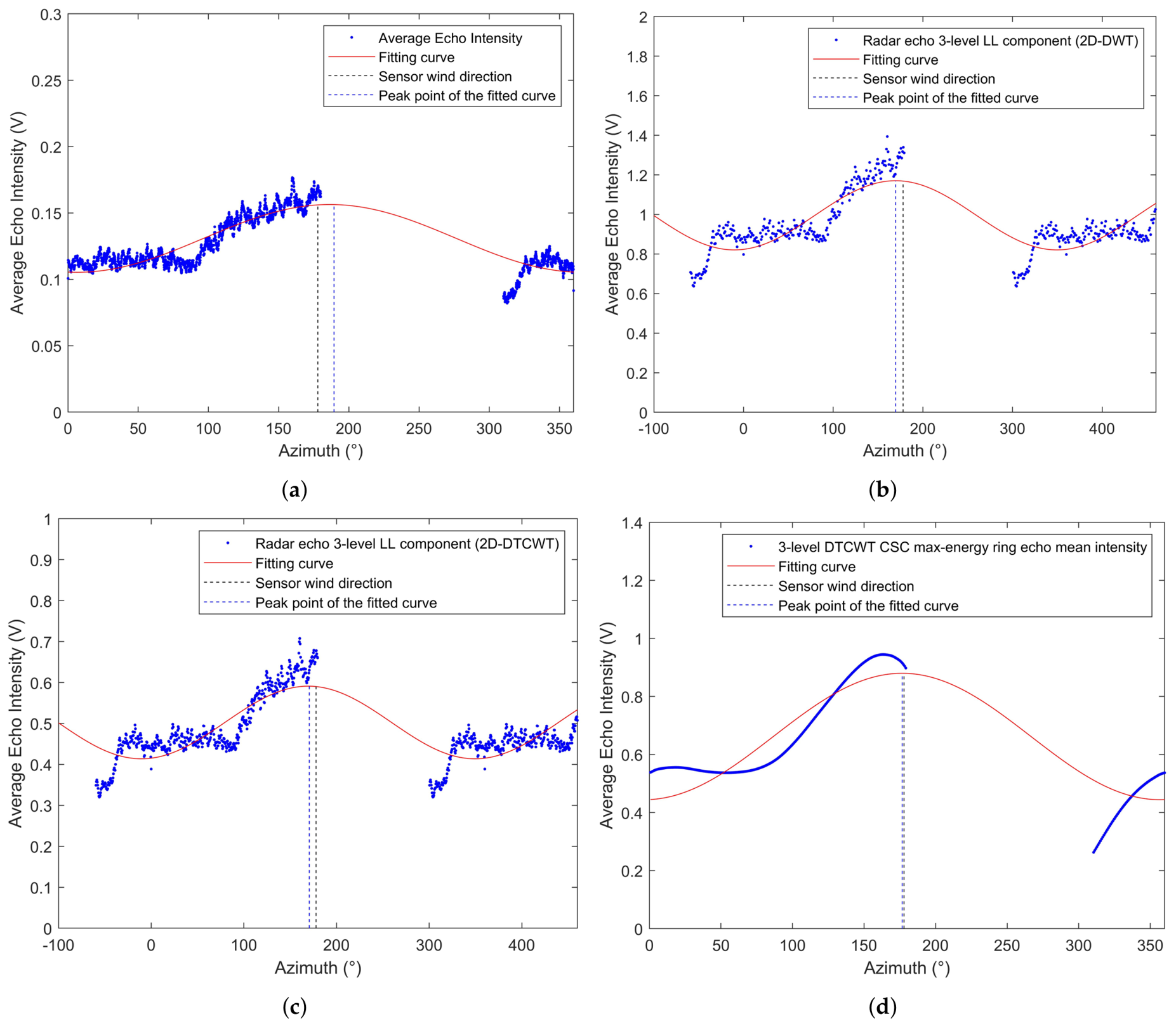
Figure 11 compares the cosine-squared fitting results for echo intensity versus azimuth. The blue scatter points denote the mean echo intensity at each azimuth, calculated over the central radial region within 3000 m , and the red curve denotes the least-squares fitted model. According to the raw radar image, the blind zone caused by the mast and wake was defined as the region from 180 ° to 300 ° relative to the ship bow and was excluded from curve fitting.
Figure 11a shows the fitting result for the transformed raw radar image. The fitted wind direction is 189.5 ° , with an error of 11.6 ° relative to the in situ sensor reference value of 177.9 ° . Figure 11b,c show the results after three-level 2D-DWT and 2D-DTCWT decomposition, respectively. In both cases, the fitting was performed within the central radial region of 3000 m , with the azimuth range extended by 100 ° around the ship bow to avoid discontinuities at the 0 ° / 360 ° boundary. The fitted wind directions are 169.6 ° and 170.7 ° , corresponding to errors of 8.3 ° and 7.2 ° , respectively. These results show that both wavelet transforms suppress noise and extract low-frequency wind signals, while 2D-DTCWT provides slightly more concentrated scatter points and better directional consistency than 2D-DWT.
Figure 11d shows the fitting result obtained within the maximum-energy radial ring after 2D-DTCWT and CSC processing. The retrieved wind direction is 179.5 ° , with an error of 1.6 ° . Compared with the other methods, the echo intensity varies more smoothly with azimuth and exhibits smaller local fluctuations. This indicates that the proposed method preserves the directional advantages of 2D-DTCWT while enhancing the wind energy distribution through CSC, thereby improving azimuthal correlation, fitting stability, and wind direction retrieval accuracy.
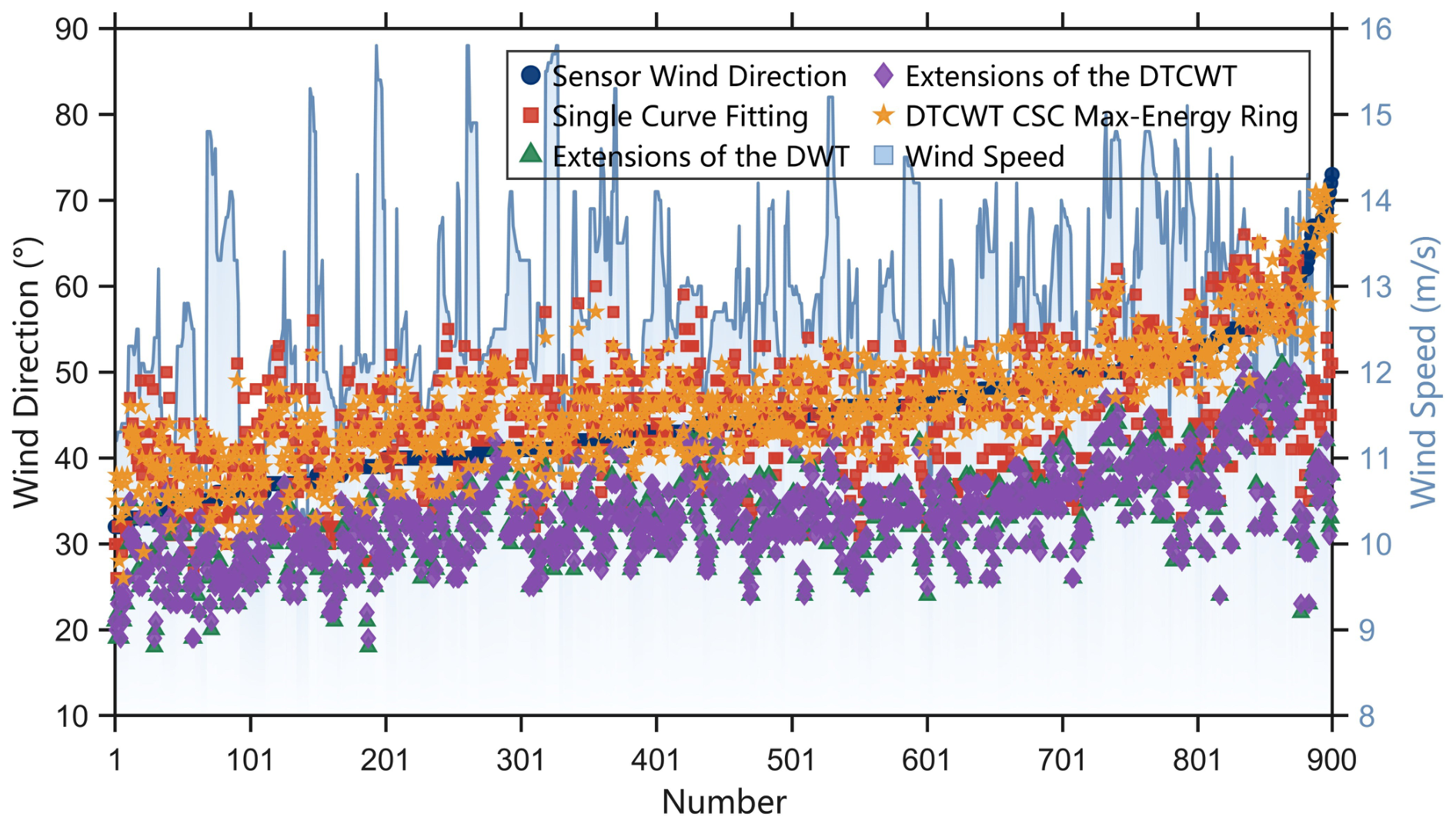
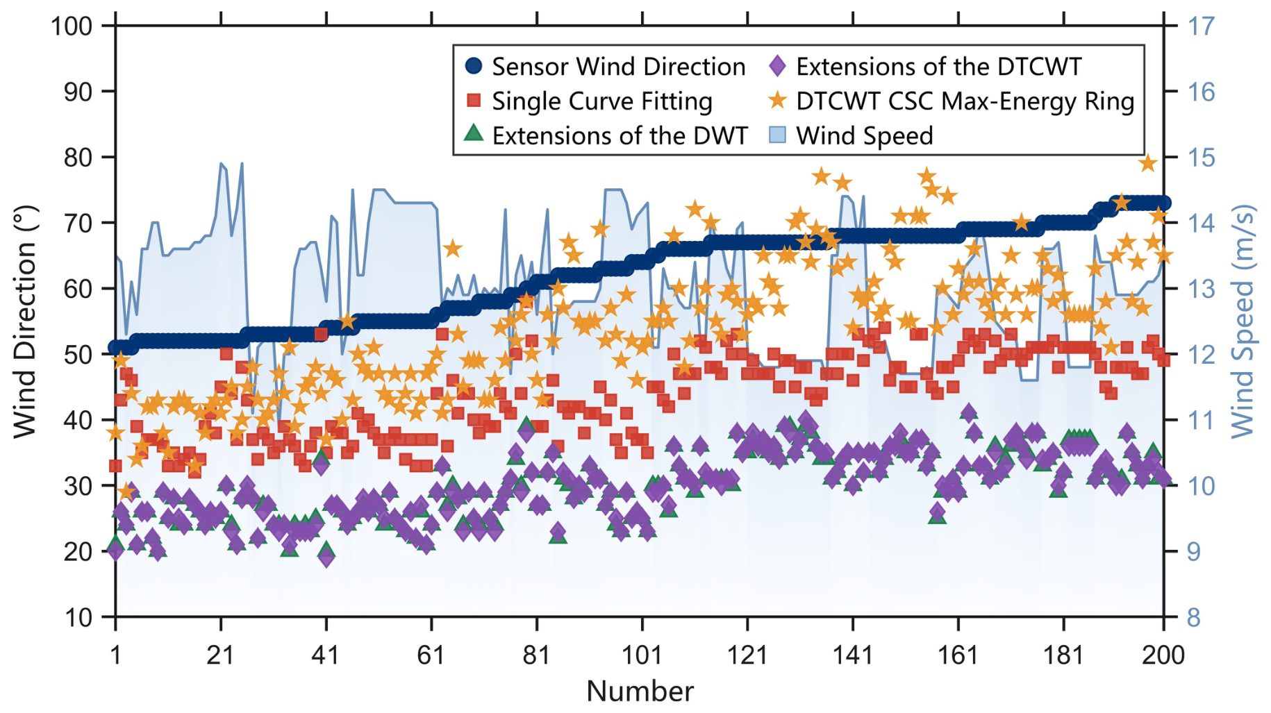
This study compares the experimental results obtained from 900 sets of sea-trial data collected on 8–9 March 2012. The dataset covers wind directions from 32 ° to 73 ° and wind speeds from 10 m / s to 16 m / s , with the ship heading generally maintained at approximately 235 ° . The mast-induced radar blind sector spans relative azimuths of 180 ° 300 ° , corresponding to approximately 55 ° 175 ° in geographic coordinates. Allowing for small variations in ship heading, 50 ° was adopted as a practical threshold near the lower blind-zone boundary: samples above 50 ° were classified as near the blind zone, whereas those below 50 ° were classified as away from it. The scatter plots of the retrieval results obtained by different methods are shown in Figure 12. In all subsequent result figures, the blue data points represent the wind direction reference values measured by the in situ anemometer, and the light blue background indicates wind speed. The red, green, purple, and orange data points represent the wind direction retrieval results obtained using the single-curve fitting method, the extended-bow-heading 2D-DWT method, the extended-bow-heading 2D-DTCWT method, and the proposed 2D-DTCWT–CSC method based on maximum-energy radial rings, respectively. The wind speeds in the experimental dataset range from 10 m / s to 16 m / s , corresponding approximately to Beaufort scale 6–7 winds. Under these conditions, short ocean waves, breaking waves, and wind-induced ripples are pronounced. Thus, the radar images contain not only interference relative to the wind signal but also substantial wind-related characteristic energy, satisfying the complex sea-state conditions required for this study.
As shown by the wind direction retrieval results in Figure 12, the proposed method based on 2D-DTCWT–CSC and maximum-energy radial rings produces results closest to the in situ sensor reference values. The overall trends are highly consistent with the reference data, and the method tracks wind direction effectively even in the later stage, when the wind speed increases rapidly. This verifies the effectiveness of the proposed wind direction feature extraction method.
In contrast, although the results of the single-curve fitting method are generally distributed around the reference values, they exhibit pronounced local fluctuations and clear discontinuities, indicating high sensitivity to anomalous echoes and noise. The 2D-DTCWT method with extended bow heading performs slightly better than the corresponding 2D-DWT method, but both methods generally underestimate the wind direction. This underestimation becomes more evident when the wind direction exceeds approximately 50 ° , because the wind direction then enters the radar blind zone. In addition, third-level low-frequency extraction using 2D-DWT or 2D-DTCWT further increases image-feature blurring, leading to larger retrieval errors.
Within the range of 30 ° to 45 ° , the retrieval results of all methods are relatively close to the in situ anemometer reference values. As the wind direction continues to increase, the retrieval accuracy gradually decreases. This is mainly because data from the blind zone are excluded from the cosine-model fitting, causing the peak of the fitted curve to shift toward the nonblind region and resulting in systematic underestimation of the wind direction.
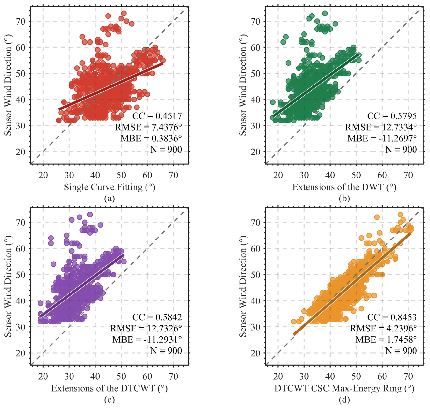
Figure 13 shows the correlation between the wind-direction retrieval results obtained using the four methods and the reference wind-direction values measured by the in situ anemometer for the 900-sample experimental dataset. In Figure 13a, the single-curve fitting method achieves a CC of 0.45, an RMSE of 7.44 ° , and an MBE of 0.38 ° . Although this method has a small mean bias, the scatter points are relatively dispersed, indicating limited capability in tracking wind-direction variations and reduced retrieval stability. In Figure 13b and c, the CC of the extended-bow-heading DWT and DTCWT methods are 0.58, respectively; their RMSEs are 12.73 ° , and their corresponding MBEs are 11.27 ° and 11.29 ° . These results indicate that although both methods exhibit slightly higher correlations than the single-curve fitting method, their retrieval results show significant negative biases, corresponding to systematic underestimation of wind direction and compression of the retrieved wind-direction range.
In contrast, Figure 13d shows that the DTCWT–CSC maximum-energy radial-ring method achieved the best performance, with a CC of 0.85, an RMSE of 4.24 ° , and an MBE of 1.75 ° . The scatter points obtained using this method are closer to the y = x reference line, indicating that its retrieval results agree well with the reference wind direction measured by the in situ anemometer. This improvement can be attributed to the strong directional selectivity of DTCWT, which enables more effective preservation of low-frequency wind-direction modulation features; the ability of CSC to reconstruct the wind-signal energy distribution; and the adaptive selection of effective fitting regions with strong wind-direction-related energy by the maximum-energy radial-ring strategy. Together, these components reduce the influence of wave textures, nonuniform sea clutter, and invalid radial regions on azimuthal fitting.
To further analyze the effect of radar blind zones on wind-direction retrieval accuracy, two additional representative blind-zone sensitivity validation datasets were selected in addition to the 900-sample main validation dataset. The first dataset was the near-blind-zone dataset, which contained 200 samples with reference wind directions greater than 50 ° and was used to analyze the retrieval performance of different methods when the true wind direction entered or approached the initial boundary of the radar blind zone. The second dataset was the away-from-blind-zone dataset, which comprised 200 samples with reference wind directions less than 50 ° and was used to analyze retrieval performance when the wind direction was away from the radar blind zone. It should be noted that these two 200-sample datasets were not subsets extracted from the aforementioned 900-sample main validation dataset; rather, they were additional validation datasets specifically constructed to analyze the effect of radar blind zones.

4.2.2. Retrieval Performance near the Blind Zone

To investigate the effect of proximity to the blind zone on the wind direction retrieval performance of each method, 200 additional experiments were conducted. The anemometer reference wind direction of 50 ° , corresponding to the starting angle of the blind zone, was used as the boundary for grouping the experimental data.
Figure 14 and Figure 15 show the retrieval results when the anemometer reference wind direction exceeds 50 ° , i.e., when the true wind direction enters or approaches the starting angle of the radar blind zone. Compared with the full-dataset results, the errors of all methods increase markedly under this condition, indicating that blind-zone effects substantially degrade the accuracy of wind direction retrieval from marine radar images.
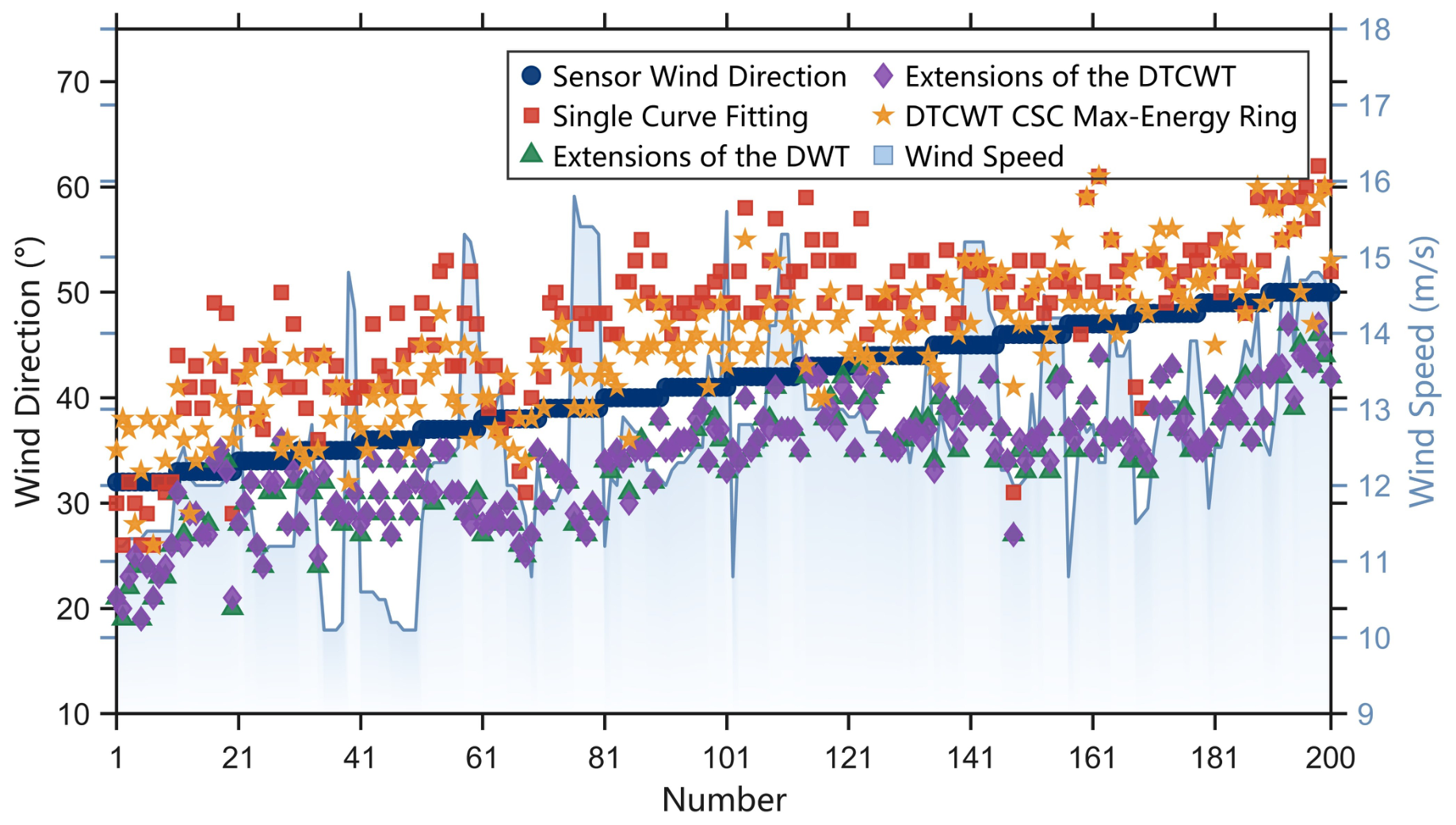
As shown in Figure 14, the reference wind direction of the 200 samples gradually increases from 50 ° to 73 ° , while the wind speed is mainly concentrated between 10 m / s and 15 m / s , corresponding to moderate-to-high wind speed conditions. Therefore, the reduction in retrieval accuracy is not primarily caused by weak echo characteristics at low wind speeds, but is mainly related to the loss of wind-induced textures, blurred image features, and incomplete energy distributions caused by the radar blind zone.
The performance varies markedly among the different methods. The retrieval results of the single-curve fitting method are mainly concentrated between 35 ° and 55 ° . Although they increase slightly with the reference wind direction, their dynamic range is narrow, indicating limited tracking capability, especially when the reference wind direction exceeds 60 ° . The extended-bow-heading 2D-DWT and 2D-DTCWT methods are more strongly affected by the blind zone, with retrieval results mainly concentrated between 20 ° and 40 ° , showing clear systematic underestimation. This indicates that conventional wavelet extension methods have difficulty extracting the prevailing wind direction from incomplete radar images.
In contrast, the proposed method based on 2D-DTCWT–CSC and maximum-energy radial rings achieves the best overall performance. Its retrieval results are mainly distributed between 40 ° and 80 ° , showing good tracking of the wind direction changes measured by the sensor, particularly as the wind direction approaches the blind zone. However, compared with the full-sample results, this method still exhibits increased dispersion, indicating that the blind zone continues to reduce the stability of directional feature extraction.
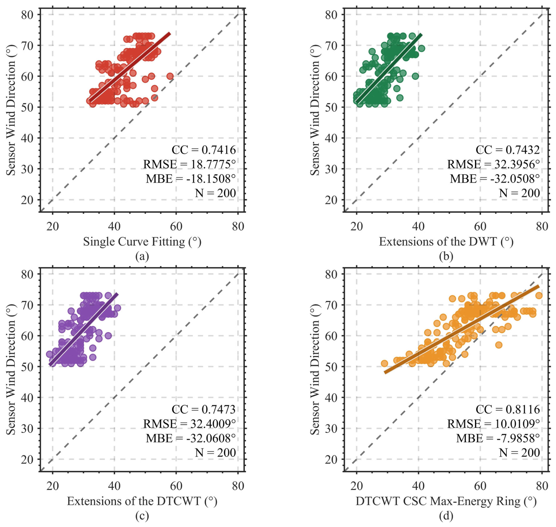
Figure 15 further illustrates the correlation and error metrics of the four methods under near-blind-zone conditions. The single-curve fitting method achieved a CC of 0.74, an RMSE of 18.78 ° , and an MBE of 18.15 ° , indicating that although this method could follow the overall trend of the reference wind direction to some extent, its retrieval results exhibited significant systematic underestimation. The CCs of the extended-bow-heading DWT and DTCWT methods were 0.74 and 0.75, respectively; however, their RMSEs reached 32.40 ° and 32.40 ° , with corresponding MBEs of 32.05 ° and 32.06 ° . As shown by the scatter distributions, the data points of both methods were almost entirely located above the y = x reference line, indicating that the sensor-measured wind directions were substantially greater than the radar-retrieved wind directions and thus demonstrating pronounced underestimation. These results suggest that although the extended-bow-heading DWT and DTCWT methods still retained some monotonic correlation, their retrieval results deviated substantially from the reference values; therefore, they are unsuitable for wind-direction retrieval when the wind direction enters or approaches the radar blind zone.
Under near-blind-zone conditions, the DTCWT–CSC maximum-energy radial-ring method achieved the best performance, with CC, RMSE, and MBE values of 0.81, 10.01 ° , and 7.99 ° , respectively. Compared with the extended-bow-heading 2D-DWT and 2D-DTCWT methods, the proposed method substantially reduced the RMSE, and the absolute MBE decreased from approximately 32 ° to 8 ° , indicating that it effectively mitigates systematic underestimation. These results show that when the true wind direction enters or approaches the radar blind zone, occlusion disrupts the low-frequency wind-induced texture and directional energy distribution, making traditional fixed-region or extended-bow-heading fitting methods more susceptible to residual wave textures, nonuniform sea clutter, and occlusion-edge echoes. These interferences shift the fitted peak toward smaller azimuth angles. By combining DTCWT-based texture suppression, CSC-based wind-energy reconstruction, and maximum-energy radial-ring selection, the proposed method reduces the influence of invalid radial regions and residual blind-zone echoes. Overall, radar blind zones introduce both random disturbances and directional systematic biases; the extended-bow-heading 2D-DWT and 2D-DTCWT methods are most affected, followed by the single-curve fitting method, whereas the proposed method shows the strongest resistance to occlusion, although its retrieval accuracy still decreases in this region.

4.2.3. Retrieval Performance Away from Blind Zone

To further analyze the influence of the blind zone, this study selected 200 samples for which the anemometer reference wind direction was less than 50 ° . The results are shown in Figure 16 and Figure 17. Compared with conditions near the blind zone, the retrieval accuracy of all methods improves markedly, indicating that the blind zone is a key factor affecting wind direction retrieval from marine radar images.
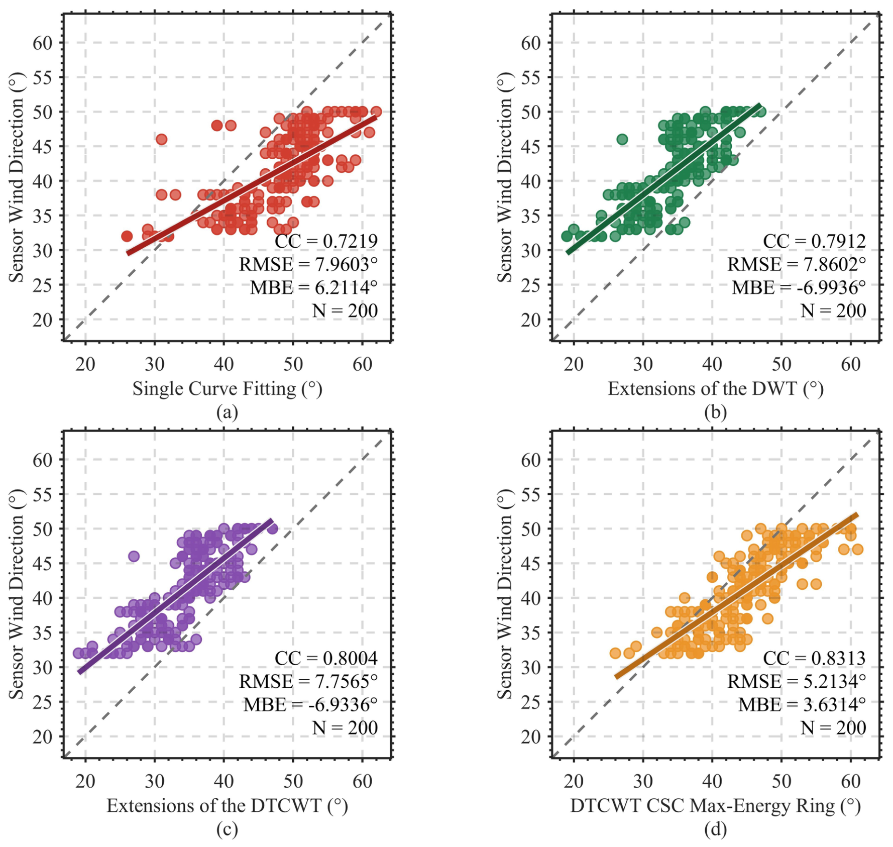
In Figure 16, away from the blind zone, all four methods can effectively track changes in the sensor-measured wind direction. The single-curve fitting method captures the overall trend but exhibits clear local fluctuations. The 2D-DWT method shows substantial improvement compared with its performance near the blind zone, but remains relatively sensitive to occlusion. The 2D-DTCWT method produces more concentrated scatter points and shows better stability than 2D-DWT. In comparison, the proposed method based on 2D-DTCWT–CSC and maximum-energy radial rings achieves the best performance, with retrieval results closest to the anemometer reference values. This indicates that the proposed method can extract dominant wind direction information more accurately and stably.
As shown in Figure 17, when the reference wind direction is away from the radar blind zone, the retrieval performance of all methods improves significantly. The single-curve fitting, extended-bow-heading 2D-DWT, extended-bow-heading 2D-DTCWT, and DTCWT–CSC maximum-energy radial-ring methods achieved CC values of 0.72, 0.79, 0.80, and 0.83, respectively; RMSEs of 7.96 ° , 7.86 ° , 7.76 ° , and 5.21 ° ; and MBEs of 6.21 ° , 6.9936 ° , 6.93 ° , and 3.63 ° . Compared with the near-blind-zone results, the RMSEs of all methods decreased significantly. This improvement was particularly evident for the extended-bow-heading 2D-DWT and 2D-DTCWT methods, for which the RMSE decreased from approximately 32 ° to 8 ° , and the absolute MBE decreased from approximately 32 ° to 7 ° . This indicates that when the wind direction is away from the radar blind zone, the low-frequency wind-induced textures and azimuthal energy distribution in the radar image are more completely preserved. Consequently, more effective azimuthal information is available for curve fitting, and the fitted peak is closer to the reference wind direction, thereby significantly reducing systematic bias.
In contrast, the DTCWT–CSC maximum-energy radial-ring method still achieved the best performance under away-from-blind-zone conditions, with CC, RMSE, and MBE values of 0.83, 5.21 ° , and 3.63 ° , respectively. Combined with the near-blind-zone results, the proposed method maintained relatively low RMSE and MBE values under both blind-zone conditions. This indicates that it can mitigate the influence of blind-zone occlusion, nonuniform sea clutter, and local anomalous echoes on azimuthal fitting through the directional selectivity of DTCWT, the wind-energy reconstruction capability of CSC, and effective-region selection using the maximum-energy radial-ring strategy. These results further demonstrate that the systematic underestimation observed near the blind zone is primarily caused by radar blind-zone occlusion rather than by wind-speed variations or random noise alone.
The wind speeds in both experimental datasets were mainly concentrated between 10 m / s and 16 m / s , indicating that wind speed was not the dominant factor causing the observed error differences. Instead, the retrieval performance was primarily affected by whether the wind direction fell within the blind-zone-sensitive region. When the wind direction was away from the blind zone, the effective wind-induced textures in the radar images were relatively complete, enabling the extraction of sufficient directional information. In contrast, when the wind direction was close to the blind zone, some dominant textures were occluded or weakened, causing conventional methods to extract local directional features that deviated from the true wind direction. The proposed 2D-DTCWT–CSC method based on maximum-energy radial rings achieved the lowest RMSE under both conditions, demonstrating stronger robustness and higher accuracy in wind direction retrieval.
It should be noted that all methods in this study used the same bow-heading correction and coordinate transformation procedures. Radar images were first transformed into relative azimuth coordinates using the ship bow as the reference, and the geographic wind direction measured by the anemometer was converted into the bow-relative wind direction based on the simultaneously recorded ship heading. Therefore, the effects of bow-heading correction and coordinate transformation were consistent across the four methods. If the systematic errors were primarily caused by bow-heading correction or coordinate transformation, the four methods would be expected to exhibit approximately consistent overall angular offsets. However, the experimental results show that the extended-bow-heading 2D-DWT and 2D-DTCWT methods produced significant negative biases of approximately 32 ° under near-blind-zone conditions, whereas the negative bias of the proposed method was reduced to 7.99 ° . This indicates that the primary source of systematic underestimation was not coordinate transformation or bow-heading correction, but rather the effect of the radar blind zone on the ability of different methods to extract wind-direction features.
In addition, fitting-region selection can contribute to systematic bias. Traditional methods typically compute echo-intensity statistics within a fixed radial region or an extended bow-heading azimuth region. When the dominant wind-direction texture is partially occluded by the radar blind zone, the azimuthal energy distribution within the selected region may be affected by local wave textures, nonuniform sea clutter, and residual echoes near the obstruction edges, which can shift the fitted-curve peak away from the true wind direction. In the proposed method, CSC is used to reconstruct the wind-signal energy distribution, and the maximum-energy radial-ring strategy is employed to adaptively select regions with relatively strong wind-related energy. This design reduces the influence of invalid radial regions and residual blind-zone echoes on azimuthal fitting, thereby alleviating systematic underestimation under blind-zone conditions.

4.2.4. Retrieval Performance Under Rainy Conditions

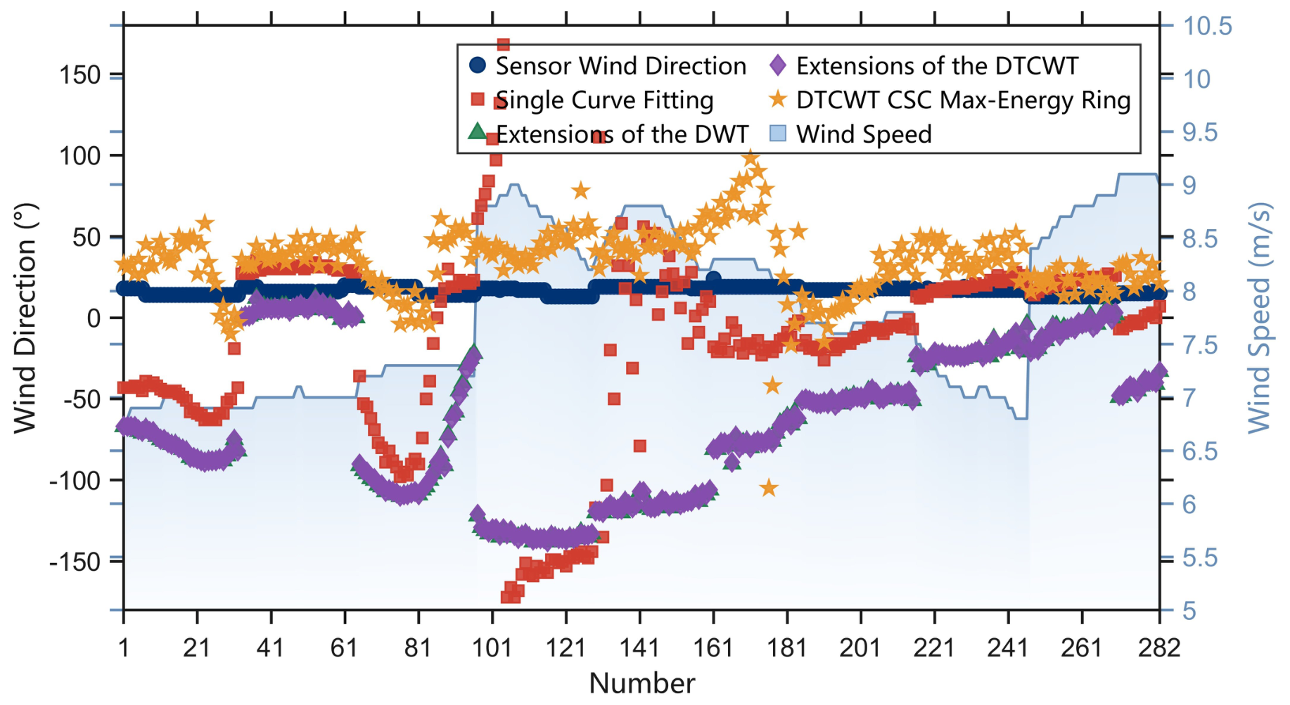
Figure 18 shows the wind-direction retrieval results of the four methods under rainy conditions. The time-series comparison shows that, under rainy conditions, the reference wind direction measured by the in situ anemometer remained relatively stable overall, whereas the radar-based retrieval results of the four methods exhibited varying degrees of fluctuations and biases. The single-curve fitting method exhibited noticeable discrete jumps during several periods, whereas the extended-bow-heading 2D-DWT and 2D-DTCWT methods showed pronounced negative biases over extended intervals. These results suggest that rain-contaminated echoes can substantially disturb the low-frequency wind-induced textures and azimuthal energy distribution in radar images, thereby reducing the reliability of traditional wind-direction retrieval methods based on azimuthal echo-intensity statistics.
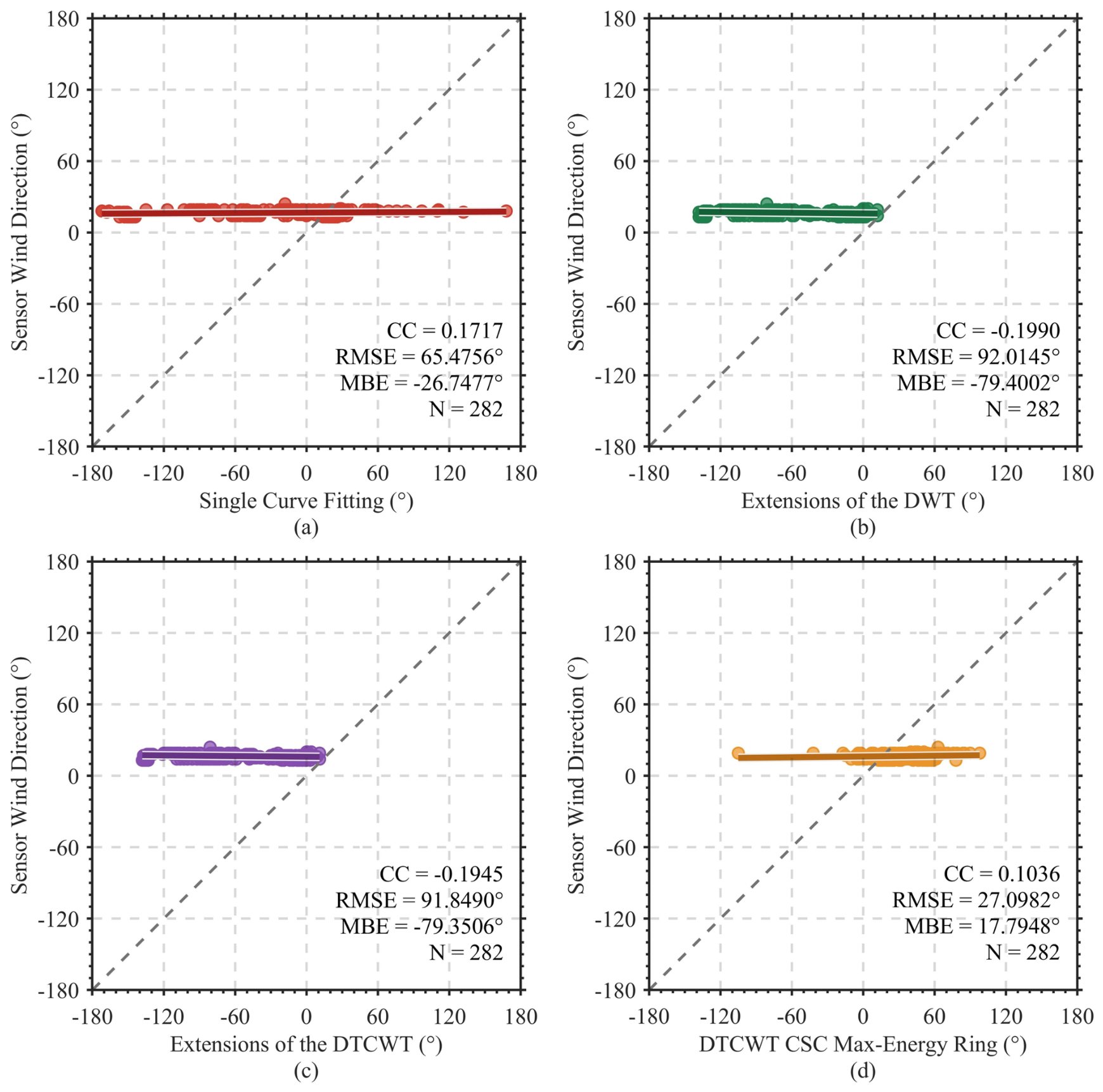
Figure 19 further presents the CC and error metrics of the four methods under rainy conditions. The single-curve fitting method achieved a CC of 0.17, an RMSE of 65.48 ° , and an MBE of 26.75 ° , indicating that its retrieval results under rainy conditions were highly dispersed and showed marked underestimation. The extended-bow-heading 2D-DWT and 2D-DTCWT methods were more severely affected by rain contamination, with CC values of 0.20 and 0.19 , RMSEs of 92.01 ° and 91.85 ° , and MBEs of 79.40 ° and 79.35 ° , respectively. These results suggest that, under rainy conditions, raindrop scattering, rain-induced attenuation, and nonuniform rain-band echoes can alter the overall intensity distribution of radar images. Consequently, wind-direction modulation information in the low-frequency components may be disturbed or partially masked by rain clutter, leading to substantial deviations in the azimuthal fitting results.
In contrast, the DTCWT–CSC maximum-energy radial-ring method still exhibited relatively low errors under rainy conditions, with CC, RMSE, and MBE values of 0.10, 27.10 ° , and 17.80 ° , respectively. Compared with the other three methods, the proposed method reduced anomalous deviations caused by rain contamination to some extent, suggesting that the directional selectivity of DTCWT, the sparse energy reconstruction capability of CSC, and effective-region selection using the maximum-energy radial-ring strategy contributed to the partial suppression of rain-clutter interference. However, the CC of this method under rainy conditions remained low, and the RMSE still exceeded 27 ° , indicating that the current wind-direction retrieval procedure alone is insufficient to fully eliminate the influence of rainfall on X-band marine radar images.
Therefore, experimental results under rainfall conditions indicate that rain contamination significantly reduces the reliability of wind-induced texture and azimuthal energy features in radar images, and may cause the regions of maximum energy to be dominated by echoes from rain bands, thereby affecting subsequent curve fitting and wind direction estimation. Although the method described in this paper still outperforms the comparison methods in rainfall samples, its inversion accuracy does not yet meet the requirements for stable wind measurement. Consequently, when performing wind direction inversion using X-band maritime radar under actual rainfall conditions, professional rain contamination detection, rain area removal, or rain clutter filtering should be performed first, followed by wind direction inversion. Future research will combine rainfall identification and rain clutter suppression algorithms to further improve the applicability and robustness of the proposed method under rainy navigation conditions.

4.2.5. Overall Performance Comparison

The statistical results are summarized in Table 3. In the full-sample experiments, the single-curve fitting method yields the lowest correlation coefficient because it fits the overall echo-intensity curve and is therefore sensitive to local noise, nonuniform sea clutter, and texture loss caused by the blind zone. When wind-induced streaks are discontinuous or the local energy distribution is distorted, the fitted curve tends to deviate from the true prevailing wind direction.
The correlation coefficients of the extended-bow-heading 2D-DWT and 2D-DTCWT methods are slightly higher than that of the single-curve fitting method, but they remain relatively low, and their RMSE values are large. This is mainly caused by systematic underestimation rather than random errors. The wind directions retrieved by both methods are generally lower than the anemometer reference values, indicating compression of their directional response range. This phenomenon is particularly evident when the true wind direction approaches the blind zone, where the dominant wind texture is obscured or weakened. As a result, the wavelet-based methods tend to misinterpret the local energy direction in the visible region as the true wind direction.
Using 2D-DTCWT with extended bow heading alone provides only limited improvement over 2D-DWT. This indicates that the main limitation of conventional methods lies not only in wavelet decomposition itself but also in the lack of robust selection of effective wind signal regions.
In contrast, the proposed method combines the directional selectivity of 2D-DTCWT, the energy localization capability of CSC, and the maximum-energy radial ring constraint, enabling more reliable identification of the prevailing wind direction. For the full dataset, samples near the blind zone, and samples far from the blind zone, the proposed method achieves the lowest RMSE values of 4.24 ° , 10.01 ° , and 5.21 ° , respectively. These results indicate that the proposed method has stronger directional feature extraction capability and greater robustness to blind-zone occlusion, making it more suitable for wind direction retrieval from marine radar images under complex sea conditions. However, the wind-direction retrieval accuracy under rainy conditions evaluated in this study still requires further investigation and improvement.


5. Conclusions

This study developed a wind direction retrieval method based on 2D-DTCWT–CSC and maximum-energy radial rings using X-band marine radar images acquired under moderate-to-high wind speed conditions. By suppressing wave textures and nonuniform sea clutter while aggregating low-frequency directional energy across the radar images, the proposed method enhances the extraction of wind-induced modulation signals. The performance of the proposed method was evaluated against that of the single-curve fitting method, the extended-bow-heading 2D-DWT method, and the extended-bow-heading 2D-DTCWT method.
On the main validation dataset, the proposed method achieved the highest CC, at 0.85, and the lowest RMSE, at 4.24 ° . By comparison, the single-curve fitting method yielded a CC of 0.45 and an RMSE of 7.44 ° , whereas the two extended-bow-heading wavelet methods both yielded CCs of approximately 0.58 and RMSEs of approximately 12.73 ° . These results correspond to RMSE reductions of 43.0% compared with the single-curve fitting method and 66.7% compared with each of the two extended-bow-heading wavelet methods. Although the single-curve fitting method yielded the lowest MBE, at 0.38 ° , its substantially lower CC and higher RMSE indicate a weaker ability to accurately track variations in wind direction. The comparable performance of the extended-bow-heading 2D-DWT and 2D-DTCWT methods further indicates that replacing 2D-DWT with 2D-DTCWT alone provides little improvement, underscoring the importance of integrating 2D-DTCWT with CSC and maximum-energy radial rings.
The influence of the blind zone was evaluated by dividing the experiments into near-blind-zone and away-from-blind-zone groups according to the angular separation between the reference wind direction and the blind zone, with 50 ° used as the grouping threshold. When the wind direction was away from the blind zone, the proposed method achieved a CC of 0.8313 and an RMSE of 5.21 ° , representing RMSE reductions ranging from 32.8% to 34.5% compared with the three benchmark methods. When the wind direction was close to the blind zone, the dominant directional textures and associated energy distributions were disrupted, leading to systematic underestimation and larger retrieval errors across all four methods. Under this condition, the RMSEs of the extended-bow-heading 2D-DWT and 2D-DTCWT methods increased to approximately 32.4 ° , whereas the proposed method still achieved a CC of 0.81 and an RMSE of 10.01 ° . Compared with the single-curve fitting method, the proposed method reduced the RMSE by 46.7%; compared with each of the two extended-bow-heading wavelet methods, it reduced the RMSE by approximately 69.1%. Nevertheless, the MBE of the proposed method shifted from a positive bias of 3.63 ° away from the blind zone to a negative bias of 7.99 ° near the blind zone, indicating that the method mitigates, but does not completely eliminate, blind-zone interference.
Under rainy conditions, the proposed method yielded an RMSE of 27.10 ° , substantially lower than the range of 65.48 ° to 92.01 ° obtained using the benchmark methods. However, all four methods exhibited low or negative CCs, indicating that none of them reliably captured variations in wind direction under rainfall interference. Overall, the proposed method demonstrated higher retrieval accuracy and greater robustness than the benchmark methods under non-rainy, moderate-to-high wind speed conditions, particularly when the wind direction was near the radar blind zone. However, the validation data were primarily concentrated within the wind speed range of 10 to 16 m s 1 ; consequently, the performance of the proposed method under low wind speeds, extreme gales, and rainfall interference remains to be established. Future work will expand the dataset to encompass a wider range of environmental conditions and refine the blind-zone correction and dominant-direction extraction procedures, thereby enhancing the generalizability of marine radar-based wind direction retrieval.

Author Contributions

Conceptualization, J.X.; data curation, Z.L.; funding acquisition, H.W. and Z.L.; methodology, J.X. and B.W.; software, J.X.; validation, J.X., Z.L., H.W. and Y.W.; writing—original draft preparation, J.X.; writing—review and editing, J.X. All authors have read and agreed to the published version of the manuscript.

Funding

This work was supported by the Natural Science Foundation of Guangdong Province (Youth Enhancement Program, Grant No. 2024A1515030159), the Guangzhou Basic and Applied Basic Research Program—Youth Doctoral “Qihang” Project (Grant No. SL2024A04J01461), the Guangdong Provincial Key Fields Special Project for Regular Universities (Grant No. 2024ZDZX3038), the Research Capacity Enhancement Project for Key Developing Disciplines in Guangdong Province (Grant No. 2025ZDJS123), and Young Scientists Fund of the National Natural Science Foundation of China (Grant Nos. 41906154 and 52101358).

Data Availability Statement

The data presented in this study are available on request from Zhizhong Lu.

Acknowledgments

The authors would like to thank the two anonymous reviewers for their valuable comments and suggestions.

Conflicts of Interest

The authors declare no conflicts of interest.

References

  1. Baleani, C.A.; Menendez, M.C.; Vitale, A.J.; Amodeo, M.R.; Perillo, G.M.E.; Piccolo, M.C. Assessing the role of tidal cycle, waves, and wind as drivers of surf zone zooplankton on a temperate sandy beach. Reg. Stud. Mar. Sci. 2024, 73, 103455. [Google Scholar] [CrossRef] [Scilit]
  2. Yang, Z.; Huang, W.; Chen, X. Mitigation of rain effect on wave height measurement using X-band radar sensor. IEEE Sens. J. 2022, 22, 5929–5938. [Google Scholar] [CrossRef] [Scilit]
  3. Zhang, Y.; Liu, F.; Lu, Z.; Wei, Y.; Wang, H. Multi-anemometer optimal layout and weighted fusion method for estimation of ship surface steady-state wind parameters. Ocean Eng. 2022, 266, 112793. [Google Scholar] [CrossRef] [Scilit]
  4. Huang, W.; Liu, X.; Gill, E.W. Ocean wind and wave measurements using X-band marine radar: A comprehensive review. Remote Sens. 2017, 9, 1261. [Google Scholar] [CrossRef] [Scilit]
  5. Kahma, K.K. On errors in wind speed observations on R/V Aranda. Geophysica 1981, 17, 155–165. [Google Scholar]
  6. Blanc, T.V. Superstructure Flow Distortion Corrections for Wind Speed and Direction Measurements Made from Tarawa Class (LHA1-LHA5) Ships; Technical Report; U.S. Naval Research Laboratory: Washington, DC, USA, 1986.
  7. Polsky, S.; Ghee, T.; Butler, J.; Czerwiec, R. Application of CFD to anemometer position evaluation: A feasibility study. In Proceedings of the 29th AIAA Applied Aerodynamics Conference; American Institute of Aeronautics and Astronautics: Reston, VA, USA, 2011; p. 3346. [Google Scholar]
  8. Landwehr, S.; O’Sullivan, N.; Ward, B. Direct flux measurements from mobile platforms at sea: Motion and airflow distortion corrections revisited. J. Atmos. Ocean. Technol. 2015, 32, 1163–1178. [Google Scholar] [CrossRef] [Scilit]
  9. Thornhill, E.; Wall, A.; McTavish, S.; Lee, R. Ship anemometer bias management. Ocean Eng. 2020, 216, 107843. [Google Scholar] [CrossRef] [Scilit]
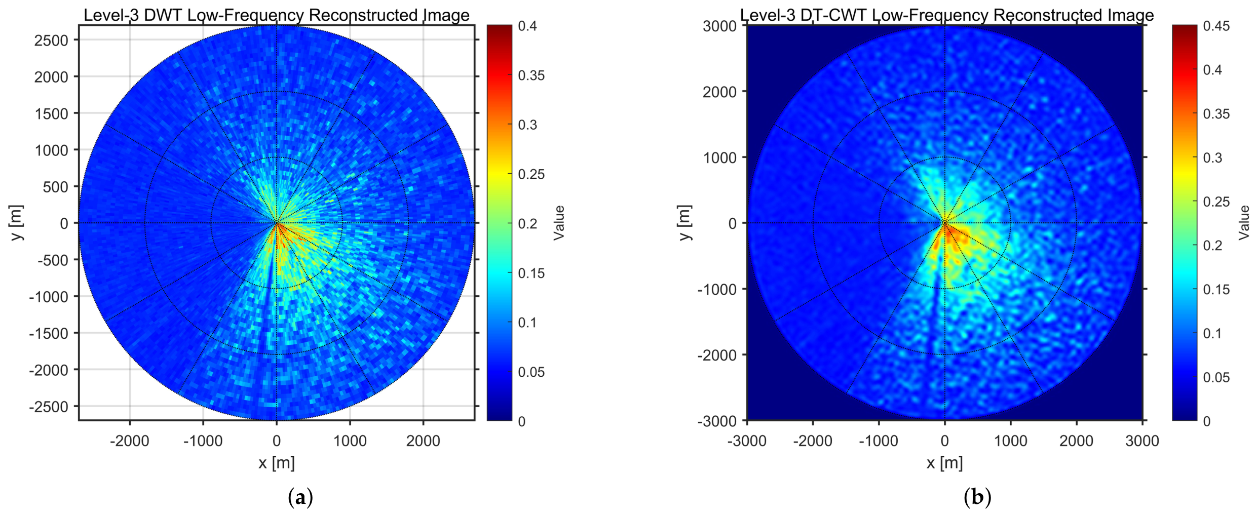
  10. Ni, W.; Stoffelen, A.; Ren, K. Tropical cyclone wind direction retrieval from dual-polarized SAR imagery using histogram of oriented gradients and Hann window function. IEEE J. Sel. Top. Appl. Earth Obs. Remote Sens. 2022, 16, 878–888. [Google Scholar] [CrossRef] [Scilit]
  11. Huang, W.; Gill, E.; Wu, X.; Li, L. Measurement of sea surface wind direction using bistatic high-frequency radar. IEEE Trans. Geosci. Remote Sens. 2012, 50, 4117–4122. [Google Scholar] [CrossRef] [Scilit]
  12. Huang, W.; Wu, S.; Gill, E.; Wen, B.; Hou, J. HF radar wave and wind measurement over the Eastern China Sea. IEEE Trans. Geosci. Remote Sens. 2002, 40, 1950–1955. [Google Scholar] [CrossRef]
  13. Zhao, C.; Chen, Z.; He, C.; Xie, F.; Chen, X. A hybrid beam-forming and direction-finding method for wind direction sensing based on HF radar. IEEE Trans. Geosci. Remote Sens. 2018, 56, 6622–6629. [Google Scholar] [CrossRef] [Scilit]
  14. Ijima, T.; Takahashi, T.; Sasaki, H. Application of radars to wave observations. Coast. Eng. Proc. 1964, 30, 10–22. [Google Scholar]
  15. Liu, Y.; Huang, W.; Gill, E.W.; Peters, D.K.; Vicen-Bueno, R. Comparison of algorithms for wind parameters extraction from shipborne X-band marine radar images. IEEE J. Sel. Top. Appl. Earth Obs. Remote Sens. 2014, 8, 896–906. [Google Scholar] [CrossRef] [Scilit]
  16. Yang, Z.; Huang, W. WSTCNN: A wavelet scattering transform-CNN model for wind speed estimation from radar images. IEEE Trans. Geosci. Remote Sens. 2025, 63, 5105813. [Google Scholar] [CrossRef] [Scilit]
  17. Dankert, H.; Horstmann, J. A marine radar wind sensor. J. Atmos. Ocean. Technol. 2007, 24, 1629–1642. [Google Scholar] [CrossRef] [Scilit]
  18. Dankert, H.; Horstmann, J.; Koch, W.; Rosenthal, W. Ocean wind fields retrieved from radar-image sequences. In Proceedings of the IEEE International Geoscience and Remote Sensing Symposium; IEEE: Piscataway, NJ, USA, 2002; Volume 4, pp. 2150–2152. [Google Scholar]
  19. Dankert, H.; Horstmann, J.; Rosenthal, W. Wind-and wave-field measurements using marine X-band radar-image sequences. IEEE J. Ocean. Eng. 2005, 30, 534–542. [Google Scholar] [CrossRef] [Scilit]
  20. Wang, H.; Lu, Z. Research on Small Scale Wind Streak Factor of Navigation Radar-Image Sequences. In Proceedings of the 2015 8th International Symposium on Computational Intelligence and Design (ISCID); IEEE: Piscataway, NJ, USA, 2015; Volume 1, pp. 335–339. [Google Scholar]
  21. Wang, H.; Qiu, H.; Lu, Z.; Wang, L.; Akhtar, R.; Wei, Y. An energy spectrum algorithm for wind direction retrieval from X-band marine radar image sequences. IEEE J. Sel. Top. Appl. Earth Obs. Remote Sens. 2021, 14, 4074–4088. [Google Scholar] [CrossRef] [Scilit]
  22. Wang, H.; Li, S.; Qiu, H.; Lu, Z.; Wei, Y.; Zhu, Z.; Ge, H. Development of a fast convergence gray-level co-occurrence matrix for sea surface wind direction extraction from marine radar images. Remote Sens. 2023, 15, 2078. [Google Scholar] [CrossRef] [Scilit]
  23. Hatten, H.; Seemann, J.; Horstmann, J.; Ziemer, F. Azimuthal dependence of the radar cross section and the spectral background noise of a nautical radar at grazing incidence. In Proceedings of the IGARSS’98. Sensing and Managing the Environment. 1998 IEEE International Geoscience and Remote Sensing. Symposium Proceedings. (Cat. No. 98CH36174); IEEE: Piscataway, NJ, USA, 1998; Volume 5, pp. 2490–2492. [Google Scholar]
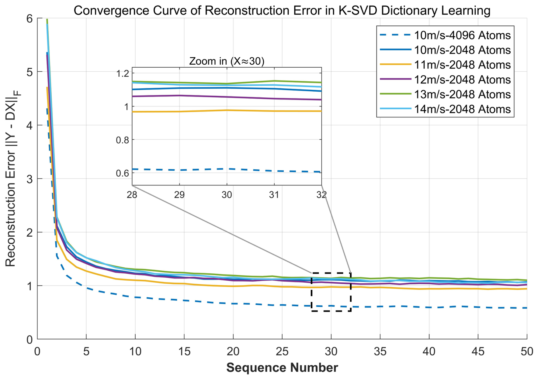
  24. Lund, B.; Graber, H.C.; Romeiser, R. Wind retrieval from shipborne nautical X-band radar data. IEEE Trans. Geosci. Remote Sens. 2012, 50, 3800–3811. [Google Scholar] [CrossRef] [Scilit]
  25. Liu, Y.; Huang, W.; Gill, E.W.; Peters, D.K. Dual-curve-fitting-based wind parameter extraction from shipborne nautical X-band radar data. In Proceedings of the OCEANS 2014-TAIPEI; IEEE: Piscataway, NJ, USA, 2014; pp. 1–5. [Google Scholar]
  26. Chen, Z.; He, Y.; Zhang, B.; Qiu, Z. Determination of nearshore sea surface wind vector from marine X-band radar images. Ocean Eng. 2015, 96, 79–85. [Google Scholar] [CrossRef] [Scilit]
  27. Chen, X.; Huang, W. Identification of rain and low-backscatter regions in X-band marine radar images: An unsupervised approach. IEEE Trans. Geosci. Remote Sens. 2020, 58, 4225–4236. [Google Scholar] [CrossRef] [Scilit]
  28. Chen, X.; Huang, W.; Zhao, C.; Tian, Y. Rain detection from X-band marine radar images: A support vector machine-based approach. IEEE Trans. Geosci. Remote Sens. 2019, 58, 2115–2123. [Google Scholar] [CrossRef] [Scilit]
  29. Wang, Y.; Huang, W. An algorithm for wind direction retrieval from X-band marine radar images. IEEE Geosci. Remote Sens. Lett. 2016, 13, 252–256. [Google Scholar] [CrossRef] [Scilit]
  30. Huang, W.; Liu, Y.; Gill, E.W. Texture-analysis-incorporated wind parameters extraction from rain-contaminated X-band nautical radar images. Remote Sens. 2017, 9, 166. [Google Scholar] [CrossRef] [Scilit]
  31. Liu, X.; Huang, W.; Gill, E.W. Wind direction estimation from rain-contaminated marine radar data using the ensemble empirical mode decomposition method. IEEE Trans. Geosci. Remote Sens. 2016, 55, 1833–1841. [Google Scholar] [CrossRef] [Scilit]
  32. Yu, H.; Wang, H.; Lu, Z. Wind-Direction Estimation from Single X-Band Marine Radar Image Improvement by Utilizing the DWT and Azimuth-Scale Expansion Method. Entropy 2022, 24, 747. [Google Scholar] [CrossRef] [Scilit] [PubMed]
  33. Li, S.; Yang, B.; Hu, J. Performance comparison of different multi-resolution transforms for image fusion. Inf. Fusion 2011, 12, 74–84. [Google Scholar] [CrossRef] [Scilit]
  34. Liu, Y.; Chen, X.; Wang, Z.; Wang, Z.J.; Ward, R.K.; Wang, X. Deep learning for pixel-level image fusion: Recent advances and future prospects. Inf. Fusion 2018, 42, 158–173. [Google Scholar] [CrossRef] [Scilit]
  35. Ranjani, J.J.; Thiruvengadam, S. Dual-tree complex wavelet transform based SAR despeckling using interscale dependence. IEEE Trans. Geosci. Remote Sens. 2010, 48, 2723–2731. [Google Scholar] [CrossRef] [Scilit]
  36. Shi, W.; Zhu, C.; Tian, Y.; Nichol, J. Wavelet-based image fusion and quality assessment. Int. J. Appl. Earth Obs. Geoinf. 2005, 6, 241–251. [Google Scholar] [CrossRef] [Scilit]
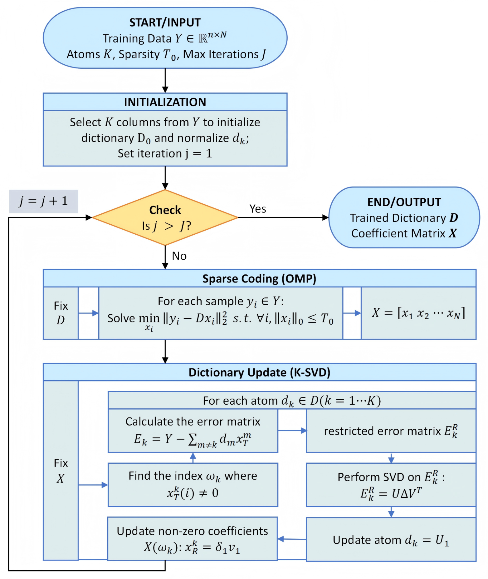
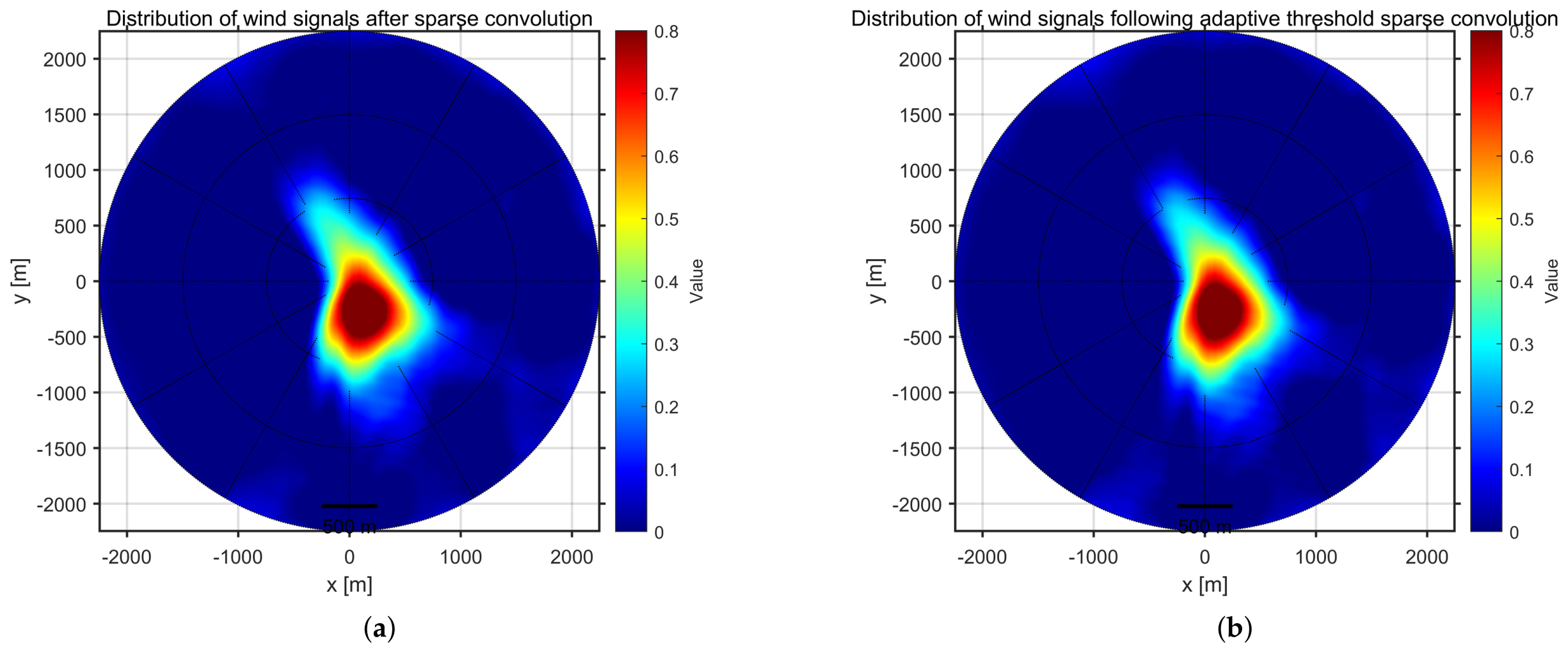
  37. He, Z.; Guo, Z.; Wang, L.; Yang, G.; Diao, Y.; Ma, D. WaveGuard: Robust Deepfake Detection and Source Tracing via Dual-Tree Complex Wavelet and Graph Neural Networks. IEEE Trans. Circuits Syst. Video Technol. 2025, 36, 4757–4770. [Google Scholar] [CrossRef] [Scilit]
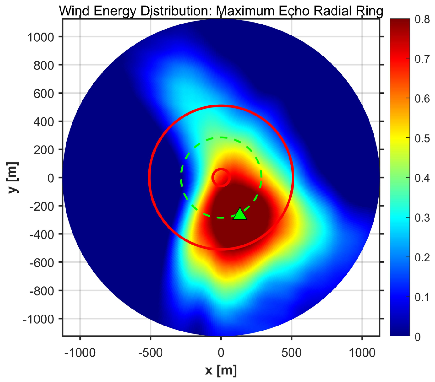
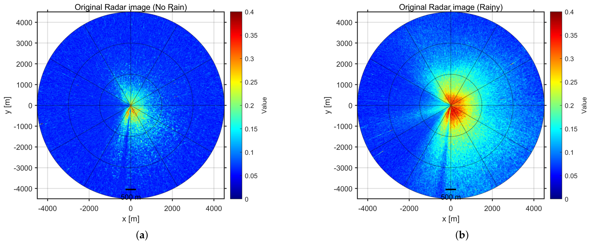
  38. Igbineweka, E.; Chowdhury, S. Application of dual-tree complex wavelet transform in islanding detection for a hybrid AC/DC microgrid with multiple distributed generators. Energies 2024, 17, 5133. [Google Scholar] [CrossRef] [Scilit]
  39. Selesnick, I.W.; Baraniuk, R.G.; Kingsbury, N.C. The dual-tree complex wavelet transform. IEEE Signal Process. Mag. 2005, 22, 123–151. [Google Scholar] [CrossRef] [Scilit]
  40. Yu, R. Theory of dual-tree complex wavelets. IEEE Trans. Signal Process. 2008, 56, 4263–4273. [Google Scholar] [CrossRef] [Scilit]
  41. Yang, J.; Wang, Y.; Xu, W.; Dai, Q. Image and video denoising using adaptive dual-tree discrete wavelet packets. IEEE Trans. Circuits Syst. Video Technol. 2009, 19, 642–655. [Google Scholar] [CrossRef] [Scilit]
  42. Ye, W.; Li, S.; Zhao, X.; Abubakar, A.; Bermak, A. AK times singular value decomposition based image denoising algorithm for DoFP polarization image sensors with Gaussian noise. IEEE Sens. J. 2018, 18, 6138–6144. [Google Scholar] [CrossRef] [Scilit]
  43. Edun, A.S.; LaFlamme, C.; Kingston, S.R.; Tetali, H.V.; Benoit, E.J.; Scarpulla, M.; Furse, C.M.; Harley, J.B. Finding faults in PV systems: Supervised and unsupervised dictionary learning with SSTDR. IEEE Sens. J. 2020, 21, 4855–4865. [Google Scholar] [CrossRef] [Scilit]
  44. Aharon, M.; Elad, M.; Bruckstein, A. K-SVD: An algorithm for designing overcomplete dictionaries for sparse representation. IEEE Trans. Signal Process. 2006, 54, 4311–4322. [Google Scholar] [CrossRef] [Scilit]
  45. Pereg, D.; Cohen, I.; Vassiliou, A.A. Convolutional sparse coding fast approximation with application to seismic reflectivity estimation. IEEE Trans. Geosci. Remote Sens. 2021, 60, 5905819. [Google Scholar] [CrossRef] [Scilit]
  46. Zhang, H.; Patel, V.M. Convolutional Sparse Coding-based Image Decomposition. In Proceedings of the BMVC; Rutgers University: New Brunswick, NJ, USA, 2016. [Google Scholar]
  47. Zeiler, M.D.; Krishnan, D.; Taylor, G.W.; Fergus, R. Deconvolutional networks. In Proceedings of the 2010 IEEE Computer Society Conference on Computer Vision and Pattern Recognition; IEEE Computer Society: Los Alamitos, CA, USA, 2010; pp. 2528–2535. [Google Scholar]
  48. Jun, H.; Min, Y.; Park, S.H.; Kim, N.H.; Jeong, J.Y.; Lee, S.C.; Do, K. Enhanced Calibration of Miros Wave and Current Radar Using a Deep Neural Network at Sochengcho Ocean Research Station, Korea. J. Atmos. Ocean. Technol. 2025, 42, 369–386. [Google Scholar] [CrossRef] [Scilit]
  49. Grigorieva, V.; Badulin, S.; Gulev, S. Global validation of SWIM/CFOSAT wind waves against voluntary observing ship data. Earth Space Sci. 2022, 9, e2021EA002008. [Google Scholar] [CrossRef] [Scilit]
  50. Dankert, H.; Horstmann, J.; Rosenthal, W. Ocean wind fields retrieved from radar-image sequences. J. Geophys. Res. Ocean. 2003, 108, 3352. [Google Scholar] [CrossRef] [Scilit]
  51. Li, W.; Slobbe, C.; Lhermitte, S. A leading-edge-based method for correction of slope-induced errors in ice-sheet heights derived from radar altimetry. Cryosphere 2022, 16, 2225–2243. [Google Scholar] [CrossRef] [Scilit]
Figure 1. (a) Real-part dictionary atoms of 2D-DTCWT directional subbands at 75 ° , 45 ° , 15 ° , 15 ° , 45 ° , and 75 ° . (b) Imaginary-part dictionary atoms at the same orientations, approximately 90 ° phase-shifted relative to (a).
Remotesensing 18 02728 g001
Figure 2. Comparison of one- to four-level low-frequency components between 2D-DWT and 2D-DTCWT.
Remotesensing 18 02728 g002
Figure 3. Flowchart of the proposed experimental algorithm.
Remotesensing 18 02728 g003
Figure 4. (a) Original radar image. (b) Radar image resampled according to physical spatial coordinates.
Remotesensing 18 02728 g004
Figure 5. (a) Image after three-level 2D-DWT decomposition. (b) Image after three-level 2D-DTCWT decomposition.
Remotesensing 18 02728 g005
Figure 6. Convergence curves of dictionary-learning reconstruction errors under different wind speeds.
Remotesensing 18 02728 g006
Figure 7. Algorithmic flowchart of K-SVD-based dictionary learning.
Remotesensing 18 02728 g007
Figure 8. (a) Wind signal energy distribution reconstructed by CSC with λ = 0.02 . (b) Wind signal energy distribution reconstructed by CSC with an adaptive threshold, where λ [ 0.0001 , 0.025 ] .
Remotesensing 18 02728 g008
Figure 9. Maximum-energy radial ring in the wind energy distribution.
Remotesensing 18 02728 g009
Figure 10. Raw radar images under identical wind speed conditions (7.8 m/s): (a) no-rain condition and (b) rain condition.
Remotesensing 18 02728 g010
Figure 11. (a) Result of the single-curve fitting method. (b) Fitting result between the azimuth angle and the third-level low-frequency echo intensity after 2D-DWT and azimuth extension. (c) Fitting result between the azimuth angle and the third-level low-frequency echo intensity after 2D-DTCWT and azimuth extension. (d) Fitting result between the azimuth angle and the echo intensity within the maximum-energy radial annulus after 2D-DTCWT and convolutional sparse coding.
Remotesensing 18 02728 g011
Figure 12. Scatter plots of wind-direction retrieval results obtained by different methods against in situ wind-meter reference values.
Remotesensing 18 02728 g012
Figure 13. (a) Single Curve Fitting; (b) Extensions of the DWT; (c) Extensions of the DTCWT; (d) DTCWT CSC Max-Energy Ring. Correlation comparison of wind-direction retrieval results obtained by different methods against in situ wind-meter reference values.
Remotesensing 18 02728 g013
Figure 14. Comparison of wind-direction retrieval results for 200 experimental samples in the near-blind sector with wind directions greater than 50 ° .
Remotesensing 18 02728 g014
Figure 15. (a) Single Curve Fitting; (b) Extensions of the DWT; (c) Extensions of the DTCWT; (d) DTCWT CSC Max-Energy Ring. Correlation comparison of wind-direction retrieval results obtained by different methods against in situ wind-meter reference values for 200 near-blind-sector samples with wind directions greater than 50 ° .
Remotesensing 18 02728 g015
Figure 16. Comparison of wind-direction retrieval results for 200 experimental samples away from the blind sector with wind directions less than 50 ° .
Remotesensing 18 02728 g016
Figure 17. (a) Single Curve Fitting; (b) Extensions of the DWT; (c) Extensions of the DTCWT; (d) DTCWT CSC Max-Energy Ring. Correlation comparison of wind-direction retrieval results obtained by different methods against in situ wind-meter reference values for 200 samples away from the blind sector with wind directions less than 50 ° .
Remotesensing 18 02728 g017
Figure 18. Comparison of wind direction retrieval results for 282 rainfall cases.
Remotesensing 18 02728 g018
Figure 19. (a) Single Curve Fitting; (b) Extensions of the DWT; (c) Extensions of the DTCWT; (d) DTCWT CSC Max-Energy Ring. Comparison of the CC between wind directions retrieved by different algorithms and those measured by the anemometer under rainfall conditions.
Remotesensing 18 02728 g019
Table 1. Radar system parameters.
Radar ParametersPerformance
Electromagnetic wave frequency9.4 GHz
Horizontal beam width 1.3 °
Vertical beam width 23 °
PolarizationHH
Antenna height25 m
Pulse repetition frequency1300 Hz
Range resolution7.5 m
Antenna angular speed21 rpm
Grazing angle< 0.5 °
Table 2. Wind meter parameters.
Measurement ParameterMeasurement RangeMeasurement AccuracyResolution
Wind speed0– 60 m / s ± 3 m / s 0.1 m / s
Wind direction0– 360 ° ± 3 ° 1 °
Table 3. Statistical comparison of wind-direction retrieval results.
Experimental Condition 1IndicatorSingle-Curve
Fitting
Extended-
Bow-Heading
2D-DWT
Extended-
Bow-Heading
2D-DTCWT
DTCWT–CSC
Maximum-Energy
Radial-Ring
Main Validation
Dataset
CC0.450.580.580.85
MBE (°)0.38 11.27 11.29 1.75
RMSE (°)7.4412.7312.734.24
Near-Blind-Zone
Validation Dataset
CC0.740.740.750.81
MBE (°) 18.15 32.05 32.06 7.99
RMSE (°)18.7832.4032.4010.01
Away-from-Blind-Zone
Validation Dataset
CC0.720.790.800.83
MBE (°)6.21 6.99 6.93 3.63
RMSE (°)7.967.867.765.21
Rainy-Condition
Validation Dataset
CC0.17 0.20 0.20 0.10
MBE (°) 26.75 79.40 79.35 17.79
RMSE (°)65.4892.0191.8527.10
1 The 900-sample main validation dataset was used for overall performance evaluation. The near-blind-zone and away-from-blind-zone datasets each contain 200 additional samples with reference wind directions greater than and less than 50°, respectively, and are not subsets of the main dataset. These three datasets were collected under rain-free conditions. The rainy-condition dataset contains 282 samples and was used to evaluate the effect of rain contamination on wind-direction retrieval.
Disclaimer/Publisher’s Note: The statements, opinions and data contained in all publications are solely those of the individual author(s) and contributor(s) and not of MDPI and/or the editor(s). MDPI and/or the editor(s) disclaim responsibility for any injury to people or property resulting from any ideas, methods, instructions or products referred to in the content.