An Adaptive Shooting and Bouncing Ray Method Based on Q-Learning for Efficient Synthetic Aperture Radar Imaging Simulation

Highlights

What are the main findings?

• An adaptive Shooting and Bouncing Ray (SBR) simulation method integrated with Qlearning is proposed to significantly enhance the efficiency of SAR imaging simulation.
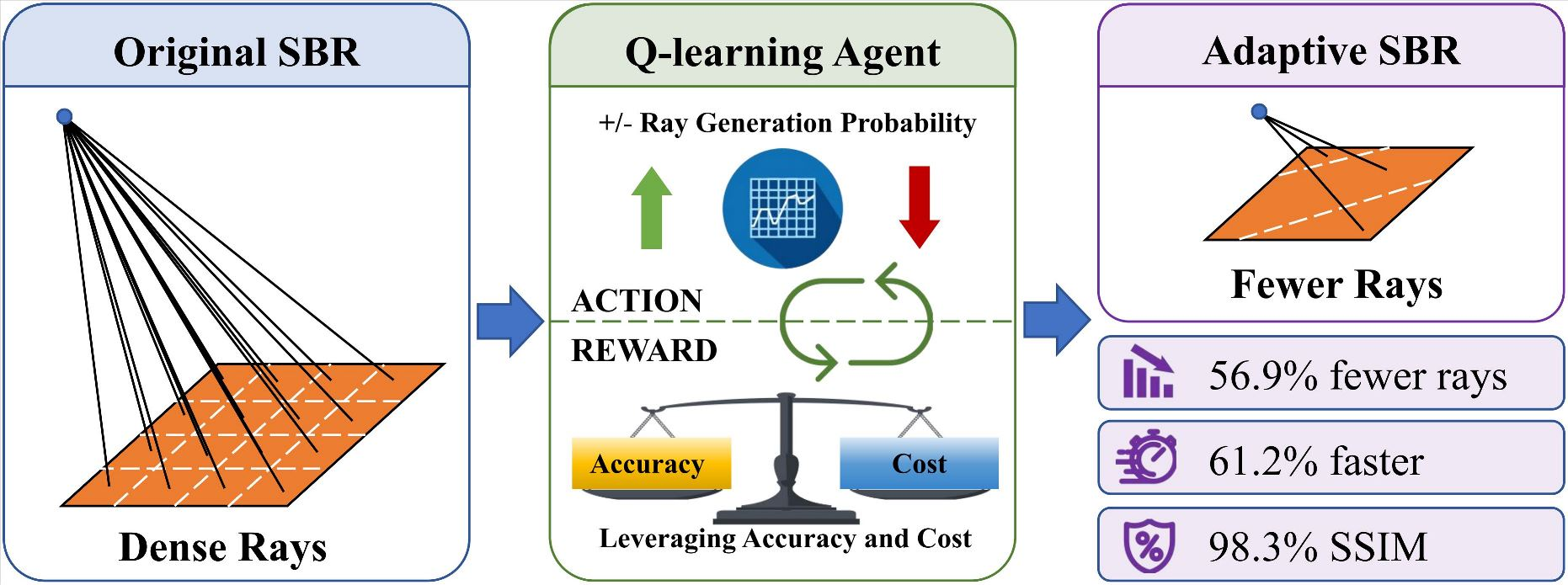
• The proposed framework accelerates the ray-tracing process by 61.2% while maintaining high similarity to the original SBR-based SAR imaging simulation.

What are the implications of the main findings?

• They bridge the gap between reinforcement learning and computational electromagnetics, offering a novel intelligent computing paradigm for electromagnetic scattering simulation.
• The method facilitates the rapid generation of large-scale, high-fidelity synthetic SAR datasets, which is crucial for training computer vision models for SAR images.

Abstract

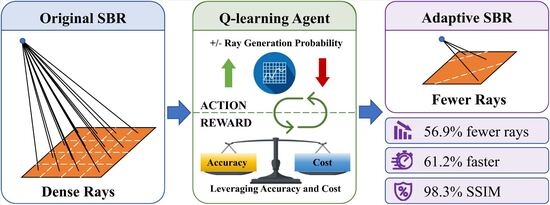
Fast synthetic aperture radar (SAR) imaging simulation is required by many computer vision applications. Although the Shooting and Bouncing Ray (SBR) method has significantly accelerated electric field calculation, the number of ray tubes is still the bottleneck for SAR image simulation speed. This paper proposes an innovative adaptive SBR method driven by Q-learning for accelerated SAR imaging simulation. The core strategy is to convert the ray tube allocation into a reinforcement learning problem. The ray-shooting plane is dynamically partitioned into localized patches, where a Q-learning agent intelligently scales the ray density in real time. By observing the geometric features of the target surface, the agent learns to employ coarser ray tubes in flat regions to eliminate redundant computation, while deploying denser ray tubes in complex areas. A multi-objective reward function is designed to balance accuracy against computational resource consumption. Numerical experiments demonstrate that the proposed Q-learning-based SBR method drastically reduces computational cost while preserving imaging similarity.

1. Introduction

Computer vision for synthetic aperture radar (SAR) images requires fast SAR imaging simulation. For example, adversarial attacks for object detection [1] models on SAR images require fast SAR imaging simulation to change the shapes of targets and spatial layouts of corner reflectors or dynamically relocating maritime vessels, and to generate a large number of candidate examples for searching. Data augmentation for SAR image object detection [2] or false target recognition [3] also requires fast SAR imaging simulation, because traditional data augmentation for optical images, such as rotations, scaling and color jittering, are physically meaningless for SAR images.

There are two main trends in accelerating SAR imaging simulation. One trend is using deep neural networks, e.g., generative adversarial networks, to generate SAR images [4]. However, these data-driven methods are not physics-based and, therefore, they cannot be used for applications that require accurate physical modeling. Another trend is using ray-tracing-based electromagnetic simulation methods, e.g., the Shooting and Bouncing Ray (SBR) method [5], to accelerate the electric field calculation in SAR imaging simulation. Although SBR-based electromagnetic calculation methods have significantly increased the speed of electric field calculation, they still need to be improved for the above-mentioned applications.

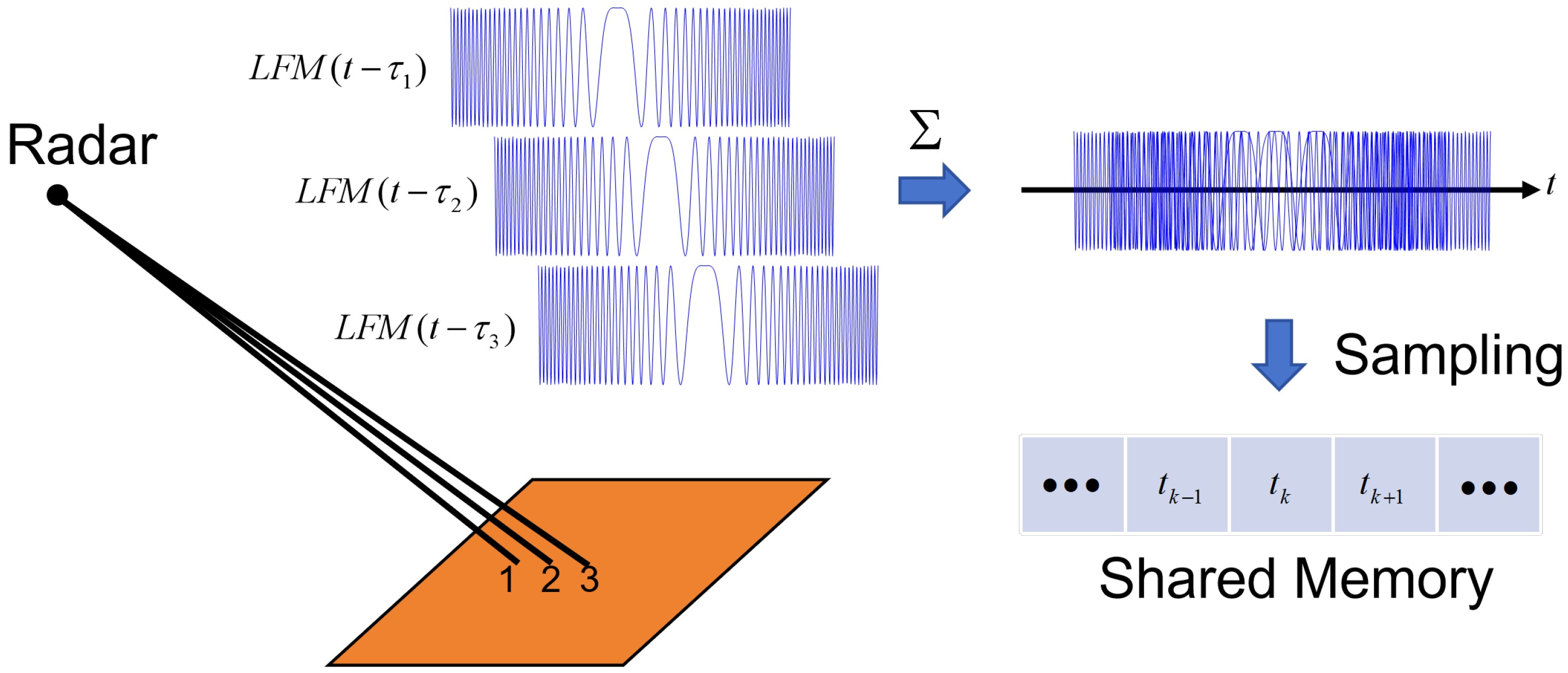
SBR-based SAR imaging simulation generally consists of two stages. Firstly, it shoots a large number of ray tubes from the radar to the target to compute the electric field from each intersection point or scattering center. Then, it aggregates the linear frequency modulation (LFM) signals from all these points to obtain the raw data for subsequent range and azimuth compression. Since SBR computations are mutually independent across different ray tubes, the ray-tracing and intersection testing phases can be efficiently accelerated by NVIDIA OptiX which utilizes RT cores for hardware-level acceleration. However, the subsequent summarization of the LFM signals from every individual scatter center or intersection point presents a severe non-parallelizable bottleneck. Aggregating a massive number of these signals is highly time-consuming (Figure 1). The motivation of the proposed method is to reduce the number of simulated rays, thereby fundamentally reducing the number of LFM signals to be aggregated.

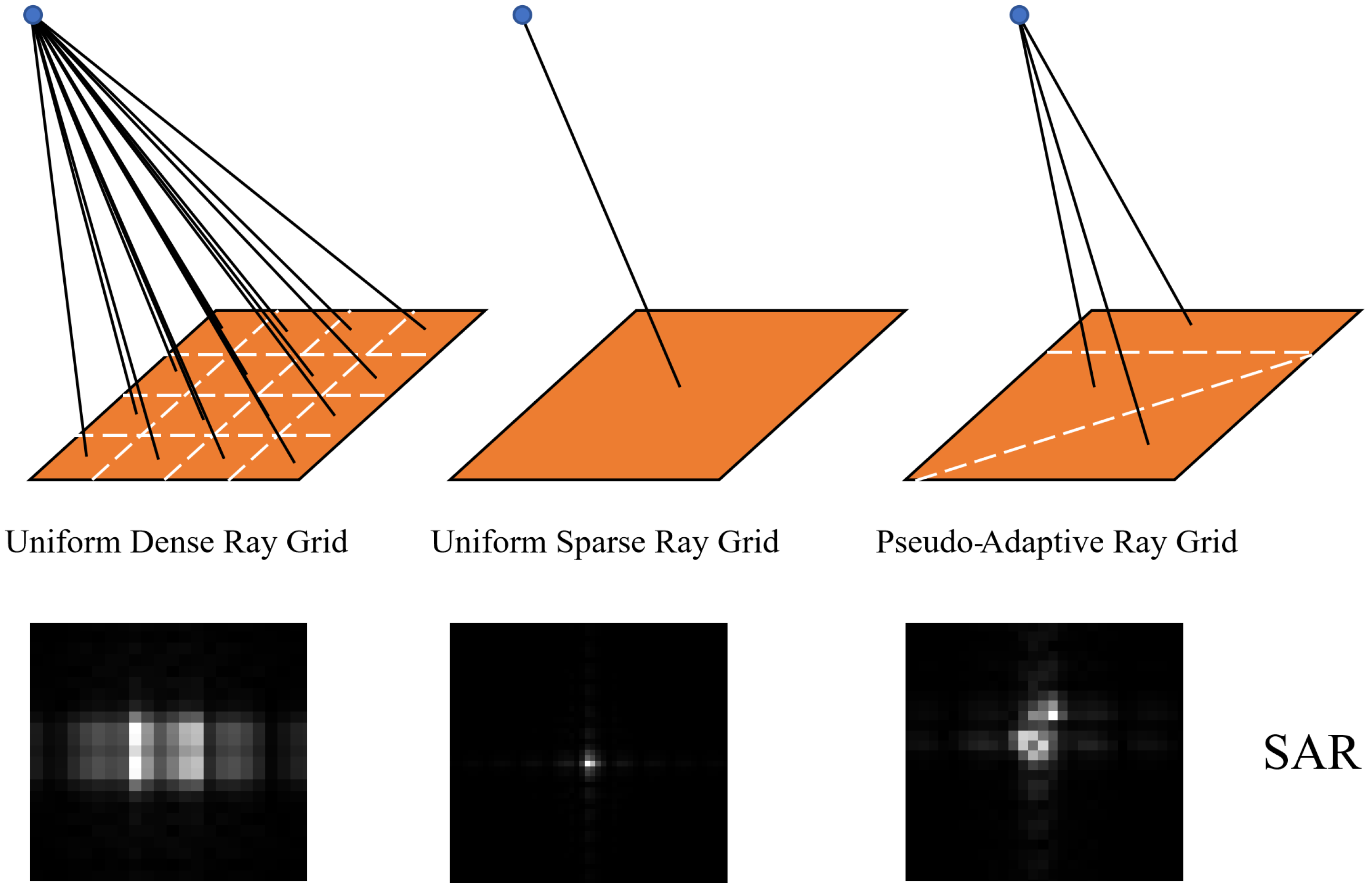
Numerous studies have proposed methods to reduce the number of rays in electromagnetic simulation for radar cross-section (RCS) calculation as well as in computer graphics for rendering. However, none of these ray reduction methods are directly suitable for SAR imaging simulation. When calculating a RCS, the far fields from all scattering centers are summarized at a single observation point. For a simple rectangular or triangle facet, we can use different ray tube layouts to calculate a RCS without losing accuracy (Figure 2). In rendering, Monte Carlo estimators are generally used to calculate the integrals in the rendering equation. The phase shifts caused by spatial propagation delays are not explicitly modeled in rendering, and therefore the ray reduction methods do not need to consider the phase preservation issue. Nevertheless, the phase issue is critical for SAR imaging, and therefore we need to design a specific ray reduction method for SBR-based SAR imaging simulation.

As shown in Figure 2, for a simple rectangular perfectly electric conducting (PEC) target, we can merge the dense grid into sparser grids or even a single ray tube to compute the RCS. However, for SAR imaging, the merging depends on the azimuth, range resolution, receiver position, etc.

To address these challenges, this paper introduces an innovative intelligent SBR framework powered by reinforcement learning to accelerate SAR imaging simulation. We formulate the ray tube scaling problem as a sequential decision-making process solved via the Q-learning algorithm. The ray-shooting plane is segmented into localized patches, each governed by a trained Q-learning agent. By analyzing a concise set of localized geometric features, the agent adaptively dictates the optimal layout of the ray tubes. It deploys coarser ray tubes in smooth, flat domains to filter out computational redundancy, while triggering fine-grained ray tube splitting in complex geometric regions to preserve phase and amplitude accuracy. Guided by a multi-objective reward function that explicitly balances echo precision against ray-tracing cost, the framework learns the optimal sampling density autonomously.

2. Related Works

Various ray reduction methods have been developed in RCS calculation and rendering. In RCS calculation, one must calculate the integrals on the intersection area between ray tubes and target facets. In rendering, one needs to estimate the integrals on each intersection point between a ray and a target facet.

Therefore, their ray reduction methods are different.

2.1. Ray Reduction in RCS Calculation

Suk et al. [6] proposed a multi-resolution grid algorithm to reduce ray counts in radar cross-section (RCS) calculation. Jin et al. [7] and Bang et al. [8] employed space-division algorithms for ray reduction. Huo et al. [9] proposed tracing individual rays and introducing virtual tubes, thereby reducing the number of traced ray tubes. Zhao et al. [10] employed a facet-neighborhood search method to reduce the number of ray–facet intersection tests. Hu et al. [11] proposed an adaptive ray tube splitting method based on whether the tube’s lateral edges intersect the target facets. They further imposed a radius threshold to prevent excessive ray tube splitting on small facets.

2.2. Ray Reduction in Rendering

Estimating the integrals in the rendering equation [12] using ray-tracing methods is a fundamental problem in computer graphics. As only a limited number of rays can be traced, the estimations suffer from high variance, which manifests as noise in the rendered images. Researchers have developed various methods to reduce the variance, including sampling, denoising, super-resolution, etc. Among them, sampling is the most relevant to our work. Sampling methods can be categorized into two types: importance sampling and adaptive sampling [13]. Importance sampling methods try to estimate a probability distribution function (PDF) that can align with the product of the measurement contribution function and the pixel reconstruction filter. Adaptive sampling methods start from a low-sample MC rendering input and then strategically allocate additional samples to enhance the image quality.

2.2.1. Importance Sampling

Importance sampling improves Monte Carlo (MC) integration by drawing samples from a proposal distribution that closely approximates the integrand, thereby reducing estimator variance for a fixed sample budget. Early neural approaches to this problem cast path guiding as a reinforcement learning (RL) task: Dahm and Keller [14] formulated direction selection as an RL problem, showing that a progressively learned policy substantially shortens average path lengths—a principle directly analogous to our goal of eliminating redundant ray tubes in flat target regions. Subsequent work introduced normalizing-flow and neural-network importance samplers that learn the full light-transport distribution and adapt online, achieving significant variance reduction compared with histogram-based guides [15,16,17,18,19,20,21,22,23]. While these methods are effective in optical rendering, they do not address the propagation-phase preservation requirement that distinguishes SAR imaging simulation from rendering (Section 3.1), and therefore cannot be applied directly to our problem.

2.2.2. Adaptive Sampling

While importance sampling redistributes the probability mass used to generate each sample, adaptive sampling addresses a complementary question: how many samples should be allocated to each spatial region? Dachsbacher [24] pioneered the use of machine learning for ray-budget decisions by classifying scene regions according to their visibility configuration and applying perception-driven level-of-detail control; co-occurrence matrices over triangle clusters provided the feature representation. The approach established that learned spatial classifiers can replace hand-crafted variance metrics without loss of image quality.

Kuznetsov et al. [25] proposed DASR, the first end-to-end convolutional adaptive sampler for MC rendering. A CNN ingests a one-sample-per-pixel noisy image together with auxiliary geometry buffers and outputs a per-pixel sampling map that redistributes an additional 3 spp budget toward high-error regions, outperforming classical variance-based heuristics across diverse scene types. Vogels et al. [26] extended this idea with an iterative two-pass scheme: after an initial fixed-rate render, an error-prediction network forecasts per-pixel error after denoising, and subsequent passes double the total sample count by concentrating new samples at predicted error peaks.

Huo et al. [27] recast the per-pixel sample-count decision as a deep RL problem, training a Deep Q-Network (DQN) on offline datasets to guide where to evaluate the incident radiance field. A companion reconstruction network then synthesizes the final four-dimensional radiance field from the adaptively acquired samples. The DQN formulation is the most direct precedent for our work: like our Q-learning agent, it observes scene features, takes discrete resource-allocation actions, and receives rewards tied to both accuracy and cost—albeit in the optical rather than the SAR domain.

Hasselgren et al. [28] extended adaptive sampling into the temporal domain, incorporating motion vectors and previous denoised frames as inputs to the sample predictor so that spatio-temporal coherence reduces both per-frame cost and flickering artefacts. Salehi et al. [29] moved away from empirical noise estimates by fitting closed-form analytic noise distributions to per-pixel rendering statistics; sampling maps are then derived from these distributions without requiring stored sample cascades, yielding faster training and higher quality at elevated sample counts. Most recently, Firmino et al. [30] showed that denoiser-output variance computed via first-order Taylor expansion and automatic differentiation is a reliable guide for iterative sample redistribution, achieving superior equal-time error across diverse scenes without training any additional networks.

3. Methodology

As the proposed method incorporates methods in signal processing (Range Doppler), electromagnetic simulation (SBR) and reinforcement learning (Q-learning), the notations may be confusing for readers from different backgrounds. For example, s is usually used to represent signal in signal processing, but it is also used to represent state in reinforcement learning. $\lambda$ is usually used to represent wavelength in electromagnetics, but it is also used to represent weight decay factor in reinforcement learning. Therefore, we divided our method into three subsections. Within each subsection, we use the notations commonly used in the corresponding field and clarify them separately. Some widely-used cross-disciplinary notations and their meanings are listed in

Table 1. Cross-disciplinary notations and confounding meanings.

Notations	Signal Processing (Section 3.1)	Electromagnetics (Section 3.2)	Reinforcement Learning (Section 3.3)
s	Transmitted/received signal	Target surface area/scattering mechanism (as subscript, e.g., $k_s$)	Environment state
$\lambda$	Operational wavelength	Operational wavelength	Weight decay factor
$\eta$	Slow-time variable/additive white noise	Intrinsic impedance of media	Learning rate
k	Discrete sampling index/chirp rate	Wavenumber in free space	Iteration index/step counter
$\mu$	Statistical mean/expectation	Magnetic permeability	Statistical mean of distribution
$\sigma$	Radar cross-section (RCS)/standard deviation	Electrical conductivity	Standard deviation of policy/noise
$ϵ$	Residual error/precision threshold	Complex permittivity	Convergence threshold
j	Imaginary unit	Imaginary unit	Imaginary unit
i	Imaginary unit	Imaginary unit/incident wave (as subscript, e.g., $E_i$)	Imaginary unit
$u,v$	—	—	Grid-cell row and column indices (Section 3.3)

.

3.1. Range Doppler Method for SAR Imaging Simulation

The Range Doppler method is a widely used algorithm for broadside SAR imaging. Suppose the radar emits a linear frequency modulation (LFM) signal, the echo signal can be expressed as

$$s\left(t\right)={\displaystyle \sum _{i=1}^N}{E}_{{\mathbf{r}}_i}\exp \left\{j2\pi \left[f_c(t-{\tau }_i)+{\displaystyle \frac{B}{2T}}{(t-{\tau }_i)}^2\right]\right\},$$

(1)

where N is the number of scattering centers, $E_{{\mathbf{r}}_i}$ is the electric field received from the i-th scattering center, ${\mathbf{r}}_i$ is the vector from the i-th scattering center to the receiver, $f_c$ is the carrier frequency, B is the bandwidth, T is the pulse duration, and ${\tau }_i$ is the time delay corresponding to the two-way travel time from the radar to the i-th scattering center. The Range Doppler method applies azimuth and range matching filters in the slow-time and fast-time domains, respectively, to obtain a SAR image. Each time the radar emits an LFM pulse, the range filter is applied to the echo signal to obtain the range profile. The range filter is given by

$$h_r\left(t\right)=\exp \left\{-j2\pi \left[f_{c}t+{\displaystyle \frac{B}{2T}}{t}^2\right]\right\}.$$

(2)

All echo signals received at different radar positions are processed by the range filter to obtain a range history. Then, the azimuth filter is applied to the range history to obtain the SAR image. The azimuth filter is given by

$$h_a\left(t\right)=\exp \left\{-j2\pi {\displaystyle \frac{2v^2{t}^2}{\lambda r_0}}\right\},$$

(3)

where v is the platform velocity, $\lambda$ is the wavelength, and $r_0$ is the reference slant range used in the matching filter. In real applications, we do not know the exact position of the i-th scattering center, so a reference range $r_0$ is used in the azimuth matching filter. The azimuth and range resolution are ${\Delta }_a=L/2$ and ${\Delta }_r=c/\left(2B\right)$, respectively, where L is the antenna length and c is the speed of light. To preserve the aspect ratio of targets, azimuth resolution is generally set to be equal to the range resolution, i.e., $L=c/B$.

In SAR simulation, we usually suppose a targeting imaging area, e.g., a square area at the center of an XOY plane. According to the flight trajectory, we can calculate the minimum and maximum ranges from the radar to the imaging area, i.e., $r_{min}$ and $r_{max}$. Then, we can determine the number of range bins by $N_r=(r_{max}-r_{min})/{\Delta }_r\ast f_s/B$, where $f_s$ is the sampling frequency. Each time the radar transmits an LFM signal, the sampled echo will be stored as a column of a signal matrix $\mathbf{S}$. The range matching filter is applied to each column of $\mathbf{S}$ and then the azimuth matching filter is applied to each row of the range-filtered signal matrix. Finally, we calculate the dB value of the azimuth- and range-filtered signal matrix to obtain the SAR image. The dynamic range of the SAR image is determined by the maximum and minimum values in the azimuth- and range-filtered signal matrix, which is usually set to 30 dB or 40 dB for visualization.

3.2. SBR Method for Electric Field Calculation

3.2.1. First-Order Scattering

The first illumination on the target surface is computed by closed-form TDPO integration on triangular facets. Every facet can be treated independently and electromagnetic echo calculation can be performed in parallel.

For a time-varying plane wave, the incident wave can be expressed as

$${\mathbf{E}}_i(\mathbf{r},t)={\mathbf{E}}_i\left(\mathbf{r}\right)·E_0\left(t\right),$$

(4)

where ${\mathbf{E}}_i\left(\mathbf{r}\right)$ indicates the amplitude and direction of the incident electric field at position $\mathbf{r}$. $E_0\left(t\right)$ indicates the waveform in time domain. As SAR imaging simulation is performed in the far-field region, the incident wave can be approximated as a plane wave. The far-field expression of TDPO integral for electromagnetic scattering from a PEC surface illuminated by a time-varying plane wave is given as

$${\mathbf{E}}_s({\mathbf{r}}_i,t)={\displaystyle \frac{1}{2\pi r_{i}c}}{\widehat{\mathbf{k}}}_s\times {\widehat{\mathbf{k}}}_s\times [{\widehat{\mathbf{n}}}^{\prime }\times ({\widehat{\mathbf{k}}}_i\times {\widehat{\mathbf{e}}}_i)]{\int }_{S_i}{\displaystyle \frac{\partial }{\partial t^{\prime }}}{E}_i\left(t^{\prime }\right)ds$$

(5)

where $r_i$ is the distance from the scattering center to the receiver, ${\widehat{\mathbf{k}}}_s$ and ${\widehat{\mathbf{k}}}_i$ are the unit propagation vectors of the scattered and incident waves, respectively, ${\widehat{\mathbf{e}}}_i$ is the polarization vector of the incident wave, and ${\widehat{\mathbf{n}}}^{\prime }$ is the unit normal vector of the scattering surface. $E_i\left(t^{\prime }\right)$ represents the incident electric field waveform at the delayed time $t^{\prime }$, defined as $t^{\prime }=t-{\tau }_i-r_i/c-({\widehat{\mathbf{k}}}_i-{\widehat{\mathbf{k}}}_s)·{\mathbf{r}}^{\prime }/c$, where ${\tau }_i$ is the reference time delay for the i-th scattering center, ${\mathbf{r}}^{\prime }$ is the position vector from the scattering center to the surface element, and $S_i$ is the effective illumination area of the i-th scattering center.

Accordingly, the surface integral $I\left(t\right)={\int }_{S_i}{\displaystyle \frac{\partial }{\partial t^{\prime }}}{E}_i\left(t^{\prime }\right)ds$ can be expressed as

$$I\left(t\right)={\displaystyle \frac{c}{{\alpha }^2}}{E}_0\left(t\right)\ast {\displaystyle \sum _{m=1}^{N_{edge}}}{I}_m\left(t\right),$$

(6)

where $E_0\left(t\right)$ is the waveform in time domain and $I_m\left(t\right)$ indicates the contribution of the m-th edge of $S_i$. $I_m\left(t\right)$ can be expressed as

$$I_m\left(t\right)={\alpha }^{\ast }·\Delta {\mathbf{e}}_m{\displaystyle \frac{c}{({\widehat{\mathbf{k}}}_i-{\widehat{\mathbf{k}}}_s)·\Delta {\mathbf{e}}_m}}\left[ϵ(t-t_m^{\prime })-ϵ(t-t_{m+1}^{\prime })\right],$$

(7)

in which $\mathit{\alpha }$ is the projection of ${\widehat{\mathbf{k}}}_i-{\widehat{\mathbf{k}}}_s$ on surface $S_i$, ${\mathit{\alpha }}^{\ast }$ is obtained by rotating $\mathit{\alpha }$ by 90 degrees clockwise on $S_i$, $\Delta {\mathbf{e}}_m$ is the vector of the m-th edge, and $ϵ$ is the Heaviside step function. Equation (7) only works when $\alpha \ne 0$. When $\alpha =0$, $I\left(t\right)$ can be expressed as

$$I\left(t\right)=\Delta S{\displaystyle \frac{\partial }{\partial t}}{E}_0(t-{\tau }_i-r_i/c-({\widehat{\mathbf{k}}}_i-{\widehat{\mathbf{k}}}_s)·{\mathbf{r}}_{{\mathbf{o}}^{\prime }}/c),$$

(8)

where ${\mathbf{r}}_{{\mathbf{o}}^{\prime }}$ is the position vector from the scattering center to the center of $S_i$, and $\Delta S$ is the area of $S_i$.

3.2.2. Multiple-Bounce Scattering

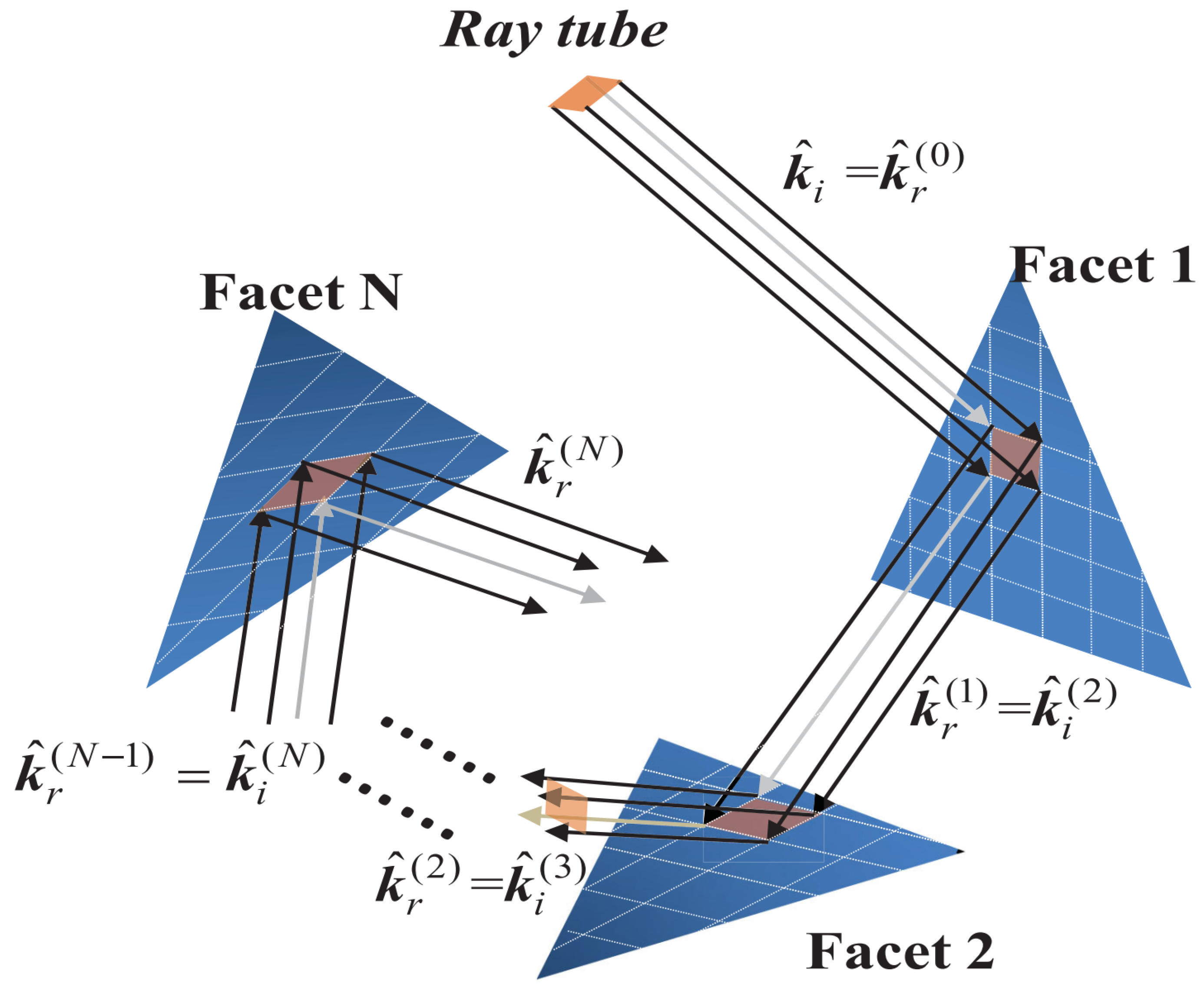
In SBR, each ray is traced through multiple bounces obeying Snell’s law as shown in Figure 3.

The N-th bounce of the incident electric field can be expressed as

$${\mathbf{E}}_i^{\left(N\right)}({\mathbf{r}}_i,t)={\mathbf{E}}_i^{\left(N\right)}\left(\mathbf{r}\right)·E_0\left(t\right).$$

(9)

The wave direction of the N-th-order incident ray is ${\widehat{\mathbf{k}}}_i^{\left(N\right)}$. According to the Snell’s reflection law, the direction of the N-th-order reflected ray is

$${\widehat{\mathbf{k}}}_r^{\left(N\right)}={\widehat{\mathbf{k}}}_i^{\left(N\right)}-2({\widehat{\mathbf{k}}}_i^{\left(N\right)}·\widehat{\mathbf{n}})\widehat{\mathbf{n}}.$$

(10)

The N-th-order reflection direction is the (N+1)-th-order incident direction; that is, ${\widehat{\mathbf{k}}}_i^{(N+1)}={\widehat{\mathbf{k}}}_r^{\left(N\right)}$. $E_i^{\left(N\right)}\left(\mathbf{r}\right)$ can be locally decomposed into its horizontal and vertical polarization components, i.e.,

$${\mathbf{E}}_i^{\left(N\right)}\left(\mathbf{r}\right)=E_{i,h}^{\left(N\right)}{\widehat{\mathbf{h}}}_i^{\left(N\right)}+E_{i,v}^{\left(N\right)}{\widehat{\mathbf{v}}}_i^{\left(N\right)},$$

(11)

where ${\widehat{\mathbf{h}}}_i^{\left(N\right)}$ and ${\widehat{\mathbf{v}}}_i^{\left(N\right)}$ are the unit vectors of the horizontal and vertical polarization components, respectively. They can be expressed as

$$\left\{\begin{array}{cc}\hfill {\widehat{\mathbf{h}}}_i^{\left(N\right)}& ={\displaystyle \frac{{\widehat{\mathbf{k}}}_i^{\left(N\right)}\times \widehat{\mathbf{n}}}{\parallel {\widehat{\mathbf{k}}}_i^{\left(N\right)}\times \widehat{\mathbf{n}}\parallel }}\hfill \\ \hfill {\widehat{\mathbf{v}}}_i^{\left(N\right)}& ={\widehat{\mathbf{h}}}_i^{\left(N\right)}\times {\widehat{\mathbf{k}}}_i^{\left(N\right)}\hfill \end{array}\right.$$

(12)

The polarization vectors of the reflected ray are given by

$$\left\{\begin{array}{cc}\hfill {\widehat{\mathbf{h}}}_r^{\left(N\right)}& ={\widehat{\mathbf{h}}}_i^{\left(N\right)}\hfill \\ \hfill {\widehat{\mathbf{v}}}_r^{\left(N\right)}& =-{\widehat{\mathbf{h}}}_r^{\left(N\right)}\times {\widehat{\mathbf{k}}}_r^{\left(N\right)}\hfill \end{array}\right.$$

(13)

The reflected electric field of the N-th bounce can be expressed as

$${\mathbf{E}}_r^{\left(N\right)}\left(\mathbf{r}\right)=E_{i,h}^{\left(N\right)}{R}_{hh}{\widehat{\mathbf{h}}}_r^{\left(N\right)}+E_{i,v}^{\left(N\right)}{R}_{vv}{\widehat{\mathbf{v}}}_r^{\left(N\right)},$$

(14)

in which $R_{hh}$ and $R_{vv}$ are the Fresnel reflection coefficients for the horizontal and vertical polarization components, respectively. For PEC targets, $R_{hh}=-1$ and $R_{vv}=1$.

For the first bounce, ${\widehat{\mathbf{k}}}_i^{\left(1\right)}={\widehat{\mathbf{k}}}_i$ and ${\mathbf{E}}_i^{\left(1\right)}\left(\mathbf{r}\right)={\mathbf{E}}_i\left(\mathbf{r}\right)$. For the (N+1)-th bounce, ${\widehat{\mathbf{k}}}_i^{(N+1)}={\widehat{\mathbf{k}}}_r^{\left(N\right)}$ and ${\mathbf{E}}_i^{(N+1)}\left(\mathbf{r}\right)={\mathbf{E}}_r^{\left(N\right)}\left(\mathbf{r}\right)$. With a process analogous to Equations (9) and (10), the (N+1)-th bounce of a scattered electric field can be calculated.

Sequentially, the scattering induced by the N-th bounce can be calculated by the TDPO integral which is similar to Equation (5). The difference is that the incident electric field should be substituted with ${\mathbf{E}}_i^{\left(N\right)}$.

It should be noticed that the waveform in time domain $E_0\left(t\right)$ will delay with multiple bounces. The time delay of the time domain can be deduced by the ray path length. Let $L^{\left(N\right)}$ be the ray path length between the N-th and (N-1)-th bounces. The time delay of the N-th bounce can be expressed as ${\tau }^{\left(N\right)}=L^{\left(N\right)}/c$.

In our paper, TDSBR is used to obtain the electric field information (including field amplitude, polarization, incident direction and so on), the intersection area information (including the position of the hit points) and the path length when a ray tube hits a target. All the information is needed by the TDPO integral equation to obtain the scattering field which is induced by the illumination of this ray tube. This shows the combination of TDSBR and TDPO. The most complex part of the combination is the calculation of the intersect area. Since the ray tube may hit more than one facet during a bounce, the divergence problem should be treated carefully.

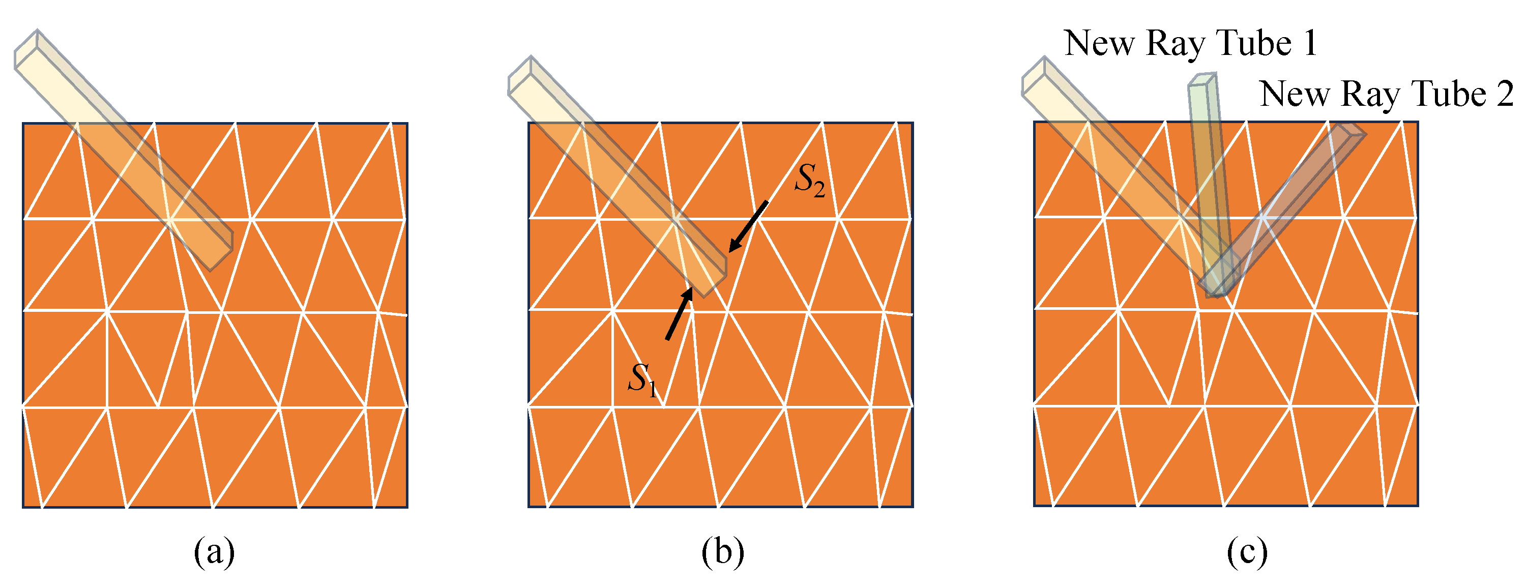
It should be noted that when one ray tube encounters the target, there are two inter-section cases: (1) The ray tube intersects with only one facet (Figure 4a). In this case, the intersection area is a quadrangle. The intersection points are easy to obtain. With the positions of the four vertexes of the quadrangle, the scattering of this area can be evaluated through TDPO. (2) The ray tube hits the facets’ boundaries and intersects with more than one facet (Figure 4b). In this case, the ray tube will split according to the shape of the facets of the target and generate new rays with different origins and reflection directions. There are two ways to solve the divergence problem. The first one is discarding the ray tube. This applies to very-small-size ray tubes and targets whose surface curvature is small. Another way is to use the adaptive partition algorithm in ray tracing. The ray tubes emitted from the ray aperture are relatively large. When the initial beam encounters the target, it splits according to the target’s shape. Each split will generate new ray tubes. The shape of the new ray tubes will change. Each new ray should be retraced. This method will increase the complexity of the problem.

Considering the ray tube size is relatively small, e.g., 1/10 of the wavelength, it is unnecessary to consider all the divergence cases. We evaluate the intersection area of the ray tube and each facet. If a ray tube hits n facets, we denote the intersection area of the ray tube and the i-th facet as $A_i$. Then, the ratio $A_i/{\sum }_{j=1}^n{A}_j$ is computed. If the ratio is larger than 40%, a new ray is generated and retraced, and the scattering is calculated. If the ratio is between 20% and 40%, the scattering from this area is calculated but a new ray tube is not generated. If the ratio is smaller than 20%, the scattering is ignored and the new ray tube is not generated. These thresholds are not newly introduced heuristics but are inherited from and validated in our prior TDSBR implementation [31], where they were established through systematic evaluation on electrically large targets.

We used NVIDIA OptiX to perform ray tracing and electric field calculation within each ray tube. More details about the implementation can be found in our previous work [31].

3.3. Q-Learning for Adaptive Ray Tube Scaling

3.3.1. Problem Formulation

The basic scheme of Q-learning is designing a Markov Decision Process (MDP) which consists of a state space S, an action space A, and a reward function R. The agent observes the state $s\in S$ of the environment and takes an action $a\in A$ according to a policy $\pi \left(a\right|s)$, which is a mapping from states to action probabilities. After taking the action, the agent receives a reward r and observes the next state $s^{\prime }$. The goal of the agent is to learn a policy that maximizes the expected cumulative reward over time.

In SBR-based SAR imaging, the radar emits one LFM pulse per pulse repetition interval as it moves along the flight trajectory. For each emitted pulse, an independent ray-tracing computation is launched to calculate the received echo signal from that aperture position. These per-pulse computations are fully independent of one another. Our Q-learning algorithm is applied independently within each single aperture-position computation: the Q-table is initialized fresh for each received-signal computation, and the algorithm converges within that computation before the result is used. No state, Q-values, or learned policy is carried across aperture positions.

Within one aperture-position computation the MDP elements are:

• Step: One pass of the while loop in Algorithm 1.
• State$s_{u,v}$: The quantized pair $(\mathrm{std}(\{{\widehat{E}}_{u,v}^{\left(k\right)}\}),\mathrm{std}(\{{\widehat{r}}_{u,v}^{\left(k\right)}\}))$ from rays shot to cell $(u,v)$ so far.
• Transition: Shooting additional secondary rays updates the running std estimates via Equation (21), yielding $s_{u,v}^{\prime }$; this is stochastic because ray positions are drawn uniformly at random.
• Terminal state: $\parallel Q_{\mathrm{new}}-Q_{\mathrm{old}}{\parallel }_{\infty }<ϵ$.

The discount factor $\gamma =0.9$ is appropriate for this short-horizon problem (10–20 steps to convergence): it down-weights decisions near convergence (${\gamma }^{10}\approx 0.35$, ${\gamma }^{20}\approx 0.12$) relative to early steps where policy changes have the largest effect on the ray budget.

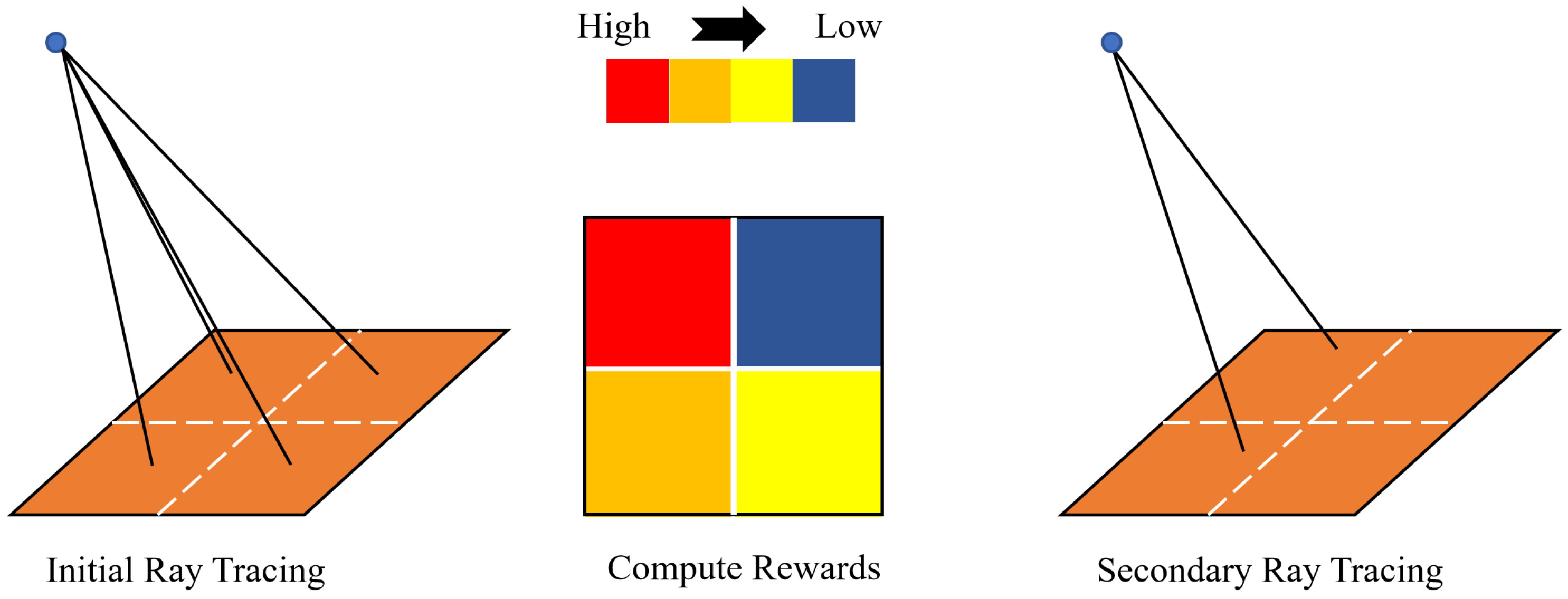
In our problem, the agent is responsible for deciding where to generate new ray tubes within one aperture-position computation. The action of the agent is to adjust the ray-shooting probability of each grid cell (Figure 5).

Algorithm 1 Q-learning-based ray generation method.

1: Initialize Q-table $Q(s,a)$ with zeros for all state–action pairs. 2: Initialize ray-shooting probability $P_{u,v}=0.9$ for all grid cells. 3: Initial ray tracing: Shoot one ray tube from the radar to the center of each grid cell. 4: while not converged do 5:       for each grid cell $(u,v)$ do 6:             Observe the current state $s_{u,v}$ 7:             Select an action $a_{u,v}$. 8:             Shoot new rays according to the updated probability $P_{u,v}$. 9:             Compute the reward $R_{u,v}$ based on the new electric fields and distances. 10:           Update the Q-table. 11:     end for 12: end while

To design the reward function, we need to consider what ensures the accuracy of the SBR-based SAR simulation. For SBR-based SAR simulation, there are two main parts that influence accuracy: (1) electric field computation; (2) signal processing. For the electric field computation part, the accuracy is mainly affected by the structure of the target. For example, if the target surface is flat, the scattering from this area will be relatively simple. However, if the target surface is complex, e.g., with many small facets or sharp edges, the scattering from this area will be more complex and multiple ray tubes will be needed to capture the scattering behavior of this area. If we were to only consider the electric field computation part, we would need to design a reward function that encourages the agent to allocate more ray tubes to the complex areas and fewer ray tubes to the flat areas. For the signal processing part, the accuracy is mainly affected by the distances from the radar to the scattering centers. If we were to only consider the signal processing part, we would need to design a reward function that encourages the agent to allocate more ray tubes to the areas that can introduce new distances. Hence, we design a combined reward function that considers both the electric field computation and signal processing parts to guide the agent.

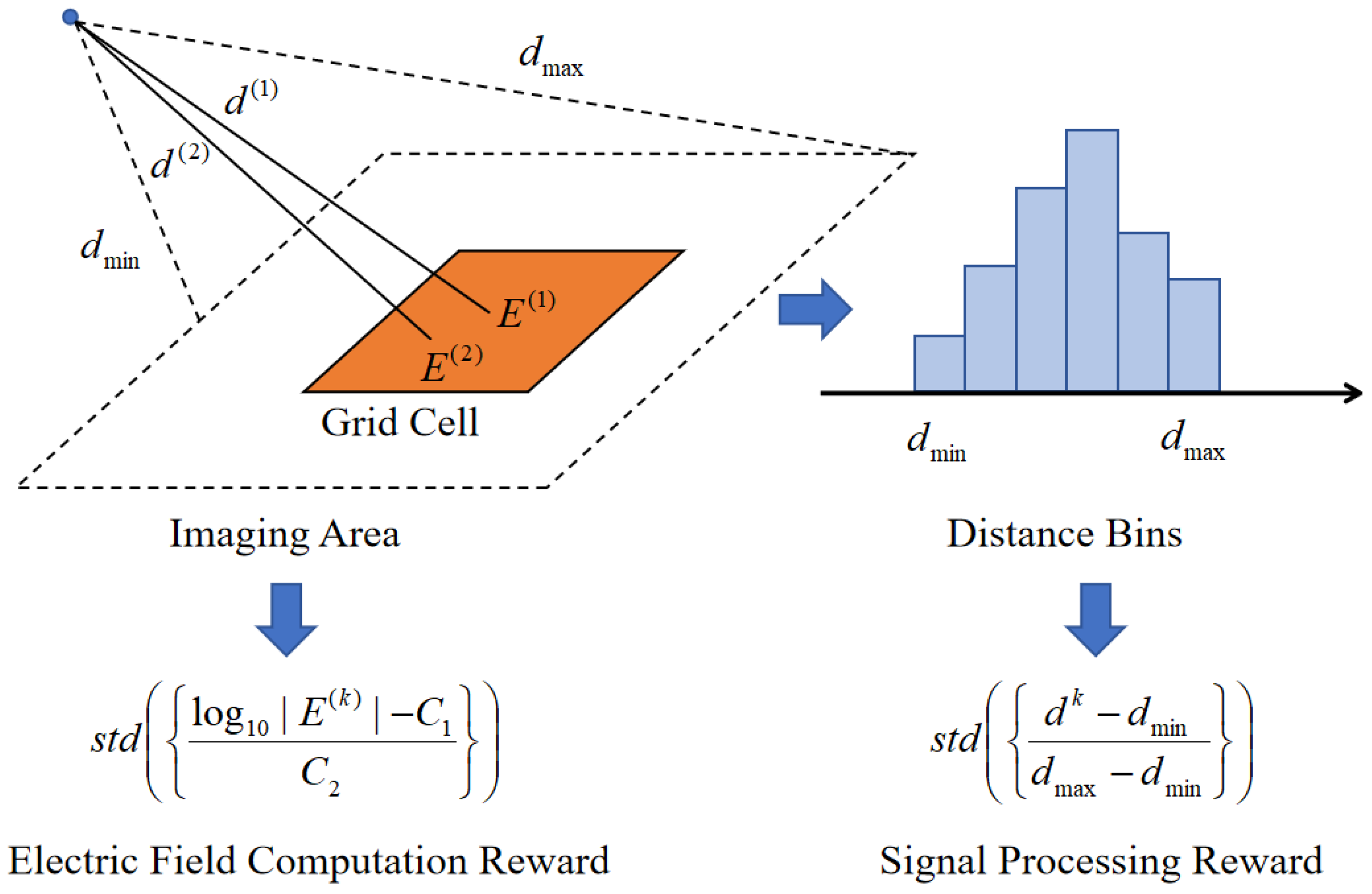
As illustrated in Figure 6, each time a ray tube is shot, the distance $d^{\left(k\right)}$ and the electric field $E^{\left(k\right)}$ are computed. We use standard deviations $std(·)$ of the normalized distances and electric fields as the rewards for the signal processing and electric field computation parts, respectively, where · represents the set of all distances or electric fields computed from the ray tubes shot in the current tracing step.

3.3.2. Constructing Reward Function

The target scene is partitioned into a matrix of discrete spatial bins (grid cells) indexed by $(u,v)$, where the size of each grid cell matches the resolution limits (${\Delta }_r\times {\Delta }_a$). Let us denote the radar position as ${\mathbf{P}}_r$. The center of the $(u,v)$-th grid cell is denoted as ${\mathbf{C}}_{u,v}=(x_i,y_j,0)$.

For each cell $(u,v)$, the initial primary ray is shot from the radar position ${\mathbf{P}}_r$ directly toward the cell center ${\mathbf{C}}_{u,v}$. The ray vector is defined as ${\mathbf{k}}_0=({\mathbf{C}}_{u,v}-{\mathbf{P}}_r)/\parallel {\mathbf{C}}_{u,v}-{\mathbf{P}}_r\parallel$. As this ray tube propagates and impinges upon the target facets contained within or behind this spatial bin, the SBR solver traces its multiple bounces and computes the final scattered electric field at the receiver via Equation (5). We denote the electric field as

$$E_{u,v}^{\left(0\right)}={\mathcal{F}}_{\mathrm{SBR}}({\mathbf{P}}_r,{\mathbf{C}}_{u,v}),$$

(15)

where ${\mathcal{F}}_{\mathrm{SBR}}$ represents the SBR method introduced in Section 3.2.

To evaluate whether the geometric features within the cell $(u,v)$ induce complex multi-path scattering or phase cancellation, a stochastic evaluation mechanism is introduced. A set of secondary points ${\mathbf{X}}_{u,v}^{\left(k\right)}$ ($k=1,2,\dots ,N$) are randomly sampled within the boundaries of the grid cell $(u,v)$ using a uniform distribution. Secondary rays are sequentially shot from ${\mathbf{P}}_r$ toward these random positions, and their corresponding scattered electric fields are denoted as

$$E_{u,v}^{\left(k\right)}={\mathcal{F}}_{\mathrm{SBR}}({\mathbf{P}}_r,{\mathbf{X}}_{u,v}^{\left(k\right)}).$$

The standard deviation of the computed electric field magnitudes within the cell is then utilized as an indicator of local scattering complexity. The standard deviation ${\sigma }_{u,v}$ is calculated as

$${\overline{E}}_{u,v}={\displaystyle \frac{1}{N+1}}{\displaystyle \sum _{k=0}^N}{E}_{u,v}^{\left(k\right)}$$

(16)

$$std\left(\left\{E_{u,v}^{\left(k\right)}\right\}\right)=\sqrt{{\displaystyle \frac{1}{N+1}}{\displaystyle \sum _{k=0}^N}{\left|E_{u,v}^{\left(k\right)}-{\overline{E}}_{u,v}\right|}^2}$$

(17)

A high value of $std\left(\left\{E_{u,v}^{\left(k\right)}\right\}\right)$ reveals that minor spatial perturbations within the resolution cell lead to drastic fluctuations in the echo amplitude or phase, signifying high geometric complexity. Conversely, a low $std\left(\left\{E_{u,v}^{\left(k\right)}\right\}\right)$ indicates a flat or homogenous surface where a single center ray is sufficient to represent the entire cell’s scattering behavior.

The magnitudes of electric fields may vary over a very large dynamic range, e.g., from ${10}^{-6}$ to ${10}^{-2}$, which makes the smaller electric fields have less effect on the computation of the standard deviation. To visualize a SAR image, a dynamic range is applied, e.g., 30 dB or 40 dB; this parameter is user-configurable and should be set consistently between $SB{R}_o$ and $SB{R}_p$ so that the normalization does not introduce a systematic bias in the comparison. That is, the electric fields should be converted to logarithmic scale and then normalized by the dynamic range. However, the maximum and minimum magnitudes of the electric fields are not known before the simulation. They depend on the target’s geometry and material properties, the radar position and so on. To solve this problem, we can use the electric fields computed from the primary rays as the reference for normalization. The normalized electric fields can be expressed as

$${\widehat{E}}_{u,v}^{\left(k\right)}={\displaystyle \frac{{\log }_{10}\left|E_{u,v}^{\left(k\right)}\right|-C_1}{C_2}},$$

(18)

where $C_1={\log }_{10}{max}_{u,v}\left|E_{u,v}^{\left(0\right)}\right|$ and $C_2=\mathrm{dynamic}\mathrm{range}\mathrm{in}\mathrm{dB}/20$. For example, a 30 dB dynamic range gives $C_2=1.5$, mapping ${\log }_{10}\left|E\right|$ to an $\mathcal{O}\left(1\right)$ interval. The denominator follows the amplitude dB convention ($20{\log }_{10}$ of an amplitude ratio), not the power convention. Then, the standard deviation can be computed based on the normalized electric fields ${\widehat{E}}_{u,v}^{\left(k\right)}$. Normalizing by the global primary-ray maximum (rather than a cell-local maximum) ensures that the reward scale remains stable across Q-learning iterations within one aperture-position computation; this is a necessary condition for consistent Q-table updates and is a deliberate design choice.

The distance bins are constructed by three parameters, i.e., the minimum range $r_{min}$, the maximum range $r_{max}$ and the range resolution ${\Delta }_r$. $r_{min}$ and $r_{max}$ can be calculated based on the radar flight trajectory and the imaging area via a constrained convex optimization problem. Without loss of generality, suppose a rectangular imaging area centered at the origin of the XOY plane. In our implementation, we segment flight trajectory according to the pulse repetition frequency (PRF) and compute the minimum and maximum distances from the radar at each position to the four edges of the rectangular area. To compute the minimum and maximum distances from a point to a line segment, we only need to compute and compare three distances: (1) two distances from the point to the two endpoints of the line segment; (2) the distance from the point to the infinite line defined by the line segment. The process can be parallelized for all radar positions.

${\Delta }_r$ is the sampling interval in the fast-time domain, which is determined by the bandwidth B of the LFM signal. According to the Nyquist sampling theorem, ${\Delta }_r$ should be less than $(r_{max}-r_{min})/2B$.

For different scenarios, the ranges of distances are different. To make the reward function more general, we can normalize the distances by the maximum range $r_{max}$, i.e., ${\widehat{d}}^{\left(k\right)}=d^{\left(k\right)}/r_{max}$. Then, the standard deviation of the normalized distances can be computed similarly to Equation (17).

The final reward function is given by

$$R_{u,v}=-\alpha ·{\widehat{n}}_{u,v}^{\left(k\right)}+{\beta }_r·std\left({\widehat{r}}_{u,v}^{\left(k\right)}\right)+{\beta }_E·std\left({\widehat{E}}_{u,v}^{\left(k\right)}\right),$$

(19)

where $\alpha$, ${\beta }_r$, and ${\beta }_E$ are three positive constants. ${\widehat{n}}_{u,v}^{\left(k\right)}$ is the normalized number of rays shot in the cell $(u,v)$, which can be expressed as ${\widehat{n}}_{u,v}^{\left(k\right)}=n_{u,v}^{\left(k\right)}/n_{\max }$, where $n_{u,v}^{\left(k\right)}$ is the number of rays shot in the cell $(u,v)$ and $n_{\max }$ is the maximum number of rays that can be calculated by the grid-cell size divided by the ray tube size. The first term in Equation (19) is the penalty for computation cost since more rays means more computations in ray tracing and signal processing. The second term is the reward for improving the signal processing accuracy since a higher standard deviation of distances indicates more new distance information is introduced by the new rays. The third term is the reward for improving the electric field computation accuracy since a higher standard deviation of electric fields indicates more complex scattering behavior is captured by the new rays.

3.3.3. Q-Learning-Based Ray Generation

The Q-learning-based ray generation method is shown in Algorithm 1.

(1) State Space (S):

The state $s_{u,v}$ of the cell $(u,v)$ is determined by quantizing its current scattering standard deviation $std\left(\left\{{\widehat{E}}_{u,v}^{\left(k\right)}\right\}\right)$ and $std\left(\left\{{\widehat{r}}_{u,v}^{\left(k\right)}\right\}\right)$ into discrete levels. As electric fields and distances are normalized, the standard deviations are in $[0,1]$. We can discretize this range into M equal intervals, resulting in a $M\times M$ state space for each cell.

(2) Action Space (A):

The action $a_{u,v}$ corresponds to adjusting the ray sampling probability $P_{u,v}$ of the cell for the next aperture simulation step:

• $a_0$ (Decrease): Reduce the sampling probability ($P_{u,v}\leftarrow max(P_{\min },P_{u,v}-\Delta P)$).
• $a_1$ (Maintain): Keep the current sampling probability unchanged.
• $a_2$ (Increase): Raise the sampling probability ($P_{u,v}\leftarrow min(P_{\max },P_{u,v}+\Delta P)$).

We set $\Delta P$ as a fixed increment, e.g., 0.05. $P_{\min }$ and $P_{\max }$ are the lower and upper bounds of the sampling probability, e.g., 0.0 and 1.0, respectively.

(3) Reward Function (R):

The reward function is given by Equation (19).

(4) Q-Table Update Rule:

The Q-values, representing the expected long-term rewards of taking specific actions under certain geometric states, are updated iteratively via the temporal difference (TD) learning rule:

$$Q(s_{u,v},a_{u,v})\leftarrow Q(s_{u,v},a_{u,v})+\eta \left[R_{u,v}+\gamma \underset{a^{\prime }}{max}Q(s_{u,v}^{\prime },a^{\prime })-Q(s_{u,v},a_{u,v})\right]$$

(20)

where $\eta$ is the learning rate and $\gamma$ is the discount factor.

Once the Q-learning converges for the current aperture position, the framework uses the converged probability map $P_{u,v}$ to determine the final ray allocation for that pulse. Cells with lower probabilities bypass the secondary random ray-tracing step, directly adopting the primary electric field as the cell’s contribution, thereby reducing the total number of simulated rays for that aperture position. This procedure is then repeated independently for each subsequent aperture position as the platform moves along the trajectory.

3.3.4. Termination Condition

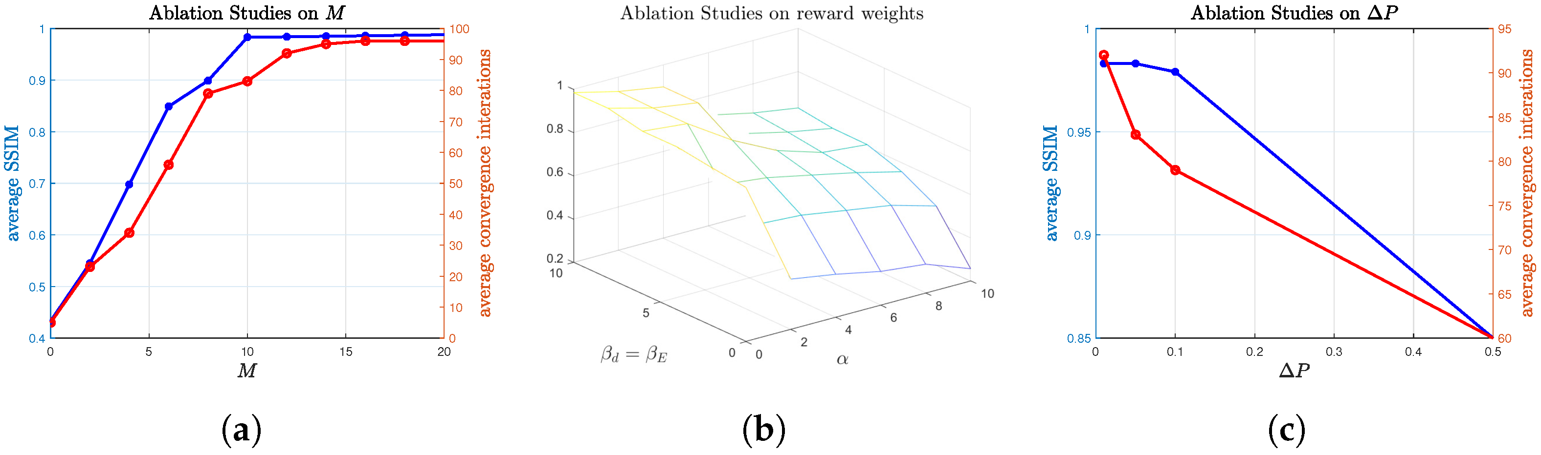
The Q-learning process uses an $\epsilon$-greedy action-selection policy (with $\epsilon =0.1$ in our experiments) to ensure that all actions are explored in every visited state, supporting empirical convergence even when formal infinite-visitation guarantees cannot be established. The process iterates until the change in Q-table values falls below a predefined threshold $ϵ$ across all state–action pairs. Since the Q-table has a finite, shared state space ($M\times M$ bins) populated by all grid cells simultaneously within one aperture-position computation, convergence is achieved within a bounded number of iterations in practice, as shown empirically in Figure 7a. For scenarios with very short apertures or very large target scenes, deep RL methods (e.g., DQN) could replace the tabular Q-learning to handle larger state spaces, which we leave as future work.

3.4. Implementation Details

We would like to emphasize three important implementation details of the proposed method.

(1) Phase issues:

To avoid redundant phase accumulation, the phase variations induced by spatial propagation delay are excluded from the high-frequency electric field calculation in the SBR phase. Since these propagation-related phase shifts are already inherently included in the LFM signal model in Equation (1), the SBR module focuses solely on capturing amplitude attenuation and the scattering/polarization phase jumps determined by the target geometry and material properties. On the other hand, one can remove the propagation phase shifts from the LFM signal model, i.e., $\exp \left(j2\pi f_c(t-{\tau }_i)\right)$ in Equation (1), and keep the SBR module unchanged.

(2) Precision issues:

Maintaining the precision of these propagation-induced phase variations is important for SAR imaging, but it poses a challenge for standard GPU hardware. The NVIDIA OptiX ray-tracing engine utilizes single-precision floating-point numbers for intersection testing. When simulating scenarios with large operational ranges, the limited precision introduces significant spatial quantization errors. These small coordinate deviations lead to severe, chaotic phase errors during LFM echo synthesis.

To mitigate this issue, we implemented a hybrid double-precision intersection refinement module. Once NVIDIA OptiX returns the primitive intersection data (i.e., the hit distance and the corresponding triangle facet index), the exact intersection coordinates are re-evaluated in double precision using the ray vector and the vertices of the hit triangle. Although performing these double-precision floating-point operations introduces a minor computational overhead, it is indispensable for eliminating phase artifacts and ensuring the fidelity of the simulated SAR images.

(3) Parallelization:

By utilizing the RT cores of NVIDIA RTX GPUs, the ray tracing is much faster than the subsequent signal processing. Compared with performing $25\times 25$ ray tracing 16 times, performing $100\times 100$ ray tracing for one launch yields a substantial overall performance improvement, because per-launch GPU kernel overhead is amortized across the larger batch. As our Q-learning-based ray generation method needs to iteratively determine whether to generate new rays within each grid cell, more iterations generally lead to greater ray number reduction. Therefore, there is a trade-off between the number of iterations and the number of rays per launch. We also need to consider the hardware limitations, such as GPU memory and the maximum number of rays that can be traced in parallel. For instance, if the targeting imaging area is $100 \mathrm{m}\times 100 \mathrm{m}$ and the carrier frequency is 3 GHz, the ray tube size will be 0.01 m, which means the total number of rays will be ${10}^8$. As we perform double-precision electric field calculations within each ray tube, a large number of rays may lead to out-of-memory issues.

(4) Iterative standard deviation computation trick:

As there may be a large number of rays within each grid cell or distance bin in every launch, computing the standard deviation of the electric fields or distances can be computationally expensive. Hence, we use a constant standard deviation for all rays in each launch. For example, if two rays are in the same distance bin, they will share the same standard deviation of distances as in the previous launch. The standard deviation of distances is updated iteratively by the Welford online algorithm [32] shown in Equation (21):

$$\left\{\begin{array}{cc}\hfill {\mu }_{new}& ={\displaystyle \frac{n_{old}}{n_{new}+n_{old}}}{\mu }_{old}+{\displaystyle \frac{1}{n_{new}+n_{old}}}\sum d_{new}\hfill \\ \hfill {\sigma }_{new}& =\sqrt{{\displaystyle \frac{n_{old}}{n_{new}+n_{old}}}{\sigma }_{old}^2+{\displaystyle \frac{1}{n_{new}+n_{old}}}\sum {(d_{new}-{\mu }_{new})}^2},\hfill \end{array}\right.$$

(21)

where ${\sigma }_{old}$ and ${\mu }_{old}$ are the standard deviation and mean of the distances of the previous $n_{old}$ rays, respectively, and $d_{new}$ is the distance of the new ray tube. That is, we do not need to access all the distances of the previous ray tubes to compute the standard deviation. The updating formula of the standard deviation of electric fields is similar to Equation (21).

4. Experiments

All our experiments were performed on a workstation equipped with an NVIDIA RTX 4090 GPU and an Intel i9-14900K. The GPU driver version was 595.79, CUDA version was 12.9 and OptiX version was 9.1.

4.1. Parameter Settings

In the LFM signal model, the carrier frequency $f_c$ was set to 12 GHz, the bandwidth B was set to 150 MHz, the antenna length L was set to 1 m, the pulse duration T was set to 1 $\mathsf{\mu }$s, the flight speed v was set to 100 m/s and the pulse repetition frequency (PRF) was set to 1 kHz.

In SBR module, we used the carrier frequency $f_c$ in SBR module to calculate the electric field for simplicity. The ray tube size was set to $1/10$ of the wavelength $\lambda$ at the carrier frequency. The tracing depth was set to 3, which means only 3 bounces were considered. Ship models are the standard benchmark class for SBR-based electromagnetic simulation, since SBR is a high-frequency asymptotic method valid for electrically large targets; this is consistent with the evaluation targets used in the SBR literature [9,10,11,31]. A tracing depth of 3 bounces is a standard and widely adopted setting for this target class, capturing the dominant first- and second-order scattering mechanisms [5,31].

In the Q-learning module, the state discrete level M was set to 10, the learning rate $\eta$ was set to 0.01, the discount factor $\gamma$ was set to 0.9, and the $\epsilon$-greedy exploration rate was set to $\epsilon =0.1$. The penalty coefficient $\alpha$ was set to 1 and the accuracy weights ${\beta }_r$ and ${\beta }_E$ were set to 10, selected via the coarse grid search shown in Figure 7b. The ray sampling probability bounds were $P_{min}=0.0$ and $P_{max}=1.0$, with step size $\Delta P=0.05$. The number of secondary evaluation rays per cell was $N=8$. The maximum ray count per cell $n_{max}$ was computed as the grid-cell area divided by the ray tube cross-sectional area ${\left(0.1\lambda \right)}^2$.

4.2. Evaluation Metrics

The proposed method aims to accelerate SBR-based SAR imaging simulation for computer vision tasks, such as data augmentation and adversarial attacks. Therefore, we used the structural similarity index measure (SSIM) [33] to evaluate the similarity between SAR images generated by the original SBR method ($SB{R}_o$) and the proposed method ($SB{R}_p$). Higher SSIM values indicate greater image similarity, and the maximum value of 1 indicates two identical images. The SSIM was applied to the processed log-magnitude (dB) SAR images produced after Range Doppler compression, which are real-valued images with a controlled dynamic range; this is consistent with established practice in SAR simulation evaluation [1,2,5]. The scope of the fidelity comparison is $SB{R}_p$ versus $SB{R}_o$: the proposed method is a ray reduction technique for SBR-based simulation, and its correctness was assessed relative to the dense-grid SBR reference, which was independently validated against measured data in [31]. Comparing against a different electromagnetic solver (e.g., MoM) would conflate the SBR approximation error with the ray reduction error, making it impossible to isolate the contribution of the proposed method.

As data augmentation and adversarial attack methods are usually used in object detection tasks, we also used the mean average precision (mAP) of a fine-tuned state-of-the-art object detection model, i.e., YOLOv12 [34], to evaluate detection performance changes. YOLOv12 is built on PyTorch 2.2.2 which relies on CUDA 12.1. Hence, there were some compatibility issues when using YOLOv12 in our CUDA 12.9 environment. To solve this issue, we used Docker to create a compatible environment for YOLOv12. We fine-tuned the YOLOv12 model on 3000 images generated by $SB{R}_o$ and tested the model on 1000 images generated by $SB{R}_o$ and $SB{R}_p$, respectively. The LFM signal parameters were kept identical, and only the radar flight path was varied when generating SAR images. A small mAP difference indicates that the proposed method can generate SAR images with performance comparable to the original method for YOLOv12.

In addition to accuracy metrics, we compared the average computation-time reduction ratio and average ray-count reduction ratio between $SB{R}_o$ and $SB{R}_p$ to evaluate efficiency gains. These reduction ratios were computed for each pair of SAR images generated by $SB{R}_o$ and $SB{R}_p$ under the same target, radar flight path, and parameter settings. Because computation time and ray count depend strongly on target geometry, flight path, and LFM parameters, their absolute values can vary substantially. Therefore, reduction ratios provide a more stable and comparable measure of efficiency improvement across different scenarios.

4.3. Results and Analysis

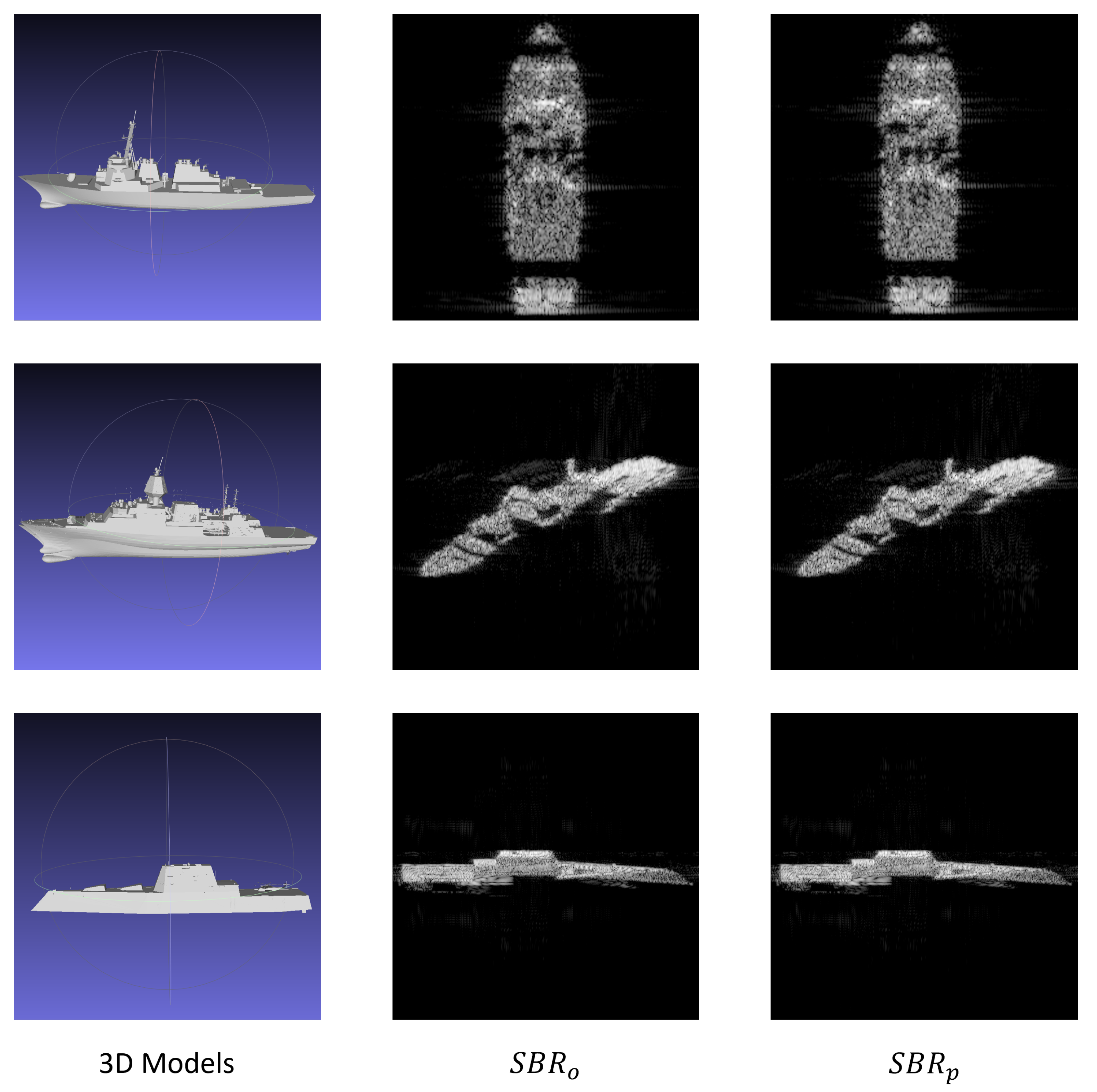
Some simulation results are shown in Figure 8. The images generated by $SB{R}_o$ exhibit higher contrast because they involve more rays and therefore yield more accurate echo calculations.

Across 7200 pairs of SAR images generated by $SB{R}_o$ and $SB{R}_p$, the average SSIM is 0.983 (minimum: 0.936; maximum: 0.995), indicating that the proposed method consistently preserves structural image similarity. Note that the images shown in Figure 8 display cropped target regions to highlight the main scattering structures; the SSIM is computed on the full images including backgrounds, which accounts for the high average value.

The mAP of YOLOv12 on SAR images generated by $SB{R}_o$ and $SB{R}_p$ is 100%, showing that $SB{R}_p$ performs comparably to $SB{R}_o$ for object-detection-oriented data augmentation and adversarial attack tasks.

The average ray-count reduction ratio is 56.9%, indicating that the proposed method reduces the number of rays by more than half. The average computation-time reduction ratio is 61.2%. The computation-time reduction ratio is higher than the ray-count reduction ratio, indicating that computational cost is not linearly proportional to the number of rays. This is mainly because GPU cores and memory bandwidth are limited, so a massive number of rays increases overall computation time in a nonlinear manner.

Table 2. Per-target results (2400 pairs per model; $SB{R}_p$ vs. $SB{R}_o$).

Target	SSIM	Ray Red. (%)	Time Red. (%)
Ship Model 1	0.980	54.8	59.3
Ship Model 2	0.984	57.1	61.4
Ship Model 3	0.987	58.9	63.0
Overall (7200 pairs)	0.983	56.9	61.2

gives per-model results.

4.4. Ablation Studies

Some hyperparameters in Q-learning have significant impacts on the performance of the proposed method. We conducted ablation studies on three groups of hyperparameters: (1) the state discrete level M; (2) the reward weights $\alpha$, ${\beta }_r$ and ${\beta }_E$; (3) the probability step size $\Delta P$. We used the SSIM as the metric to evaluate the image similarity between $SB{R}_o$ and $SB{R}_p$ under different hyperparameter settings. The results are shown in Figure 7.

As shown in Figure 7a, the image similarity increases with the state discrete level M because a higher M allows the agent to learn a more fine-grained policy for ray tube allocation. However, a higher M also increases the state space and therefore increases the convergence time of the Q-learning algorithm.

As shown in Figure 7b, the image similarity is higher when the reward weights are higher, e.g., $\alpha =1$, ${\beta }_r=10$ and ${\beta }_E=10$. When $\alpha$ is too high, the agent is more likely to reduce the ray-shooting probability, which may lead to insufficient rays and therefore lower image similarity. When ${\beta }_r$ or ${\beta }_E$ is too high, the agent is more likely to increase the ray-shooting probability, which may lead to excessive rays and therefore higher computation time. Therefore, it is important to balance the reward weights to achieve a good trade-off between image similarity and computation-time reduction.

As shown in Figure 7c, we also varied $\Delta P\in \{0.01,0.05,0.1,0.2\}$ and observed that there was no best choice of $\Delta P$. A compromise should be made between the convergence speed and the final image similarity.

5. Conclusions

In this paper, we proposed a method to accelerate SBR-based SAR imaging simulation using Q-learning. The experimental results demonstrate that the proposed method can generate SAR images with high similarity to those produced by the original SBR method while significantly reducing the computation time. This makes the method suitable for computer vision tasks such as data augmentation and adversarial attacks in SAR image analysis. The proposed method is a framework that can be extended to other ray-tracing-based electromagnetic simulation methods, SAR imaging methods (e.g., chirp scaling) and reinforcement learning algorithms.

References

1. Cui, J.; Duan, J.; Guo, W.; Peng, C.; Li, H. SAR-ESAE: Echo Signal-Guided Adversarial Example Generation Method for Synthetic Aperture Radar Target Detection. Remote Sens. 2025, 17, 3080. [Google Scholar] [CrossRef] [Scilit]
2. Tong, Y.; Xiong, K.; Liu, J.; Cao, G.; Fan, X. MAIENet: Multi-Modality Adaptive Interaction Enhancement Network for SAR Object Detection. Remote Sens. 2025, 17, 3866. [Google Scholar] [CrossRef] [Scilit]
3. Li, L.; Huang, L.; Meng, T.; Xing, C.; Yang, T.; Li, W.; Lu, P. MFE-STN: A Versatile Front-End Module for SAR Deception Jamming False Target Recognition. Remote Sens. 2025, 17, 3848. [Google Scholar] [CrossRef] [Scilit]
4. Cui, Y.; Liu, Z.; Ruan, L.; Sheng, B.; Wang, N.; Xiao, X.; Bian, X. An Azimuth-Continuously Controllable SAR Image Generation Algorithm Based on GAN. Remote Sens. 2025, 17, 3763. [Google Scholar] [CrossRef] [Scilit]
5. Li, J.; Meng, W.; Chai, S.; Guo, L.; Xi, Y.; Wen, S.; Li, K. An Accelerated Hybrid Method for Electromagnetic Scattering of a Composite Target–Ground Model and Its Spotlight SAR Image. Remote Sens. 2022, 14, 6332. [Google Scholar] [CrossRef] [Scilit]
6. Suk, S.; Seo, T.I.; Park, H.S.; Kim, H.T. Multiresolution grid algorithm in the SBR and its application to the RCS calculation. Microw. Opt. Technol. Lett. 2001, 29, 394–397. [Google Scholar] [CrossRef] [Scilit]
7. Jin, K.S.; Suh, T.I.; Suk, S.H.; Kim, B.C.; Kim, H.T. Fast Ray Tracing Using A Space-Division Algorithm for RCS Prediction. J. Electromagn. Waves Appl. 2006, 20, 119–126. [Google Scholar] [CrossRef] [Scilit]
8. Bang, J.K.; Kim, B.C.; Suk, S.H.; Jin, K.S.; Kim, H.T. Time Consumption Reduction of Ray Tracing for Rcs Prediction using Efficient Grid Division and Space Division Algorithms. J. Electromagn. Waves Appl. 2007, 21, 829–840. [Google Scholar] [CrossRef] [Scilit]
9. Huo, J.; Xu, L.; Shi, X.; Yang, Z. An Accelerated Shooting and Bouncing Ray Method Based on GPU and Virtual Ray Tube for Fast RCS Prediction. IEEE Antennas Wirel. Propag. Lett. 2021, 20, 1839–1843. [Google Scholar] [CrossRef] [Scilit]
10. Zhao, L.; Li, J.; Meng, W.; Guo, L.X.; Xi, Y.J. An Improved SBR Method Based on N-URD Emission Plane and Forward Bounding Box for Fast RCS Prediction. IEEE Antennas Wirel. Propag. Lett. 2026, 25, 746–750. [Google Scholar] [CrossRef] [Scilit]
11. Hu, S.; Guo, L.X.; Liu, Z.; Zhong, Z.; Nan, Z. A High-Performance GPU-Accelerated Ray-Tracing Method for Real-Time V2V Channel Modeling. IEEE Antennas Wirel. Propag. Lett. 2025, 24, 2527–2531. [Google Scholar] [CrossRef] [Scilit]
12. Kajiya, J.T. The rendering equation. SIGGRAPH Comput. Graph. 1986, 20, 143–150. [Google Scholar] [CrossRef] [Scilit]
13. Yan, R.; Guo, H.; Huang, L.; Xiao, N.; Li, S.; Wang, Y.; Lv, Y.; Chen, G. A Survey on Deep Learning for Monte Carlo Path Tracing. ACM Comput. Surv. 2025, 58, 1–38. [Google Scholar] [CrossRef] [Scilit]
14. Dahm, K.; Keller, A. Learning Light Transport the Reinforced Way. In Proceedings of the ACM SIGGRAPH 2017 Talks, New York, NY, USA, 30 July–3 August 2017. [Google Scholar] [CrossRef] [Scilit]
15. Zheng, Q.; Zwicker, M. Learning to Importance Sample in Primary Sample Space. Comput. Graph. Forum 2018, 38, 169–179. [Google Scholar] [CrossRef] [Scilit]
16. Bako, S.; Meyer, M.; DeRose, T.; Sen, P. Offline Deep Importance Sampling for Monte Carlo Path Tracing. Comput. Graph. Forum 2019, 38, 527–542. [Google Scholar] [CrossRef] [Scilit]
17. Müller, T.; McWilliams, B.; Rousselle, F.; Gross, M.; Novák, J. Neural Importance Sampling. ACM Trans. Graph. 2019, 38, 1–19. [Google Scholar] [CrossRef] [Scilit]
18. Müller, T.; Rousselle, F.; Keller, A.; Novák, J. Neural Control Variates. ACM Trans. Graph. 2020, 39, 1–19. [Google Scholar] [CrossRef] [Scilit]
19. Zhu, S.; Xu, Z.; Sun, T.; Kuznetsov, A.; Meyer, M.; Jensen, H.W.; Su, H.; Ramamoorthi, R. Photon-Driven Neural Reconstruction for Path Guiding. ACM Trans. Graph. 2021, 41, 1–15. [Google Scholar] [CrossRef] [Scilit]
20. Zhu, S.; Xu, Z.; Sun, T.; Kuznetsov, A.; Meyer, M.; Jensen, H.W.; Su, H.; Ramamoorthi, R. Hierarchical Neural Reconstruction for Path Guiding Using Hybrid Path and Photon Samples. ACM Trans. Graph. 2021, 40, 1–16. [Google Scholar] [CrossRef] [Scilit]
21. Dong, H.; Wang, G.; Li, S. Neural Parametric Mixtures for Path Guiding. In Proceedings of the ACM SIGGRAPH 2023 Conference Proceedings, New York, NY, USA, 6–10 August 2023. [Google Scholar]
22. Huang, J.; Iizuka, A.; Tanaka, H.; Komura, T.; Kitamura, Y. Online Neural Path Guiding with Normalized Anisotropic Spherical Gaussians. ACM Trans. Graph. 2024, 43, 1–18. [Google Scholar] [CrossRef] [Scilit]
23. Lu, H.; Chang, W.; Hedstrom, T.; Li, T.M. Real-Time Path Guiding Using Bounding Voxel Sampling. ACM Trans. Graph. 2024, 43, 1–14. [Google Scholar] [CrossRef] [Scilit]
24. Dachsbacher, C. Analyzing Visibility Configurations. IEEE Trans. Vis. Comput. Graph. 2011, 17, 475–486. [Google Scholar] [CrossRef] [Scilit] [PubMed]
25. Kuznetsov, A.; Kalantari, N.K.; Ramamoorthi, R. Deep Adaptive Sampling for Low Sample Count Rendering. Comput. Graph. Forum 2018, 37, 35–44. [Google Scholar] [CrossRef] [Scilit]
26. Vogels, T.; Rousselle, F.; McWilliams, B.; Röthlin, G.; Harvill, A.; Adler, D.; Meyer, M.; Novák, J. Denoising with Kernel Prediction and Asymmetric Loss Functions. ACM Trans. Graph. 2018, 37, 1–15. [Google Scholar] [CrossRef] [Scilit]
27. Huo, Y.; Wang, R.; Zheng, R.; Xu, H.; Bao, H.; Yoon, S.E. Adaptive Incident Radiance Field Sampling and Reconstruction Using Deep Reinforcement Learning. ACM Trans. Graph. 2020, 39, 1–17. [Google Scholar] [CrossRef] [Scilit]
28. Hasselgren, J.; Munkberg, J.; Salvi, M.; Patney, A.; Lefohn, A.E. Neural Temporal Adaptive Sampling and Denoising. Comput. Graph. Forum 2020, 39, 147–155. [Google Scholar] [CrossRef] [Scilit]
29. Salehi, F.; Manzi, M.; Roethlin, G.; Weber, R.; Schroers, C.; Papas, M. Deep Adaptive Sampling and Reconstruction Using Analytic Distributions. ACM Trans. Graph. 2022, 41, 1–16. [Google Scholar] [CrossRef] [Scilit]
30. Firmino, A.; Frisvad, J.R.; Jensen, H.W. Denoising-Aware Adaptive Sampling for Monte Carlo Ray Tracing. In Proceedings of the ACM SIGGRAPH 2023 Conference Proceedings, New York, NY, USA, 6–10 August 2023. [Google Scholar] [CrossRef] [Scilit]
31. Wei, Y.; Tian, D.; Li, J.; Wang, J.; Chai, S.; Guo, L. Efficient GPU implementation of the time-domain shooting and bouncing rays method on electrically large complex target. Waves Random Complex Media 2025, 35, 4741–4760. [Google Scholar] [CrossRef] [Scilit]
32. Welford, B.P. Note on a Method for Calculating Corrected Sums of Squares and Products. Technometrics 1962, 4, 419–420. [Google Scholar] [CrossRef]
33. Wang, Z.; Bovik, A.; Sheikh, H.; Simoncelli, E. Image quality assessment: From error visibility to structural similarity. IEEE Trans. Image Process. 2004, 13, 600–612. [Google Scholar] [CrossRef] [Scilit] [PubMed]
34. Tian, Y.; Ye, Q.; Doermann, D. YOLOv12: Attention-Centric Real-Time Object Detectors. arXiv 2025, arXiv:2502.12524. [Google Scholar]
Figure 1. Illustration of the computational bottleneck in SBR-based SAR imaging simulation. Three ray tubes are shot from the radar to the target, where each scattering center returns an LFM signal with a specific propagation delay τ i ( i = 1 , 2 , 3 ) . To obtain the raw data, all LFM signals must be aggregated at each discrete sampling time t k in the time domain; i.e., i L F M ( t i ) where t i = t k + τ i . This aggregation is strictly sequential on CPUs. On GPUs, parallel aggregation still suffers from a severe performance bottleneck due to atomic contention and memory write conflicts when processing a massive number of signals.
Remotesensing 18 02731 g001
Figure 2. Illustration of the phase preservation requirement in SBR-based SAR imaging simulation. In all three cases, the RCS can be correctly calculated based on the far-field expression of the time-domain physical optics (TDPO) integral. However, they have different SAR imaging results due to the different phase shifts of different ray tube layouts. Only the uniform dense grid layout can obtain the correct imaging result. Our proposed method learns to intelligently allocate ray tubes to preserve phase shifts while reducing ray numbers.
Remotesensing 18 02731 g002
Figure 3. Illustration of multiple bounces in SBR.
Remotesensing 18 02731 g003
Figure 4. Illustration of the ray tube intersection cases. (a) The ray tube intersects with only one facet. (b) The ray tube intersects with more than one facet. (c) The ray tube splits into new rays with new origins and directions.
Remotesensing 18 02731 g004
Figure 5. Illustration of the agent’s action. We divide the imaging area into grid cells. Each grid cell corresponds to a state in the MDP. In the initial tracing, the agent shoots one ray tube from the radar to the center of each grid cell. Then, the agent observes the state of each grid cell and takes an action to adjust the ray-shooting probability for that cell. In the secondary tracing, the agent shoots new ray tubes according to the adjusted shooting probabilities.
Remotesensing 18 02731 g005
Figure 6. Illustration of the reward computation. Each time a ray tube is shot, the distance d ( k ) and the electric field E ( k ) are computed. The standard deviations of the normalized distances and electric fields are used as the rewards for the signal processing and electric field computation parts, respectively.
Remotesensing 18 02731 g006
Figure 7. Ablation studies on (a) the state discrete level M, (b) the reward weights α , β r and β E , and (c) the probability step size Δ P .
Remotesensing 18 02731 g007
Figure 8. SAR images generated by the original SBR method ( S B R o ) and the proposed SBR method ( S B R p ).
Remotesensing 18 02731 g008