Comparison and Analysis of Four Terrestrial Water Storage Monitoring Models: A Case Study of the Loess Plateau

Highlights

What are the main findings?

• GRACE-, GLDAS-, GNSS-, and joint-inversion estimates reveal clear model-dependent differences in terrestrial water storage change over the Loess Plateau, particularly in long-term trend magnitude and seasonal behavior.
• GNSS-derived EWH shows a weaker long-term trend and stronger seasonal variability than the other estimates, suggesting that local non-elastic or non-TWS deformation processes may affect deformation-based inversion.

What are the implications of the main finding?

• GRACE- and GNSS-based TWSC estimates in geologically and anthropogenically complex regions should be interpreted with explicit consideration of soil erosion, loess collapsibility, mining disturbance, and other non-loading effects.
• The joint GNSS–GRACE inversion provides a weighted integrated estimate that improves consistency with the selected hydrological model benchmark. However, this does not prove that changes in the quality of non-TWS materials or non-elastic deformation have been ruled out.

Abstract

Accurate estimation of terrestrial water storage change (TWSC) remains challenging in regions where hydrological variability interacts with complex geological conditions and intensive human activities. Taking the Loess Plateau (LP) in the middle Yellow River region as a case study, this work integrates GLDAS simulations, GRACE observations, GNSS vertical-displacement records, a joint GNSS–GRACE inversion, and meteorological data for 2013–2024 to investigate regional TWS variability and model-dependent discrepancies. The results show that GLDAS, GRACE, GNSS, and the joint solution exhibit distinct temporal trends and spatial patterns. GRACE indicates a stronger long-term depletion signal, whereas GNSS-derived equivalent water height (EWH), which relies on the assumption of elastic surface loading, shows a weaker trend but stronger seasonal variability. This discrepancy suggests that GNSS-based inversion over the LP may be affected by non-elastic or non-loading deformation processes, such as wetting-induced loess collapse, aquifer compaction, mining-related subsidence, and other near-surface effects. In contrast, GRACE may include non-TWS mass redistribution associated with soil erosion and mineral exploitation. The joint solution is more consistent with the GLDAS-derived hydrological model benchmark than either single geodetic estimate, but this agreement should not be interpreted as direct proof of higher accuracy or complete removal of non-hydrological effects. Overall, this study highlights the need to diagnose model-dependent discrepancies, effective spatial resolution, and non-loading deformation when applying GRACE- and GNSS-based approaches to TWSC estimation in geologically and anthropogenically complex regions.

1. Introduction

Terrestrial water storage (TWS), including surface water, soil moisture, groundwater, snow water, and canopy water, is a key component of the continental hydrological cycle and plays an essential role in water resources assessment, ecological regulation, and drought monitoring [1]. Changes in TWS redistribute surface mass and induce elastic deformation of the solid Earth. Under the elastic surface-loading framework, an increase in water mass produces downward vertical displacement, whereas water loss results in elastic rebound and uplift [2]. Therefore, Global Navigation Satellite System (GNSS) vertical displacement records have been increasingly used to infer terrestrial water storage change (TWSC), usually expressed as equivalent water height (EWH), through load-deformation inversion.

However, GNSS-based EWH inversion relies on the assumption that the observed vertical displacement is mainly caused by elastic hydrological loading. This assumption may not be fully satisfied in regions where hydrological mass loading is mixed with local or near-surface deformation. GNSS stations can be affected by monument instability, poroelastic deformation, aquifer compaction, engineering-related subsidence, mining disturbance, and wetting-induced loess collapse. Some of these processes may be hydrologically triggered, but they are not necessarily equivalent to elastic surface loading. If such signals remain in the GNSS time series, the resulting EWH may contain non-elastic or non-loading components and may not represent an unbiased TWS estimate. This issue is particularly relevant to the Loess Plateau (LP), where thick collapsible loess deposits, groundwater use, mining activity, and severe soil erosion coexist.

Satellite gravimetry provides an independent observation of regional mass redistribution. The Gravity Recovery and Climate Experiment (GRACE) and GRACE Follow-On missions have been widely used to monitor large-scale TWS variations from time-variable gravity changes [3,4]. Compared with point-based GNSS observations, GRACE is less sensitive to local site deformation. Nevertheless, GRACE has coarse spatial resolution, monthly temporal sampling, leakage effects, background-model uncertainties, and data gaps between the two missions [5,6,7,8]. Moreover, GRACE responds to all detectable mass changes within its effective resolution. Therefore, non-TWS mass redistribution, such as sediment loss or mining-related mass removal, may also contribute to the observed gravity signal in regions with strong erosion and human disturbance.

Global hydrological models, such as the Global Land Data Assimilation System (GLDAS), are commonly used to support the interpretation of GRACE- and GNSS-derived estimates [9]. GLDAS provides spatially continuous simulations of land-surface water components, including soil moisture, snow water, and canopy water. However, GLDAS should not be treated as an observational truth because it contains model uncertainty and does not fully represent groundwater storage or direct anthropogenic water regulation. Agreement with GLDAS can therefore be used as a hydrological model benchmark, but not as definitive evidence that one estimate is more accurate than another.

Previous studies have shown that GNSS and GRACE can capture hydrological loading signals in many regions, and joint inversion may help exploit their complementary sensitivities [10,11,12,13,14,15,16]. However, in geologically and anthropogenically complex areas, the relationship among GNSS-derived EWH, GRACE-based TWS, and hydrological model estimates may be affected by non-elastic deformation, non-TWS mass redistribution, data resolution, and inversion assumptions. In such cases, discrepancies among datasets should not be regarded only as errors to be minimized; they can also provide useful information on method-dependent sensitivity and physical uncertainty. Therefore, quantitative evaluation of temporal correlation, seasonal behavior, long-term trend, spatial variability, and effective resolving capability is necessary before interpreting the performance of a fused solution.

The LP in north-central China provides a suitable region for examining these issues [17]. Large-scale ecological restoration has increased vegetation cover and improved environmental conditions, but it has also modified evapotranspiration, soil moisture, and regional water balance [18]. At the same time, groundwater extraction, mining activities, thick collapsible loess deposits, and sediment redistribution may influence both gravity- and deformation-based observations. These coupled natural and anthropogenic processes make the LP a representative region for assessing the reliability and limitations of multi-source TWSC monitoring.

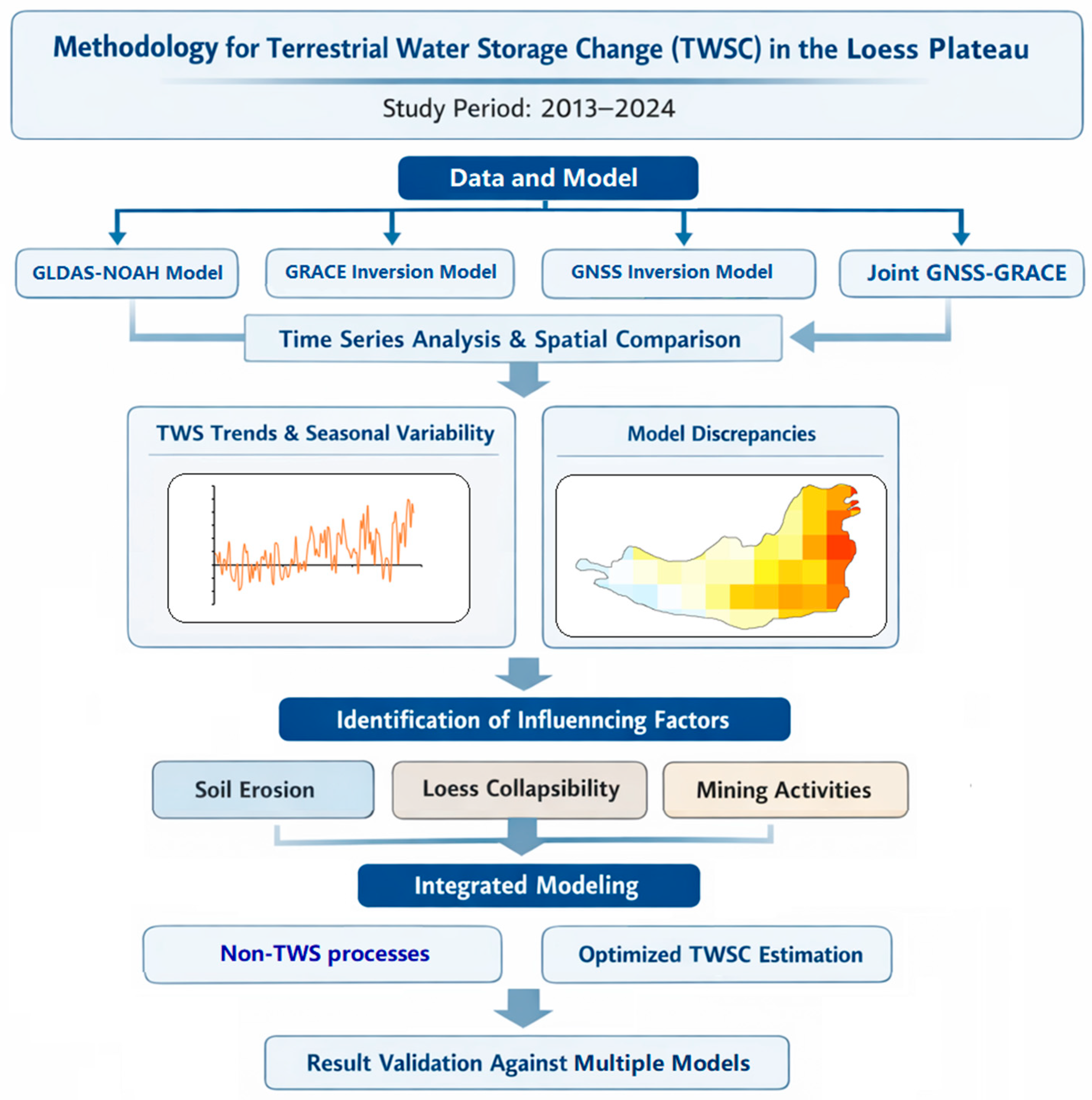
In this study, GLDAS simulations, GRACE observations, GNSS vertical displacement records from 29 stations of the Crustal Movement Observation Network of China (CMONOC), meteorological data, and a joint GNSS–GRACE inversion are integrated to investigate TWSC over the LP from 2013 to 2024. The objectives are to: (1) estimate TWS anomalies from GLDAS, GRACE, GNSS, and joint inversion; (2) quantify similarities and discrepancies among the datasets in terms of trend, seasonality, temporal correlation, and spatial pattern; (3) evaluate the joint inversion result using GLDAS as a hydrological model benchmark rather than an absolute reference; and (4) discuss the possible influence of soil erosion, loess collapsibility, mining disturbance, groundwater-related deformation, and other non-loading processes on GRACE- and GNSS-based TWSC estimates. By shifting the focus from simple model comparison to systematic discrepancy diagnosis, this study provides a more cautious and physically interpretable assessment of multi-source TWSC monitoring in complex regions. A graphic plan of the practice is indicated in Figure 1.

2. Data and Models

2.1. GLDAS Data and GLDAS-NOAH Model

Global hydrological models provide optimized, near-real-time estimates of land surface states and fluxes at relatively high spatiotemporal resolution (0.25° × 0.25°), including precipitation, evapotranspiration, and runoff [19]. These models predict key processes of the terrestrial hydrological cycle [20]. In studies of TWSC, GLDAS products are widely used as an independent reference for evaluating inversion results [21]. However, it should be noted that the TWS proxy derived from GLDAS in this paper does not directly include groundwater reserves. Therefore, consistency with GLDAS serves only as a diagnostic indicator, rather than proof of absolute accuracy.

For ease of comparison, this paper has processed the GLDAS data to a resolution of 1° × 1° and used the average values for each sector. The dataset covers the period from Jan. 2013 to Dec. 2024 and includes 144 monthly samples over the LP (33°N–41°N, 100°E–114°E). TWS anomalies were calculated by summing snow water, canopy water, and soil moisture, followed by removal of the long-term mean [22].

The climate records from the GLDAS were processed to construct temporal variations in precipitation, which were then compared with the mean monthly TWS series to examine their consistency and identify possible temporal lags. Temperature data were also organized into station-based time series to investigate the potential influence of thermal conditions on regional TWS variability.

2.2. GRACE Data and GRACE Inversion Model

Variations in TWS induce corresponding changes in Earth’s gravity field [23], which can be detected by the GRACE mission at regional to continental scales [24]. In this study, GRACE Release 06 (RL06) data provided by the Center for Space Research (CSR), were used. The dataset spans January 2003 to December 2024.

The CSR GRACE/GRACE-FO mascon product provides a regular spatial representation and is generally considered to better approximate actual surface mass variations, which facilitates regional aggregation of gridded signals using summation operators [25]. This advantage makes it suitable for constructing GRACE/GRACE-FO observation equations and for joint estimation with GNSS data. Therefore, the CSR mascon product was adopted in this study to support both independent GRACE-based estimation and joint inversion of TWS.

Within the study period, the GRACE/GRACE-FO time series contains 26 missing monthly solutions, resulting in temporal discontinuities in the observations [26]. Because joint inversion cannot be performed during these data-gap periods, a machine-learning-based reconstruction approach was adopted to fill the missing GRACE/GRACE-FO records and to produce a temporally continuous time series for subsequent analysis [27]. We used precipitation data from the European Centre for Medium-Range Weather Forecasts (ECMWF) Fifth-Generation Global Climate and Atmospheric Reanalysis (ERA5) dataset as our training data.

2.3. GNSS Data and GNSS Inversion Model

GNSS stations are indeed capable of monitoring both horizontal and vertical deformation of the Earth’s surface, however, in this type of study, the signal response of the horizontal component is weak and easily masked by noise such as tectonic movements. Therefore, GNSS studies on changes in terrestrial water storage primarily rely on vertical time series. A decrease in TWS reduces surface mass loading and induces crustal rebound. Therefore, TWSC can be inferred from surface elevation recorded by GNSS stations. However, special attention is required in the LP, where the loose soil structure and high porosity make the near-surface layers susceptible to collapse deformation under wetting conditions. In addition, terrestrial water depletion in this region is partly associated with intensive groundwater extraction [28], which may further induce non-hydrological deformation such as aquifer compaction. Therefore, GNSS-derived results should be evaluated together with other monitoring approaches.

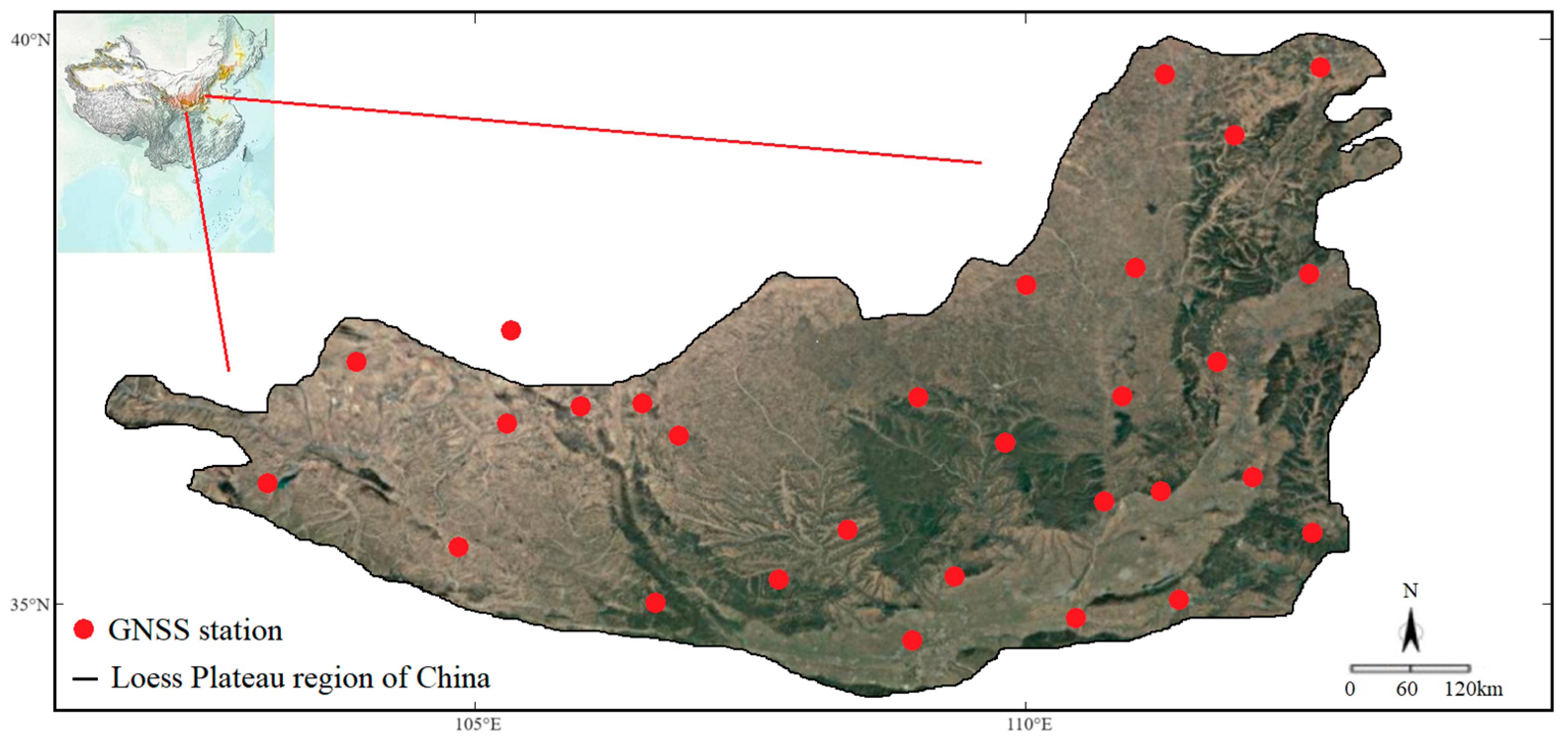
In this study, vertical displacement time series from 29 GNSS stations with relatively complete observations in the LP and its surrounding areas were selected. During the subsequent inversion process, the GNSS data must be downsampled to improve data comparability. Figure 2 shows information about the locations.

U indicates the observed vertical displacement, m is the gridded mass model over the study region, and G is the coefficient matrix constructed using the load Green’s function. Under ideal conditions, the number of observations n is equal to the number of model parameters t (n = t), and the coefficient matrix G is invertible. Then the solution defined as follows:

$$\underset{t\times l}{m}=\underset{t\times n}{G^{-1}}{U}_{t\times l}$$

(1)

Estimation of m is the main objective of the inversion. In theory, it can be solved if G is invertible. In practice, however, geophysical inversion is commonly ill-posed and underdetermined. Additional regularization constraints are therefore required.

Tikhonov regularization is typically selected, in which a regularization parameter, λ², is introduced. The resulting solution is expressed as follows:

$$m={\left(G^{T}G+{\lambda }^{2}I\right)}^{-1}{G}^{T}U$$

(2)

To improve the stability of the inversion, regularization was incorporated [29].

$${\left|\left|\underset{n\times n}{W}\left\{\underset{n\times q}{G_{g,i}}\underset{q\times l}{h_{w,i}}-\underset{n\times l}{U}\right\}\right|\right|}_2^2+{\lambda }^2{\left|\left|\underset{q\times q}{L_i}\underset{q\times l}{h_{w,i}}\right|\right|}_2^2=min$$

(3)

where W denotes the weighting matrix for GNSS vertical displacement, h_w,i is the EWH within the i-th grid cell, G_g,i represents the coefficient matrix derived from the load Green’s function, L is the Laplacian operator, λ² is the regularization parameter, n denotes the number of observed vertical displacement vector, and q is the total number of cells with the lowest resolution in the study area.

Because the convolution of the load Green’s function in the inversion is performed at the global scale, whereas the actual inversion is usually conducted for a limited regional domain, deformation induced by loads outside the study area may be treated as noise and thus contaminate the inversion results. To reduce this effect, the mass model parameters and their associated constraint matrix can be expanded to suppress the influence of external loading on mass inversion within the target region. Accordingly, Equation (3) can be rewritten as follows:

$${\left|\right|\underset{n\times n}{W}\left\{\right(\underset{n\times q}{G_{g,i}}\underset{n\times s}{G_{g,c}}\left)\right(\begin{array}{c}\underset{q\times l}{h_{w,i}}\\ \underset{s\times l}{h_{w,c}}\end{array})-\underset{n\times l}{U}\}\left|\right|}_2^2+{\lambda }^2{\left|\right|\underset{(q+s)\times (q+s)}{L_o}\left(\begin{array}{c}\underset{q\times l}{h_{w,i}}\\ \underset{s\times l}{h_{w,c}}\end{array}\right)\left|\right|}_2^2=min$$

(4)

where h_w,i and h_w,c represent the mass-loading models within the study area and outside the extended boundary, respectively; G_g,i and G_g,c denote the coefficient matrix derived from the Green’s function and the corresponding constraint matrix, respectively; n,q, and s indicate the dimensions of U, h_w,i and h_w,c respectively. This treatment helps constrain the regional mass inversion and reduce the interference from external loading signals.

The relationship between GNSS vertical displacement and TWSC can be expressed as follows:

$$d_l=G_l{X}_l+e_l$$

(5)

where d_l is the GNSS-observed vertical displacement, X_l is the TWSC inverted from GNSS measurements and expressed as EWH, e_l denotes the residual error, and G_l is the associated Green’s function matrix, defined as follows [30]:

$$G_l={\displaystyle \frac{R}{M_e}}{\displaystyle \sum _{l=0}^{\infty }{h}_l}{P}_l\left(\cos \psi \right)$$

(6)

where φ is the angular distance between the gravity-change point and the target point to be solved; M_e and R denote the mass and radius of the Earth; h_l is the load Love number for radial displacement; and P_l is the Legendre polynomial of degree l.

It should be noted that, because of differences in data characteristics and computational principles, GRACE and GLDAS are more suitable for capturing changes relative to an earlier baseline state of TWS. In contrast, GNSS-derived vertical displacement, after conversion into EWH, more effectively captures the intra-annual amplitude of TWSC.

2.4. Time Series Data Denoising Method

In time-series analyses of the four models, simple linear regression is commonly used to estimate the TWS trend. However, when the data exhibit strong seasonality and pronounced interannual variability, this approach may not adequately capture the underlying complexity of the signal.

To address this issue, singular spectrum analysis (SSA) was employed to extract meaningful components from the time series, including the long-term trend, periodic variations, and random noise [31]. SSA was used as a data-adaptive decomposition tool to visualize the dominant temporal components, while harmonic least-squares fitting was used to obtain quantitative estimates of trend, annual amplitude, semi-annual amplitude, and phase. Based on this, polynomial fitting was further applied to the TWSC to quantify the trend components of the observed variations [32]:

$$y\left(t_i\right)=p_0+p_1\left(t_i-t_0\right)+{\displaystyle {\displaystyle \sum _{k=1}^2}{A}_k\cos \left[2\pi f_k\left(t_i-t_0\right)\right]}+{\displaystyle {\displaystyle \sum _{k=1}^2}{B}_k\sin n\left[2\pi f_k\left(t_i-t_0\right)\right]}+{\epsilon }_{i}i=1,2,\dots ,m$$

(7)

where y(t_i) is the EWH variation in TWS at epoch t_i is the initial time of the series, p₀ and p₁ are the linear trend coefficients, f_k(k = 1, 2) denote the signal frequencies, A_k and B_k (k = 1, 2) represent the amplitudes of the annual and semi-annual components, respectively, and ε_i is the fitting residual.

Here, μ_l = p₀ + p₁t represents the linear trend, and μ_c = Acos(2πft + Φ) denotes the seasonal component, where Φ is the phase. To facilitate comparison among different time series, the trend was removed so that the intrinsic variability of the signals could be analyzed more clearly. A model-based detrending procedure was therefore adopted. First, a linear function was fitted to each time series, and its slope was used to represent the rate of mass change. Subsequently, a cosine function was fitted to the detrended series to characterize seasonal variability. Next, obtain the non-seasonal series:

$$y_1=y\left(t_i\right)-{\mu }_1,y_2=y_1-{\mu }_c$$

(8)

where y(t_i) is the original time series, μ₁ is the linear trend model fitted to the original series, and y₁ is the detrended time series, representing the residual fluctuations. μ_c denotes the cosine model fitted to the detrended fluctuations, and y₂ is the resulting non-seasonal time series. This treatment facilitates subsequent analysis of the relationships between TWS variability and climatic or anthropogenic factors.

For GNSS vertical deformation series, outliers exceeding three times the root mean square error were removed, along with obvious step-like offsets [33]. Such offsets may result from earthquakes or equipment replacement [34]. The secular component was retained for the TWS inversion and was evaluated later in the time-series analysis. Because surface deformation induced by TWSC over the LP is mainly expressed as an annual signal, preprocessing of the GNSS series in this study focused on removing outliers while preserving the annual component.

The GNSS time series was then modeled to reduce the effects of step signals and tectonic deformation [35]:

$$y\left(t_i\right)=y_0+v_0{t}_i+{\displaystyle \sum _{k=l}^2\left[A_k\cos \left(2k\pi t_i\right)+B_k\sin \left(2k\pi t_i\right)\right]+{\displaystyle \sum _{j=1}^n{g}_{j}H\left(t_i-T_{gj}\right)}}+e\left(t_i\right)$$

(9)

where t_i denotes time, y is the observation, y₀ is the initial position, v₀ is the linear velocity, A_k and B_k represent the seasonal amplitudes, with k = 1 and k = 2 corresponding to the annual and semi-annual signals, respectively. g_j denotes the step term, H is the Heaviside step function, T_gj is the epoch at which the step occurs, and e(t_i) represents the noise. All parameters in Equation (9) were estimated based on the least-squares criterion.

Finally, the GNSS time series was resampled to match the temporal resolution of GRACE data.

2.5. Joint GNSS–GRACE Inversion Model

Because the GRACE observations were ultimately converted to EWH, which can be expressed in vertical height change, only the GNSS vertical displacement component was converted to EWH variation for subsequent analysis. The independent GNSS inversion model can be written as follows [36]:

$$\Vert {\left(Gm-y\right)}^{-1}{\Vert }^2+{\beta }^2\Vert Lm{\Vert }^2\to \min$$

(10)

where y denotes the GNSS vertical displacement, G is the load Green’s function coefficient matrix derived from the load Love numbers, m represents the terrestrial water load expressed as EWH, L is the Laplacian smoothing operator, β is the smoothing factor, during two-dimensional gridded visualization of the data, boundary conditions must also be taken into account; accordingly, different Laplacian smoothing operators were designed for boundary cells and boundary vertices.

To integrate GNSS and GRACE/GRACE-FO data, a combined observation equation was constructed as follows:

$$SM=Sm$$

(11)

$$\left.\begin{array}{r}\hfill d={\left[\begin{array}{rr}\hfill y& \hfill SM\end{array}\right]}^T\\ \hfill A={\left[\begin{array}{rr}\hfill G& \hfill S\end{array}\right]}^T\\ \hfill W{\left({\alpha }^2\right)}^{-1}=\left[\begin{array}{cc}{\alpha }^2{\sigma }_{GNSS}^2& 0\\ 0& {\sigma }_{CSR}^2\end{array}\right]\end{array}\right\}$$

(12)

$$\Vert \left(Am-d\right){\Vert }^{2}W{\left({\alpha }^2\right)}^{-1}+{\beta }^2\Vert Lm{\Vert }^2\to \min$$

(13)

where S denotes the summation operator that aggregates gridded values within each 1° CSR mascon, M is the EWH observation from the CSR mascon product, d and A are the observation vector and coefficient matrix of the joint inversion system, respectively, W(α²)⁻¹ is the observation weighting matrix, and α is the weighting factor used to balance the relative contributions of GNSS and GRACE. The joint inversion objective function can be expressed as:

$$\widehat{m}={\left(A^{T}W{\left({\alpha }^2\right)}^{-1}A+{\widehat{\beta }}^2{L}^{2}L\right)}^{-1}{A}^{T}W{\left({\alpha }^2\right)}^{-1}d$$

(14)

The Akaike Bayesian Information Criterion (ABIC) was adopted to determine the optimal weighting and smoothing parameters [37,38]:

$$ABIC\left({\alpha }^2,{\beta }^2\right)=n\lg s\left(m\right)+\lg \Vert A^{T}W{\left({\alpha }^2\right)}^{-1}A+{\beta }^2{L}^{T}L\Vert -\lg \Vert {\beta }^2{L}^{T}L\Vert +\lg \Vert W\left({\alpha }^2\right)\Vert +C$$

(15)

$$s\left(m\right)={\left[Am-d\right]}^{T}W{\left({\alpha }^2\right)}^{-1}\left[Am-d\right]+{\beta }^2{m}^T{L}^{T}Lm$$

(16)

where n denotes the number of observations, ‖·‖ represents the product of the non-zero eigenvalues of the matrix, and C is a constant that can be omitted. The optimal regularization parameter is identified at the minimum ABIC value.

2.6. Checkerboard Test

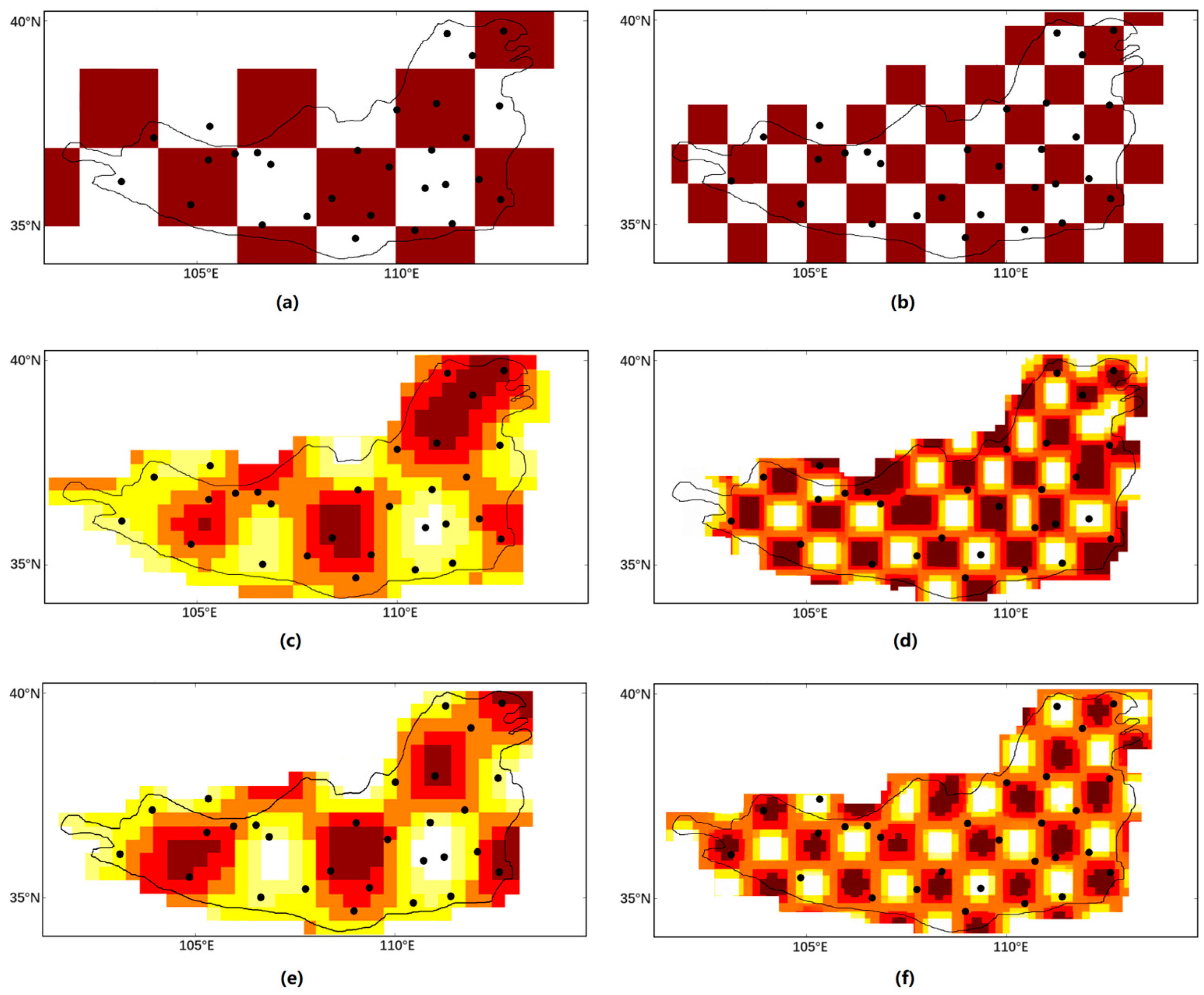
To evaluate the spatial resolution and stability of the GNSS-based mass inversion over the LP, a checkerboard (CHE) test was conducted using the actual distribution of the 29 stations in Figure 2. Following the general procedure of synthetic mass-load experiments, an artificial EWH field with alternating positive and zero anomalies was first constructed over the study area. We tested the model’s ability to recover spatial patterns, amplitude differences, and the boundaries of major anomalies. We set up controlled trials using two grid sizes: 2° × 2° and 1° × 1°, the brown and white checkerboard patterns represent input EWH signals of 300 mm and 0 mm, respectively. Figure 3 is the CHE test.

Although CHE testing is not perfect due to the distribution of sites, the current results are sufficient to support large-scale EWH pattern over the LP. The alternating positive and zero anomaly structure is broadly preserved at the regional scale, suggesting that the current station network provides useful constraints for identifying long-wavelength TWS variations. However, the recovered amplitudes are smoothed relative to the prescribed input, and the CHE boundaries become less distinct in areas with sparse station coverage, especially near the western and northern margins of the study region. This pattern indicates that the GNSS-only inversion is suitable for interpreting regional-scale TWS anomalies but has limited ability to resolve short-wavelength or highly localized mass changes. Therefore, the spatial results derived from GNSS should be interpreted together with station-density information and should not be over-interpreted in poorly constrained areas. The CHE test supports the use of the GNSS inversion for large-scale spatial comparison, while also confirming the need for GRACE constraints, hydrological model benchmarks, or additional geodetic observations to improve the robustness of fine-scale TWS estimates.

3. Results

3.1. Temporal Characteristics of TWS Variations

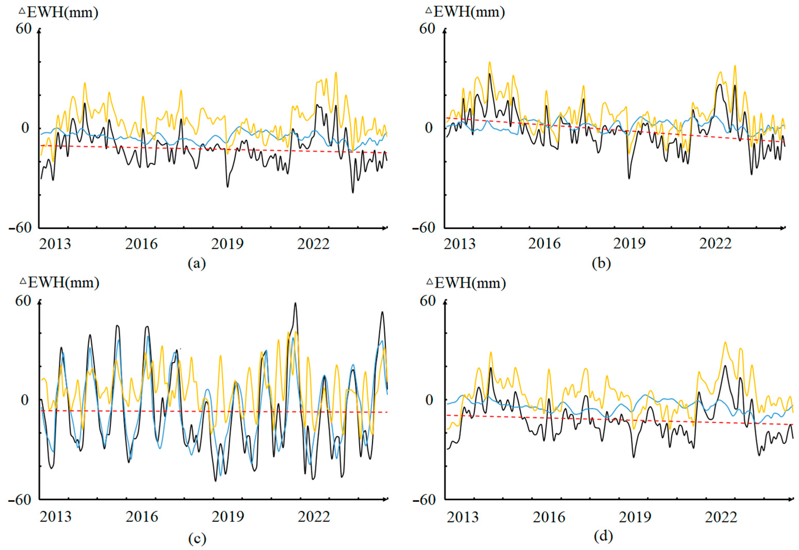
After preprocessing the four datasets, TWS time series expressed as EWH were obtained for the LP, and their temporal trends were analyzed. To further investigate temporal variability, SSA was used to decompose each model into trend, seasonal, and residual components [39]. In Figure 4, the original time series is shown by the black curve, while the trend, seasonal, and residual components are represented by red dashed, blue, and yellow curves, respectively.

The annual trends and cumulative changes derived from the four estimates are summarized in

Table 1. Linear trends of EWH derived from different models over the LP for the period 2013–2024.

Model	Trend (mm/Year)	Cumulative Change (mm, 12 Years)
GLDAS	−1.20	−14.40
GRACE	−2.77	−33.24
GNSS	−0.24	−2.88
joint GNSS-GRACE	−1.48	−17.76

.

All four estimates indicate net TWS depletion over the LP during 2013–2024, but the magnitude of the long-term trend differs substantially among datasets. Therefore, the temporal results should not be interpreted as complete consistency among GLDAS, GRACE, GNSS, and the joint solution. Instead, they reveal clear model-dependent differences in trend magnitude.

The SSA decomposition further shows that the four time series differ in both long-term trend and seasonal behavior. Compared with GLDAS, GRACE, and the joint solution, the GNSS-derived EWH series exhibits a weaker long-term decline but a more pronounced seasonal component. This feature may partly reflect the sensitivity of GNSS vertical displacement to short-term hydrological loading. However, over the LP, the GNSS signal may also include deformation processes that are not equivalent to elastic TWS loading, such as wetting-induced loess collapse, aquifer compaction, poroelastic response, mining-related subsidence, and station-scale environmental effects. Therefore, the stronger seasonal variability in the GNSS-derived EWH series should be interpreted cautiously and should not be attributed solely to hydrological storage change.

The GRACE-derived series shows a stronger long-term depletion signal than GLDAS. This difference may be related to the fact that GRACE detects regional-scale mass redistribution, including hydrological storage change as well as possible non-TWS mass changes within its effective footprint. In contrast, GLDAS represents a land-surface hydrological model estimate and does not fully account for groundwater storage or direct anthropogenic water regulation. Therefore, GLDAS is used here as a hydrological model benchmark for comparison, rather than as an absolute reference for accuracy assessment.

The joint solution shows intermediate temporal behavior between the GRACE- and GNSS-derived estimates and is closer to the GLDAS-derived benchmark in terms of long-term variation. This suggests that the joint inversion balances the stronger depletion signal detected by GRACE and the weaker trend inferred from GNSS. However, closer agreement with GLDAS should not be interpreted as direct evidence that non-TWS mass signals or non-elastic deformation effects have been completely removed.

To quantitatively evaluate the temporal consistency between the joint inversion and the individual datasets, Pearson correlation analysis was performed using monthly time series at the 29 GNSS stations. For each station, the joint solution was compared with the corresponding GNSS-derived EWH, the GRACE-derived EWH extracted from the grid containing the station, and the GLDAS-derived TWS anomaly series. The resulting correlation coefficients were grouped into three intervals, and the number of stations within each interval is summarized in

Table 2. Distribution of Pearson correlation coefficients between the joint solution and the GNSS-, GRACE-, and GLDAS-derived time series at the 29 GNSS stations.

Range of r	GNSS	GRACE	GLDAS
0.6~0.8	2	11	13
0.4~0.6	19	18	16
Less than 0.4	8	0	0

.

These results indicate that the temporal variability of the joint solution is closer to the large-scale hydrological signals represented by GRACE and GLDAS than to the GNSS-only estimates. The lower correlation with GNSS may reflect the influence of local deformation signals in the GNSS vertical displacement records, which are not fully consistent with regional elastic hydrological loading. However, the relative contribution of each dataset should be assessed through sensitivity tests analysis.

Overall, the temporal analysis indicates that the main feature of the multi-source comparison is structured disagreement rather than simple agreement. GLDAS, GRACE, GNSS, and the joint solution capture regional TWS variability from different physical perspectives. Their discrepancies provide useful evidence for identifying possible non-TWS mass redistribution, non-elastic deformation effects, and method-dependent uncertainties in TWSC estimation over the LP.

3.2. Spatial Characteristics of TWS Variations

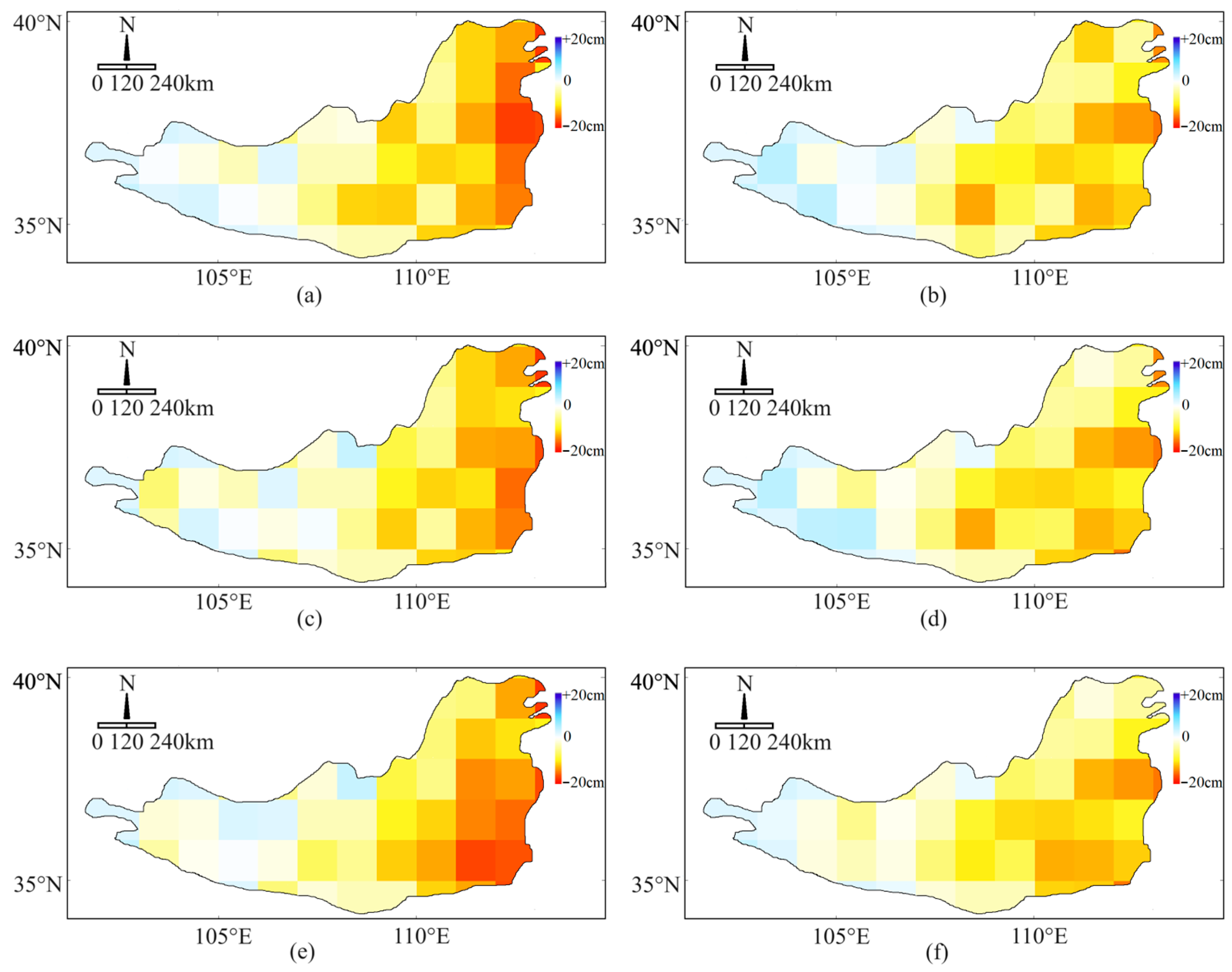
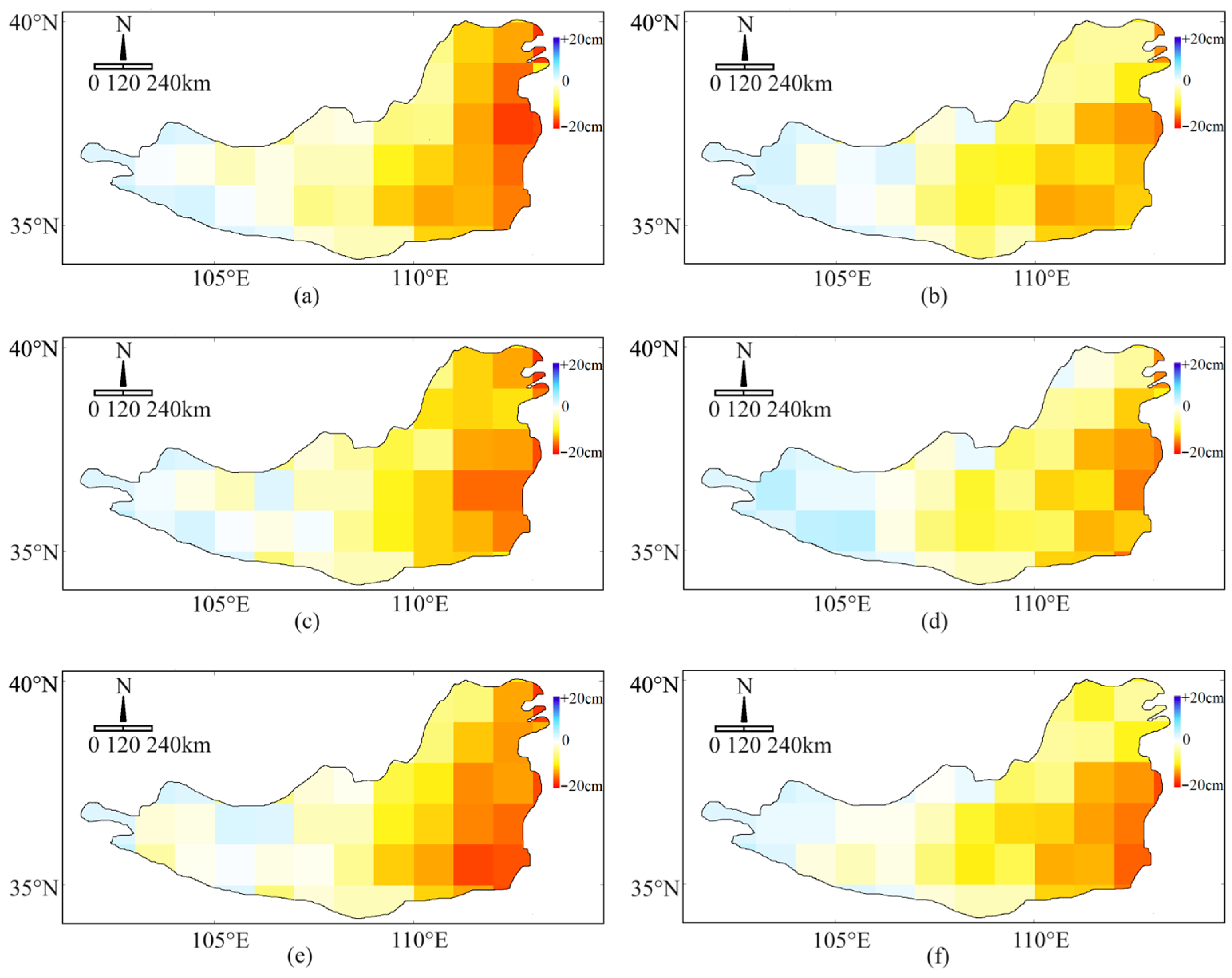
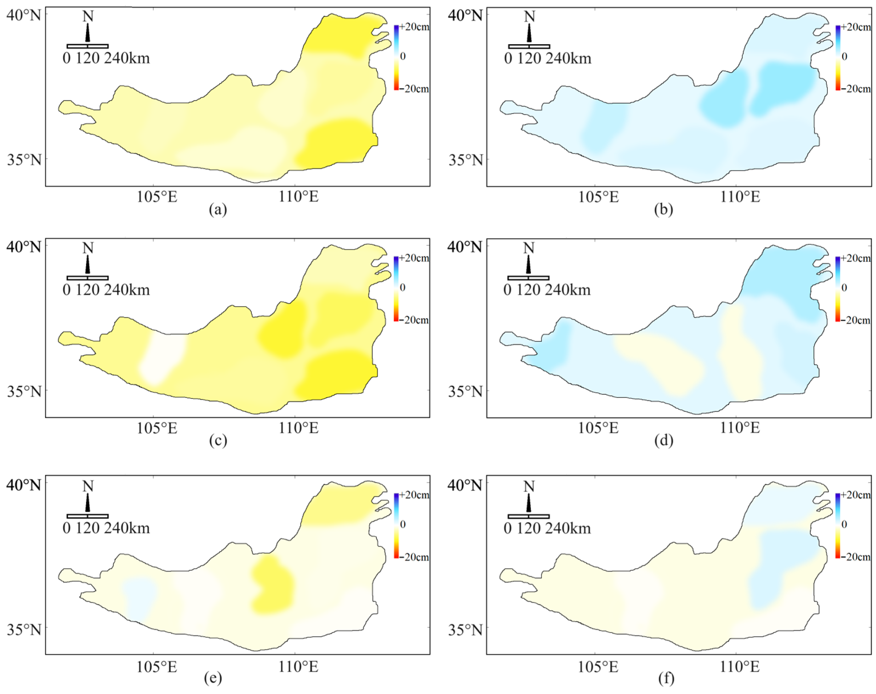
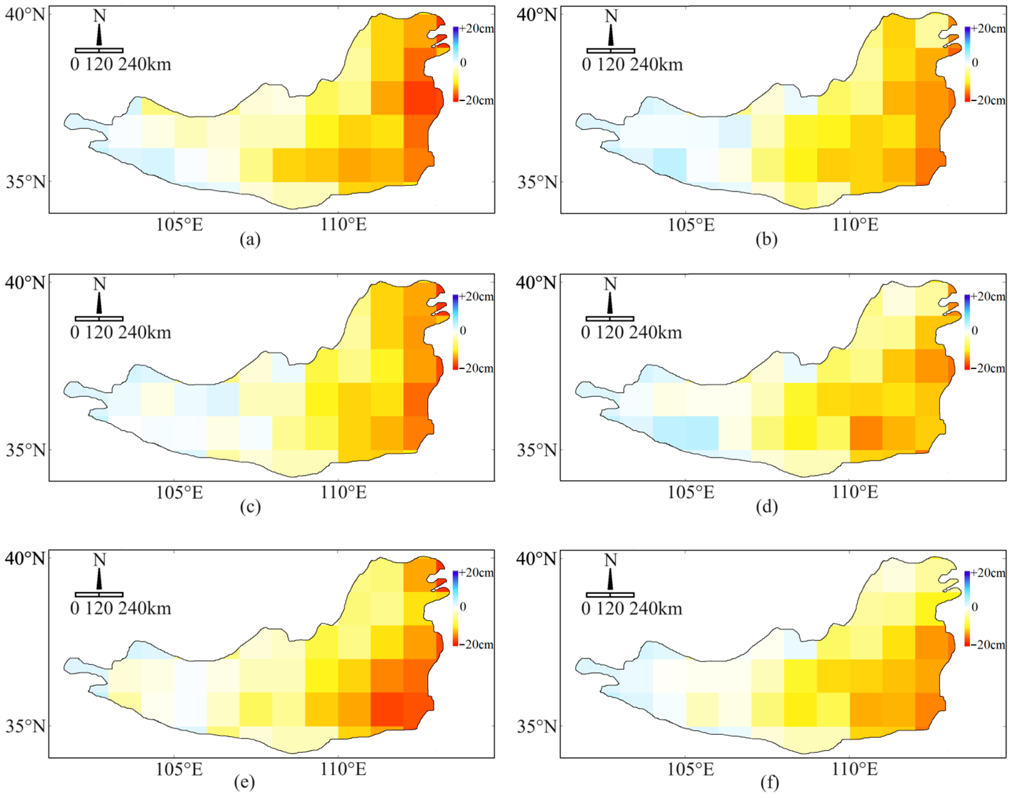
The spatial distributions shown in Figure 5, Figure 6, Figure 7 and Figure 8 represent TWS anomalies expressed as EWH relative to the reference baseline used in each dataset, rather than absolute TWS. The six selected months provide snapshots of seasonal and interannual spatial variability in January and July of 2016, 2020, and 2024.

The GLDAS, GRACE, and joint results show broadly comparable large-scale patterns, although their anomaly magnitudes and gradients differ. In the selected months, these three estimates generally indicate stronger negative TWS anomalies in parts of the eastern and northeastern LP than in the western sector, especially during winter. This spatial contrast is broadly consistent with the higher intensity of agricultural water use, groundwater abstraction, mining activity, and human regulation in the eastern part of the region. However, this pattern should be interpreted as a regional-scale tendency rather than a uniform feature across all datasets or all months.

Using the average time series for each method shown in Figure 4 as a reference, the annual average spatial standard deviation for each method was calculated. Quantitative analysis of spatial variability indicates that the GNSS-derived field has a higher spatial standard deviation than those derived from GLDAS, GRACE, and the combined solution, with the average spatial standard deviation for GNSS being 26.72, for GLDAS 11.25, for GRACE 13.79, and for the combined solution 18.22. These results support the following interpretation: inversion results based solely on GNSS exhibit greater regional variability than regional-scale gravity fields and model-based estimates. However, in some years, the average standard deviation of the GNSS inversion method was not the highest; therefore, the GNSS inversion method did not exhibit greater local variability in every month.

This enhanced local variability is likely related to both the point-based nature of GNSS observations and the sensitivity of vertical displacement to local deformation processes. In the LP, collapsible loess, groundwater-related compaction, poroelastic deformation, mining-induced subsidence, and station-scale environmental effects may all contribute to vertical motion. Because these processes are not necessarily equivalent to elastic hydrological loading, the GNSS-derived EWH field should not be interpreted as a purely hydrological mass-loading signal without considering local deformation effects and station distribution.

Using GLDAS as a hydrological model benchmark, the GRACE-based maps generally indicate larger negative EWH anomalies, whereas the GNSS-based maps show weaker depletion and stronger localized variations. The joint solution is more consistent with the broad spatial patterns of GLDAS and GRACE than with the GNSS-only inversion, suggesting that the regional-scale gravity constraint helps stabilize the fused estimate. Nevertheless, this agreement could not be regarded as direct evidence of better accuracy, because GLDAS contains model uncertainty and does not fully represent groundwater storage or direct anthropogenic water regulation.

The differences among the four spatial products highlight the need to distinguish regional mass redistribution from local deformation effects. GRACE is sensitive to broad-scale mass change but may also include non-TWS mass redistribution [40], such as sediment loss or mining-related mass removal. GNSS provides deformation-based constraints with high temporal sensitivity, but its spatial inversion can be affected by station density, inversion smoothing, and non-elastic deformation. The joint inversion provides a weighted integrated estimate, but its reliability depends on the weighting strategy, observation coverage, and the effective spatial resolution of the inversion.

The checkerboard test further indicates that the current 29-station GNSS network is mainly capable of resolving regional-scale EWH patterns rather than fine-scale spatial heterogeneity. The inversion can recover checkerboard cells larger than approximately 100 km, whereas the reduction effect is weaker near the western and northern edges. Therefore, spatial details in areas far from GNSS stations should be interpreted cautiously, and the GNSS-only spatial field should not be over-interpreted at scales finer than its effective resolving capability [41].

4. Analysis and Discussion

4.1. Drivers of Terrestrial Water Storage Change

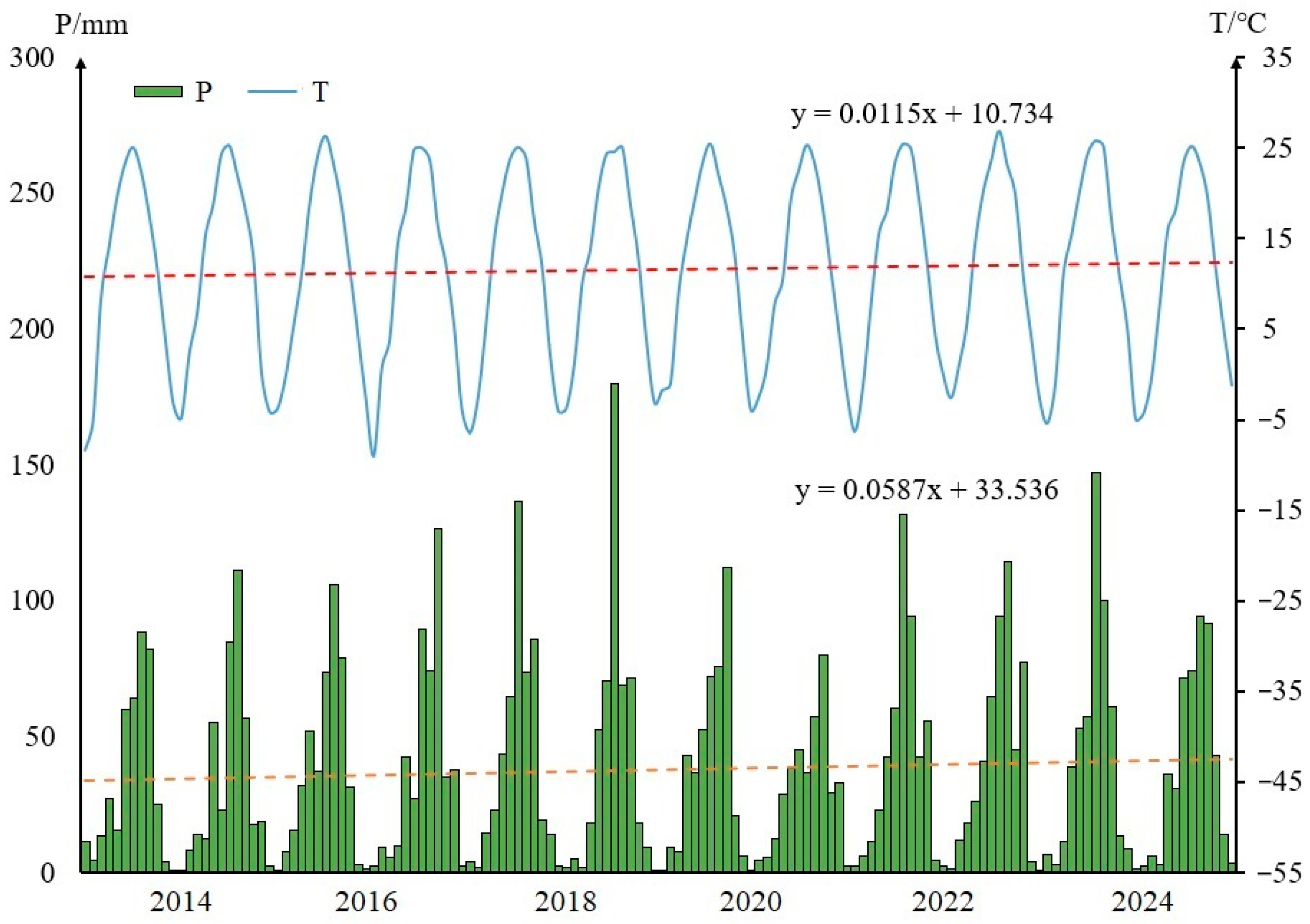
Time series of precipitation(P) and air temperature(T) over the LP were compiled from meteorological station observations to examine the possible climatic controls on TWSC (Figure 9). These climatic variables were used to provide background information for interpreting the temporal behavior of the GLDAS-, GRACE-, GNSS-, and joint-inversion estimates, rather than as independent proof of a single dominant driving mechanism.

In Figure 9, precipitation over the LP shows a slight increasing tendency during 2013–2024, with a net increase of approximately 6.84 mm over the study period. This weak increase indicates that precipitation did not exhibit a substantial long-term decrease during the analysis period. Therefore, the observed TWS depletion cannot be explained by precipitation reduction alone. Instead, it is more likely associated with the combined effects of climatic variability, evapotranspiration change, land-surface conditions, groundwater use, reservoir regulation, and other anthropogenic disturbances.

Air temperature also shows an increasing tendency. In semi-arid and semi-humid regions such as the LP, warming may enhance potential evapotranspiration and vegetation transpiration, thereby increasing water loss from soil and vegetation systems [42]. However, the effect of temperature on TWSC is indirect and depends on vegetation cover, soil properties, water availability, and land-use conditions. Therefore, warming should be regarded as a contributing factor that may amplify water loss, rather than as an independent explanation for the observed TWSC trend.

Comparison between the TWS time series and precipitation records indicates that water storage variations generally respond to seasonal precipitation, but the relationship is not strictly synchronous. Apparent phase differences may arise because individual TWS components, including soil moisture, groundwater, surface water, snow water, and canopy water, have different residence times and response rates to precipitation input. Evapotranspiration, runoff generation, infiltration, groundwater recharge, reservoir operation, and irrigation can further modify the timing and magnitude of regional storage changes. For GRACE, monthly averaging and regional spatial smoothing may also dampen or shift the apparent storage response. For GNSS, any apparent phase difference should not be interpreted as a delayed elastic response of the solid Earth, because elastic loading deformation is expected to occur nearly simultaneously at monthly timescales. Instead, phase differences in GNSS-derived EWH may reflect hydrological storage dynamics, temporal averaging, inversion smoothing, or local deformation effects that are not purely related to elastic hydrological loading.

The thick loess cover of the LP has substantial water-retention capacity and may regulate the seasonal redistribution of water within the near-surface system [43]. Human regulation, including reservoir operation, irrigation, and water diversion, may further alter the timing and magnitude of regional storage changes [44]. These processes help explain why TWS variability does not always follow precipitation directly, even though precipitation remains an important seasonal input.

Overall, the climatic evidence suggests that recent TWSC over the LP is controlled by multiple interacting factors. Precipitation variability explains part of the seasonal fluctuation, while warming-related evapotranspiration, soil water retention, groundwater abstraction, irrigation demand, mining disturbance, ecological restoration, and reservoir regulation may jointly influence the long-term storage trajectory. Because this study does not directly quantify the separate contribution of each factor, the interpretation should be regarded as a process-based explanation of the observed model differences rather than a complete attribution analysis.

4.2. Model-Dependent Discrepancies and Uncertainties

The comparison among GLDAS, GRACE, GNSS, and the joint solution reveals clear model-dependent differences over the LP. GRACE generally indicates stronger long-term TWS depletion than the GLDAS-derived hydrological model benchmark, whereas GNSS-derived EWH shows a weaker long-term trend but stronger seasonal variability. These differences indicate that the four estimates should not be regarded as equivalent representations of the same hydrological signal. Instead, they reflect differences in observation sensitivity, spatial resolution, inversion assumptions, and the degree to which each approach is affected by regional mass redistribution or local deformation.

The stronger depletion signal derived from GRACE may be partly associated with non-TWS mass redistribution within its effective footprint. Soil erosion is one possible contributor. Although sediment control in the Yellow River Basin has improved in recent decades, cumulative sediment export from the LP remains non-negligible. When simplified as a spatially averaged mass deficit over the study area, the reported sediment loss corresponds to an EWH-scale signal of approximately 0.5 mm/yr. This value should be regarded as an order-of-magnitude estimate rather than a direct correction, because erosion, deposition, sediment transport, and sediment retention are spatially heterogeneous. Nevertheless, it suggests that erosion-related mass redistribution may contribute partly to the stronger GRACE-derived depletion signal.

Mining-related mass redistribution may also affect the interpretation of GRACE-based mass change. The LP and its surrounding areas include extensive coal, oil and gas, and bauxite exploitation zones. Based on available production information and a simplified conversion that considers residual backfill and material redistribution, mining-associated mass removal can be expressed as an approximate EWH-scale signal of about 1.9 mm/yr [45]. However, this estimate contains substantial uncertainty because mining intensity, underground void development, backfilling, waste-rock storage, and spatial localization cannot be fully represented by a regional average. Therefore, the mining-related estimate is used only to indicate the possible magnitude of non-TWS mass change, not as a validated correction to GRACE.

In contrast, GNSS-derived EWH may be affected by deformation processes that are not equivalent to elastic hydrological loading. The LP is widely covered by thick loess deposits with metastable pore structures. Under wetting and external loading, loess may undergo collapsible settlement, especially in densely populated or intensively engineered areas. Groundwater extraction may induce aquifer compaction or poroelastic deformation, while mining activity may cause localized or regional subsidence. These processes may be hydrologically triggered or anthropogenically induced, but they do not necessarily represent elastic surface loading caused by TWS change. If such deformation remains in the GNSS vertical displacement series, the converted EWH may contain non-elastic or non-loading components, helping to explain the weaker long-term trend and stronger seasonal variability of the GNSS-based result.

The joint inversion provides a weighted integrated estimate that is closer to the GLDAS-derived hydrological model benchmark than either single geodetic estimate. However, this agreement should be interpreted cautiously. GLDAS is a land-surface hydrological model rather than an observational truth, and the GLDAS-based TWS proxy used here does not fully represent groundwater storage or direct anthropogenic water regulation. To visually explore the sensitivity of the fusion model results to GNSS/GRACE data, we performed a weighted sensitivity analysis on the GNSS/GRACE time series and the combined time series results for 29 stations; the distribution of the sensitivity coefficient K is shown in

Table 3. Distribution of sensitivity coefficient K between the joint solution and the GNSS and GRACE time series at the 29 GNSS stations.

Range of K	GNSS	GRACE
Greater than 1	4	18
Less than 1	25	11

. K is the ratio of the percentage change in the combined model to the percentage change in the independent variable

The weighting-sensitivity analysis further indicates that the GNSS-only inversion has a relatively limited influence on the final joint solution compared with the regional-scale constraint provided by GRACE. Therefore, the joint solution should be interpreted as an integrated estimate that improves consistency with the selected hydrological model benchmark, rather than as direct proof that non-TWS mass signals or non-elastic deformation effects have been completely removed.

The spatial reliability of the GNSS-based inversion is also scale dependent. The revised checkerboard test shows that, at the spatial resolution adopted in this study, the main regional-scale EWH pattern can be recovered reasonably well, indicating that the GNSS network can provide useful constraints for large-scale TWSC interpretation. However, the recovery becomes weaker near the western and northern margins of the LP, where station coverage is relatively sparse. This result supports the use of GNSS-derived information for regional comparison, but it also indicates that fine-scale or marginal spatial features should not be over-interpreted.

Several uncertainties remain. First, the EWH-equivalent estimates of soil erosion and mining are approximate and require further support from spatially explicit sediment budgets, mining production data, land-subsidence observations, and uncertainty analysis. Second, loess collapsibility, aquifer compaction, and poroelastic deformation are discussed as plausible mechanisms, but their individual contributions have not yet been separated from the GNSS signal. Third, although the checkerboard test supports the adopted regional-scale inversion, the sparse GNSS station distribution still limits the recovery of local spatial heterogeneity, especially near the study-region boundaries. Finally, both GRACE and GLDAS have limited ability to resolve fine-scale hydrological variability because of their spatial resolution and preprocessing procedures.

Overall, the model disagreement observed in this study is not only a limitation but also a key scientific result. It indicates that TWSC estimation over the LP is affected by the combined influence of hydrological change, non-TWS mass redistribution, non-elastic ground deformation, and method-dependent uncertainty. The main contribution of this study is therefore not a simple comparison among four TWSC products, but a discrepancy-oriented interpretation of multi-source TWS estimates in a geologically and anthropogenically complex region.

5. Conclusions

This study investigated TWSC over the LP from 2013 to 2024 by integrating GLDAS simulations, GRACE observations, GNSS-derived vertical deformation, and a joint GNSS–GRACE inversion. Unlike previous studies that mainly used multiple datasets for mutual comparison or validation, this study focuses on diagnosing model-dependent discrepancies among hydrological model, gravimetric, deformation-based, and fused TWSC estimates in a geologically and anthropogenically complex region. The main conclusions are as follows.

(1) The four estimates show broadly comparable regional-scale variability, but clear differences exist in trend magnitude, seasonal behavior, and spatial pattern. GRACE indicates a stronger long-term depletion signal, whereas GNSS-derived EWH shows a weaker trend and a more pronounced seasonal component. This result demonstrates that multi-source TWSC estimates over the LP should not be regarded as interchangeable representations of the same hydrological signal. Instead, their discrepancies provide important information on method-dependent sensitivity and regional uncertainty.

(2) Spatially, GLDAS, GRACE, and the joint solution show generally similar large-scale patterns, while the GNSS-derived field exhibits stronger localized variability. This difference is likely related to the sensitivity of GNSS vertical displacement to station-scale and near-surface deformation processes. The revised checkerboard test indicates that, at the spatial resolution adopted in this study, the GNSS inversion can recover the main regional-scale EWH pattern, although recovery becomes weaker near the margins of the study region. Therefore, GNSS-based TWSC inversion over the LP can provide useful regional constraints, but local-scale features should be interpreted cautiously, particularly in areas affected by collapsible loess, groundwater withdrawal, mining activity, and other local deformation sources.

(3) Climatic factors contribute to the seasonal variability of regional water storage, but they cannot fully explain the long-term differences among the datasets. Precipitation over the study period does not show a substantial decreasing tendency, while warming may enhance evapotranspiration and soil moisture loss. Human activities, including irrigation, groundwater abstraction, mining, reservoir regulation, and ecological restoration, may further modify the regional water balance. This indicates that TWSC over the LP is controlled by coupled climatic, hydrological, geological, and anthropogenic processes rather than by precipitation change alone.

(4) Soil erosion and mining-related mass redistribution may contribute additional non-TWS mass signals to GRACE-based estimates, whereas loess collapsibility, aquifer compaction, poroelastic deformation, and mining-induced subsidence may affect GNSS-derived EWH. The EWH-equivalent estimates for soil erosion and mining provide an approximate indication of their possible magnitude, but they should not be interpreted as complete corrections without spatially explicit datasets and uncertainty assessment. This highlights the need to distinguish true hydrological storage change from non-TWS mass redistribution and non-loading deformation in complex loess regions.

(5) The joint inversion yields results closer to the GLDAS-derived hydrological model benchmark than either GRACE or GNSS alone. However, GLDAS is not an absolute reference because the GLDAS-based TWS proxy does not fully represent groundwater storage or direct human water regulation. The weighting-sensitivity analysis further indicates that the GNSS-only inversion has a relatively limited influence on the final joint solution compared with the regional-scale constraint provided by GRACE. Therefore, the joint solution should be interpreted as a weighted integrated estimate that improves consistency with the selected hydrological model benchmark, rather than as direct proof that non-TWS mass change or non-elastic deformation has been completely removed.

Overall, the main contribution of this study is not simply the comparison of four TWSC models, but the development of a discrepancy-oriented framework for interpreting multi-source TWS estimates over the LP. By combining temporal comparison, spatial analysis, checkerboard testing, weighting-sensitivity assessment, and discussion of non-hydrological mass and deformation effects, this study provides a more cautious and physically interpretable basis for applying GRACE-, GNSS-, GLDAS-, and joint GNSS-GRACE inversion approaches in geologically and anthropogenically complex regions. Future studies should incorporate independent constraints, such as groundwater-level observations, InSAR-derived land subsidence, sediment transport records, mining activity maps, reservoir storage data, evapotranspiration products, and land-use information, to better separate hydrological storage change from non-loading deformation and non-TWS mass redistribution.

References

1. Feng, W.; Zhong, M.; Lemoine, J.-M.; Biancale, R.; Hsu, H.-T.; Xia, J. Evaluation of groundwater depletion in North China using the Gravity Recovery and Climate Experiment (GRACE) data and ground-based measurements. Water Resour. Res. 2013, 49, 2110–2118. [Google Scholar] [CrossRef] [Scilit]
2. An, L.; Wang, J.; Huang, J.; Pokhrel, Y.; Hugonnet, R.; Wada, Y.; Cáceres, D.; Schmied, H.M.; Song, C.; Berthier, E.; et al. Divergent causes of terrestrial water storage declines between drylands and humid regions globally. Geophys. Res. Lett. 2021, 48, e2021GL095035. [Google Scholar] [CrossRef] [Scilit]
3. Majumdar, S.; Smith, R.; Butler, J.J.; Lakshmi, V. Groundwater withdrawal prediction using integrated multi-temporal remote sensing datasets and machine learning. Water Resour. Res. 2020, 56, e2020WR028059. [Google Scholar] [CrossRef] [Scilit]
4. Tapley, B.D.; Bettadpur, S.; Ries, J.C.; Thompson, P.F.; Watkins, M.M. GRACE measurements of mass variability in the Earth system. Science 2004, 305, 503–505. [Google Scholar] [CrossRef] [Scilit] [PubMed]
5. Scanlon, B.R.; Rateb, A.; Pool, D.R.; Sanford, W.; Save, H.; Sun, A.; Long, D.; Fuchs, B. Effects of climate and irrigation on GRACE-based estimates of water storage changes in major U.S. aquifers. Environ. Res. Lett. 2021, 16, 094009. [Google Scholar] [CrossRef] [Scilit]
6. Masood, A.; Tariq, M.A.U.R.; Hashmi, M.Z.U.R.; Waseem, M.; Sarwar, M.K.; Ali, W.; Farooq, R.; Almazroui, M.; Ng, A.W.M. An overview of groundwater monitoring through point-to satellite-based techniques. Water 2022, 14, 565. [Google Scholar] [CrossRef] [Scilit]
7. Chen, J.L.; Wilson, C.R.; Famiglietti, J.S.; Rodell, M. Spatial sensitivity of the Gravity Recovery and Climate Experiment (GRACE) time-variable gravity observations. J. Geophys. Res. Solid Earth 2005, 110, B08406. [Google Scholar] [CrossRef] [Scilit]
8. White, A.M.; Gardner, W.P.; Borsa, A.A.; Argus, D.F.; Martens, H.R. A review of GNSS/GPS in hydrogeodesy: Hydrologic loading applications and their implications for water resource research. Water Resour. Res. 2022, 58, e2022WR032078. [Google Scholar] [CrossRef] [Scilit] [PubMed]
9. Li, W.; Dong, J.; Wang, W.; Zhong, Y.; Zhang, C.; Wen, H.; Liu, H.; Guo, Q.; Yao, G. The crustal vertical deformation driven by terrestrial water load from 2010 to 2014 in Shaanxi–Gansu–Ningxia region based on GRACE and GNSS. Water 2022, 14, 964. [Google Scholar] [CrossRef] [Scilit]
10. Feng, W.; Shum, C.K.; Zhong, M.; Pan, Y. Groundwater storage changes in China from satellite gravity: An overview. Remote Sens. 2018, 10, 674. [Google Scholar] [CrossRef] [Scilit]
11. Zhou, J.; Cui, L.; Li, Y.; Yao, C.; Meng, J.; Zou, Z.; Lu, Y. GRACE/GFO and Swarm Observation Analysis of the 2023–2024 Extreme Drought in the Amazon River Basin. Remote Sens. 2025, 17, 2765. [Google Scholar] [CrossRef] [Scilit]
12. Kusche, J.; Schrama, O.J.E. Surface mass redistribution inversion from global GPS deformation and Gravity Recovery and Climate Experiment (GRACE) gravity data. J. Geophys. Res. Solid Earth 2005, 110, B09409. [Google Scholar] [CrossRef] [Scilit]
13. Hao, M.; Li, Y.; Wang, Q.; Zhuang, W.; Qu, W. Present-Day Crustal Deformation Within the Western Qinling Mountains and Its Kinematic Implications. Remote Sens. 2021, 13, 1–19. [Google Scholar] [CrossRef] [Scilit]
14. Pan, Y.; Chen, R.; Yi, S.; Wang, W.; Ding, H.; Shen, W.; Chen, L. Contemporary mountain-building of the Tianshan and its relevance to geodynamics constrained by integrating GPS and GRACE measurements. J. Geophys. Res. Solid Earth 2019, 124, 12171–12188. [Google Scholar] [CrossRef] [Scilit]
15. Su, G.; Zhan, W. Abnormal depletion of terrestrial water storage and crustal uplift owing to the 2019 drought in Yunnan, China. Geophys. J. Int. 2022, 231, 108–117. [Google Scholar] [CrossRef] [Scilit]
16. Carlson, G.; Werth, S.; Shirzaei, M. Joint inversion of GNSS and GRACE for terrestrial water storage change in California. J. Geophys. Res. Solid Earth 2022, 127, e2021JB023135. [Google Scholar] [CrossRef] [Scilit] [PubMed]
17. Wang, Z.; Xu, M.; Penny, G.; Hu, H.; Zhang, X.; Tian, S. Impact of revegetation and agricultural intensification on water storage variation in the Yellow River Basin. J. Hydrol. 2024, 635, 131218. [Google Scholar] [CrossRef] [Scilit]
18. Cao, Y.; Nan, Z.; Cheng, G. GRACE Gravity Satellite Observations of Terrestrial Water Storage Changes for Drought Characterization in the Arid Land of Northwestern China. Remote Sens. 2015, 7, 1021–1047. [Google Scholar] [CrossRef] [Scilit]
19. Purdy, A.J.; David, C.H.; Sikder, M.S.; Reager, J.T.; Chandanpurkar, H.A.; Jones, N.L.; Matin, M.A. An open-source tool to facilitate the processing of GRACE observations and GLDAS outputs: An evaluation in Bangladesh. Front. Environ. Sci. 2019, 7, 155. [Google Scholar] [CrossRef] [Scilit]
20. Rodell, M.; Houser, P.R.; Jambor, U.; Gottschalck, J.; Mitchell, K.; Meng, C.; Arsenault, K.; Cosgrove, B.; Radakovich, J.; Bosilovich, M.; et al. The global land data assimilation system. Bull. Am. Meteorol. Soc. 2004, 85, 381–394. [Google Scholar] [CrossRef] [Scilit]
21. Long, D.; Pan, Y.; Zhou, J.; Chen, Y.; Hou, X.; Hong, Y.; Scanlon, B.R.; Longuevergne, L. Global analysis of spatiotemporal variability in merged total water storage changes using multiple GRACE products and global hydrological models. Remote Sens. Environ. 2017, 192, 198–216. [Google Scholar] [CrossRef] [Scilit]
22. Rodell, M.; Famiglietti, J.S.; Wiese, D.N.; Reager, J.T.; Beaudoing, H.K.; Landerer, F.W.; Lo, M.-H. Emerging trends in global freshwater availability. Nature 2018, 557, 651–659. [Google Scholar] [CrossRef] [Scilit] [PubMed]
23. Velicogna, I.; Wahr, J. Acceleration of Greenland ice mass loss in spring 2004. Nature 2006, 443, 329–331. [Google Scholar] [CrossRef] [Scilit] [PubMed]
24. Sun, Z.; Long, D.; Yang, W.; Li, X.; Pan, Y. Reconstruction of GRACE data on changes in total water storage over the global land surface and 60 basins. Water Resour. Res. 2020, 56, e2019WR026250. [Google Scholar] [CrossRef] [Scilit]
25. Chanu, C.S.; Munagapati, H.; Tiwari, V.M.; Kumar, A.; Elango, L. Use of GRACE time-series data for estimating groundwater storage at small scale. J. Earth Syst. Sci. 2020, 129, 215. [Google Scholar] [CrossRef] [Scilit]
26. Xu, P.; Jiang, T.; Zhang, C.; Rui, M.; Liu, Y. Data filling of terrestrial water storage anomaly during the gap period of GRACE/GRACE-FO: A case study of global typical basins. Chin. J. Geophys. 2021, 64, 3048–3067. [Google Scholar] [CrossRef]
27. Shi, T.; Liu, X.; Mu, D.; Li, C.; Guo, J.; Xing, Y. Reconstructing gap data between GRACE and GRACE-FO based on multi-layer perceptron and analyzing terrestrial water storage changes in the Yellow River basin. Chin. J. Geophys. 2022, 65, 2448–2463. [Google Scholar] [CrossRef]
28. Xie, J.; Xu, Y.; Wang, Y.; Gu, H.; Wang, F.; Pan, S. Influences of climatic variability and human activities on terrestrial water storage variations across the Yellow River basin in the recent decade. J. Hydrol. 2019, 579, 124218. [Google Scholar] [CrossRef] [Scilit]
29. Argus, F.D.; Martens, H.R.; Borsa, A.A.; Knappe, E.; Wiese, D.N.; Alam, S.; Anderson, M.; Khatiwada, A.; Lau, N.; Peidou, A.; et al. Subsurface water flux in California’s central valley and its source watershed from space geodesy. Geophys. Res. Lett. 2022, 49, e2022GL099583. [Google Scholar] [CrossRef] [Scilit]
30. Matthews, M.V.; Segall, P. Estimation of depth-dependent fault slip from measured surface deformation with application to the 1906 San Francisco earthquake. J. Geophys. Res. Solid Earth 1993, 98, 12153–12163. [Google Scholar] [CrossRef] [Scilit]
31. Qian, A.; Yi, S.; Li, F.; Su, B.; Sun, G.; Liu, X. Evaluation of the Consistency of Three GRACE Gap-Filling Data. Remote Sens. 2022, 14, 3916. [Google Scholar] [CrossRef] [Scilit]
32. Baur, O. On the Computation of Mass-Change Trends from GRACE Gravity Field Time-Series. Remote Sens. 2012, 61, 120–128. [Google Scholar] [CrossRef] [Scilit]
33. Ghaderpour, E. JUST: MATLAB and Python Software for Change Detection and Time Series Analysis. GPS Solut. 2021, 25, 85. [Google Scholar] [CrossRef] [Scilit]
34. Argus, D.F.; Landerer, F.W.; Wiese, D.N.; Martens, H.R.; Fu, Y.; Famiglietti, J.S.; Thomas, B.F.; Farr, T.G.; Moore, A.W.; Watkins, M.M. Sustained Water Loss in California’s Mountain Ranges During Severe Drought from 2012 to 2015 Inferred from GPS. J. Geophys. Res. Solid Earth 2017, 122, 10559–10585. [Google Scholar] [CrossRef] [Scilit]
35. Yan, H.; Chen, W.; Zhu, Y.; Zhang, W.; Zhong, M. Contributions of Thermal Expansion of Monuments and Nearby Bedrock to Observed GPS Height Changes. Geophys. Res. Lett. 2009, 36, L13301. [Google Scholar] [CrossRef] [Scilit]
36. Argus, D.F.; Fu, Y.; Landerer, F.W. Seasonal Variation in Total Water Storage in California Inferred from GPS Observations of Vertical Land Motion. Geophys. Res. Lett. 2014, 41, 1971–1980. [Google Scholar] [CrossRef] [Scilit]
37. Jiang, Z.; Hsu, Y.-J.; Yuan, L.; Huang, D. Monitoring Time-Varying Terrestrial Water Storage Changes Using Daily GNSS Measurements in Yunnan, Southwest China. Remote Sens. Environ. 2021, 254, 112249. [Google Scholar] [CrossRef] [Scilit]
38. Zhu, W.; Xu, K.; Darve, E.; Beroza, G.C. A General Approach to Seismic Inversion with Automatic Differentiation. Comput. Geosci. 2021, 151, 104751. [Google Scholar] [CrossRef] [Scilit]
39. Scanlon, B.R.; Zhang, Z.; Rateb, A.; Sun, A.; Wiese, D.; Save, H.; Famiglietti, J.S. Tracking Seasonal Fluctuations in Land Water Storage Using Global Models and GRACE Satellites. Geophys. Res. Lett. 2019, 46, 5254–5264. [Google Scholar] [CrossRef] [Scilit]
40. Wang, Y.; Zhao, W.; Wang, S.; Feng, X.; Liu, Y. Yellow River Water Rebalanced by Human Regulation. Sci. Rep. 2019, 9, 9707. [Google Scholar] [CrossRef] [Scilit] [PubMed]
41. Wang, S.Y.; Li, J.; Chen, J.; Hu, X.G. On the Improvement of Mass Load Inversion with GNSS Horizontal Deformation: A Synthetic Study in Central China. J. Geophys. Res. Solid Earth 2022, 127, e2021JB023696. [Google Scholar] [CrossRef] [Scilit]
42. Huang, J.; Guan, X.; Ji, F. Enhanced Cold-Season Warming in Semi-Arid Regions. Atmos. Chem. Phys. 2012, 12, 5391–5398. [Google Scholar] [CrossRef] [Scilit]
43. Li, Z.; Deng, X.; Yin, F.; Yang, C. Analysis of Climate and Land Use Changes Impacts on Land Degradation in the North China Plain. Adv. Meteorol. 2015, 2015, 976370. [Google Scholar] [CrossRef] [Scilit]
44. Long, D.; Scanlon, B.R.; Longuevergne, L.; Sun, A.-Y.; Fernando, D.N.; Save, H. GRACE Satellites Monitor Large Depletion in Water Storage in Response to the 2011 Drought in Texas. Geophys. Res. Lett. 2013, 40, 3395–3401. [Google Scholar] [CrossRef] [Scilit]
45. Wang, L.L. Inversion and Main Influencing Factors of Water Storage Change on the Loess Plateau Based on GRACE Gravity Data. Master’s Thesis, East China University of Technology, Nanchang, China, 2024. (In Chinese) [Google Scholar] [CrossRef]
Figure 1. Schematic diagram of the methodology.
Remotesensing 18 02732 g001
Figure 2. Spatial distribution of the study area and GNSS stations.
Remotesensing 18 02732 g002
Figure 3. Results of checkerboard test (a,c,e) show the raw input signal, GNSS inversion results, and joint inversion results, respectively, for a 2° × 2° grid; (b,d,f) show the raw input signal, GNSS inversion results, and joint inversion results, respectively, for a 1° × 1° grid. The black dots indicate the locations of GNSS stations.
Remotesensing 18 02732 g003
Figure 4. SSA decomposition of the 2013–2024 TWS expressed as EWH time series over the LP. The original series (black) is separated into a long-term trend (red dashed), a seasonal component (blue), and a residual component (yellow). Panels show results for (a) GLDAS, (b) GRACE, (c) GNSS, and (d) the joint model.
Remotesensing 18 02732 g004
Figure 5. Spatial distribution of TWS expressed as EWH derived from the GLDAS model for January 2016 (a), July 2016 (b), January 2020 (c), July 2020 (d), January 2024 (e), and July 2024 (f).
Remotesensing 18 02732 g005
Figure 6. Spatial distribution of TWS expressed as EWH derived from the GRACE model for January 2016 (a), July 2016 (b), January 2020 (c), July 2020 (d), January 2024 (e), and July 2024 (f).
Remotesensing 18 02732 g006
Figure 7. Spatial distribution of TWS expressed as EWH derived from the GNSS model for January 2016 (a), July 2016 (b), January 2020 (c), July 2020 (d), January 2024 (e), and July 2024 (f).
Remotesensing 18 02732 g007
Figure 8. Spatial distribution of TWS expressed as EWH derived from the joint inversion model for January 2016 (a), July 2016 (b), January 2020 (c), July 2020 (d), January 2024 (e), and July 2024 (f).
Remotesensing 18 02732 g008
Figure 9. Time series of precipitation and air temperature over the LP from 2013 to 2024 derived from meteorological station observations. The dotted line represents the fitted trend line.
Remotesensing 18 02732 g009