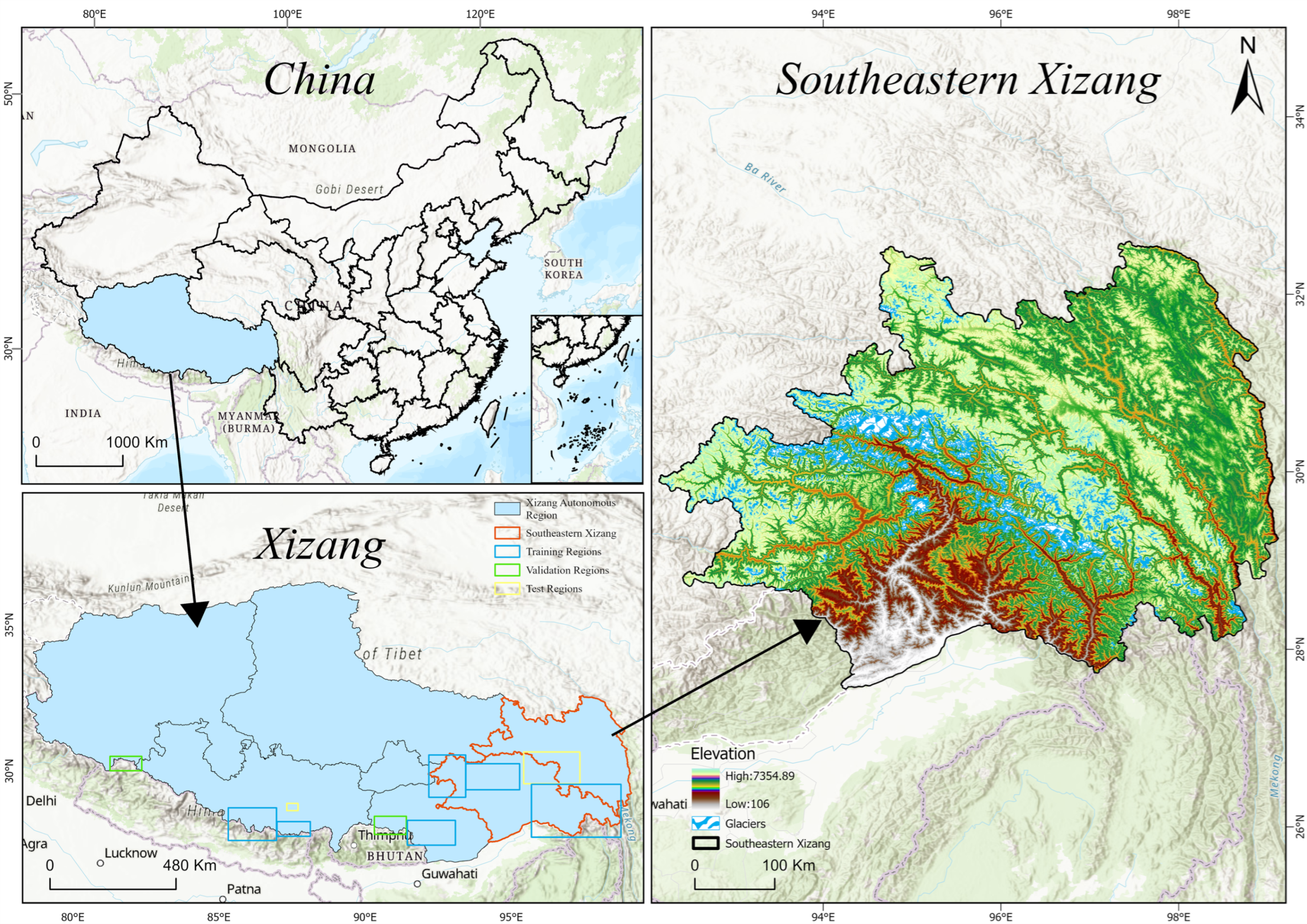
Figure 1.
Location and environmental setting of the study area in southeastern Tibet, together with the spatial distribution of the ten sample regions used for dataset construction and partitioning. Black arrows indicate the nested geographic relationship from China to Xizang and from Xizang to southeastern Xizang. The national boundary shown in the China inset was based on the standard map with approval number GS (2024) 0650.
Figure 1.
Location and environmental setting of the study area in southeastern Tibet, together with the spatial distribution of the ten sample regions used for dataset construction and partitioning. Black arrows indicate the nested geographic relationship from China to Xizang and from Xizang to southeastern Xizang. The national boundary shown in the China inset was based on the standard map with approval number GS (2024) 0650.
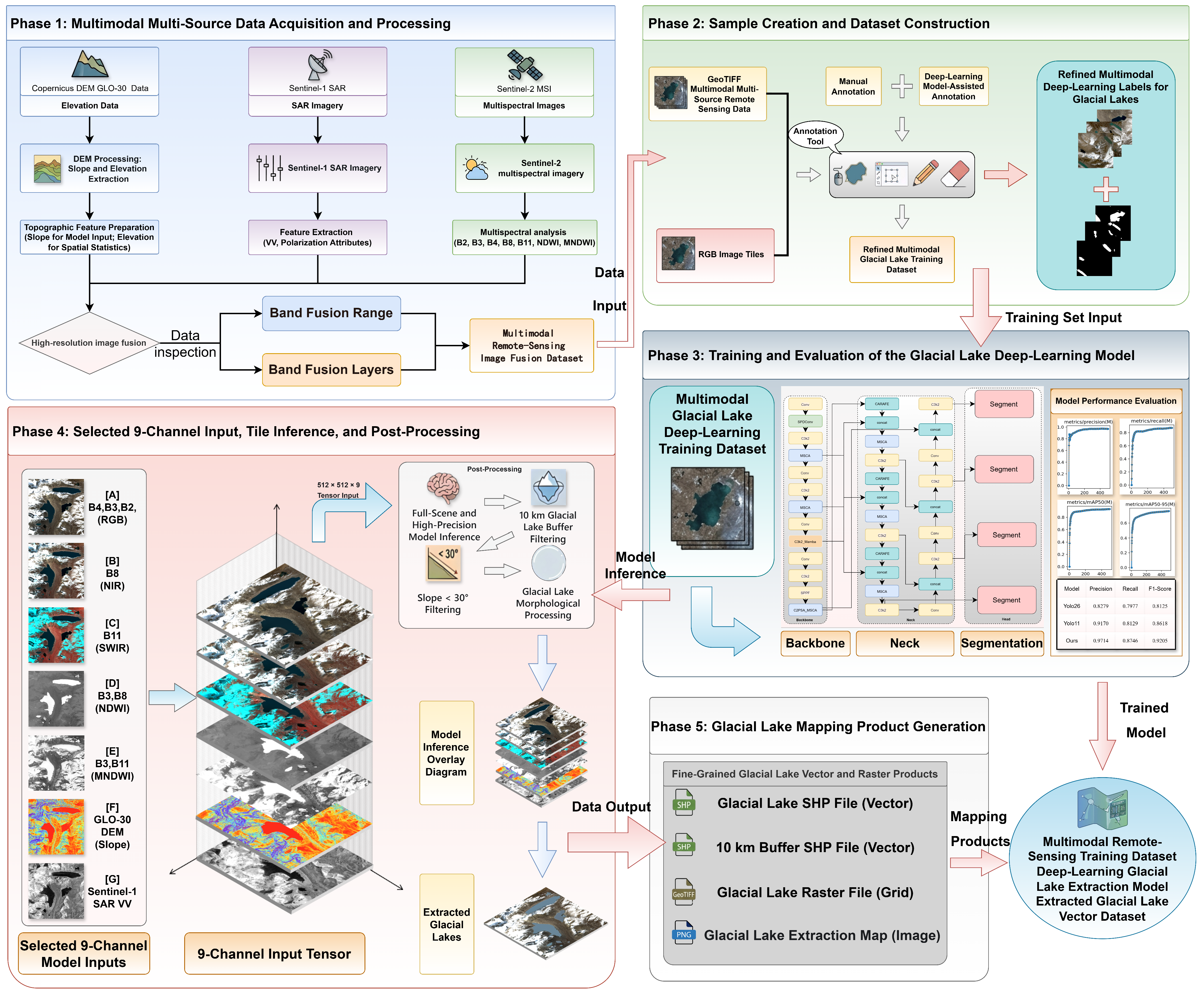
Figure 2.
Overall workflow of the proposed multimodal remote sensing framework for glacial lake extraction and regional inventory generation in southeastern Tibet. The framework comprises five phases: (1) acquisition and preprocessing of Copernicus DEM GLO-30, Sentinel-1 SAR, and Sentinel-2 MSI data, followed by band fusion; (2) sample creation through the combination of manual and deep-learning-model-assisted annotation; (3) training and evaluation of the glacial lake segmentation model; (4) nine-channel tile inference and post-processing, including glacier-buffer filtering, slope filtering, and morphological processing; and (5) generation of glacial lake vector, raster, and mapping products. Black arrows indicate sequential data-processing steps and network feature propagation within a phase; light-gray arrows indicate local annotation and post-processing operations; red arrows indicate the transfer of datasets, labels, training inputs, trained models, inference results, and mapping products across the major workflow stages; and blue arrows indicate the transfer of multimodal input tensors into the network and the inference/output flow in Phases 3 and 4. Plus signs indicate the integration of manual and model-assisted annotation and the combination of image tiles with their corresponding label masks.
Figure 2.
Overall workflow of the proposed multimodal remote sensing framework for glacial lake extraction and regional inventory generation in southeastern Tibet. The framework comprises five phases: (1) acquisition and preprocessing of Copernicus DEM GLO-30, Sentinel-1 SAR, and Sentinel-2 MSI data, followed by band fusion; (2) sample creation through the combination of manual and deep-learning-model-assisted annotation; (3) training and evaluation of the glacial lake segmentation model; (4) nine-channel tile inference and post-processing, including glacier-buffer filtering, slope filtering, and morphological processing; and (5) generation of glacial lake vector, raster, and mapping products. Black arrows indicate sequential data-processing steps and network feature propagation within a phase; light-gray arrows indicate local annotation and post-processing operations; red arrows indicate the transfer of datasets, labels, training inputs, trained models, inference results, and mapping products across the major workflow stages; and blue arrows indicate the transfer of multimodal input tensors into the network and the inference/output flow in Phases 3 and 4. Plus signs indicate the integration of manual and model-assisted annotation and the combination of image tiles with their corresponding label masks.

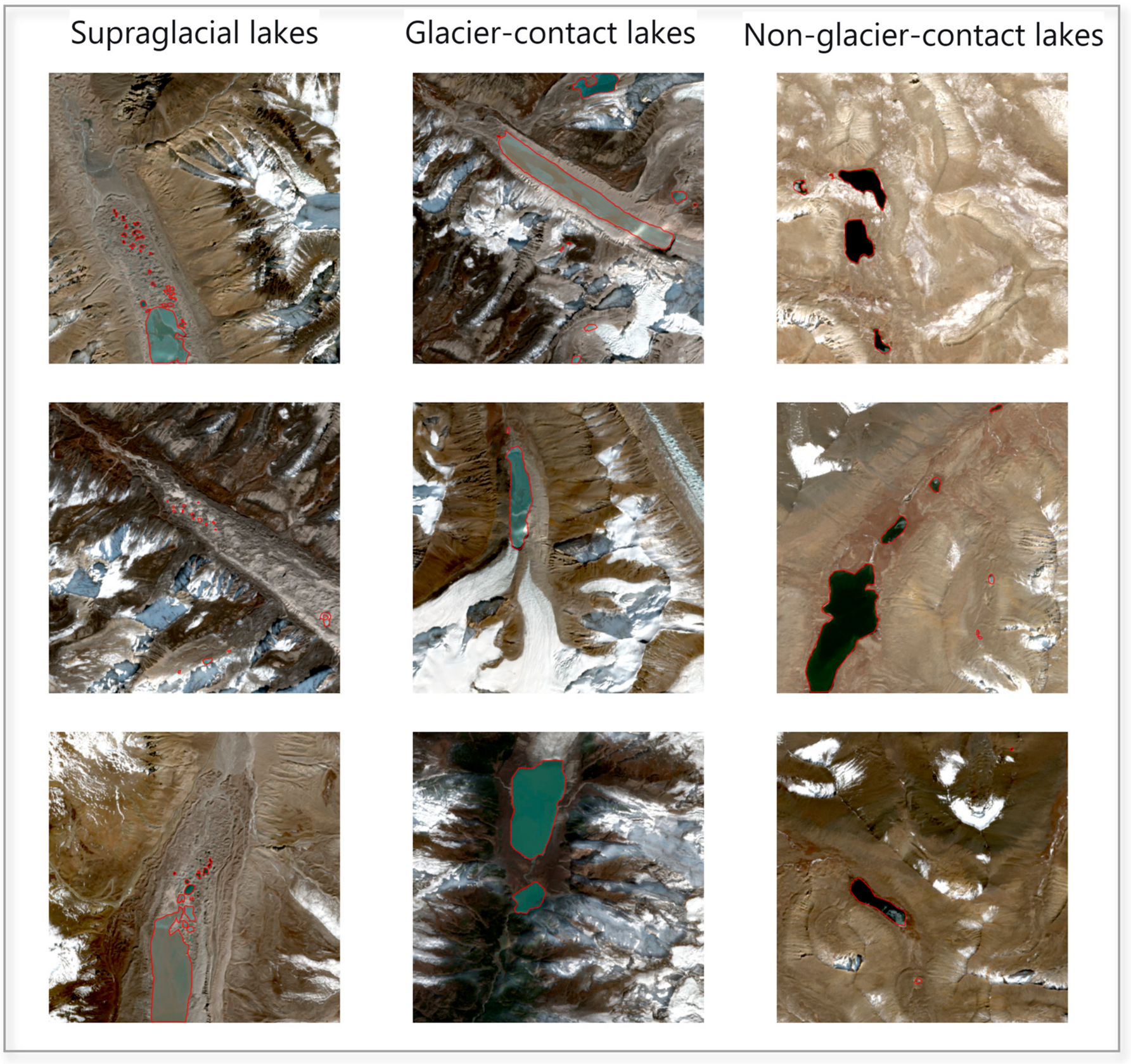
Figure 3.
Representative annotated samples illustrating three glacial lake settings: supraglacial lakes, glacier-contact lakes, and non-glacier-contact lakes. Red outlines delineate the manually annotated glacial lake instance boundaries used as reference labels.
Figure 3.
Representative annotated samples illustrating three glacial lake settings: supraglacial lakes, glacier-contact lakes, and non-glacier-contact lakes. Red outlines delineate the manually annotated glacial lake instance boundaries used as reference labels.
Figure 4.
Architecture of the enhanced YOLO11 glacial lake segmentation network. Yellow blocks denote standard convolutional, C3k2/C3k, and downsampling operations; green, blue, cyan, orange, and purple blocks denote SPDConv, MSCA/C2PSA_MSCA, CARAFE upsampling, C3k2_Mamba/bottleneck, and SPPF operations, respectively. Pink blocks denote feature concatenation, and light-blue blocks denote segmentation heads. Black arrows indicate feature propagation, the circled plus sign indicates residual addition, and dashed outlines group the input/output examples and the backbone, neck, and head components.
Figure 4.
Architecture of the enhanced YOLO11 glacial lake segmentation network. Yellow blocks denote standard convolutional, C3k2/C3k, and downsampling operations; green, blue, cyan, orange, and purple blocks denote SPDConv, MSCA/C2PSA_MSCA, CARAFE upsampling, C3k2_Mamba/bottleneck, and SPPF operations, respectively. Pink blocks denote feature concatenation, and light-blue blocks denote segmentation heads. Black arrows indicate feature propagation, the circled plus sign indicates residual addition, and dashed outlines group the input/output examples and the backbone, neck, and head components.
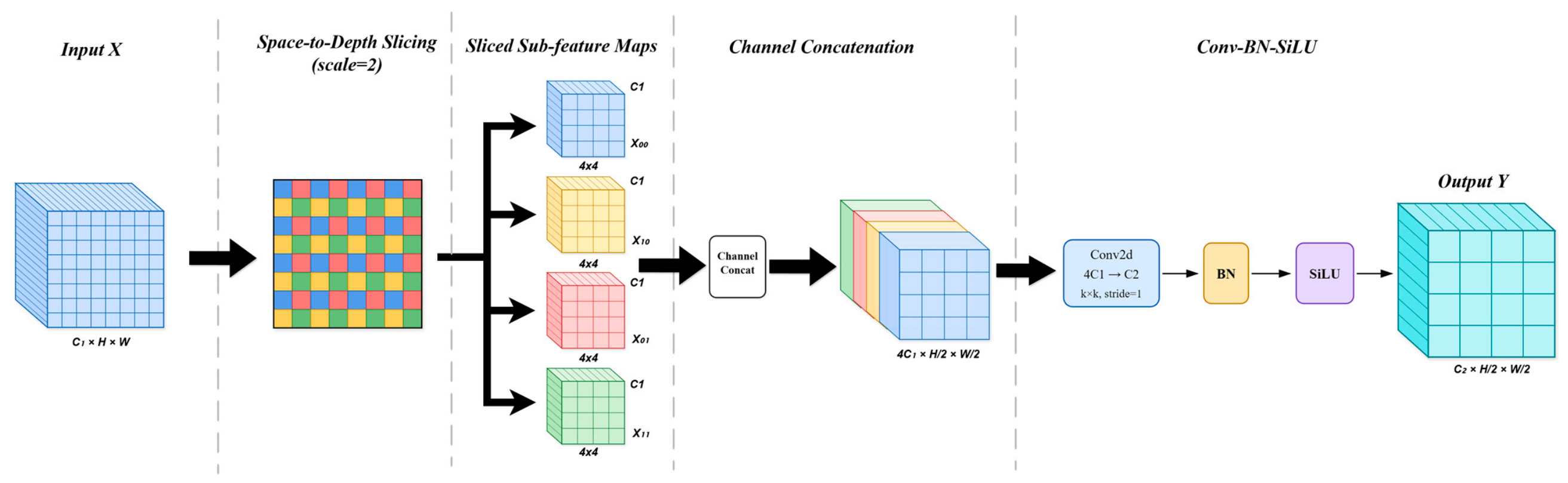
Figure 5.
Structure of the SPDConv module. Blue, yellow, red, and green cells denote the four interleaved spatial offsets sampled from the input feature map, yielding X00, X10, X01, and X11, respectively. The four sub-feature maps are concatenated along the channel dimension and then processed by convolution, batch normalization (BN), and SiLU activation to produce the output feature Y. Black arrows indicate the processing sequence, and gray dashed lines separate the major processing stages.
Figure 5.
Structure of the SPDConv module. Blue, yellow, red, and green cells denote the four interleaved spatial offsets sampled from the input feature map, yielding X00, X10, X01, and X11, respectively. The four sub-feature maps are concatenated along the channel dimension and then processed by convolution, batch normalization (BN), and SiLU activation to produce the output feature Y. Black arrows indicate the processing sequence, and gray dashed lines separate the major processing stages.
Figure 6.
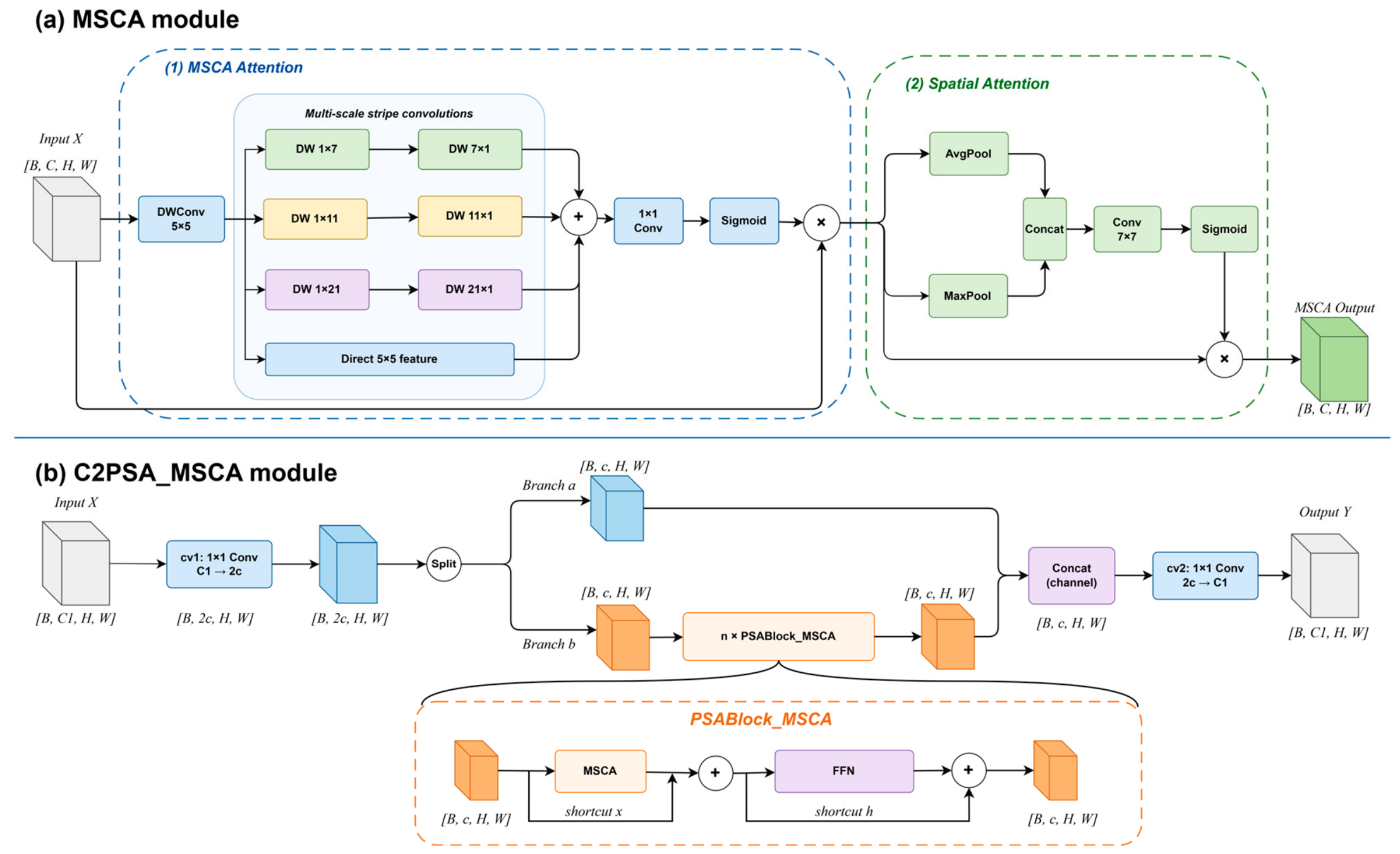
Structures of the (a) MSCA and (b) C2PSA_MSCA modules. In (a), the blue dashed region denotes multi-scale convolutional attention and the green dashed region denotes spatial attention. Green, yellow, and purple blocks distinguish the strip-convolution branches with kernel extents of 7, 11, and 21, respectively, while blue blocks denote the direct and convolutional feature paths. In (b), blue and orange feature maps distinguish the two split branches, and the orange dashed box denotes the repeated PSABlock_MSCA unit. Circled plus and multiplication signs denote elementwise addition and multiplication, respectively, and arrows indicate feature flow.
Figure 6.
Structures of the (a) MSCA and (b) C2PSA_MSCA modules. In (a), the blue dashed region denotes multi-scale convolutional attention and the green dashed region denotes spatial attention. Green, yellow, and purple blocks distinguish the strip-convolution branches with kernel extents of 7, 11, and 21, respectively, while blue blocks denote the direct and convolutional feature paths. In (b), blue and orange feature maps distinguish the two split branches, and the orange dashed box denotes the repeated PSABlock_MSCA unit. Circled plus and multiplication signs denote elementwise addition and multiplication, respectively, and arrows indicate feature flow.
Figure 7.
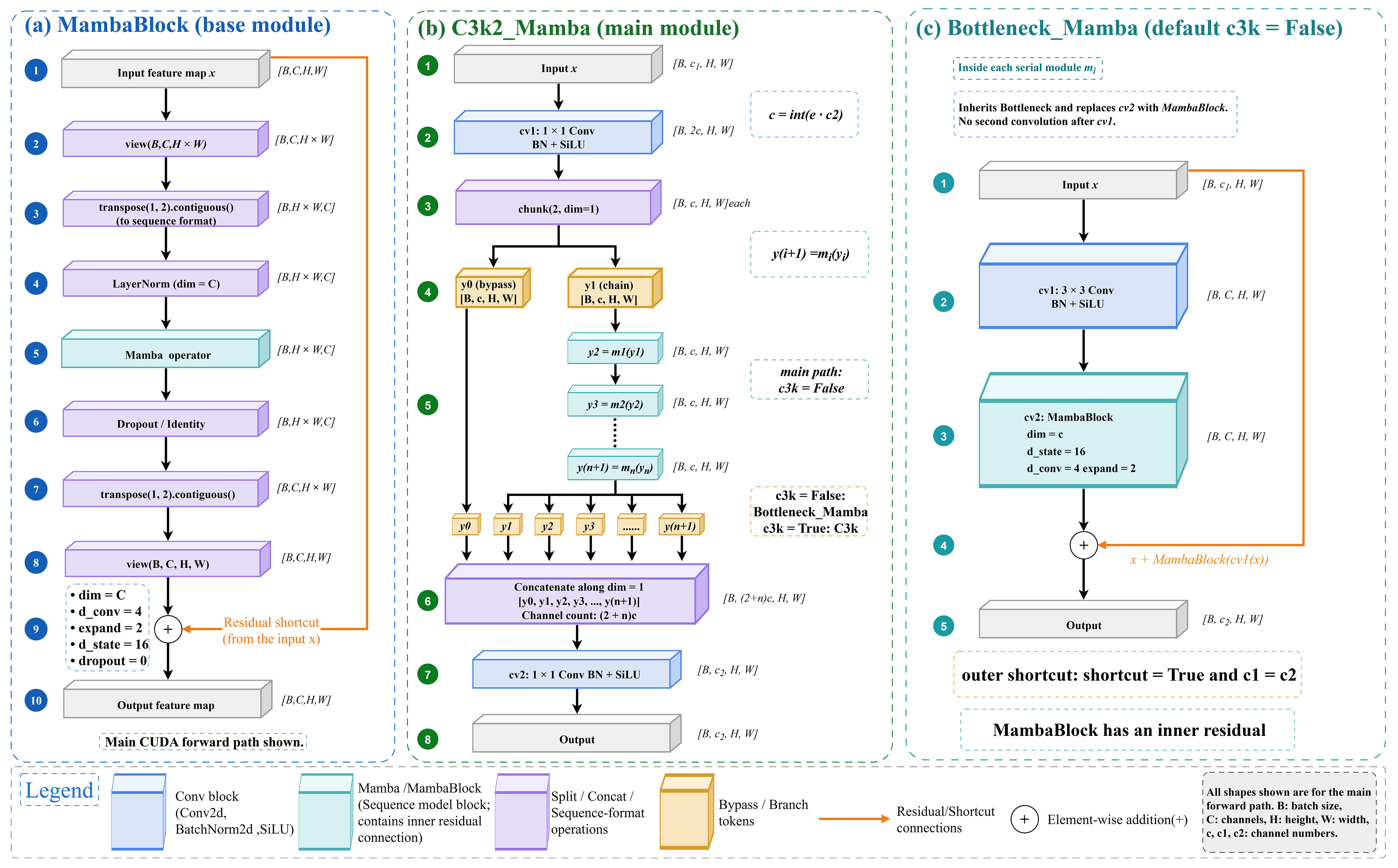
Structure of the C3k2_Mamba module.
Figure 7.
Structure of the C3k2_Mamba module.
Figure 8.
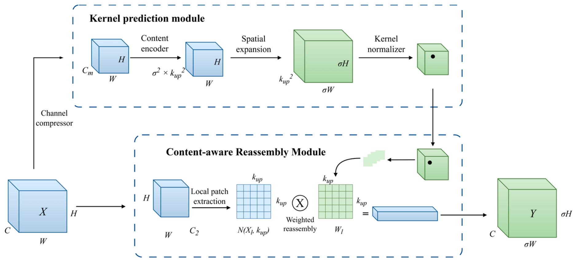
Structure of the CARAFE module. Blue feature maps denote the input and intermediate features used for channel compression and local patch extraction, whereas green feature maps denote the predicted reassembly kernels and the upsampled output. The upper and lower dashed boxes identify the kernel-prediction and content-aware reassembly modules, respectively. Black arrows indicate feature flow, and the circled multiplication symbol denotes the weighted reassembly of each local patch using the normalized kernel weights.
Figure 8.
Structure of the CARAFE module. Blue feature maps denote the input and intermediate features used for channel compression and local patch extraction, whereas green feature maps denote the predicted reassembly kernels and the upsampled output. The upper and lower dashed boxes identify the kernel-prediction and content-aware reassembly modules, respectively. Black arrows indicate feature flow, and the circled multiplication symbol denotes the weighted reassembly of each local patch using the normalized kernel weights.
Figure 9.
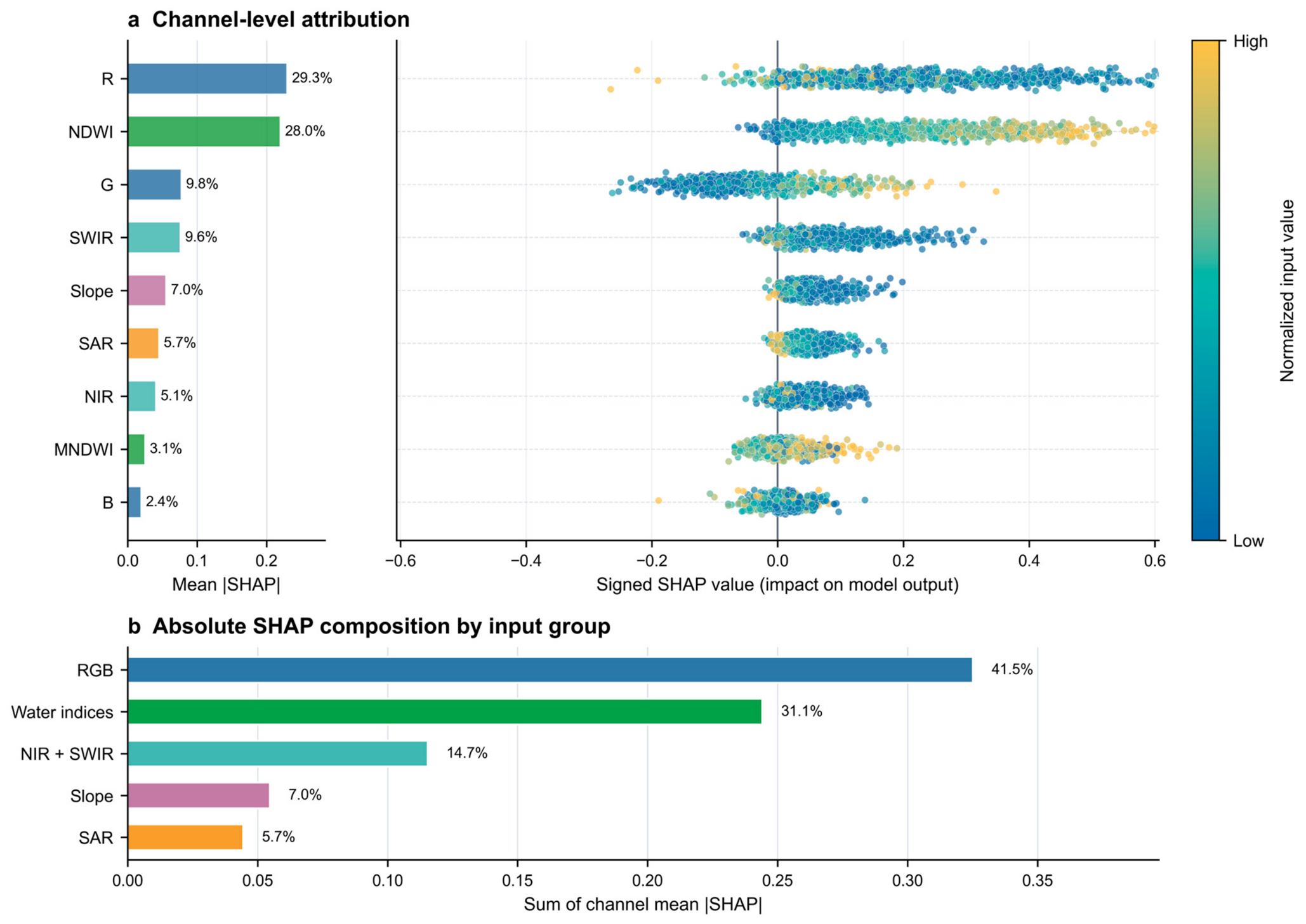
Channel-level and input-group SHAP attribution of the complete 9-channel model based on 1000 validation samples. (a) Mean absolute SHAP values and relative contributions of the nine input channels, together with the sample-level signed SHAP distributions. Dot colors indicate normalized input values within each channel, ranging from low to high. (b) Absolute SHAP composition of the five predefined input groups, calculated by summing the mean absolute SHAP values of their constituent channels.
Figure 9.
Channel-level and input-group SHAP attribution of the complete 9-channel model based on 1000 validation samples. (a) Mean absolute SHAP values and relative contributions of the nine input channels, together with the sample-level signed SHAP distributions. Dot colors indicate normalized input values within each channel, ranging from low to high. (b) Absolute SHAP composition of the five predefined input groups, calculated by summing the mean absolute SHAP values of their constituent channels.
Figure 10.
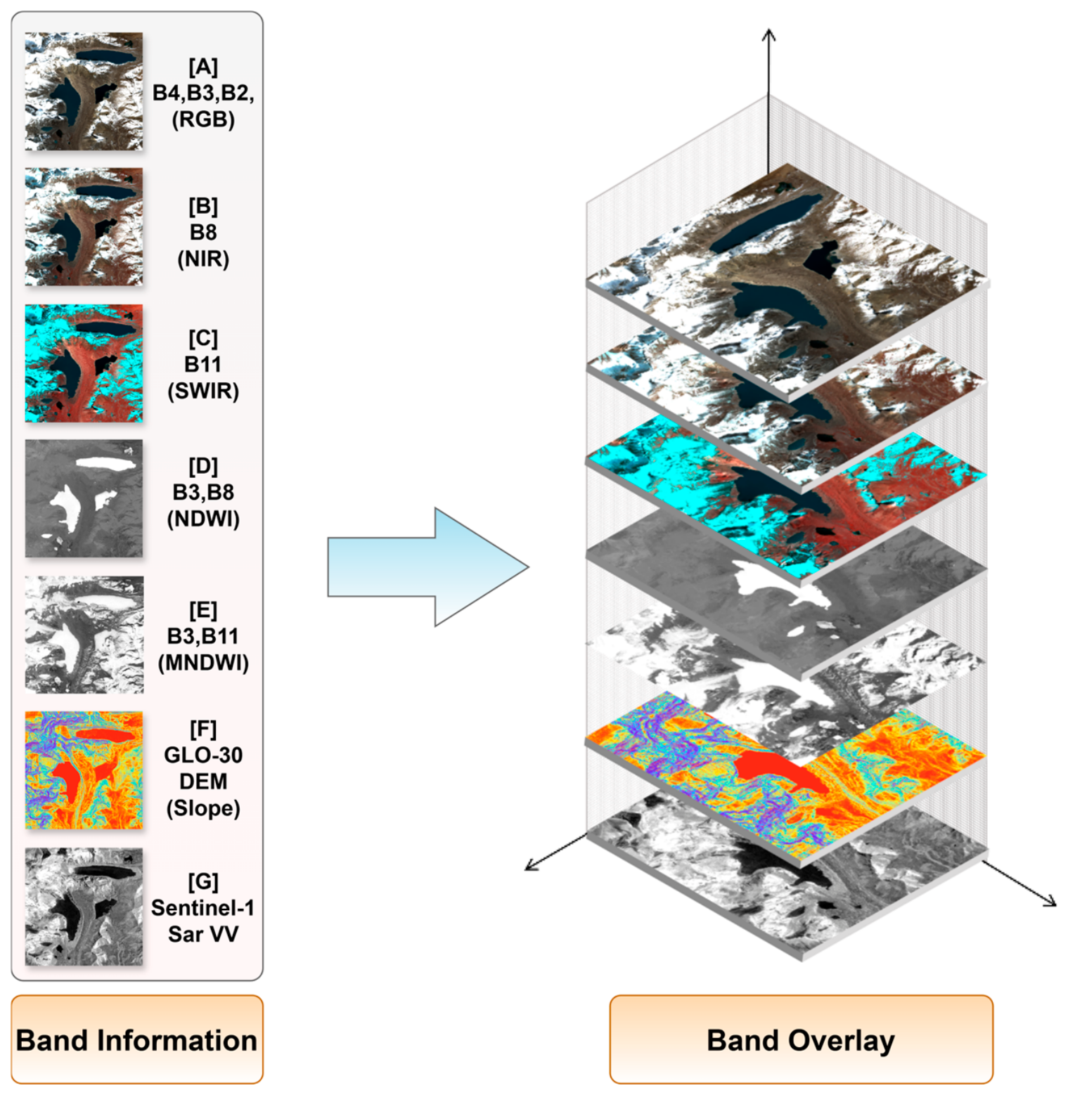
Overlay of the 9-channel multimodal remote sensing features: (A) Sentinel-2 B4/B3/B2 RGB, (B) B8 NIR, (C) B11 SWIR, (D) NDWI, (E) MNDWI, (F) slope derived from Copernicus DEM GLO-30, and (G) Sentinel-1 VV backscatter. For visualization, RGB is shown in natural color; NIR and SWIR use false-color rendering; NDWI, MNDWI, and Sentinel-1 VV are displayed in grayscale; and slope is shown using a pseudocolor gradient. Brighter tones in NDWI and MNDWI indicate stronger water-index responses.
Figure 10.
Overlay of the 9-channel multimodal remote sensing features: (A) Sentinel-2 B4/B3/B2 RGB, (B) B8 NIR, (C) B11 SWIR, (D) NDWI, (E) MNDWI, (F) slope derived from Copernicus DEM GLO-30, and (G) Sentinel-1 VV backscatter. For visualization, RGB is shown in natural color; NIR and SWIR use false-color rendering; NDWI, MNDWI, and Sentinel-1 VV are displayed in grayscale; and slope is shown using a pseudocolor gradient. Brighter tones in NDWI and MNDWI indicate stronger water-index responses.
Figure 11.
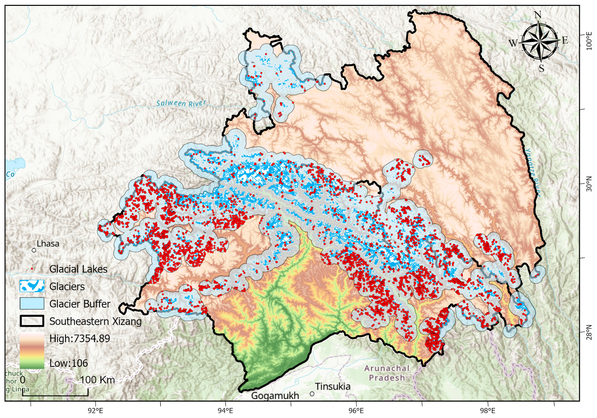
Spatial distribution of extracted glacial lakes in southeastern Tibet. (Red points indicate extracted glacial lakes, blue areas indicate glacier boundaries, and light-blue areas indicate the 10 km glacier buffer.)
Figure 11.
Spatial distribution of extracted glacial lakes in southeastern Tibet. (Red points indicate extracted glacial lakes, blue areas indicate glacier boundaries, and light-blue areas indicate the 10 km glacier buffer.)
Figure 12.
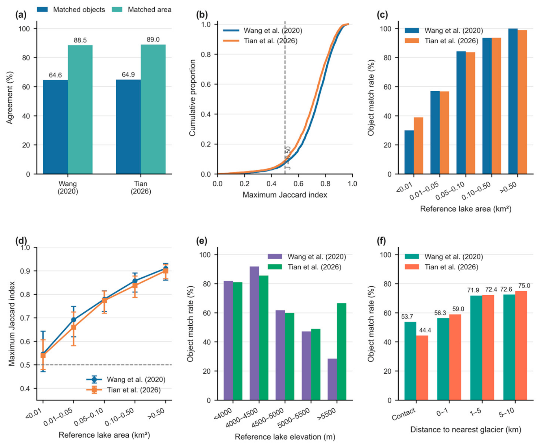
Object-level agreement between the regional glacial lake inventory produced in this study and the independent inventories of Wang et al. (2020) [
1] and Tian et al. (2026) [
11]. (
a) Overall reference-object match rate and matched reference-area proportion; (
b) empirical cumulative distribution of the maximum Jaccard index; (
c) reference-object match rate by lake-area class; (
d) median maximum Jaccard index and interquartile range by lake-area class; (
e) reference-object match rate by elevation zone; and (
f) reference-object match rate by distance to the nearest glacier. Glacier distance was calculated for both reference inventories using the same merged glacier boundaries from the Second Chinese Glacier Inventory and RGI 7.0 [
54,
55].
Figure 12.
Object-level agreement between the regional glacial lake inventory produced in this study and the independent inventories of Wang et al. (2020) [
1] and Tian et al. (2026) [
11]. (
a) Overall reference-object match rate and matched reference-area proportion; (
b) empirical cumulative distribution of the maximum Jaccard index; (
c) reference-object match rate by lake-area class; (
d) median maximum Jaccard index and interquartile range by lake-area class; (
e) reference-object match rate by elevation zone; and (
f) reference-object match rate by distance to the nearest glacier. Glacier distance was calculated for both reference inventories using the same merged glacier boundaries from the Second Chinese Glacier Inventory and RGI 7.0 [
54,
55].
Figure 13.
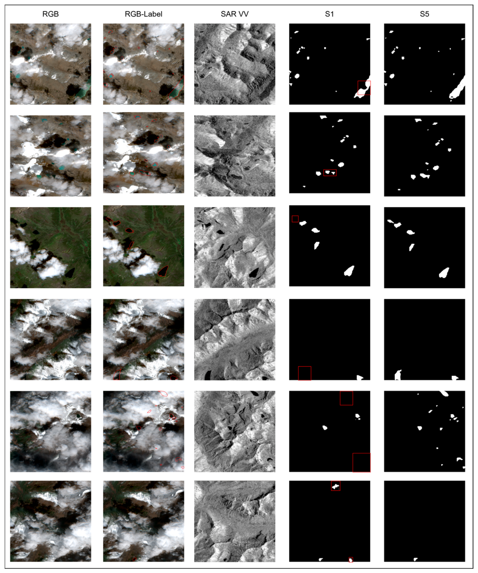
Qualitative validation of channel effectiveness in cloud- and shadow-affected scenes. From left to right: Sentinel-2 RGB; RGB overlaid with reference lake boundaries (RGB-Label); Sentinel-1 SAR (VV); the extraction result of the RGB setting (S1); and the result of the full multimodal setting (S5). Red boxes highlight representative locations where the full multimodal model (S5) improves over the RGB setting (S1).
Figure 13.
Qualitative validation of channel effectiveness in cloud- and shadow-affected scenes. From left to right: Sentinel-2 RGB; RGB overlaid with reference lake boundaries (RGB-Label); Sentinel-1 SAR (VV); the extraction result of the RGB setting (S1); and the result of the full multimodal setting (S5). Red boxes highlight representative locations where the full multimodal model (S5) improves over the RGB setting (S1).
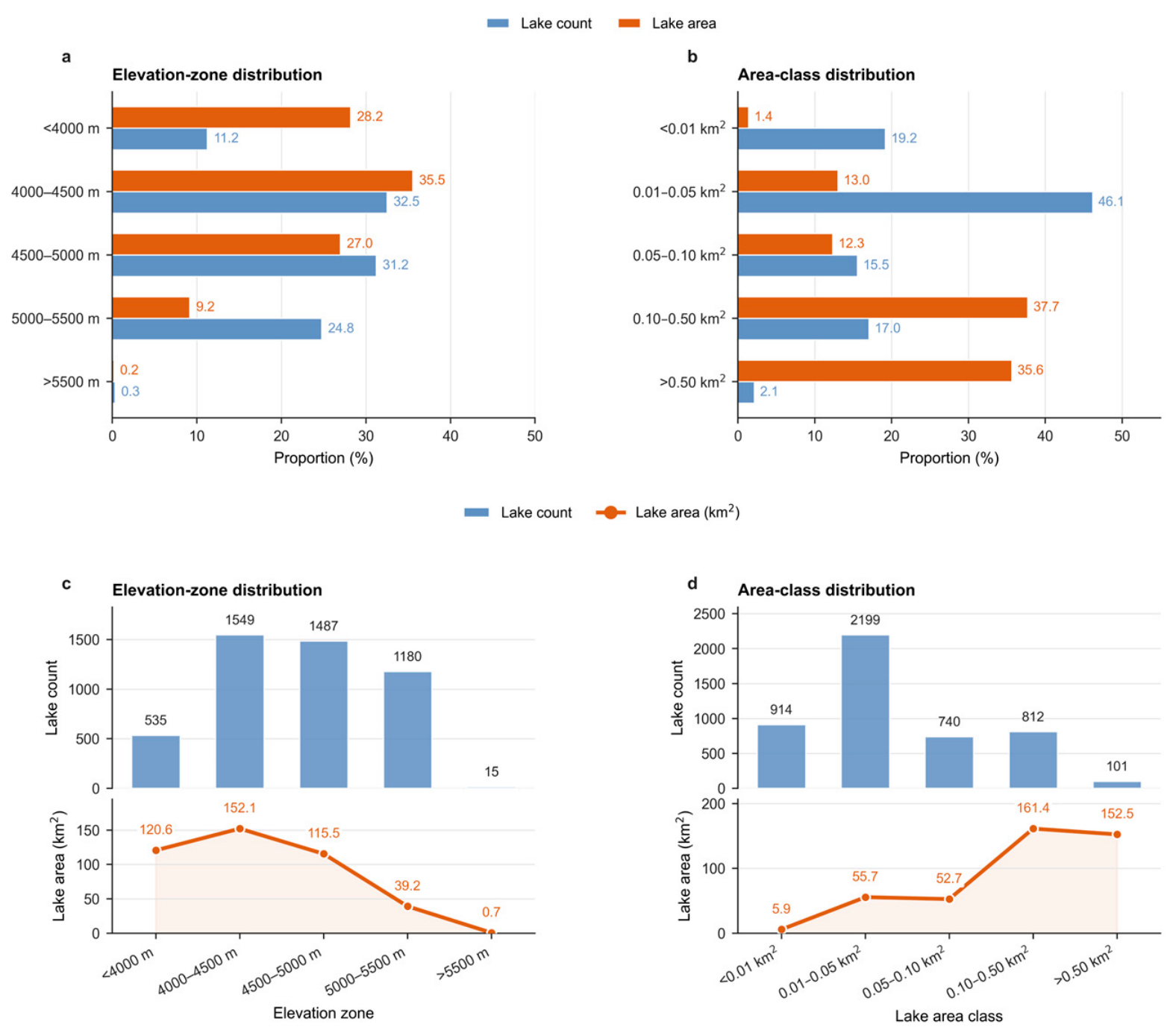
Figure 14.
Elevation-zone and area-class distribution characteristics of glacial lakes in southeastern Tibet. (a) Percentage of glacial lake number and area across elevation zones; (b) percentage of glacial lake number and area across area classes; (c) number and total area of glacial lakes across elevation zones; (d) number and total area of glacial lakes across area classes.
Figure 14.
Elevation-zone and area-class distribution characteristics of glacial lakes in southeastern Tibet. (a) Percentage of glacial lake number and area across elevation zones; (b) percentage of glacial lake number and area across area classes; (c) number and total area of glacial lakes across elevation zones; (d) number and total area of glacial lakes across area classes.
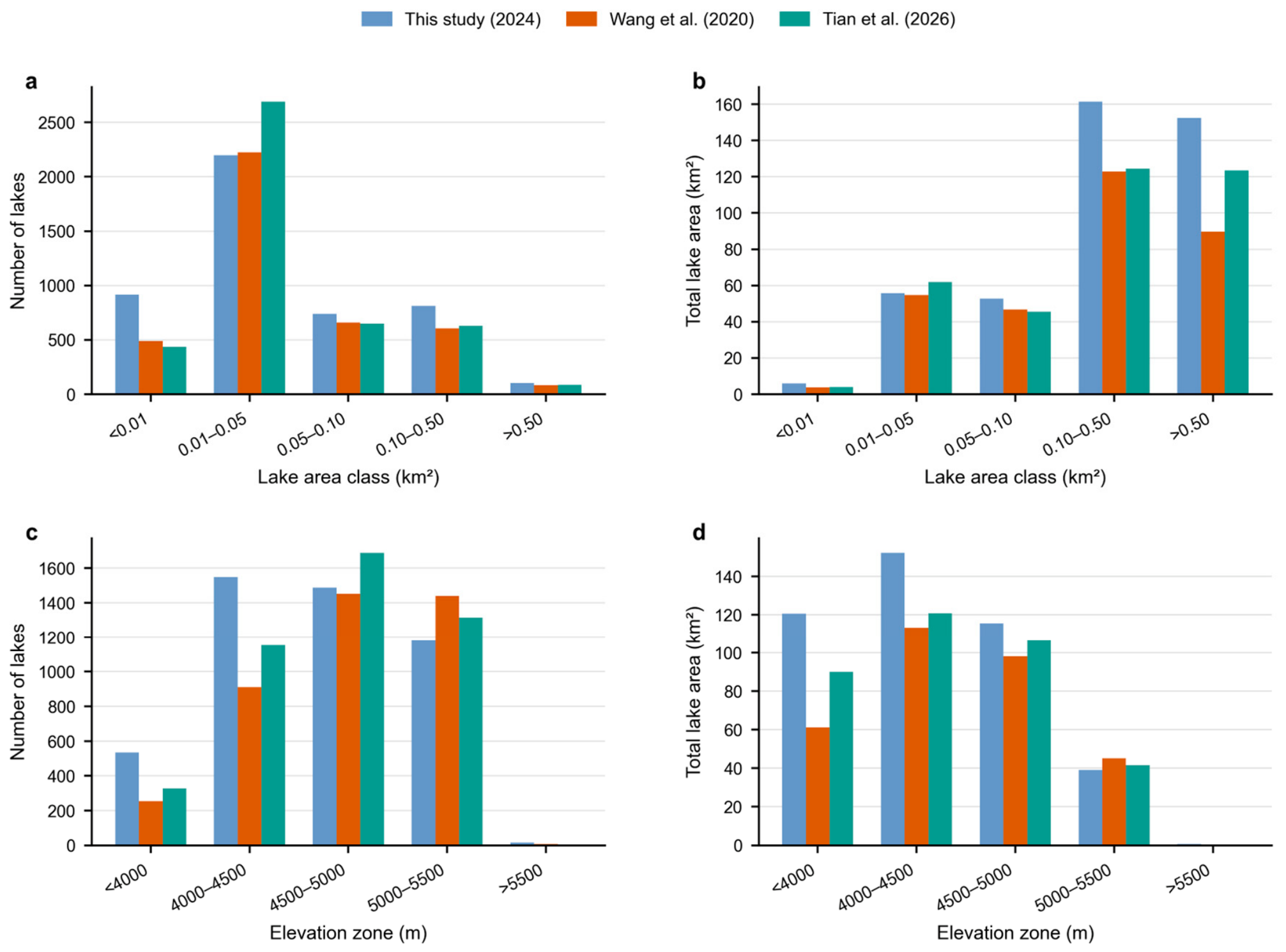
Figure 15.
Aggregate comparison of the glacial lake inventory produced in this study (2024) with the inventories of Wang et al. (2020; inventory epoch 2018) [
1] and Tian et al. (2026; inventory epoch 2023) [
11] within the study area and the common 10 km glacier-buffer extent. (
a) Number of lakes by area class; (
b) total lake area by area class; (
c) number of lakes by elevation zone; and (
d) total lake area by elevation zone.
Figure 15.
Aggregate comparison of the glacial lake inventory produced in this study (2024) with the inventories of Wang et al. (2020; inventory epoch 2018) [
1] and Tian et al. (2026; inventory epoch 2023) [
11] within the study area and the common 10 km glacier-buffer extent. (
a) Number of lakes by area class; (
b) total lake area by area class; (
c) number of lakes by elevation zone; and (
d) total lake area by elevation zone.
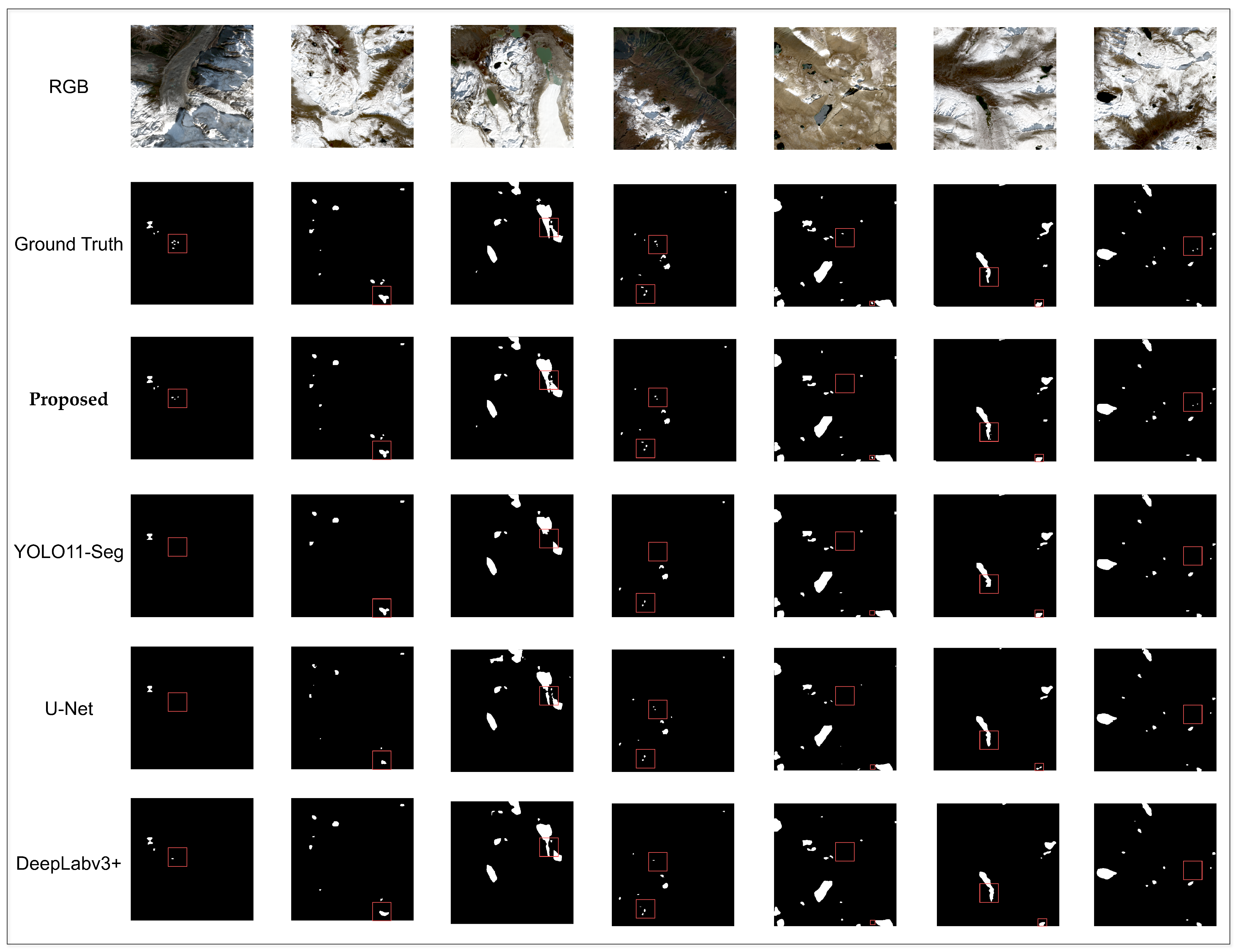
Figure 16.
Qualitative comparison across representative glacial lake scenarios, showing RGB reference imagery, ground-truth masks, and segmentation results from the proposed model, YOLO11-seg, U-Net, and DeepLabV3+. Red boxes highlight representative omissions, false detections, or boundary differences.
Figure 16.
Qualitative comparison across representative glacial lake scenarios, showing RGB reference imagery, ground-truth masks, and segmentation results from the proposed model, YOLO11-seg, U-Net, and DeepLabV3+. Red boxes highlight representative omissions, false detections, or boundary differences.
Table 1.
Main data sources used in this study. (Sentinel-2 B11 and Copernicus DEM GLO-30 were resampled and spatially aligned to a 10 m grid.)
Table 1.
Main data sources used in this study. (Sentinel-2 B11 and Copernicus DEM GLO-30 were resampled and spatially aligned to a 10 m grid.)
| Data Type | Product/Dataset ID | Spatial
Resolution | Data Source | Purpose |
|---|
| Sentinel-2 MSI | COPERNICUS/S2_SR_HARMONIZED | 10 m/20 m | Google Earth Engine Data Catalog | Optical, multispectral, and water-index features |
| Sentinel-1 SAR (VV) | COPERNICUS/S1_GRD | 10 m | SAR backscatter feature |
| Copernicus DEM GLO-30 | COPERNICUS/DEM/GLO30 | 30 m | Topographic constraint |
| Second Chinese Glacier Inventory | The Second Glacier Inventory Dataset of China, Version 1.0 | Vector data | National Tibetan Plateau Data Center | Sample checking and 10 km glacier-buffer filtering |
| Randolph Glacier Inventory | RGI 7.0/NSIDC-0770 | Vector data | NSIDC |
Table 2.
Cloud-cover thresholds, temporal windows, patch counts, and dataset split for the ten sample regions.
Table 2.
Cloud-cover thresholds, temporal windows, patch counts, and dataset split for the ten sample regions.
| Region | Stepwise Cloud-Cover Threshold Range/% | Time Window | Patches | Dataset Split |
|---|
| Region 1 | 1–5 | 1 September 2024–30 November 2024 | 1920 | Train |
| Region 2 | 0.1–0.5 | 1 January 2024–31 December 2024 | 6741 |
| Region 3 | 5–10 | 1 September 2024–30 November 2024 | 1653 |
| Region 4 | 0.1–5 | 1 May 2024–30 November 2024 | 2200 |
| Region 5 | 0.1–5 | 1 May 2024–30 November 2024 | 663 |
| Region 6 | 0.1–2 | 1 May 2024–30 November 2024 | 2223 |
| Region 7 | 0.1–2 | 1 May 2024–30 November 2024 | 798 | Val |
| Region 8 | 0.1–1 | 1 September 2024–30 November 2024 | 592 |
| Region 9 | 0.5–1 | 1 May 2024–31 December 2024 | 2479 | Test |
| Region 10 | 0.5–1.5 | 1 May 2024–30 November 2024 | 104 |
| Total | - | - | 19,373 | - |
Table 3.
Performance comparison of mainstream segmentation models.
Table 3.
Performance comparison of mainstream segmentation models.
| Model | Precision | Recall | F1-Score | mAP50(M) |
|---|
| YOLOv8-seg | 0.8803 | 0.8164 | 0.8471 | 0.8798 |
| YOLO11-seg | 0.9170 | 0.8129 | 0.8618 | 0.8898 |
| YOLO12-seg | 0.8479 | 0.8223 | 0.8349 | 0.8773 |
| YOLO26-seg | 0.8279 | 0.7977 | 0.8125 | 0.8544 |
| U-Net | 0.9498 | 0.8316 | 0.8868 | - |
| DeepLabV3+ | 0.9266 | 0.8685 | 0.8966 | - |
| Proposed | 0.9714 | 0.8746 | 0.9205 | 0.9331 |
Table 4.
Ablation experiment of the proposed modules.
Table 4.
Ablation experiment of the proposed modules.
| Setting | SPDConv | MSCA | C3k2_Mamba | C2PSA_MSCA | CARAFE | Precision | Recall | F1-Score | mAP50(M) |
|---|
| Baseline | – | – | – | – | – | 0.9170 | 0.8129 | 0.8618 | 0.8898 |
| 1 | √ | – | – | – | – | 0.9662 | 0.7196 | 0.8249 | 0.8499 |
| 2 | √ | √ | – | – | – | 0.9314 | 0.8293 | 0.8774 | 0.9045 |
| 3 | √ | √ | √ | – | – | 0.9710 | 0.8663 | 0.9157 | 0.9284 |
| 4 | √ | √ | √ | √ | – | 0.9696 | 0.8682 | 0.9161 | 0.9287 |
| 5 | √ | √ | √ | – | √ | 0.9639 | 0.8743 | 0.9170 | 0.9301 |
| 6 | √ | √ | – | √ | √ | 0.9596 | 0.8776 | 0.9167 | 0.9326 |
| 7 | √ | – | √ | √ | √ | 0.9551 | 0.8061 | 0.8743 | 0.8926 |
| 8 | – | √ | √ | √ | √ | 0.9677 | 0.8722 | 0.9175 | 0.9301 |
| 9 | √ | √ | √ | √ | √ | 0.9714 | 0.8746 | 0.9205 | 0.9331 |
Table 5.
Ablation experiment of the 9-channel input combination.
Table 5.
Ablation experiment of the 9-channel input combination.
| Setting | Input Combination | Channels | Precision | Recall | F1-Score | mAP50(M) |
|---|
| S1 | RGB | 3 | 0.9007 | 0.8509 | 0.8751 | 0.8998 |
| S2 | RGB + NIR + SWIR | 5 | 0.9146 | 0.8642 | 0.8887 | 0.9155 |
| S3 | RGB + NIR + SWIR + NDWI + MNDWI | 7 | 0.9058 | 0.8987 | 0.9022 | 0.9273 |
| S4 | RGB + NIR + SWIR + NDWI + MNDWI + Slope | 8 | 0.9040 | 0.8893 | 0.8966 | 0.9299 |
| S5 | RGB + NIR + SWIR + NDWI + MNDWI + Slope + SAR | 9 | 0.9714 | 0.8746 | 0.9205 | 0.9331 |
Table 6.
Quantitative comparison of the main models on the test set.
Table 6.
Quantitative comparison of the main models on the test set.
| Model | Precision | Recall | F1-Score | IoU |
|---|
| U-Net | 0.9294 | 0.8557 | 0.8910 | 0.8035 |
| DeepLabV3+ | 0.9264 | 0.8750 | 0.8999 | 0.8181 |
| YOLOv8-seg | 0.9436 | 0.8057 | 0.8692 | 0.7687 |
| YOLO11-seg | 0.9403 | 0.8264 | 0.8796 | 0.7851 |
| YOLO12-seg | 0.9438 | 0.7934 | 0.8621 | 0.7577 |
| YOLO26-seg | 0.9349 | 0.7788 | 0.8498 | 0.7388 |
| Proposed | 0.9135 | 0.9283 | 0.9209 | 0.8533 |
Table 7.
Elevation-zone distribution statistics of glacial lakes in southeastern Tibet.
Table 7.
Elevation-zone distribution statistics of glacial lakes in southeastern Tibet.
| Elevation Zone | Number of Glacial Lakes | Total Area/km2 | Percentage of Number/% | Percentage of Area/% |
|---|
| <4000 m | 535 | 120.6017 | 11.23 | 28.17 |
| 4000–4500 m | 1549 | 152.1352 | 32.5 | 35.54 |
| 4500–5000 m | 1487 | 115.4755 | 31.2 | 26.97 |
| 5000–5500 m | 1180 | 39.1778 | 24.76 | 9.15 |
| >5500 m | 15 | 0.7354 | 0.31 | 0.17 |
| Total | 4766 | 428.1257 | 100 | 100 |
Table 8.
Area-class distribution statistics of glacial lakes in southeastern Tibet.
Table 8.
Area-class distribution statistics of glacial lakes in southeastern Tibet.
| Area Class | Number of Glacial Lakes | Total Area/km2 | Percentage of Number/% | Percentage of Area/% |
|---|
| <0.01 km2 | 914 | 5.8643 | 19.18 | 1.37 |
| 0.01–0.05 km2 | 2199 | 55.6699 | 46.14 | 13 |
| 0.05–0.10 km2 | 740 | 52.7198 | 15.53 | 12.31 |
| 0.10–0.50 km2 | 812 | 161.3863 | 17.04 | 37.7 |
| >0.50 km2 | 101 | 152.4854 | 2.12 | 35.62 |
| Total | 4766 | 428.1257 | 100 | 100 |




 ,
,