Article

Dynamics of Forest Disturbance in the Canopy of Permanent Production Forests: A Multitemporal Analysis (2004–2025) Using Spectral Unmixing in the Southeastern Peruvian Amazon


by
Gabriel Alarcon-Aguirre
1,2,3,4,*,
Rembrandt Canahuire-Robles
1,3,
Cesar Agusto Rondan Yupanqui
3,
Mishari Rolando García Roca
1,
Liset Rodriguez Achata
3,5,
Percy A. Zevallos Pollito
1,3,
Dalmiro Ramos Enciso
3,6,
Mauro Vela-Da-Fonseca
1,3 and
Jorge Garate-Quispe
1,2,3,4
1
Departamento Académico de Ingeniería Forestal y Medio Ambiente, Facultad de Ingeniería, Universidad Nacional Amazónica de Madre de Dios, Puerto Maldonado 17001, Peru
2
Centro de Teledetección Para el Estudio y Gestión de los Recursos Naturales (CETEGERN), Facultad de Ingeniería, Universidad Nacional Amazónica de Madre de Dios, Puerto Maldonado 17001, Peru
3
Earth Sciences & Dynamics of Ecology and Landscape, Universidad Nacional Amazónica de Madre de Dios, Puerto Maldonado 17001, Peru
4
Ecology & Restoration of Tropical Ecosystems, Universidad Nacional Amazónica de Madre de Dios, Puerto Maldonado 17001, Peru
5
Departamento Académico de Ciencias Básicas, Facultad de Ingeniería, Universidad Nacional Amazónica de Madre de Dios, Puerto Maldonado 17001, Peru
6
Departamento Académico de Ingeniería de Sistemas e Informática, Facultad de Ingeniería, Universidad Nacional Amazónica de Madre de Dios, Puerto Maldonado 17001, Peru
*
Author to whom correspondence should be addressed.
Remote Sens. 2026, 18(16), 2813; https://doi.org/10.3390/rs18162813
Submission received: 30 June 2026 / Revised: 2 August 2026 / Accepted: 14 August 2026 / Published: 20 August 2026
(This article belongs to the Special Issue Forest Disturbance Monitoring with Optical Satellite Imagery)

Highlights

What are the main findings?
  • Structural degradation in the understory surpassed permanent deforestation as the primary driver of forest disturbance in the Tahuamanu Province.
  • Stratified statistical analysis revealed over 10,000 hectares of hidden forest degradation that medium-resolution optical classifications fail to detect.
What are the implications of these findings?
  • Relying exclusively on uncalibrated satellite maps underestimates actual biomass loss and conceals persistent degradation beneath a false cartographic stability.
  • Territorial monitoring and sustainable management require the mandatory statistical correction of areas and the integration of active sensors (LiDAR) to accurately monitor forest ecosystem integrity.

Abstract

Monitoring forest degradation using medium-resolution optical sensors often results in an underestimation of the actual ecological impacts, limiting conservation strategies in threatened regions. We evaluated the forest disturbance dynamics (2004–2025) in the Permanent Production Forests of Tahuamanu, Madre de Dios, Peru. We processed multitemporal Landsat images in Google Earth Engine to map change trajectories by applying Spectral Mixture Analysis to derive the Normalized Difference Fraction Index (NDFI) integrated with a stratified area estimator. This approach yielded overall accuracies of ≥93%. Our findings show that structural degradation is replacing deforestation as the main driver of forest alteration. By 2025, the footprint of this disturbance, which silently affects the understory, had quadrupled the extent of deforestation, a trend evidenced by the stratified adjustment that revealed over 10,000 hectares of structural damage previously hidden under the label of intact forest, demonstrating the typical omission bias of passive sensors. Relying on raw maps means underestimating biomass lost to understory degradation. To address this systematic bias, it is necessary to operationalize the NDFI model along with a rigorous stratified estimation. With this combined approach, a scalable, cost-effective, and statistically robust framework is offered to monitor the subtle degradation that traditional mapping systems overlook. To our knowledge, this is the first long-term, area-corrected assessment of forest disturbance within Peru’s oldest formal timber concessions, and it shows that degradation persists and accelerates even under a regulated management model.

1. Introduction

Amazonian forests play a significant role in managing the climate system of the planet by absorbing atmospheric CO2 [1]. Unfortunately, climate change, deforestation, and forest degradation are impacting this absorbing function [2]. In the region of Madre de Dios, the selective logging, the harvesting of firewood, and the grazing of cattle cause forest degradation that represents, in terms of emissions, the same level of threat as deforestation, and can surpass it [1,3,4,5,6,7]. Managing this type of forest degradation will produce climate and ecosystem benefits that will be greater and for a longer term than the simple act of planting trees [1].
Detecting these threats, however, is not straightforward. Forest monitoring efforts have traditionally relied on remote sensing approaches that have severe technical limitations when assessing complex disturbances. Most medium-resolution optical sensors and conventional vegetation indices are calibrated primarily to detect binary and abrupt changes, such as the complete loss of canopy cover associated with deforestation. However, their sensitivity decreases dramatically when attempting to capture structural alterations beneath the canopy. This physical limitation occurs because the spectral signal from the lower strata is masked by the high reflectance of the intact upper canopy, which leads to difficulties in detecting selective biomass removal or damage to the understory. Consequently, relying exclusively on assessments of the upper canopy leads to a systematic underestimation of the spatial and ecological magnitude of anthropogenic threats, in this case, forest degradation [8,9,10,11,12].
In this context, a fundamental technical and conceptual challenge arises: the difficulty of accurately identifying when and to what extent the forest is degrading. There is a distinction we must understand to address this problem. While deforestation is a drastic event in which the forest disappears completely to make way for another land use a clear change visible in any aerial photograph, forest degradation is a subtle phenomenon occurring beneath the canopy and within the forest’s internal structure. This low-intensity forest disturbance is not visible to the naked eye from a traditional satellite perspective and is often mistakenly confused with natural variations or seasonal changes [8,9,11,13]. For this reason, over the past two decades, remote sensing researchers have focused on developing tools that provide a higher level of detail to uncover what is actually happening in canopy gaps, where human activity leaves traces that conventional indices overlook [13,14,15,16].
The historical series of Landsat images has established itself as the most valuable resource for this purpose, enabling systematic observation of the Earth and the development of precise methods for quantifying forest disturbance over time [17]. However, viewing these images in the traditional way is not sufficient; a method is required that allows us to go beyond pixel color, which is where the Spectral Mixture Analysis (SMA) comes into play: a technique that assumes each pixel is a combination of pure materials called “endmembers” [9,11,18,19,20,21]. By decomposing each pixel into fractions of photosynthetic vegetation (PV), non-photosynthetic vegetation (NPV), soil, and shade, the SMA allows for the detection of disturbances associated with selective logging even when forest cover has not yet disappeared. This capacity for spectral dissection is what allows us to identify degradation trajectories ranging from undisturbed forests to overexploited areas, revealing how forest structure changes even if the forest has not yet been completely logged [20,21,22,23].
The development of indices derived from the SMA, specifically the Normalized Difference Fraction Index (NDFI), represents a qualitative leap forward in this field. The NDFI uses the sensitivity of photosynthetic capacity and the presence of exposed wood to classify areas of dense forest, degraded zones, and deforested regions [8,20,21,24,25,26,27]. Unlike traditional greenness-based vegetation indices such as the NDVI and the EVI, which track canopy cover and saturate over dense tropical forest, the NDFI is built from the soil and non-photosynthetic vegetation fractions that selective logging exposes beneath the canopy. Even indices sensitive to moisture or burn scars, such as the NBR, detect stand-replacing events more readily than the subtle sub-canopy loss of low-intensity logging. Studies in the Amazon have shown that this fraction-based formulation captures degradation that greenness-based indices tend to overlook [16,20], which is the reason we adopted it here. In many regions facing threats to forests, this need for specialized monitoring has become essential [28,29]. The implementation of this analysis on a massive regional and temporal scale is now possible thanks to the Google Earth Engine (GEE) revolution, which allows for the processing of enormous volumes of satellite data in the cloud, facilitating the creation of historical maps in less time and providing an effective tool for assessing the status of PBBs in Tahuamanu, where sustainable management depends on accurate monitoring [18,30].
Within this policy setting, Peru stands out as a highly relevant case study due to its political system and regulatory framework designed to formalize the timber sector. Specifically, the permanent production forests (BPP) of Tahuamanu Province, in the Madre de Dios region, represent much more than a land-use category; they constitute one of the most strategic and biodiverse ecosystems in the Peruvian Amazon. Their value extends beyond biological existence, as they contribute directly to human well-being and act as regulators of the carbon cycle, helping to mitigate the greenhouse gas emissions driving the global climate crisis [28,29,30,31]; despite this, this strategic importance contrasts with the reality of a territory under constant anthropogenic pressure. Tahuamanu has become an area of high anthropogenic pressure, severely impacted by logging, the expansion of shifting agriculture, and recurring forest fires. These activities have been eroding the forest’s integrity in a way that must be analyzed within the comprehensive framework of forest disturbance, a phenomenon that encompasses both the total loss of cover and the internal deterioration of the ecosystem [18,29,30,31,32,33,34]. Even though high-precision technologies, such as airborne LiDAR, can be successfully used to measure small area cover and store a lot of information with a significant level of detail, they are too expensive for repeated measurements over time and with the same frequency [35,36]. On the other hand, the dense Landsat time series will allow continued monitoring of change in forest cover over large areas that will be economically feasible [2].
The principal difficulty of Tahuamanu stems from selective logging and concomitant forest degradation which cause rapid spatiotemporal changes that can only be measured for a short period before the forest recovers. Moreover, the heterogeneity of the environment, which includes areas of living green vegetation, dead trees, and bare soil, adds another level of difficulty in accurately assessing the size of the impacted region [28,29]. It should be highlighted that Tahuamanu has the first BPP in Peru [37] which were established in December 2001 by Law No. 27308 [38] and were the first areas to develop long-term timber concessions. Because of this, the year selected for this study (2004) coincides with the logistical consolidation and the beginning of operations of the first timber concessions of that region. In the past two decades, this province has developed the largest forest sector in Peru with the largest operational and industrial scale, and highest levels of formalization and implementation of International Standards for Sustainable Forest Management [39,40]. Thus, analyzing the dynamics of Tahuamanu not only allows for the analysis of the impacts of logging under a policy framework designed to promote sustainable use, but also fills a knowledge gap. While previous studies have addressed the degradation of the Amazon rainforest on a larger scale [8,13,26], our work provides a high-density temporal analysis (21 years) on how formal timber concessions influence canopy structure in one of the most strategic and biodiverse regions of Peru.
In this context, the study evaluates the temporal dynamics of forest disturbance, defining deforestation as direct total conversion and forest degradation as structural alteration in the Tahuamanu BPP, using the SMA and the NDFI index. Specifically, we ask whether the formalized, long-established timber concession model of Tahuamanu has contained forest degradation over the past two decades, or whether structural loss has continued despite regulation. To this end, three reference years (2004, 2015 and 2025) over a 21-year period. The objective was to quantify the magnitude of the disturbance, determine annual rates of change, and classify canopy trajectories, thereby providing a methodological foundation to strengthen sustainable management policies and forest transparency mechanisms within this initial forest management framework.

2. Materials and Methods

2.1. Study Area

The study area is in Tahuamanu province, located in northeastern Madre de Dios (Figure 1). This area contains the permanent production forests of Madre de Dios, which is the second-largest forested region in the Peruvian Amazon. This area is 8568.5663 km2, containing timber concessions which border the Alto Purús National Park and buffer zone, Indigenous lands, non-timber forest concessions and cultivated lands. It is found between the parallels 10°56′23″ and 11°55′49″ south and the meridians 68°54′43″ and 70°27′54″ west (Figure 1), with an elevation of 200 to 350 m from the sea [41]. The humid tropical climate has average temperatures of 25 °C and 27 °C with short periods of cold (10 °C) from May to September [41]. There is a dry season from June to September, and a wet season from November to April [42]. This province has an average of 1740 mm of annual precipitation [41].

2.2. Method

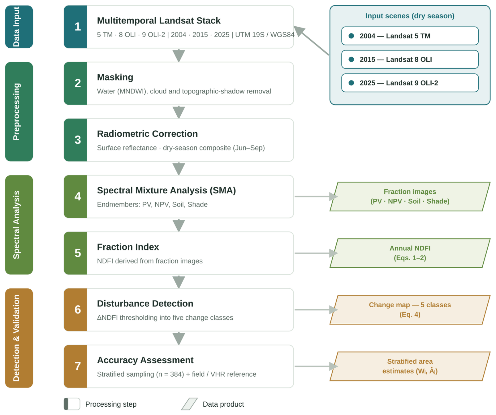
The methodological strategy is based on a multi-temporal change detection analysis designed to identify the trajectory of forest disturbance. The workflow integrates cloud-based processing (GEE, https://earthengine.google.com/, accessed on 13 August 2026), Digital Terrain Model (DTM), and sub-meter validation (Figure 2).

2.2.1. Preprocessing and Spectral Mixture Analysis (SMA)

The geospatial database was constructed using scenes from the Landsat 5 TM, 8 OLI, and 9 OLI-2 sensors (Collection 2, Level 2), georeferenced to the WRS-2 global reference system in Path/Row 002/068 and 003/068 [43]. To ensure cartographic accuracy and multitemporal comparability, all products were processed using the Universal Transverse Mercator (UTM) projection, referenced to the WGS84 datum, Zone 19 South, corresponding to the location of Tahuamanu Province.
Scenes were selected based on strict atmospheric quality criteria. Only images acquired during the dry season (June to September) and with a cloud cover percentage of less than 10% were filtered to ensure that the spectral response of the vegetation is maximized and not distorted by aerosols or persistent humidity. Following acquisition, the official radiometric scale factor was applied to convert digital elevation data to surface reflectance [17]. The imagery consists of Landsat Collection 2 Level 2 surface reflectance products. To convert these scaled integer values to physical surface reflectance, we applied the official USGS scaling factors (offset and scale). Regarding the spectral consistency between sensors, the use of Collection 2 products minimizes inter-sensor variability through standardized atmospheric correction algorithms. The transferability of the chosen endmembers across the Landsat 5, 8, and 9 platforms is supported by previous regional applications [2,34,44], which demonstrate that the NDFI index is robust to minor spectral response function variations due to the spectral unmixing of fractions rather than absolute band-wise reflectance.
Two sources of error were masked before the disturbance analysis, namely open water and topographic shadow. Water bodies were excluded with the Modified Normalized Difference Water Index (MNDWI) [45], and topographic shadows were flagged by thresholding the shade fraction retrieved from the SMA model. This distinction is reliable because deep terrain shadows and water differ spectrally. In the SMA output, shadows retain a characteristic signature, whereas water is governed by its strong absorption in the SWIR bands. The basis of the analysis consisted of applying the SMA model (Table 1), which decomposes the spectral signature of each pixel into four pure fractions or endmembers: photosynthetic vegetation (PV), non-photosynthetic vegetation (NPV) representing exposed wood and woody debris, soil, and shadow [16,21,34,46]. For each pixel and band, the observed reflectance is modeled as a linear combination of these endmember reflectances weighted by their fractions, Rβ = Σk fk·Rk,β + εβ, with the fractions constrained to be non-negative and to sum to one, and estimated by least squares. The purpose of this decomposition is to make the sub-canopy signal of degradation measurable, since selective logging exposes non-photosynthetic material and soil while the upper canopy stays partly closed, a mixture that a whole-pixel index cannot separate from intact forest. The resulting fractions of PV, NPV, soil and shade are the input to the NDFI (Equations (1) and (2)).
To ensure the comparability of the results and minimize error due to parametric variability across the years of observations (2004, 2015, and 2025), the reference reflectance values (endmembers) proposed by Souza, Roberts and Cochrane [46] were consistently used. This standardization, combined with the normalization of surface reflectance from Landsat 5 TM, 8 OLI, and 9 OLI-2, enables robust multitemporal detection of disturbance dynamics, ensuring that changes in NDFI reflect actual degradation processes rather than technical differences between satellite platforms [2,34,44].
Based on these fractions, the NDFI was calculated using Equation (1):
N D F I = G V S h a d e N P V + S o i l G V S h a d e + N P V + S o i l
where NDFI is the Normalized Difference Fraction Index, NPV is non-photosynthetic vegetation; GVshade is the fraction of vegetation normalized for shading, expressed as;
G V S h a d e = G V 1 S h a d e
The use of the NDFI to characterize degradation rests on two design choices. First, degradation is treated as a condition and disturbance as the event that produces it (Section 2.2.2), so the static NDFI describes the structural state of the forest in each year (Table 2), while the change in the index between dates (ΔNDFI) captures the disturbance events (Table 3). Second, and central to the concern about fast-growing forest, the NDFI is not a canopy-cover or greenness measure. It is derived from the sub-pixel fractions of non-photosynthetic vegetation, soil, and shade, which increase when selective logging exposes woody material and bare ground beneath a canopy that may remain closed, so the index responds to structural loss that greenness would miss even where the canopy has begun to regrow [11,20,26]. The thresholds in Table 2 were calibrated empirically for Amazonian forests rather than set arbitrarily. Because rapid canopy closure can still weaken the static signal, the disturbance classes that were validated and used for the area estimates were defined from the change between dates (ΔNDFI), a spectral-recovery class was retained to identify regenerating areas, and only dry-season composites were used, when exposed wood and soil are least masked by moisture and new foliage. Any disturbance that regrows before the following acquisition contributes to the omission that the stratified estimator corrects, so the reported areas already account for it.

2.2.2. Classification of Forest Cover

To ensure conceptual consistency, this study distinguishes between the structurally altered state of the forest and the specific physical events that cause it. In line with landscape ecology and international forest monitoring frameworks [46,47], a disturbance refers to the physical event itself, such as selective logging or the construction of infrastructure that alters the canopy over a specific period of time and is quantified using NDFI change metrics (Table 3). In contrast, forest degradation describes the loss of structural integrity or the altered condition of the ecosystem resulting from these anthropogenic impacts [48]; this persistent condition is assessed statically using NDFI thresholds (Table 2).
Forest cover for the years 2004, 2015, and 2025 was classified using static NDFI thresholds (Table 2); these cutoff values were defined based on the empirical calibration established for Amazonian forests by Souza and Roberts [20]; Souza et al. [49] and Souza, Siqueira, Sales, Fonseca, Ribeiro and Numata [8]. The categorization reflects the physical dominance of the SMA fractions: high NDFI values correspond to a closed canopy dominated by photosynthetic vegetation (PV), while a progressive decrease indicates the exposure of non-photosynthetic vegetation (NPV) and bare soil due to structural disturbances.

2.2.3. Annual Deforestation and Degradation Rate

To quantify the rate of change in permanent production forests, the annual rate-of-change formula proposed by Puyravaud [50] was applied. The use of this standardized metric (Equation (3)) has been extensively validated for monitoring forest dynamics via remote sensing in the Madre de Dios region [3,4,51,52,53]. This ensures statistical comparability between periods of different chronological durations. This provides a normalization of the rate of loss and degradation, calculated as follows:
q = 1 t 2 t 1 l n A 2 A 1 × 100
where q is the annual percentage rate, A1 and A2 are the areas of the assessed category at the beginning and end of the time period, respectively, and t2 − t1 is the elapsed time in years. This rate was calculated separately for deforestation and forest degradation across the three study periods.

2.2.4. Detection of Disturbance Dynamics

To spatially assess the magnitude of disturbances at the canopy level, a pixel-by-pixel image differentiation technique was applied to the continuous NDFI maps. This procedure generated change matrices (ΔNDFI) that quantify the loss or gain in structural integrity between the assessment periods (2015–2004 and 2025–2015) [8,16]. Spectral change was calculated using the following equation:
Δ N D F I = N D F I t 2 N D F I t 1
where ΔNDFI is the pixel’s structural change value; NDFIt2 represents the index value at the end of the evaluation period; and NDFIt1 is the value at the beginning of the period.
Subsequently, the continuous values of these difference matrices were discretized into five change categories (Table 3). The partition thresholds were first taken from the ranges reported for NDFI-based degradation mapping in the Amazon [11,20,26] and then adjusted to local conditions. We refined the boundaries by inspecting training locations on high-resolution QuickBird and WorldView imagery and on the field data, keeping the values that best isolated the spectral signal of different intensities of forest exploitation from forest stability and natural regeneration. The same thresholds were applied to the three periods so that the trajectories remain comparable.

2.2.5. Sampling Design and Validation

The accuracy of the forest cover maps and land-use transition maps was assessed using a stratified random sampling design. To determine a representative sample size that would allow for valid inferences about the entire province of Tahuamanu, the formula for infinite populations was applied. This approach was used because the study universe (pixels) is sufficiently large for the correction factor for a finite population to be statistically negligible:
n = Z 2 . p . q E 2
where the parameters are defined as follows: (1) n: Sample size (total number of inspection points); (2) Z: Critical value derived from the standard normal distribution for a 95% confidence level (Z = 1.96); (3) p: Expected probability of success, set at 50% (0.50); and (4) q: Probability of failure (1 − p = 0.50). (5) E: Maximum allowable margin of error, set at 5% (0.05).
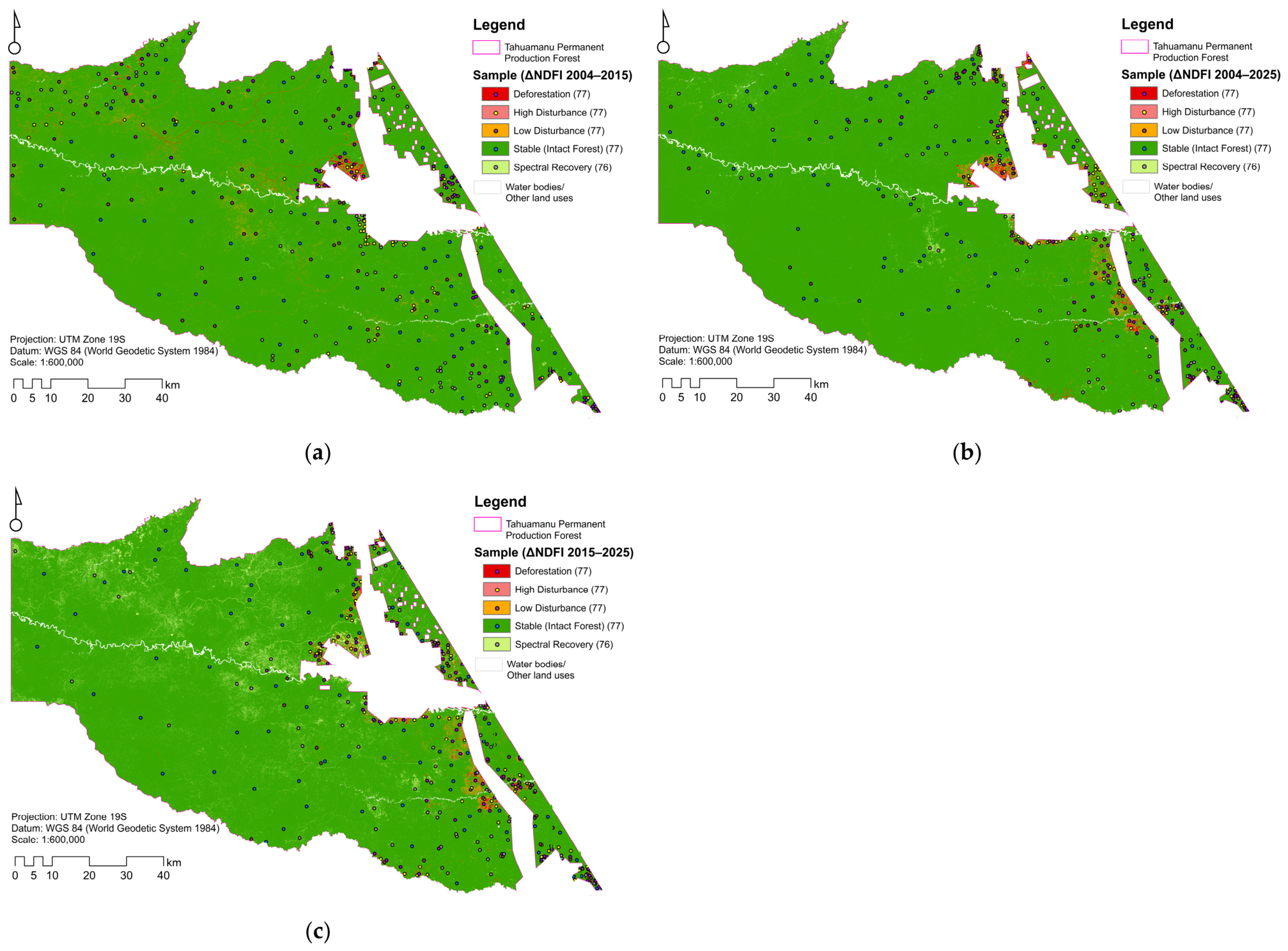
Applying these criteria, a sample size of 384 monitoring points was determined independently for each analysis period. In accordance with best practice recommendations for assessing the accuracy of changes in forest cover [54], the points were assigned using a stratified random distribution within each period. Equitable subsamples were established across the change strata to ensure the representativeness of minority classes that were ecologically important (Figure 3): stability in intact forest (77), low disturbance (77), high disturbance (77), deforestation (77), and spectral recovery (76). This equitable allocation was preferred over a proportional one because the change classes each occupy less than 2.2% of the province, whereas intact forest accounts for roughly 96% of the area (Tables S2, S5 and S8); a proportional design would therefore have assigned only two or three points to the least frequent transitions, precluding a reliable estimate of their user’s and producer’s accuracies [54,55].
The validation focused on the transition matrices for the periods of observation 2004–2015, 2015–2025, and 2004–2025. The decision to evaluate dynamic transitions (state changes) rather than individual static cover types is based on the need to capture the processes of progressive canopy degradation and recovery, an approach supported by Bullock, Woodcock and Olofsson [11] and Olofsson, Foody, Stehman and Woodcock [55] to mitigate the propagation of interannual systematic errors.
For the periods analyzed, accuracy verification was performed using a hybrid approach: (1) Historical validation (2004–2015): Given the lack of field data at the start of the study, the retrospective visual interpretation technique was employed, using very high-resolution archival images from the QuickBird (0.61 m) and WorldView (0.31–0.46 m) sensors, through visual inspection of their pan-sharpened composites available on Google Earth Pro, allowing us to confirm the presence of historical forest infrastructure at the sampled points [8]. (2) Field validation (2015–2025 and 2004–2025): Because each trajectory is expressed at the final year of the interval, and this endpoint is 2025 for both maps, the transition outcomes were confirmed with direct field data collected in Tahuamanu (GPS coordinates of clearings, logging roads and regrowth patches), which are diagnostic of the mapped change processes. This endpoint-based scheme reflects the dynamic (transition) nature of the analysis rather than a static, year-by-year verification, so the field campaign validates the 2025 state of the trajectories, not the 2004 baseline. The final quality of the classification was quantified by constructing a confusion matrix, from which metrics of overall accuracy, producer’s accuracy (PA), and user’s accuracy (UA) were derived using Equations (6)–(8) [56,57,58,59], ensuring that forest disturbance monitoring complies with international standards for cartographic accuracy.
O ^ = k n k k n
U A i = n i i n i
P A i = n j j n · j
where nkk are the correctly classified counts on the matrix diagonal, n is the total number of sample units mapped as class i (row total), nj is the total number of reference units of class j (column total), and n is the total number of validation points.
Finally, beyond the thematic evaluation, these confusion matrices (Tables S1–S9) were used as the mathematical basis for implementing the stratified area estimator. To ensure the reproducibility of the statistical fit, the procedure was structured by integrating the validation counts with the mapped area; first, the weight of each spatial stratum (Wi) was calculated by dividing the mapped area of each class by the total area of the evaluated forest. Subsequently, the sample counts from the matrix were converted into a matrix of estimated area proportions ( p ^ i j ), weighting agreement and classification errors by the spatial weight of their respective cartographic stratum (Wi).
p ^ i j = W i n i j n i
where nij is the number of sample units of map class i assigned to reference class j, and n is the total number of sample units in map class i.
The sum of these weighted proportions allowed for the calculation of the adjusted area estimate (Âj) for each trajectory, directly compensating for the directional bias of the optical sensor’s omissions and commissions.
 j = A t o t a l i p ^ i j
where Atotal is the total mapped area of the evaluated forest.
A worked example of this weighting is given in Tables S3, S6 and S9. Because each stratum re-enters the calculation through its true area weight (Wi), the estimator remains design-unbiased under any allocation, so the more intensive sampling of the minority change classes does not inflate their estimated areas and affects only the variance of the estimates, not their expected value. The uncertainty of these estimates was quantified through the standard error of the stratified estimate, which provided the variance needed to report the adjusted areas of deforestation and structural degradation with 95% confidence intervals.
S ( p ^ j ) = i W i 2 n i j / n i 1 n i j / n i n i 1
S A ^ j = A t o t a l   S p ^ j ,   C I 95 % = A ^ j ± 1.96   S A ^ j
where S( p ^ j ) is the standard error of the estimated area proportion of class j, and S(Âj) is the standard error of the adjusted area, from which the 95% confidence interval is obtained.
The equitable allocation was chosen to obtain reliable class-level accuracy for the minority change classes rather than to minimize the variance of their area estimates. Because the area of a rare class depends largely on omission errors within the dominant stable stratum, its adjusted area still carries a wide confidence interval, whereas the stable-forest and deforestation areas are estimated precisely (Table S7) [55].

3. Results

3.1. Validation

The accuracy assessment confirmed the reliability of the NDFI-based model for detecting forest change trajectories (Table 4) and the findings indicate that the NDFI model produced consistent overall accuracy figures over the various time periods. For 2004–2015, accuracy was 93.2%, and 2015–2025 = 93.5%. For the total historical period, accuracy was 93.0%.
High classification performance was similarly achieved for specific landscape categories. The intact forest was almost perfect with UA and PA of 98.7% with omission and commission errors of only 1.3%. Likewise, deforestation maintained accuracy above 96.1%. The results confirmed the robust deforestation canopy loss threshold. Spectral recover class also showed good separability with values in the range of 93.4% to 94.7% for the period of analysis with stable metrics.
As is typical in remote sensing of Amazonian forests, the degradation classes exhibited the highest margins of error due to the complexity of the spectral mix, though accuracy was still high. The low disturbance class had the lowest accuracy values in the matrix (87.0–88.3%), resulting in omission and commission errors of up to 13.0%. The complete error breakdown by class and period is provided in the Supplementary Material (Tables S1–S9).

3.2. Classification of Forest Cover

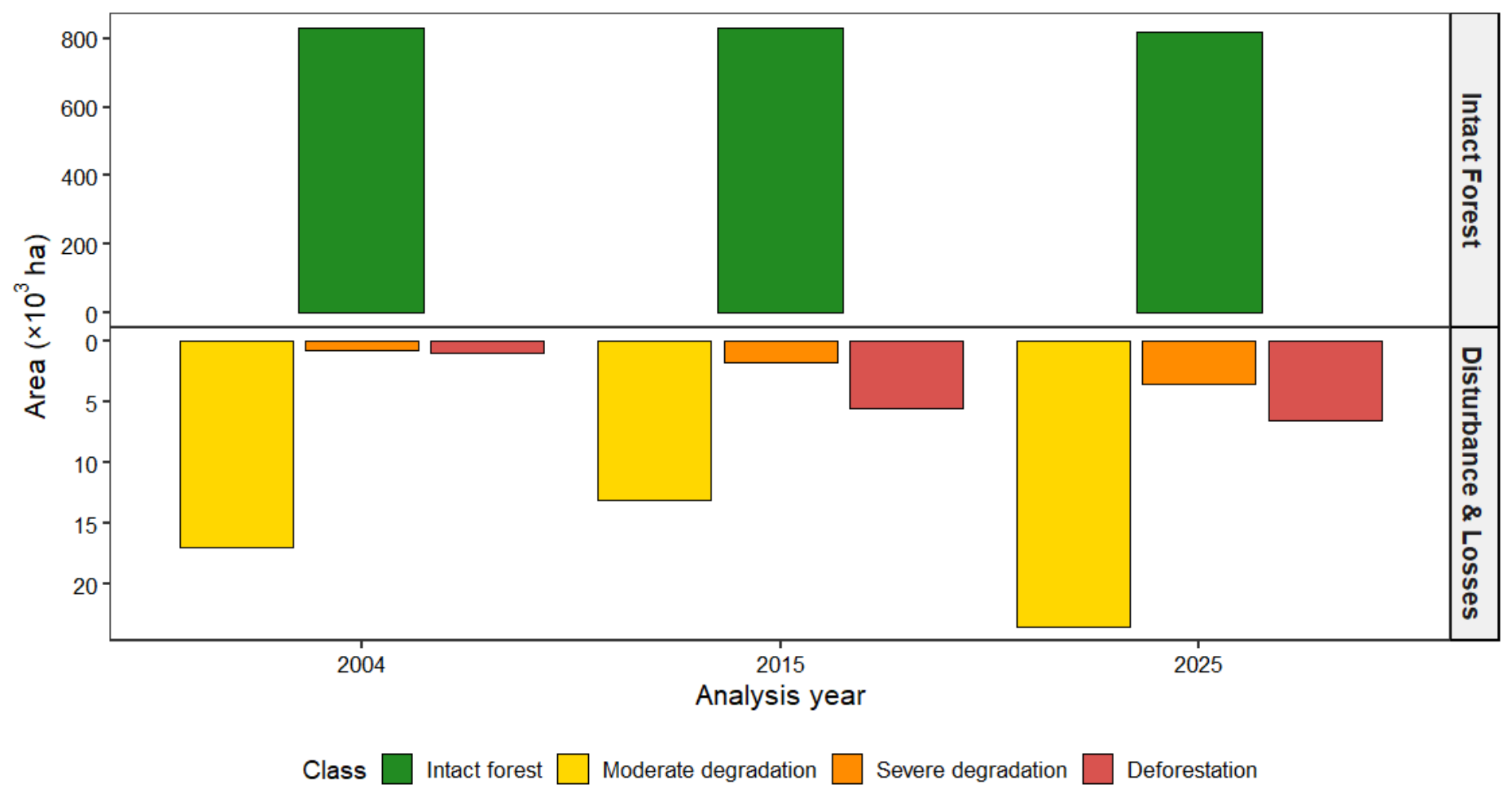
The categorization of forest integrity across the 84,983.8 ha of the Tahuamanu study area indicates a landscape that has historically been dominated by structurally undisturbed canopy, but is now undergoing progressive structural deterioration (Table 5). For the period of analysis, intact forest was the primary land cover, and recorded a gradual decrease due to deforestation from 831,188 ha in 2004 to 816,269 ha in 2025, a reduction of 14,919 ha. Deterioration of intact forest throughout this period indicates the conversion of stable forest to multiple forms of disturbed forest.
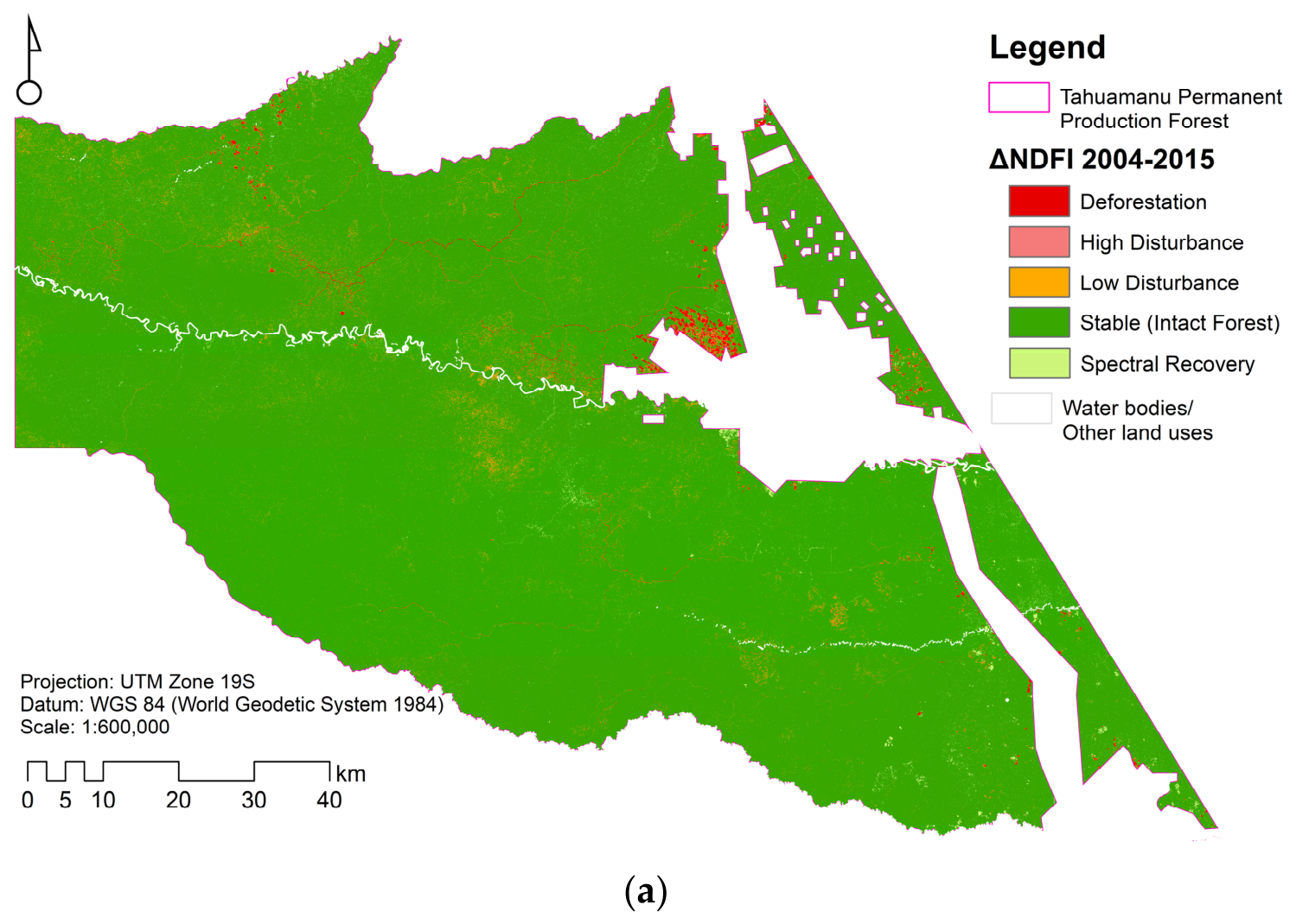
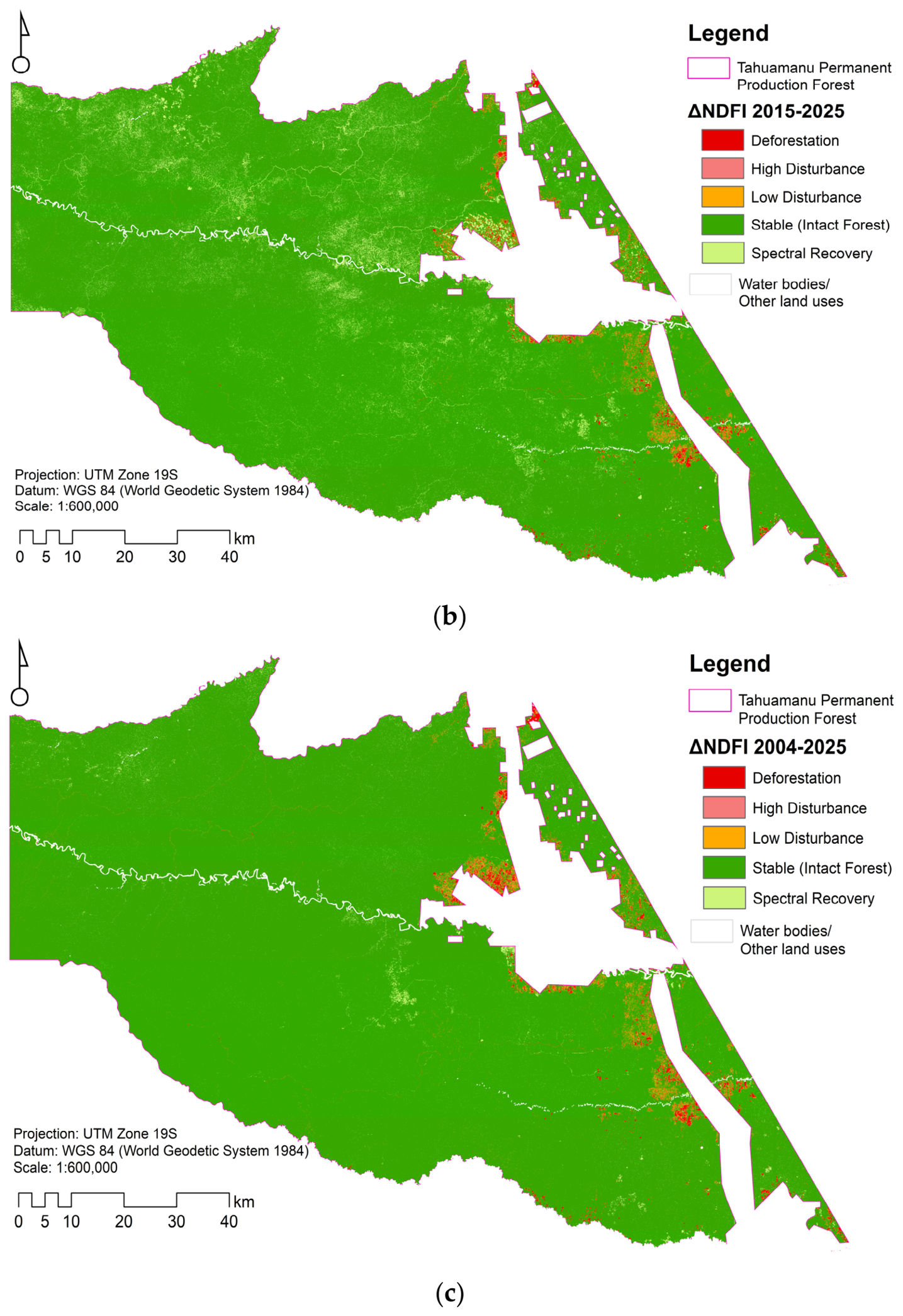
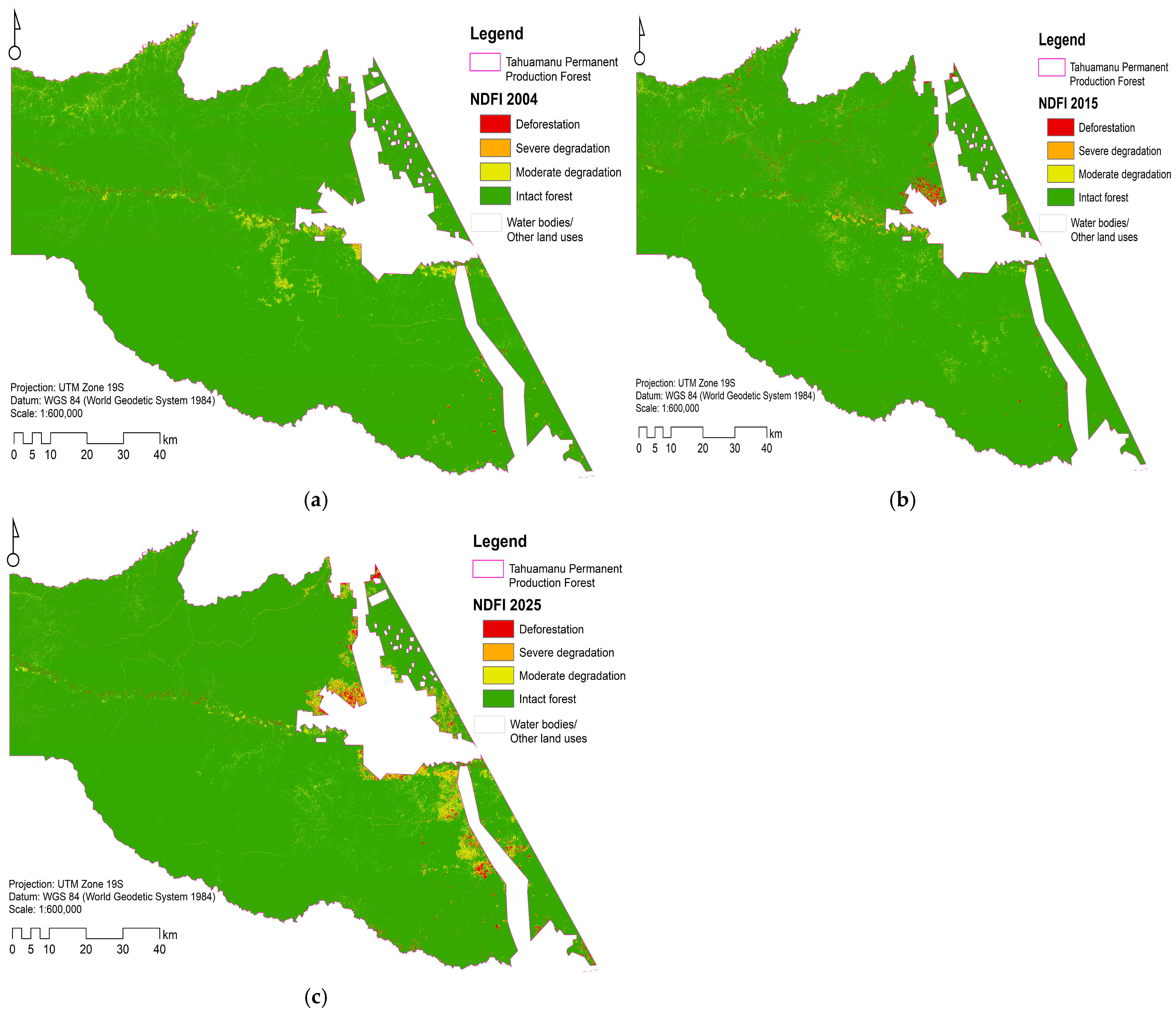
Deforestation exhibited continuous, non-linear growth. In 2004, deforestation was minimal, covering 995 ha (0.1%); however, the area increased 5 times to 5506 ha in 2015, and deforested area continued to grow to 6567 ha (0.8%) in 2025, an increase of 1061 ha deforested. The deforestation patterns displayed in the spatial maps (Figure 4) show the evolution from dispersed clear-cut areas to merged zones of deforestation.
In contrast, canopy degradation demonstrated inconsistent patterns. During the first period, the total degraded area decreased from 17,655 ha (2.1%) in 2004 to 14,792 ha (1.7%) in 2015. This decline was largely a result of the decrease in moderately degraded areas. However, during the subsequent period from 2015 to 2025, there was a considerable rise in forest degradation, reaching 27,002 ha (3.2%), a rise of 12,210 ha degraded. This indicates that during 2015–2025, more extensive disturbance was caused to the canopy compared to deforestation.
For both of the periods observed, moderate degradation was the principal disturbance category, rising from 16,907 ha in 2004 to 23,496 ha in 2025 and increase of 6589 ha. That exceeded the extent of severe degradation, though severe canopy disturbance also grew, expanding from 748 ha in 2004 to 3505 ha in 2025. The micro- and macro-disturbances in the scaled panels (Figure 4 and Figure 5) provide a visual estimation to support these area assessments, demonstrating how moderate and severe degradation encroached upon the permanent production forest.

3.3. Annual Rate of Deforestation and Forest Degradation

Analysis of the change metrics (Table 6) reveals a marked acceleration in the loss of intact forest over the past decade; between 2004 and 2015, the area of intact forest declined at a conservative rate of 150 ha·year−1 (−0.02%). However, during the 2015–2025 period, this rate of decline increased nearly ninefold, reaching 1327 ha·year−1 (−0.16%), resulting in a much higher negative rate of −0.09% in change in forest cover.
The first decade (2004–2015) registered the most aggressive deforestation with deforestation dynamics showing a time-reverse pattern with a first accelerating and a subsequently decelerating phase, showing a rate of deforestation of 16.83% (410 ha·year−1) per year, corresponding to a total of 4511 ha of cut down forest area in that period. After that, in the second decade (2015–2025), deforestation pressure decreased by 1.78% (106 ha·year−1). Despite the deceleration, the historical deforestation pressure of the province shows a sustained pressure of 9.40% corresponding to a total of 5573 ha of deforestation in the province.
Canopy degradation trends display distinct patterns based on intensity levels. For severe degradation, the trends were characterized by sustained rapid growth, with annual expansion rates of 7.87% and 7.36% per year for the first and second periods (each representing 2757 ha), respectively. The situation for moderate degradation was different, where a contraction occurred during the 2004–2015 period (with a rate of −2.31%), followed by expansion. The 2015–2025 period exhibited a positive change of an additional 10,426 hectares of moderate degradation, at a rate of 6.04% per year. This situation indicates that, in the recent past, the activity regarding changes in the Tahuamanu landscape shifted from deforestation toward more extensive partial canopy degradation.

3.4. Disturbance Dynamics and Area Adjustment

The stratified area estimates (Table 7) reveal discrepancies between the areas mapped using pixel counting and the final estimates adjusted for classification errors. Throughout the evaluated timeline, the spatial model systematically underestimated forest degradation. In the complete historical assessment (2004–2025), the original map overestimated the extent of the intact forest by more than 10,000 hectares (814,873 ha mapped versus 804,569 ha adjusted).
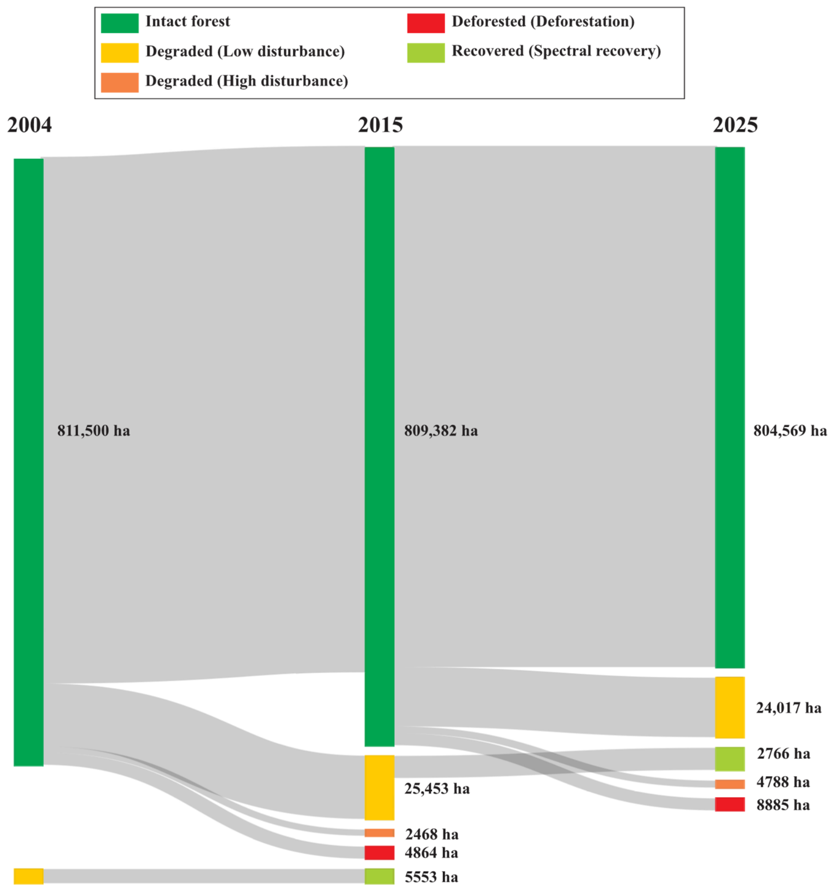
The impact of this satellite bias varies by decade. The largest detection gap appeared in the first period (2004–2015). While the spatial analysis reported 17,940 ha of total disturbance, the stratified adjustment revealed much more degradation, 27,921 ha. Low disturbance was primarily responsible for this omission, rising from 16,327 ha mapped to 25,453 ha adjusted (Table S10).
This underestimation persisted into the following decade (2015–2025), though with a different composition in terms of severity. The map identified 16,422 ha of total disturbance, which the stratified calculation corrected to 26,783 ha. In this recent period, high disturbance began to account for a larger share of the adjusted estimates, at 2766 ha against the 1818 ha mapped.
In contrast to the underestimated degradation, the canopy-loss trajectories kept high spectral fidelity, with deforestation showing only minimal pixel overestimation across all intervals. For 2004–2025, its adjusted area came to 6015 ha, close to the 6237 ha of the raw map. Spectral recovery went the other way, underestimated by the satellite in every period and reaching an adjusted 8461 ha over the full record. Figure 6 and Figure 7 show the spatial distribution of these transitions.

4. Discussion

4.1. Spatial Patterns: Driving Forces of Alteration in Tahuamanu

Quantification of forest integrity categories reveals that the structural degradation is driven by spatially and temporally distinct forces. In Tahuamanu Province, Madre de Dios, Peru, one key finding is the absolute predominance of subtle degradation over definitive loss of cover. This pattern is consistent with broader regional dynamics, where the spatial impact of degradation exceeds that of deforestation [13,60]. By 2025, total degradation (27,002 ha) quadrupled the extent of deforestation (6567 ha). This disproportion empirically corroborates questions regarding the viability and sustainability of the current timber harvesting model in Peru’s natural forests [39,40]. In turn, this finding demonstrates that the primary threat to this forest ecosystem does not lie in its conversion, but rather in the progressive deterioration of its internal architecture [34]. The net transition of nearly 15,000 hectares of intact canopy to various states of disturbance reveals a subtle yet extensive alteration that compromises long-term forest cover, revealing a significant unrecognized vulnerability in the Madre de Dios region [1].
An analysis of the spatial distribution of these processes (Figure 3), seen within the land-use dynamics in the southwestern Amazon [3,9], shows that forest loss and degradation follow different causes. Deforestation forms dense, consolidated patches, and in the Tahuamanu production forests it follows two patterns. Along the boundary it reflects pressure from the agricultural frontier and shifting cultivation that advance into the margins [3,51]. Inside the concessions, a second component tracks the logging infrastructure and concentrates around timber collection yards and established primary roads. Forest degradation, by contrast, penetrates the interior of the continuous forest, linked to the operational framework of the forest concession contracts and the overlapping harvesting of non-timber forest products [4,39].
The temporal dynamics of the forest disturbance categories confirm the direct and persistent impact of forest management on the ground. The decline in moderate degradation observed in 2015 reflects the cyclical nature of concessions, indicating likely periods of inactivity or rest in logged plots that allowed for the incipient spectral closure of the upper canopy. However, this apparent resilience is reversed by the alarming resurgence recorded in the last decade (2015–2025), during which disturbance events aggressively invaded new concession areas (Figure 4). The expansive construction of forest road networks and the expansion of selective logging together systematically fragment the understory microclimate [13,33]. On the other hand, the uninterrupted growth of severe degradation (3505 ha) is concerning, an indicator that recent extractive regimes are overwhelming the ecosystem’s natural recovery capacity and pushing forest integrity toward critical alteration thresholds. A formal attribution that integrates road-expansion time series, per-concession harvest records and settlement growth was beyond the scope of this study and is limited by the availability of these layers for the full period. It remains a useful next step for disentangling the relative weight of each driver.

4.2. Temporal Acceleration and the Shift Toward Degradation

An analysis of annual rates of change reveals a concerning ecological transition in the province. The pressure on the ecosystem has not decreased, but rather has changed in the way it manifests itself. During the first decade (2004–2015), production forests bore the brunt of deforestation (reaching 410 ha·year−1). This initial trajectory of cover loss coincides with the early phases of agricultural frontier expansion and the expansive development of road infrastructure in the Madre de Dios region [1,4,5,7,30,61]. However, the marked slowdown in deforestation recorded in the most recent decade (2015–2025) is a false indicator of territorial stability.
Far from a recovery or a scenario of effective conservation, the most recent period saw an acceleration in the loss of intact forest (1327 ha·year−1), driven by an explosive increase in disturbances at the subpixel scale [1,60]. The trajectory of moderate degradation, which initially showed a decline, was drastically reversed, adding more than 10,000 new hectares to the area with structural damage. This expansion, coupled with the sustained advance of severe degradation, demonstrates an undeniable shift in the threats to forest integrity [13,34].
This shift in disturbance dynamics underscores that biomass loss in Tahuamanu no longer occurs primarily through clear-cutting for agriculture, but rather through structural degradation associated with the intensification of logging activities within concession areas [4,39]. The high rates of recent disturbance indicate that current harvesting regimes, far from ensuring sustainable forest use [40], are straining the ecosystem’s resilience and pushing production forest cover toward a state of persistent degradation [13,34]. Unlike large-scale regional studies that treat forest degradation as a widespread and often unregulated phenomenon, our 21-year analysis of Tahuamanu offers a new perspective: the ability to assess degradation trajectories within a formalized forest management framework. Whereas the existing Amazonian literature has extensively documented that degradation exceeds deforestation in terms of affected area [13,34], our study goes further by revealing that forest degradation does not cease even under regulated and standardized timber concession schemes. This finding constitutes an original scientific contribution, as it demonstrates that the invisible footprint of selective logging, characterized by understory fragmentation and the proliferation of secondary roads, persists and indeed accelerates regardless of the legal formality of the concessions. Consequently, the novelty of this study lies in challenging the assumed effectiveness of current regulatory frameworks in curbing forest degradation, providing long-term empirical evidence of the divergence between the theoretical sustainability of the concession model and the ecological reality of canopy integrity.

4.3. Spectral Limitations and Understory Disturbance Detection

The assessment of mapping accuracy confirms the validity of the NDFI in identifying signs of forest disturbance, achieving consistently high overall accuracies (≥93.0%) across all time periods. However, the true value of this validation lies not in the high performance of categories such as intact forest or deforestation, whose accuracies exceeded 96%, but in the spectral behavior of the disturbance classes. The fact that low disturbance recorded the highest error margins in the matrix (up to 13.0%) does not constitute an algorithmic deficiency in the classification, but rather an empirical manifestation of the physical limitations inherent to medium-resolution optical sensors when faced with the complexity of the Amazonian ecosystem [8,11,20,21,62].
In the logging areas of Tahuamanu, degradation occurs covertly, where low-intensity selective logging fragments the understory but keeps the upper tree canopy partially closed. This three-dimensional architectural reconfiguration masks the loss of understory biomass, diluting the disturbance signal within the reflectance of a 30 m resolution pixel [13,63,64]. Under these complex conditions of spectral mixing in ecological transition zones, disturbance discrimination was still around 87.0%. This may be near the upper limit of effectiveness that passive optical remote sensing can offer for detecting subtle degradation [11,65].
Far from limiting the study’s reliability, the quantification of these spatial confusion margins plays an important role in improving the estimation of forest degradation. In accordance with established guidelines for assessing land-cover changes [54,55], these errors serve as the mathematical input for the stratified estimator. By explicitly mapping where and how the satellite confuses subpixel-scale degradation with intact forest, the biased paradigm of direct pixel counting is abandoned, allowing the error matrix to act as the statistical calibration vector necessary to calculate areas adjusted with probabilistic rigor.
The use of fixed NDFI thresholds across the 2004–2025 period raises a valid concern about inter-sensor variability between Landsat 5 TM and Landsat 8/9 OLI. We consider our classification adequate to address it on physical grounds. Because NDFI is computed from fractional abundances (PV, NPV, Soil) rather than from absolute top-of-atmosphere reflectance, it remains largely insensitive to the spectral response functions of each sensor [2,34]. This is reinforced by our use of Landsat Collection 2 Level 2 products, which apply the same atmospheric-correction routines to every platform and keep the time series consistent [43]. Restricting the analysis to the dry season and fixing the endmembers to established Amazonian spectral profiles further limits phenological noise and atmospheric variability [8,46]. For these reasons, the shifts we observe in forest integrity are best read as genuine changes in canopy structure rather than artifacts of the sensor transition or classification inconsistency [44].

4.4. Adjusted Areas, Subtle Degradation, and Future Perspectives

Statistical correction of the mapped areas reveals a more severe territorial reality than that captured by a simple pixel count, demonstrating that the apparent stability of the canopy in Tahuamanu is, to a large extent, a biased spatial representation. The fact that the stratified estimator reclassified more than 10,000 hectares from the historical inventory of Intact Forest to degraded forest classes empirically confirms the omission bias that medium-resolution optical sensors exhibit [11,54]. The significant extent of concealed structural damage underscores the danger of assessing the condition of Amazonian forests based solely on raw maps, which underestimate the fragmentation of the understory.
When this trend was broken down over time, the adjusted figures revealed a troubling shift in the impact of logging practices. The significant detection gap in the first decade where approximately 9100 ha of low disturbance was invisible to the spatial classifier, reflecting low-intensity selective logging, typical of the initial stages of operations in timber and non-timber (Brazil nut) concessions [4,33]. However, the persistence of this underestimation during the recent period (2015–2025), coupled with the proportional increase in adjusted high disturbance (2766), signals an intensification of logging operations. The increase in degraded forest area suggests a more aggressive expansion of the network of secondary roads within the production forests, and the rise in severely degraded forests indicates an increase in harvesting density per hectare [4,13].
This dichotomy in spatial detection where deforestation exhibits nearly perfect spectral fidelity due to homogeneous surfaces, while degradation acts as an extensive and diffuse matrix that penetrates the continuous canopy [13,20] redefines the challenges of environmental monitoring in the Amazon and other threatened forest regions [4,11]. The fitted trajectories show that the alteration of forests is not dominated by clearing, but rather by structural degradation [4,11]. In terms of future prospects, the magnitude of these underestimated areas underscores the urgent need to broaden the territorial monitoring paradigm in the Amazon and other threatened forest regions. While future research may consider integrating active detection technologies (LiDAR) or high-spatial-resolution optical constellations [9,66], the priority for forest management should be the operationalization of the approach presented. Emphasizing the NDFI model developed with a stratified area estimate provides a scalable, economically viable, and statistically robust framework for monitoring the extent of subtle forest degradation that conventional maps systematically overlook [12,62,67].

4.5. Comparison with Other Amazonian Forest Studies

Situating these results within the wider Amazonian literature supports their generalizability. The predominance of degradation over outright forest loss that we observe in Tahuamanu matches the pattern reported at regional and basin-wide scales, where degraded area exceeds deforested area and carries a comparable or greater climatic cost [13,26,34]. Studies in the southwestern Amazon have likewise attributed forest disturbance to road expansion and selective logging [4,6,33], the same drivers we identify inside the concession system, which suggests that the process we document is a local expression of a common regional dynamic rather than an isolated case.
The methods also agree. Our workflow, built on SMA, NDFI and a stratified area estimator, belongs to the same family of Landsat-based approaches applied across the Brazilian Amazon [11,16,46], and our overall accuracies (≥93%) fall within the range reported by those studies [8,11]. This agreement suggests that the method performs within the usual range for the biome and that the Tahuamanu estimates can be compared directly with results obtained elsewhere. At the same time, the 21-year span covered here, assessed across three periods, adds temporal depth that many regional snapshots lack, which supports the transferability of the conclusions to other managed forests of the region.

4.6. Sources of Uncertainty and Data Limitations

Several sources of uncertainty beyond the spectral mixing should be considered when interpreting these results. The transition between sensors is the first. As noted in Section 4.3, the use of Collection 2 Level 2 products and the fraction-based formulation of NDFI limit the influence of the different spectral response functions of Landsat 5 TM, 8 OLI and 9 OLI-2 [25,43,46], although residual cross-sensor differences cannot be ruled out entirely.
Atmospheric conditions are a second source of error. Persistent cloud cover in the humid tropics reduces the number of clear observations and can leave contaminated pixels in annual composites [2]. We restricted the analysis to the dry season and applied cloud and shadow masking, which lowers this risk, although some residual haze or thin cloud may remain. Topographic shadowing is a related concern, since deep shadows can be confused with water or with other low-reflectance surfaces. We addressed it by thresholding the shade fraction from the SMA model and by masking water with the MNDWI [45], yet in the more dissected terrain a small amount of shadow-induced confusion may persist. Two further factors relate to the spectral method itself. The choice of SMA endmembers can shift the fraction values and therefore the NDFI, so we used a fixed set of endmembers drawn from established Amazonian spectral profiles and applied it to every date, which keeps the decomposition consistent through time [19,46]. Seasonal variation is limited by restricting the analysis to dry-season composites, so phenological differences between dates are small [1]. Terrain-induced shadow is a minor factor here because the study area is a lowland landscape of gentle relief, and any small residual is removed by the shade-fraction mask described above.
Finally, the spatial resolution of Landsat sets a physical limit on what can be detected. Degradation that occurs below the 30 m pixel, particularly very low-intensity selective logging under a closed canopy, is only partially captured, which is the main reason the low disturbance class carries the largest error and why the stratified adjustment increases its area. Gaps in the historical Landsat archive and geolocation differences between dates are additional, if minor, contributors. The disturbance classes rely on a single set of ΔNDFI thresholds applied across the province. Although the study area is a fairly homogeneous forest type, some threshold-related uncertainty remains, and it is captured by the accuracy assessment and corrected through the stratified estimator. None of these limitations bias the adjusted areas, because the stratified estimator corrects for classification error, but they set the boundaries within which the results should be read and point to the value of complementary data such as high-resolution optical imagery or LiDAR in future work [35,36,66].

4.7. Selection of the NDFI Among Current Forest Disturbance-Monitoring Methods

Forest disturbance monitoring now spans several families of methods, and it is worth explaining why we used the NDFI. One family relies on dense time series of every available Landsat observation to detect breakpoints, including trajectory-based and continuous change detection algorithms and the continuous degradation methods built on spectral unmixing [10,11]. These methods identify when a change occurred and separate gradual degradation from forest loss, but they need many observations per year. In the southwestern Amazon, where cloud cover limits the usable Landsat record [2], that condition is hard to meet across two decades, and the earliest years around 2004 are especially sparse.
A second family works from spectral decomposition, using the fractions of photosynthetic vegetation, non-photosynthetic vegetation, soil and shade to build indicators such as the NDFI or tools like CLASlite [11,16,18,19]. These methods do not need a continuous record. They can be applied to a few dry-season composites, and the NDFI has a physical meaning because it responds to the non-photosynthetic material and soil that selective logging exposes beneath the canopy. For a study based on three reference points (2004, 2015 and 2025) in a cloudy region, this per-date approach fits the data better than a dense time-series algorithm and can be reproduced at provincial scale in GEE.
We used the NDFI because it fits the data and the question, not because it is the only option. It detects sub-canopy degradation, works with a sparse observation record, and can be applied elsewhere. We did not run a side-by-side comparison with time-series algorithms, which would need a denser Landsat stack than is available for the full period, and we leave this for future work. Annual or intra-annual composites, where the observation record allows, would also locate the timing of each disturbance within a decade rather than only its net effect, which is a natural extension of the design used here. Coupling the NDFI to an area-adjusted estimator also handles the main limitation of any single-index classifier, the bias from classification error, by correcting the mapped areas against a probability-based reference sample.

5. Conclusions

This study demonstrates that reliance on deforestation estimates and uncalibrated satellite maps underestimates structural degradation in the Tahuamanu production forests. Using SMA to derive the NDFI and applying statistical area correction, we found that structural degradation has replaced permanent cover loss as the primary form of ecosystem alteration in the province of Tahuamanu. By 2025, degradation quadrupled the extent of forest clearing. This reveals a situation where forest disturbance is no longer dominated by the outright conversion of forest edges, but rather by a subtle process of expanding degradation within the forest cover, exacerbated by the intensification of logging operations across the entire two-decade study period.
From a methodological perspective, the results confirm that passive optical remote sensing has an important physical limitation when faced with the detection of low-intensity selective logging. The application of the stratified estimator made it possible to detect more than 10,000 hectares of structural degradation that was concealed in satellite classifications of Intact Forest. This finding establishes that the statistical adjustment derived from the error matrix is not an optional procedure, but rather a necessary requirement to mitigate the omission bias characteristic of medium-resolution sensors in ecological transition zones.
In turn, the extent and expansion of the degraded areas challenge the sustainability assumptions of the current Permanent Production Forests policy framework in Peru. To prevent forest degradation from reaching ecological tipping points, future land management and monitoring policies in Madre de Dios must transcend two-dimensional canopy analysis designed to detect deforestation. While a future goal is to incorporate active detection technologies capable of assessing the three-dimensional integrity of these forests, the immediate priority is to implement statistical adjustments to the area estimates, such as the one presented here, to reveal the true extent of understory degradation. Whether these patterns extend to other Amazonian regions, with their different forest types, disturbance regimes and management systems, remains to be tested, so our findings apply directly to Tahuamanu and to production forests with comparable characteristics rather than to the Amazon as a whole.

Supplementary Materials

The following supporting information can be downloaded at: https://www.mdpi.com/article/10.3390/rs18162813/s1, Table S1. Confusion matrix for the 2004–2015 period (sample counts). Table S2. Area weights (Wi) for 2004–2015. Table S3. Example of the calculation process for area adjustment, using the Low Disturbance category (2004–2015). Table S4. Confusion matrix for the 2015–2025 period (sample counts). Table S5. Area weights (Wi) for the 2015–2025 period. Table S6. Example of the calculation process for area adjustment, using the Low Disturbance category (2015–2025). Table S7. Confusion matrix for the 2004–2025 period (sample counts). Table S8. Area weights (Wi) for the 2004–2025 period. Table S9. Example of the calculation process for area adjustment, using the Low Disturbance category (2004–2025). Table S10 (Table S3 extended). Worked example of the area adjustment and its standard error for the Low Disturbance class (2004–2015), following the stratified estimator of Olofsson et al. (2014) [54].

Author Contributions

Conceptualization, G.A.-A., R.C.-R. and P.A.Z.P.; methodology, G.A.-A., R.C.-R. and P.A.Z.P.; software, G.A.-A., C.A.R.Y., R.C.-R., D.R.E. and J.G.-Q.; validation, G.A.-A. and J.G.-Q.; formal analysis, G.A.-A., R.C.-R. and J.G.-Q.; research, G.A.-A., R.C.-R. and J.G.-Q.; data curation, G.A.-A. and R.C.-R.; writing—original draft, G.A.-A.; writing—revising and editing, G.A.-A., J.G.-Q. and R.C.-R.; visualization, G.A.-A., L.R.A., M.R.G.R. and J.G.-Q.; supervision, G.A.-A., R.C.-R., M.V.-D.-F. and P.A.Z.P.; project administration, G.A.-A.; fund raising, G.A.-A. All authors have read and agreed to the published version of the manuscript.

Funding

This research was sponsored by the Centro de Teledetección para el Estudio y Gestion de Recursos Naturales CETEGERN, and it was funded by the Vicerrectorate for Research (contract 210-2025-UNAMAD-VRI) of the Universidad Nacional Amazónica de Madre de Dios in Peru.

Data Availability Statement

The data presented in this study are available on request from the corresponding author.

Acknowledgments

The authors would like to express their gratitude to Stephen George Perz, for his invaluable technical comments and his thorough review of the English text, which have greatly contributed to improving the clarity and accuracy of this article.

Conflicts of Interest

The authors declare no conflicts of interest.

References

  1. Tarazona, Y.; Miyasiro-López, M. Monitoring tropical forest degradation using remote sensing. Challenges and opportunities in the Madre de Dios region, Peru. Remote Sens. Appl. Soc. Environ. 2020, 19, 100337. [Google Scholar] [CrossRef] [Scilit]
  2. Zhang, Y.; Woodcock, C.E.; Arévalo, P.; Olofsson, P.; Tang, X.; Stanimirova, R.; Bullock, E.; Tarrio, K.R.; Zhu, Z.; Friedl, M.A. A Global Analysis of the Spatial and Temporal Variability of Usable Landsat Observations at the Pixel Scale. Front. Remote Sens. 2022, 3, 894618. [Google Scholar] [CrossRef] [Scilit]
  3. Alarcon-Aguirre, G.; Canahuire, R.R.; Guevarra, F.M.G.; Rodriguez, L.; Gallegos, L.E.; Garate-Quispe, J. Dinámica de la pérdida de bosques en el sureste de la Amazonia peruana: Un estudio de caso en Madre de Dios. Ecosistemas 2021, 30, 2175. [Google Scholar] [CrossRef] [Scilit]
  4. Alarcon-Aguirre, G.; Mamani Mamani, M.; Canahuire-Robles, R.R.; Vasquez Zavaleta, T.; Peña Valdeiglesias, J.; Diaz Revoredo, J.; Rodríguez Achata, L.; Ramos Enciso, D.; Garate-Quispe, J. Forest Loss Related to Brazil Nut Production in Non-Timber Forest Product Concessions in a Micro-Watershed in the Peruvian Amazon. Remote Sens. 2023, 15, 5438. [Google Scholar] [CrossRef] [Scilit]
  5. Chávez, A.; Huamani, L.; Fernandez, R.; Bejar, N.; Valera, F.; Perz, S.; Brown, I.; Domínguez, S.; Pinedo, R.; Alarcón, G. Regional Deforestation Trends within Local Realities: Land-Cover Change in Southeastern Peru 1996–2011. Land 2013, 2, 131. [Google Scholar] [CrossRef] [Scilit]
  6. Perz, S.; Qiu, Y.; Xia, Y.; Southworth, J.; Sun, J.; Marsik, M.; Rocha, K.; Passos, V.; Rojas, D.; Alarcón, G.; et al. Trans-boundary infrastructure and land cover change: Highway paving and community-level deforestation in a tri-national frontier in the Amazon. Land Use Policy 2013, 34, 27–41. [Google Scholar] [CrossRef] [Scilit]
  7. Baraloto, C.; Alverga, P.; Quispe, S.B.; Barnes, G.; Chura, N.B.; da Silva, I.B.; Castro, W.; da Souza, H.; de Souza Moll, I.E.; Del Alcazar Chilo, J.; et al. Effects of road infrastructure on forest value across a tri-national Amazonian frontier. Biol. Conserv. 2015, 191, 674–681. [Google Scholar] [CrossRef] [Scilit]
  8. Souza, C.M.; Siqueira, J.V.; Sales, M.H.; Fonseca, A.V.; Ribeiro, J.G.; Numata, I. Ten-year Landsat classification of deforestation and forest degradation in the Brazilian Amazon. Remote Sens. 2013, 5, 5493. [Google Scholar] [CrossRef] [Scilit]
  9. Reygadas, Y.; Spera, S.; Galati, V.; Salisbury, D.S.; Silva, S.; Novoa, S. Mapping forest disturbances across the Southwestern Amazon: Tradeoffs between open-source, Landsat-based algorithms. Environ. Res. Commun. 2021, 3, 091001. [Google Scholar] [CrossRef] [Scilit]
  10. Bullock, E.L.; Woodcock, C.E.; Holden, C.E. Improved change monitoring using an ensemble of time series algorithms. Remote Sens. Environ. 2020, 238, 111165. [Google Scholar] [CrossRef] [Scilit]
  11. Bullock, E.L.; Woodcock, C.E.; Olofsson, P. Monitoring tropical forest degradation using spectral unmixing and Landsat time series analysis. Remote Sens. Environ. 2020, 238, 110968. [Google Scholar] [CrossRef] [Scilit]
  12. Souza, C.M.; Oliveira, L.A.; de Souza Filho, J.S.; Ferreira, B.G.; Fonseca, A.V.; Siqueira, J.V. Landsat sub-pixel land cover dynamics in the Brazilian Amazon. Front. For. Glob. Change 2023, 6, 1294552. [Google Scholar] [CrossRef] [Scilit]
  13. Matricardi, E.A.T.; Skole, D.L.; Costa, O.B.; Pedlowski, M.A.; Samek, J.H.; Miguel, E.P. Long-term forest degradation surpasses deforestation in the Brazilian Amazon. Science 2020, 369, 1378–1382. [Google Scholar] [CrossRef] [Scilit] [PubMed]
  14. Nguyen, H.; Behre, E.; Nguyen, H.K.L.; Pham, G.T.; Vu, B.T.; Egerer, M.; Bachofer, F. Forest dynamics mapping in central Vietnam from 1988 to 2022 using Landsat time-series data. Environ. Res. Lett. 2025, 20, 074048. [Google Scholar] [CrossRef] [Scilit]
  15. Reygadas, Y.; Spera, S.A.; Salisbury, D.S. Effects of deforestation and forest degradation on ecosystem service indicators across the Southwestern Amazon. Ecol. Indic. 2023, 147, 109996. [Google Scholar] [CrossRef] [Scilit]
  16. Shimabukuro, Y.E.; Arai, E.; Duarte, V.; Jorge, A.; Santos, E.G.d.; Gasparini, K.A.C.; Dutra, A.C. Monitoring deforestation and forest degradation using multi-temporal fraction images derived from Landsat sensor data in the Brazilian Amazon. Int. J. Remote Sens. 2019, 40, 5475–5496. [Google Scholar] [CrossRef] [Scilit]
  17. Wulder, M.A.; Roy, D.P.; Radeloff, V.C.; Loveland, T.R.; Anderson, M.C.; Johnson, D.M.; Healey, S.; Zhu, Z.; Scambos, T.A.; Pahlevan, N.; et al. Fifty years of Landsat science and impacts. Remote Sens. Environ. 2022, 280, 113195. [Google Scholar] [CrossRef] [Scilit]
  18. Asner, G.P.; David, E.K.; Aravindh, B.; Guayana, P.-A. Automated mapping of tropical deforestation and forest degradation: CLASlite. J. Appl. Remote Sens. 2009, 3, 033543. [Google Scholar] [CrossRef] [Scilit]
  19. Quintano, C.; Fernández-Manso, A.; Shimabukuro, Y.E.; Pereira, G. Spectral unmixing. Int. J. Remote Sens. 2012, 33, 5307–5340. [Google Scholar] [CrossRef] [Scilit]
  20. Souza, C.M.; Roberts, D. Mapping forest degradation in the Amazon region with Ikonos images. Int. J. Remote Sens. 2005, 26, 425–429. [Google Scholar] [CrossRef] [Scilit]
  21. Souza, C.M., Jr.; Z. Shimbo, J.; Rosa, M.R.; Parente, L.L.; A. Alencar, A.; Rudorff, B.F.T.; Hasenack, H.; Matsumoto, M.; G. Ferreira, L.; Souza-Filho, P.W.M.; et al. Reconstructing Three Decades of Land Use and Land Cover Changes in Brazilian Biomes with Landsat Archive and Earth Engine. Remote Sens. 2020, 12, 2735. [Google Scholar] [CrossRef] [Scilit]
  22. Franca, C.; Persson, M.; Cardoso, D.R.; Damasceno, C.; Ward, R.S.; Souza, C.M. Mapping the limits to timber traceability at origin: The case of Para, Brazil. One Earth 2025, 8, 101447. [Google Scholar] [CrossRef] [Scilit]
  23. Hasan, A.F.; Laurent, F.; Blanc, L.; Messner, F. The use of Landsat time series for identification of forest degradation levels in the eastern Brazilian Amazon (Paragominas). In Proceedings of the 2017 9th International Workshop on the Analysis of Multitemporal Remote Sensing Images (MultiTemp), Brugge, Belgium, 27–29 June 2017; pp. 1–4. [Google Scholar]
  24. Gorelick, N.; Hancher, M.; Dixon, M.; Ilyushchenko, S.; Thau, D.; Moore, R. Google Earth Engine: Planetary-scale geospatial analysis for everyone. Remote Sens. Environ. 2017, 202, 18–27. [Google Scholar] [CrossRef] [Scilit]
  25. Souza, C.; Firestone, L.; Silva, L.M.; Roberts, D. Mapping forest degradation in the Eastern Amazon from SPOT 4 through spectral mixture models. Remote Sens. Environ. 2003, 87, 494–506. [Google Scholar] [CrossRef] [Scilit]
  26. Bullock, E.L.; Woodcock, C.E.; Souza, C.; Olofsson, P. Satellite-based estimates reveal widespread forest degradation in the Amazon. Glob. Change Biol. 2020, 26, 2956–2969. [Google Scholar] [CrossRef] [Scilit] [PubMed]
  27. Melo, M.V.N.d.; Oliveira, M.E.G.d.; Almeida, G.L.P.d.; Gomes, N.F.; Montalvo Morales, K.R.; Santana, T.C.; Silva, P.C.; Moraes, A.S.; Pandorfi, H.; Silva, M.V.d. Spatiotemporal characterization of land cover and degradation in the agreste region of Pernambuco, Brazil, using cloud geoprocessing on Google Earth Engine. Remote Sens. Appl. Soc. Environ. 2022, 26, 100756. [Google Scholar] [CrossRef] [Scilit]
  28. MINAM. Bosque y Perdida de Bosque del Perú; Ministerio del Ambiente (MINAM): Lima, Peru, 2024.
  29. SERFOR. Anuario Forestal y de Fauna Silvestre 2023; Ministerio de Desarrollo Agrario y Riego-Servicio Nacional Forestal y de Fauna Silvestre: Lima, Peru, 2024.
  30. Vuohelainen, A.J.; Coad, L.; Marthews, T.R.; Malhi, Y.; Killeen, T.J. The Effectiveness of Contrasting Protected Areas in Preventing Deforestation in Madre de Dios, Peru. Environ. Manag. 2012, 50, 645–663. [Google Scholar] [CrossRef] [Scilit] [PubMed]
  31. Valle-Basto, D.F.; Espinosa-Quiñones, T.; Limache-de-la-Fuente, D. Evaluación de la deforestación (2000–2020) en concesiones forestales peruanas en la provincia de Tambopata (Madre de Dios) usando plataformas de datos abiertos. Rev. Kawsaypacha Soc. Medio Ambiente 2023, 12, A-010. [Google Scholar] [CrossRef] [Scilit]
  32. IPCC. Mitigation of Climate Change; Intergovernmental Panel on Climate Change: Geneva, Switzerland, 2014; p. 147. [Google Scholar]
  33. Asner, G.P.; Knapp, D.E.; Broadbent, E.N.; Oliveira, P.J.; Keller, M.; Silva, J.N. Selective logging in the Brazilian Amazon. Science 2005, 310, 480–482. [Google Scholar] [CrossRef] [Scilit] [PubMed]
  34. Lapola, D.M.; Pinho, P.; Barlow, J.; Aragão, L.E.O.C.; Berenguer, E.; Carmenta, R.; Liddy, H.M.; Seixas, H.; Silva, C.V.J.; Silva-Junior, C.H.L.; et al. The drivers and impacts of Amazon forest degradation. Science 2023, 379, eabp8622. [Google Scholar] [CrossRef] [Scilit] [PubMed]
  35. El Masri, B.; Xiao, J. Comparison of Global Aboveground Biomass Estimates From Satellite Observations and Dynamic Global Vegetation Models. J. Geophys. Res. Biogeosciences 2025, 130, e2024JG008305. [Google Scholar] [CrossRef] [Scilit]
  36. Guo, Q.; Du, S.; Jiang, J.; Guo, W.; Zhao, H.; Yan, X.; Zhao, Y.; Xiao, W. Combining GEDI and sentinel data to estimate forest canopy mean height and aboveground biomass. Ecol. Inform. 2023, 78, 102348. [Google Scholar] [CrossRef] [Scilit]
  37. MINAGRI (Ministerio de Agricultura). Resolución Ministerial N° 1351-2001-AG: Aprueban Creación de Bosques de Producción Permanente en los Departamentos de Loreto y Madre de Dios; El Peruano: Lima, Peru, 2001; Volume 7861, pp. 214857–214858.
  38. MINAGRI (Ministerio de Agricultura). Ley N° 27308: Ley Forestal y de Fauna Silvestre; El Peruano: Lima, Peru, 2000; Volume 7328, pp. 190283–190289.
  39. Kometter, R. Evaluación del Modelo de Concesiones Forestales con Fines Maderables, que Compila los Análisis Legal, Técnico y Económico Financiero, Así como las Propuestas Normativas para el Fortalecimiento del Modelo; Agencia de los Estados Unidos para el Desarrollo Internacional y el Servicio Forestal de los Estados Unidos: Lima, Peru, 2019; p. 86. [Google Scholar]
  40. Dourojeanni, M.J. ¿Es sostenible el aprovechamiento maderero de bosques naturales en el Perú? Rev. For. Perú 2020, 35, 80–93. [Google Scholar] [CrossRef] [Scilit]
  41. GOREMAD-IIAP. Macro Zonificación Ecológica Económica de Madre de Dios; Gobierno Regional de Madre de Dios e Instituto de Investigaciones de la Amazonía Peruana: Puerto Maldonado, Peru, 2009; p. 208.
  42. Holdridge, L.R. Life Zone Ecology; Tropical Science Center: San Jose, CA, USA, 1967. [Google Scholar]
  43. Roy, D.P.; Kovalskyy, V.; Zhang, H.K.; Vermote, E.F.; Yan, L.; Kumar, S.S.; Egorov, A. Characterization of Landsat-7 to Landsat-8 reflective wavelength and normalized difference vegetation index continuity. Remote Sens. Environ. 2016, 185, 57–70. [Google Scholar] [CrossRef] [Scilit] [PubMed]
  44. Lymburner, L.; Botha, E.; Hestir, E.; Anstee, J.; Sagar, S.; Dekker, A.; Malthus, T. Landsat 8: Providing continuity and increased precision for measuring multi-decadal time series of total suspended matter. Remote Sens. Environ. 2016, 185, 108–118. [Google Scholar] [CrossRef] [Scilit]
  45. Xu, H. Modification of normalised difference water index (NDWI) to enhance open water features in remotely sensed imagery. Int. J. Remote Sens. 2006, 27, 3025–3033. [Google Scholar] [CrossRef] [Scilit]
  46. Souza, C.M.; Roberts, D.A.; Cochrane, M.A. Combining spectral and spatial information to map canopy damage from selective logging and forest fires. Remote Sens. Environ. 2005, 98, 329–343. [Google Scholar] [CrossRef] [Scilit]
  47. White, P.S.; Pickett, S.T.A. Natural disturbance and patch dynamics: An introduction. In The Ecology of Natural Disturbance and Patch Dynamics; Academic Press: Cambridge, MA, USA, 1985; pp. 3–13. [Google Scholar]
  48. FAO. Assessing Forest Degradation-Towards the Development of Globally Applicable Guidelines; Forest Resources Assessment Working Paper 177; Food and Agriculture Organization of the United Nations (FAO) Forestry Department: Rome, Italy, 2011. [Google Scholar]
  49. Souza, C.M.; Roberts, D.A.; Monteiro, A. Multitemporal analysis of degraded forests in the southern Brazilian Amazon. Earth Interact. 2005, 9, 1–25. [Google Scholar] [CrossRef] [Scilit]
  50. Puyravaud, J.-P. Standardizing the calculation of the annual rate of deforestation. For. Ecol. Manag. 2003, 177, 593–596. [Google Scholar] [CrossRef] [Scilit]
  51. Alarcón, G.; Díaz, J.; Vela, M.; García, M.; Gutiérrez, J. Deforestación en el sureste de la amazonia del Perú entre los años 1999-2013; caso Regional de Madre de Dios (Puerto Maldonado–Inambari). J. High Andean Res. 2016, 18, 319–330. [Google Scholar] [CrossRef] [Scilit]
  52. Asner, G.; Tupayachi, R. Accelerated losses of protected forests from gold mining in the Peruvian Amazon. Environ. Res. Lett. 2017, 12, 094004. [Google Scholar] [CrossRef] [Scilit]
  53. Caballero, J.; Messinger, M.; Román-Dañobeytia, F.; Ascorra, C.; Fernandez, L.E.; Silman, M. Deforestation and forest degradation due to gold mining in the Peruvian Amazon: A 34-year perspective. Remote Sens. 2018, 10, 1903. [Google Scholar] [CrossRef] [Scilit]
  54. Olofsson, P.; Foody, G.M.; Herold, M.; Stehman, S.V.; Woodcock, C.E.; Wulder, M.A. Good practices for estimating area and assessing accuracy of land change. Remote Sens. Environ. 2014, 148, 42–57. [Google Scholar] [CrossRef] [Scilit]
  55. Olofsson, P.; Foody, G.M.; Stehman, S.V.; Woodcock, C.E. Making better use of accuracy data in land change studies: Estimating accuracy and area and quantifying uncertainty using stratified estimation. Remote Sens. Environ. 2013, 129, 122–131. [Google Scholar] [CrossRef] [Scilit]
  56. Cohen, J. A Coefficient of Agreement for Nominal Scales. Educ. Psychol. Meas. 1960, 20, 37–46. [Google Scholar] [CrossRef] [Scilit]
  57. Stehman, S.; Foody. Key issues in rigorous accuracy assessment of land cover products. Remote Sens. Environ. 2018, 231, 111199. [Google Scholar] [CrossRef] [Scilit]
  58. Congalton, R.G. A comparison of sampling schemes used in generating error matrices for assessing the accuracy of maps generated from remotely sensed data. Photogramm. Eng. Remote Sens. 1988, 54, 593–600. [Google Scholar]
  59. Congalton, R.G.; Green, K. Assessing the Accuracy of Remotely Sensed Data: Principles and Practices; CRC Press: Boca Raton, FL, USA, 2019. [Google Scholar]
  60. Bullock, E.L.; Nolte, C.; Segovia, A.R.; Woodcock, C.E. Ongoing forest disturbance in Guatemala’s protected areas. Remote Sens. Ecol. Conserv. 2020, 6, 141–152. [Google Scholar] [CrossRef] [Scilit] [PubMed]
  61. Nicolau, A.P.; Herndon, K.; Flores-Anderson, A.; Griffin, R. A spatial pattern analysis of forest loss in the Madre de Dios region, Peru. Environ. Res. Lett. 2019, 14, 124045. [Google Scholar] [CrossRef] [Scilit]
  62. Souza, C.; Oliveira, L.; Fonseca, A.V. Multi-Decadal Annual Land Cover Dynamics and Forest Disturbance in the Brazilian Amazon Biome. In Proceedings of the 2021 IEEE International Geoscience and Remote Sensing Symposium IGARSS, Brussels, Belgium, 11–16 July 2021; p. 665. [Google Scholar]
  63. Negrón-Juárez, R.I.; Chambers, J.Q.; Marra, D.M.; Ribeiro, G.H.P.M.; Rifai, S.W.; Higuchi, N.; Roberts, D. Detection of subpixel treefall gaps with Landsat imagery in Central Amazon forests. Remote Sens. Environ. 2011, 115, 3322–3328. [Google Scholar] [CrossRef] [Scilit]
  64. Matricardi, E.A.T.; Skole, D.L.; Pedlowski, M.A.; Chomentowski, W.; Fernandes, L.C. Assessment of tropical forest degradation by selective logging and fire using Landsat imagery. Remote Sens. Environ. 2010, 114, 1117–1129. [Google Scholar] [CrossRef] [Scilit]
  65. Gao, Y.; Skutsch, M.; Paneque-Gálvez, J.; Ghilardi, A. Remote sensing of forest degradation: A review. Environ. Res. Lett. 2020, 15, 103001. [Google Scholar] [CrossRef] [Scilit]
  66. Gao, L.; Wang, X.; Johnson, B.A.; Tian, Q.; Wang, Y.; Verrelst, J.; Mu, X.; Gu, X. Remote sensing algorithms for estimation of fractional vegetation cover using pure vegetation index values: A review. ISPRS J. Photogramm. Remote Sens. 2020, 159, 364–377. [Google Scholar] [CrossRef] [Scilit] [PubMed]
  67. Oliveira, A.H.; Matricardi, E.A.; de Aragão, L.E.; Felix, I.M.; Chaves, J.H.; Magliano, M.M.; Oliveira-Junior, J.M.; Vieira, T.A.; Santos, L.E.; Reis, L.P.; et al. Assessing Forest Degradation Through Remote Sensing in the Brazilian Amazon: Implications and Perspectives for Sustainable Forest Management. Remote Sens. 2024, 16, 4557. [Google Scholar] [CrossRef] [Scilit]
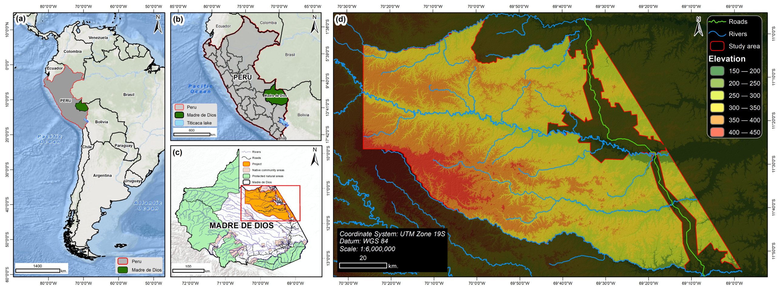
Figure 1. Location of the study area. (a) Relative location in South America; (b) Political map of Peru highlighting the Madre de Dios region; (c) Location of the evaluated area within the Tahuamanu province; (d) Detailed map of the permanent production forests under study, showing the elevation gradient, hydrological network, and main road infrastructure.
Remotesensing 18 02813 g001
Figure 2. Methodological workflow of the forest disturbance assessment in Tahuamanu (2004–2025). The diagram illustrates the integration of satellite data acquisition, spectral processing, index calculation, and the stratified area estimation process. highlighting the Madre de Dios region.
Remotesensing 18 02813 g002
Figure 3. Spatial distribution of validation sample points (n = 384) used for accuracy assessment, stratified across five ΔNDFI transition classes to ensure representativeness. (a) 2004–2015 period validated via retrospective visual interpretation (Google Earth Pro); (b) 2015–2025 period and (c) 2004–2025 period validated using field data.
Remotesensing 18 02813 g003
Figure 4. Spatiotemporal distribution of forest integrity classes and deforestation in the Tahuamanu province (2004, 2015, and 2025) displayed in scaled macro and micro disturbance panels.
Remotesensing 18 02813 g004
Figure 5. Spatial distribution of forest integrity classes and deforestation in the Tahuamanu Permanent Production Forest for 2004 (a), 2015 (b), and 2025 (c). Maps are derived from NDFI thresholds and illustrate the thematic classification for each analysis year.
Remotesensing 18 02813 g005
Figure 6. Spatial distribution of forest cover transitions and change categories derived from Δ N D F I thresholds in the Tahuamanu Permanent Production Forest for the periods: (a) 2004–2015, (b) 2015–2025, and (c) 2004–2025.
Remotesensing 18 02813 g006aRemotesensing 18 02813 g006b
Figure 7. Sankey diagram of adjusted areas for forest cover transition trajectories and change categories derived from ΔNDFI in the Tahuamanu province from 2004 to 2025.
Remotesensing 18 02813 g007
Table 1. Reflectance values for the endmembers used in the SMA model.
EndmemberBlue (B1)Green (B2)Red (B3)NIR (B4)SWIR 1 (B5)SWIR 2 (B7)
PV0.01180.03210.01550.34260.12210.0401
NPV0.03080.06260.11090.21970.28720.1797
Soil0.08260.16990.27360.40160.51040.3481
Shade0.00000.00000.00000.00000.00000.0000
Table 2. NDFI static classification ranges for forest integrity.
CategoryNDFI RangeInterpretation
Intact Forest>0.60Closed canopy; dominance of photosynthetic vegetation.
Moderate Degradation0.40 < NDFI ≤ 0.60Partial loss of leaf density; opening of clearings.
Severe Degradation0.30 < NDFI ≤ 0.40High proportion of non-photosynthetic vegetation and soil; forest infrastructure.
Deforestation≤0.30Loss of forest vegetation; complete land-use conversion.
Table 3. Classification of disturbance dynamics based on changes in ΔNDFI.
Change CategoryΔNDFI ValueInterpretation
Deforestation<−0.45Complete loss of canopy cover; transition to bare ground or grassland.
High Disturbance−0.45 < ΔNDFI ≤ −0.38Construction of logging yards and main roads.
Low Disturbance−0.38 < ΔNDFI ≤ −0.23Creation of logging clearings or narrow skid trails.
Stable (Intact Forest)−0.23 < ΔNDFI ≤ 0.20No structural changes; intact forest structure.
Spectral Recovery>0.20Closure of clearings through natural regeneration.
Table 4. Accuracy assessment and error metrics by study period.
PeriodCategoryUA (%)PA (%)Commission
Error (%)
Omission
Error (%)
2004–2015Stable (Intact Forest)98.798.71.31.3
Low Disturbance88.387.211.712.8
High Disturbance88.390.711.79.3
Deforestation97.496.22.63.8
Spectral Recovery93.493.46.66.6
Overall Accuracy93.2%
2015–2025Stable (Intact Forest)98.798.71.31.3
Low Disturbance88.388.311.711.7
High Disturbance88.389.511.710.5
Deforestation97.496.22.63.8
Spectral Recovery94.794.75.35.3
Overall Accuracy93.5%
2004–2025Stable (Intact Forest)98.798.71.31.3
Low Disturbance87871313
High Disturbance89.688.510.411.5
Deforestation96.197.43.92.6
Spectral Recovery93.493.46.66.6
Overall Accuracy93.0%
Table 5. Spatiotemporal distribution of forest integrity classes and deforestation in the Tahuamanu province for the years 2004, 2015, and 2025.
Category2004 (ha)2004 (%)2015 (ha)2015 (%)2025 (ha)2025 (%)
Intact forest831,18897.8829,54097.6816,26996.0
Moderate degradation16,9072.013,0701.523,4962.8
Severe degradation7480.117220.235050.4
Total degradation (Sum)17,6552.114,7921.727,0023.2
Deforestation9950.155060.665670.8
Total study area849,838100.0849,838100.0849,838100.0
Table 6. Annual deforestation and forest integrity degradation rates and magnitudes in the Tahuamanu province during the 2004–2015, 2015–2025, and historical 2004–2025 periods.
CategoryPeriodNet Change (ha)Annual Change (ha⋅year−1)Annual Rate (r%⋅year−1)
Intact forest2004–20151648150−0.02
2015–202513,2711327−0.16
2004–202514,919710−0.09
Moderate degradation2004–20153837349−2.31
2015–2025−10,426−10436.04
2004–2025−6589−3141.58
Severe degradation2004–2015−974−897.87
2015–2025−1783−1787.36
2004–2025−2757−1317.63
Total degradation (Sum)2004–20152863260−1.60
2015–2025−12,209−12216.20
2004–2025−9346−4452.04
Deforestation2004–2015−4511−41016.83
2015–2025−1062−1061.78
2004–2025−5573−2659.40
Table 7. Mapped and adjusted areas for forest cover transition trajectories and change categories derived from ΔNDFI in the Tahuamanu production forests across three analysis periods, with the standard error (SE) and 95% confidence interval (CI) of each adjusted area obtained from the stratified estimator.
Transition TrajectoryChange CategoryMapped Area (ha)Adjusted Area (ha)SE (ha)95% CI (ha)
2004–2015
Stable (Intact Forest)Stable (Intact Forest)821,953811,50010,677790,574–832,427
Intact Forest–DegradedLow Disturbance16,32725,45310,6934496–46,411
Intact Forest–DegradedHigh Disturbance161324684341617–3319
Intact Forest–DegradedTotal Disturbance17,94027,92110,6866976–48,866
Intact Forest–DeforestedDeforestation49164864974674–5054
Degraded–RecoveredSpectral Recovery502955534404690–6415
2015–2025
Stable (Intact Forest)Stable (Intact Forest)819,835809,38210,649788,509–830,253
Intact Forest–DegradedLow Disturbance14,60424,01710,6633118–44,916
Intact Forest–DegradedHigh Disturbance181827664431898–3634
Intact Forest–DegradedTotal Disturbance16,42226,78310,6575897–47,671
Intact Forest–DeforestedDeforestation48454788974598–4978
Degraded–RecoveredSpectral Recovery873688853968109–9661
2004–2025
Stable (Intact Forest)Stable (Intact Forest)814,873804,56910,586783,821–825,318
Intact Forest–DegradedLow Disturbance18,70027,40410,6106609–48,200
Intact Forest–DegradedHigh Disturbance205433895612290–4488
Intact Forest–DegradedTotal Disturbance20,75530,79310,60010,017–51,569
Intact Forest–DeforestedDeforestation623760151435736–6295
Degraded–RecoveredSpectral Recovery797384615297424–9497
Confidence intervals were computed as Âj ± 1.96·SE (Âj). The rare change classes carry wider intervals because their adjusted area is inferred largely from omission samples in the dominant stable-forest stratum.
Disclaimer/Publisher’s Note: The statements, opinions and data contained in all publications are solely those of the individual author(s) and contributor(s) and not of MDPI and/or the editor(s). MDPI and/or the editor(s) disclaim responsibility for any injury to people or property resulting from any ideas, methods, instructions or products referred to in the content.