


Highlights
What are the main findings?
- A convolutional neural network (CNN) approach to predicting loblolly pine canopy Leaf Area Index (CLAI), trained on LiDAR-based retrievals and using Sentinel-2 multispectral imagery, performed better than traditional linear models based on vegetation indices.
- This model was less generalizable to unobserved spatial domains; in the general case, linear modeling approaches showed lower prediction error.
What are the implications of the main findings?
- A cloud-based CNN model trained on existing LiDAR-based CLAI retrievals can effectively close gaps between infrequent data acquisitions in intensive forestry.
- Additional work, and caution, is warranted in creating generalized models for estimating stand parameters more broadly.
Abstract
Canopy Leaf Area Index (CLAI) is a stand attribute containing information on the real-time health and growth potential of managed pine plantations. Current remote sensing techniques for quantifying CLAI rely on simple linear models applied to satellite multispectral imagery, or on techniques based on light detection and ranging (LiDAR) data that are costly and less frequently collected. This study demonstrates a convolutional neural network (CNN) approach to retrieving CLAI from 10 m Sentinel-2 multispectral imagery with a model trained on gridded LiDAR-based CLAI estimates. We demonstrate large gains in accuracy with the CNN compared to traditional linear models based on vegetation indices (e.g., Simple Ratio), but also clear shortfalls in model skill when predicting “blind” in some spatial domains that were completely excluded during model training. Pixel-scale root mean squared error ranged from 0.34 to 0.64 by domain when exposed to CLAI training data from all available spatial domains, but rose to 0.58–1.74 when predicting without prior domain-specific training. Prediction accuracy was consistently lower when applied to completely unobserved USGS LiDAR-based CLAI estimates. Traditional linear models, in contrast, had the advantage of usually lower prediction error across unobserved spatial domains (0.43–1.98), but with lower maximum accuracy. These results demonstrate a potential route for deploying more complex models for LiDAR “mimicry”, e.g., between data acquisitions widely separated in time, but advocate for the development and use of more stable generalized approaches for use in unobserved managed pine stands.
1. Introduction
Leaf area index (LAI), defined as the one-sided green leaf area per unit ground area, is a central variable for characterizing the structure and functioning of forest ecosystems [1]. In managed pine plantations, LAI is closely linked to photosynthetic capacity, carbon and water fluxes, and overall stand productivity [2,3,4]. Because of its relationship to leaf area and light capture capacity, LAI has found use as a key variable when modeling carbon exchange and plant productivity [5,6] as well as serving as an indicator of stand health, vigor, and response to silvicultural treatments such as thinning, fertilization, and competition control in managed forests [7,8]. From an operational forestry perspective, the ability to monitor metrics like the LAI specifically of the crop tree canopy (CLAI) over large areas and through time could provide valuable management insights and help target silvicultural inputs [7]. In intensive forestry practice, field-based assessments of the stand canopy are done infrequently (if at all) and are impractical to implement as any routine part of stand monitoring or management planning at scale. Consequently, there is continued interest in the development of remote sensing approaches to estimate CLAI in a variety of contexts, particularly those based on satellite imagery with readily available public data sources. Such approaches for CLAI estimation would ideally provide more frequent and lower-cost information touching on stand productivity, health, and response to treatment.
Retrieval methods for LAI (either of the crop canopy alone or of the total vegetated depth) utilizing satellite multispectral imagery have been developed for a variety of vegetation contexts, including row crops and managed forests [9,10]. Several estimation models have been put forward calibrated specifically for intensively managed loblolly pine (Pinus taeda L.) plantations using imagery from both the Landsat and Sentinel-2 satellite platforms [11,12,13] and are beginning to see use in stand monitoring and management planning [7]. Such estimates rely upon relating surface reflectance spectral data to independently measured LAI or CLAI values, usually taken from the ground (e.g., light attenuation instruments, hemispherical photography) [14]. The underlying model structures that relate these two datasets are often based on linear relationships with vegetation indices (VIs), mathematical combinations of spectral band values that are selected for their sensitivity to the reflected spectra characteristic of green vegetation [15,16]. As such, any retrieval approach based on reflectance data can be expected to contain uncertainty introduced from sources including soil and understory background reflectance, variable vegetation cover fraction, instrument noise, and atmospheric distortion [17,18]. Retrieval models also tend to generalize poorly when sources of uncertainty in the reflectance data are not accounted for and when attempting to apply models trained on one forest canopy context (e.g., dominant species) to other even superficially similar contexts [19,20]. Other approaches for LAI retrieval have managed to achieve improved accuracy via more complex machine learning (ML) and other recursive modeling techniques (e.g., [21,22]) and have demonstrated progress in retrieving other biophysical metrics like aboveground biomass as well [23]. A neural network-based retrieval for producing global LAI estimates has been implemented for Sentinel-2 [24]. In all cases, retrieval models are limited in their accuracy by the quality and availability of appropriately representative training data, and by signal saturation, non-linearity, and other ambiguities in the relationships between the underlying physical attribute (e.g., CLAI) and the resulting spectral signature [25,26,27].
Airborne and more lately unmanned aerial vehicles with light detection and ranging (LiDAR) systems have emerged as particularly powerful tools for characterizing the spatial structure of forest canopies [28]. Unlike passive optical sensors, airborne LiDAR scanning actively samples the spatial distribution of physical canopy elements, providing more direct information on structural attributes—for example, quantifying canopy height and other forest inventory metrics [29,30], as well as estimates of LAI in a variety of forest types [31] due to its ability to penetrate through the vegetive canopy. Recent work specifically in loblolly pine plantations has demonstrated techniques for estimating high-resolution (10–30 m) maps of Site Index [32], CLAI and understory LAI [33], and individual tree metrics useful for stand inventory [34]. However, LiDAR has limitations versus multispectral satellite remote sensing for routine monitoring of stand CLAI. Acquisition costs remain relatively high, data processing is technically demanding, and the retrieved metrics can be sensitive to sensor configuration, pulse density, scan angle, and acquisition timing [35,36,37,38]. These constraints limit the frequency and spatial coverage of LiDAR observations, making them ill-suited as a standalone solution for large-area continuous or on-demand CLAI monitoring.
Research has begun to explore the potential for combining the structural sensitivity of LiDAR pointcloud data with the spectral and temporal coverage of optical satellite data for improving retrievals of forest attributes [39]. For example, training a model with both Sentinel-2 reflectance data and LiDAR-derived estimates of height and volume raised the accuracy of a model of growth potential for mixed-species forests across the U.S. state of Maine [40]. Another potential strategy is to use LiDAR-derived CLAI retrievals themselves as structurally informed training data for statistical or machine learning models that predict LAI from satellite reflectance. Convolutional neural networks (CNNs), in particular, offer the ability to incorporate the information contained in the two-dimensional structure of geospatial imagery data into predictive models, which may encode subtle textural cues related to canopy arrangement and shadowing (e.g., [41]). This feature is especially relevant in pine plantations, where row arrangement, crown geometry, and management-induced patterns may be detectable in imagery of high enough spatial resolution [42]. In principle, CNNs also allow complex, nonlinear relationships between spectral signatures and canopy structure to be learned, potentially improving sensitivity relative to traditional reflectance-based models. As an additional consideration, LiDAR-based CLAI retrievals (rasters) represent orders of magnitude more data points to use in training of complex CNNs, containing critical spatial context, compared to the limited ground-based point datasets used to train previous satellite-based LAI retrievals (e.g., [12]). The flexibility of complex machine learning models like CNNs also introduces risks, however. Statistical or model overfitting to the training data can result in models that perform well under familiar conditions but extrapolate poorly to new sites, management regimes, or climatic contexts [43].
The advent of cloud-based data archives of satellite imagery and the distributed computing resources to manipulate them at scale (e.g., Google’s Earth Engine [GEE] [44]) offers the prospect for creating CNN models for rapid and improved CLAI prediction at very low cost over a wide geographic and temporal sweep. Such an approach would effectively synthesize the structural information of (infrequent) LiDAR-derived CLAI and the repeated and widely available data of satellite imagery to improve the accuracy and tractability of image-like predictions of CLAI and other forest attributes. The advent of advanced image-appropriate ML techniques, the availability of complete satellite data archives and cloud-based computing resources, and the growing sophistication of LiDAR-derived canopy metrics motivate the goals of this work. This study had two primary objectives:
- We first demonstrate a CNN-based model (dubbed the “Machine Learning for Leaf Area Index”, MLAI) for pine plantations trained on a novel dataset of LiDAR-derived CLAI estimates for loblolly pine in the U.S. Southeast. This model uses Sentinel-2 L1C (top of atmosphere) multispectral data as its input and generates 10 m CLAI estimates for loblolly pine as an output. We then evaluate the predictive performance of the MLAI against traditional VI-based linear models.
- Second, we probe the extent to which the MLAI trained on a relatively limited LiDAR-derived dataset can be generalized across space, time, and scan acquisition conditions. This test is accomplished first by evaluating prediction accuracy for “blind” models denied access to training data from each discrete LiDAR acquisition domain compared with a “full” model trained with data sampled from all LiDAR domains; and second by comparing MLAI predictions to CLAI retrievals derived from publicly available pointcloud data from LiDAR acquisitions over the past several years by the U.S. Geological Survey (USGS) over various parts of the continental U.S. containing loblolly pine plantations [45].
By experimentally evaluating a CNN trained on LiDAR-based CLAI retrievals, this study seeks to clarify both the promise and the constraints of this approach. In doing so, this work aims to contribute to a more nuanced understanding of how structurally informed machine learning models can be integrated into operational CLAI estimation to provide clearer, better, and more timely information to inform the management of plantation pine forest systems.
2. Materials and Methods
2.1. Aerial LiDAR-Based CLAI Estimates
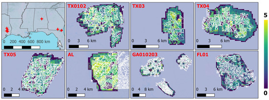
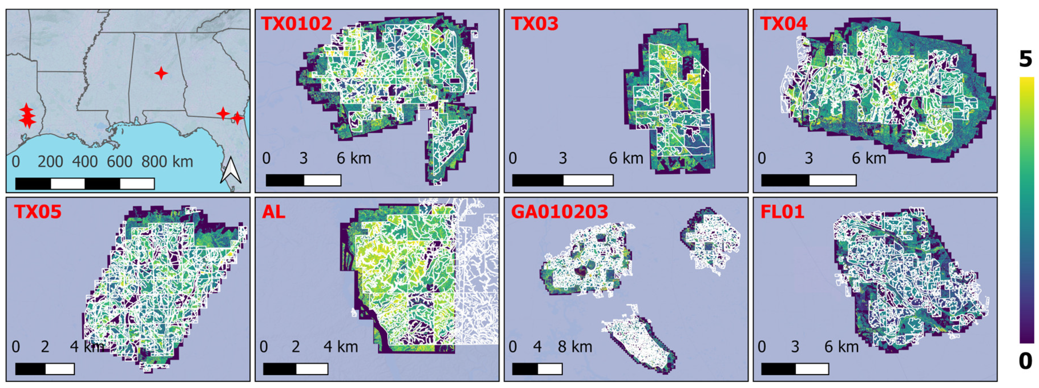
Aerial LiDAR flights covering seven roughly contiguous large spatial domains (Table 1) were conducted in January of 2018 to assess canopy and understory conditions in off-growing-season conditions: Eastern Texas (TX0102, TX03, TX04, TX05), southern Georgia (GA010203), and northeast Florida (FL01). An additional flight in January 2020 was conducted in central Alabama (AL). LiDAR acquisition domains were on the order of several km across at minimum, and separated by at least 19 km (Figure 1). The 2018 acquisitions were made from an aerial fixed-wing platform using an Optech Gemini 09SEN240 laser scanner (Teledyne Optech, Vaughan, ON, Canada) with average pulse density of 8 m−2 and 60% flight line overlap. The January 2020 acquisition was made from an aerial fixed-wing platform using a Riegl 1560ii laser scanner with average pulse density of 26 m−2 and 60% flight line overlap [46]. The LiDAR pointcloud data were processed following Sumnall et al. [33] to derive gridded (i.e., raster-based) estimates of canopy height (HT), height to live canopy (HTLC, height above ground surface at start of dominant canopy), and canopy-only LAI (CLAI, LAI between HTLC and HT) at 15–20 m spatial resolution. Estimation of CLAI with this technique relies upon the empirical linear relationship in loblolly pine stands between ground-measured canopy LAI and the log-transformed Above Below Ratio Index (ABRI), the ratio of total LiDAR returns above the identified canopy bottom height and returns at and below this height (see [33]). This LiDAR retrieval was developed to distinguish the component of LAI related only to the pine canopy from the LAI component due to understory vegetation, and was parameterized with ground-based optical measurements of LAI made using a LI-COR LAI-2200 plant canopy analyzer (LI-COR Biosciences, Lincoln, NE, USA) with diffusion correction. Thus, these LiDAR data were used in lieu of traditional ground-based field measurements.
Table 1.
Summary of loblolly stands in this study. Stand-level mean and range shown for LiDAR-derived height (HT), canopy LAI (CLAI), site age shown as median and range for stands with reliable records of establishment date. Selected clear Sentinel-2 scenes shown used for linear modeling of CLAI only. Samples refers to the number of Sentinel-2 7 × 7 pixel shards sampled for training the Machine Learning for Leaf Area Index (MLAI) model (see Section 2.2).
Figure 1.
Overview of locations of ALS LiDAR flight acquisitions in southeastern U.S. (red stars, top left), and detail of each LiDAR domain. White outlines show boundaries of managed loblolly pine stands, and color gradient shows estimated canopy LAI (CLAI) values derived from LiDAR pointclouds.
Stand boundary shapefiles identifying the location of extant loblolly plantations and other information on site history and management were obtained from Forest Productivity Coop member organizations. A total of 1104 demarcated loblolly stands had valid LiDAR coverage in the seven Sentinel-2 flightpath domains, ranging in area from <0.1 to 201 ha and in recorded time since establishment from 0 to 41 years.
2.2. Convolutional Neural Network Construction: Machine Learning for Leaf Area Index (MLAI)
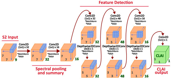
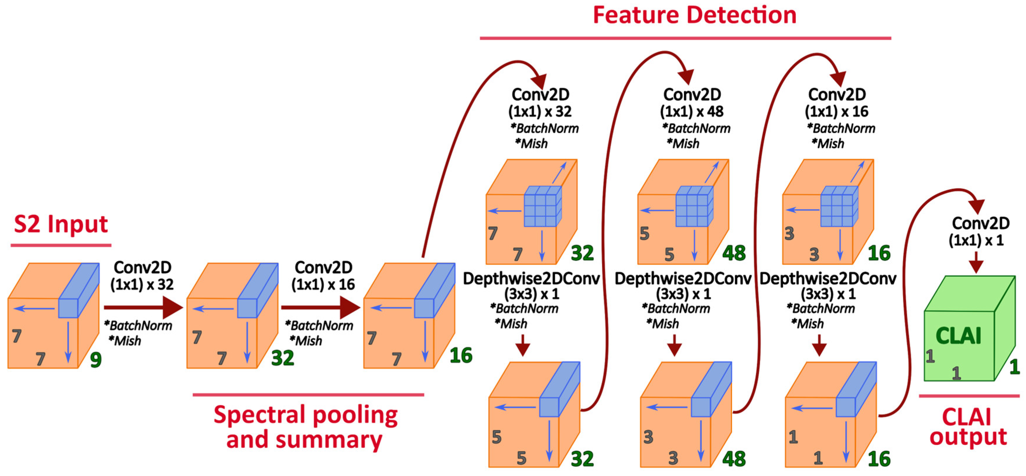
A deep convolutional neural network model (MLAI) was structured in nine successive pixel convolutional filters taking as input a raster stack of nine Sentinel-2 (S2) shortwave bands (three visible RBG bands, four NIR bands, and two SWIR bands) and trained on the LiDAR-derived CLAI rasters (this model was trained exclusively on this canopy-only LAI data, not the LAI of the full forest depth). The model started with a small image shard (7 × 7 pixels) with a central target pixel for prediction. The model first pooled and summarized spectral information through two rounds of 2D convolution across channels with a 1 × 1 pixel filter (i.e., preserving pixel spatial organization), expanding from 9 to 32 to 16 channels (Figure 2). It then passed image shards through a three-part “feature detection” cascade in which data were first pooled across channels in a 1 × 1 pixel 2D filter into a variable number of output channels (from 32 to 48 to 16 channels) followed each time by a depthwise 2D convolutional layer with a 3 × 3 pixel filter (without padding) that combined information across neighboring pixels but preserved the separate channels emerging from the previous step. After three rounds of alternating 2D convolution and depthwise 2D convolution the remaining 1 × 1 by 16 channel shard was combined linearly through a final 1 × 1 filter 2D convolution to generate the predicted CLAI value. After every convolutional step except the final, outputs were batch normalized and run through the Mish activation function [47]. The MLAI model contained approximately 5.2 k trainable parameters, and was designed to offer a relatively lightweight and computationally tractable model for rapid training and subsequent prediction maps of CLAI estimates from stock S2 top-of-atmosphere imagery. We constructed the MLAI in consultation with experts in the field of machine learning for imagery applications, with the intention of creating a model that was optimized for a straightforward regression application like the prediction of continuous stand attributes from satellite imagery. Specific evaluation of elements of the design architecture and its optimization in the MLAI was outside the scope of the study, which focused on the scope for and practical application of advanced machine learning techniques like CNN toward the improvement of tools for the prediction of management-relevant stand attributes like CLAI.
Figure 2.
Process diagram for the MLAI convolutional neural network for CLAI prediction (starts at left). Numbers in gray indicate shard pixel dimensions (X,Y), numbers in green indicate channel depth, blue boxes indicate convolution kernel (filter) type.
2.3. MLAI Model Training and Prediction
To obtain Sentinel-2 multispectral imagery data to train the model weights, we developed an automated sampling script in GEE that randomly selected shards of 7 × 7 pixel windows drawn from the Sentinel-2 L1C (top-of-atmosphere) archive overlapping known stand boundaries with LiDAR-derived LAI estimates. Training data was taken from the L1C archive because this was the only imagery readily available via GEE’s cloud-based archive at the time of model construction and training. In addition, the model structure and number of trainable parameters of the MLAI was considered to be adequate to accommodate calibration to minor atmospheric effects in otherwise nearly clear and cloud-masked scenes selected for sampling to create the training data. Sampling was controlled by first imposing a regular 0.0008° grid over each LiDAR flight domain (approximately 88 × 70 m at latitudes of test areas), then selecting a point at the center of each grid cell with a randomly imposed x and y jitter 50% the size of the grid cell, then excluding any points not falling inside the identified boundaries of a loblolly pine stand. Corresponding Sentinel-2 imagery was restricted to the acquisition period of 1 December 2017 to 1 February 2018 for all domains except Alabama (restricted to the same date range in 2019/2020) to correspond with the condition of the pine canopies when LiDAR acquisitions were done. After filtering for acquisition date, qualifying imagery was further filtered to exclude scenes with overall >20% cloudy pixels and masked for pixels with >30% cloud probability in the s2cloudless mask layer. A total of 208,407 sample shards were obtained. Raw pixel values for the surface shortwave bands as well as the LAI training values were remapped to a 0–1 scale by normalizing via empirically derived min-max limits followed by remapping over a sigmoid function. After rescaling, spectral data were augmented by randomly rotating and flipping some shards and applying random brightness and contrast changes.
Model training proceeded using the Rectified Adam protocol with Lookahead and an Exponential Decay learning schedule with a linearly increasing warmup. Training data were re-weighted according to observation frequency across the CLAI range to more heavily weight rare versus common LAI values. Training took place over 4 warmup epochs and a total of 450 training epochs, with 96 samples per batch and 2171 steps per epoch. Model specification and training were conducted in Python v3.7.16 using the Tensor Flow v2.1.0 library.
Prediction using the MLAI was performed as a cloud-based process hosted on Google’s VertexAI platform using Sentinel-2 L1C imagery hosted on Earth Engine taken from 3 December to 15 January in each LiDAR domain corresponding to the year of the initial LiDAR acquisition. Prior to use in prediction all Sentinel-2 imagery was masked for clouds by excluding scenes with total cloud cover >20% then using the s2cloudless cloud probability dataset [48,49], masking pixels with cloud probability >30% and projecting a cloud shadow mask 10 km opposite the mean solar azimuth recorded for each image. Final predicted CLAI rasters were delivered as the per-pixel mean of all predictions based on qualifying winter-scene Sentinel-2 images.
2.4. Linear Model Fitting with Vegetation Indices
For linear modeling of LiDAR-derived CLAI, top-of-atmosphere reflectance imagery (Level 1C processing) for Sentinel-2A and -2B (S2) from January 2018 and 2020, covering the area of the LIDAR flight paths in were downloaded from the Copernicus Data Space Ecosystem in August 2020 (https://browser.dataspace.copernicus.eu/), corresponding with the respective date of the LiDAR flight for each domain. A single clear scene for each domain was chosen by visual screening for minimal haze and cloud cover (Table 1). Sentinel-2 L1C data were processed using the Sen2Corr v2.8 plugin tool within the SNAP application to apply atmospheric correction to the Level 2A (L2A) surface reflectance standard, using settings for rural aerosol type, winter atmospheric profile, 331 DU ozone content, no adjacency or cirrus correction, and including orthographic correction [50]. Imagery processed to the L2A standard was used for the linear modeling portion because the additional processing was considered tractable given the smaller number of cloud-free scenes necessary to provide training data for the linear model fitting. It was further thought the fit of resulting linear models would benefit from the removal of whatever additional interference might have been present in the L1C imagery due to uncorrected atmospheric effects. The S2 imagery was filtered via the L2A scene classification layer to exclude pixels indicated to be of less than high quality and free of clouds, snow, or shadow. Reflectance data in all shortwave bands were resampled to 10 m and used to calculate a battery of 36 VIs (Table S1) following comparable previous studies in canopy structure prediction (e.g., [51]). The tasseled cap transform (TCT) was also applied to each shard to extract the brightness, greenness, and wetness features using all 13 surface shortwave and atmospheric bands, resampled to 10 m from the corresponding Level 1C scenes [52] without masking for cirrus or opaque clouds. Vegetation index and TCT values were lastly masked if outside of the middle 99.5% of their respective quantiles in each scene to eliminate high-leverage values.
LiDAR-derived CLAI estimates were resampled to a spatial resolution of 10 m and masked to exclude values over 5.0 and height values over 35 m, as these were considered ecophysiologically implausible for loblolly pine stands [4]. Sentinel-2 L2A band data, vegetation indices, and TCT features were aligned with the 10 m LiDAR-derived estimates of CLAI and total height via bilinear resampling. Pixel values were then extracted along with the area fraction of each pixel falling within the demarcated stand boundaries. Data from stands with less than ten valid LiDAR pixels (approximately 100 m2 area) were excluded from evaluation to reduce small-sample artifacts. To better match the S2 reflectance signatures of stand conditions similar to those evaluated in previous linear-modeling studies (stands at or approaching full canopy 6–18 years since establishment and LAI > 1 [11,12,33]), data were further filtered to exclude stands and pixels with indication of insufficient canopy cover. The cutoff for stand inclusion was made first based on the relationship of stand height to CLAI, excluding data from stands <4 m mean LiDAR height where mean CLAI tended to be <1. Canopy top height was used as a proxy for tree maturity instead of recorded stand age due to potential errors or ambiguities in the available records on establishment date (Figure S1). To attempt to exclude treeless intra-stand features like haul roads and skid pads, individual pixels values were masked if LiDAR height was <1 m. After excluding treeless pixels, all stands contained at least 80% or more of total pixels >1 m height. Restricting further analysis to pixels with at least 50% area coverage inside a stand boundary, this culling process resulted in 886 qualifying stands of the initial 1104, yielding approximately 1.9M qualifying pixels out of the initial 2.5M 10 m LiDAR pixels falling inside loblolly stands.
2.5. Evaluation of Model Prediction Quality
The accuracy of the MLAI model was evaluated via two approaches. In the first, the model was trained on pixel shards sampled from all seven of the available spatial domains (the “full” model version), and accuracy was evaluated by comparing predictions versus the LiDAR-derived CLAI estimates. (Note that training data sampled a small minority of LiDAR-derived central CLAI pixels in each domain; around 92% of “full”-model predictions were still being performed on previously unobserved central-pixel LiDAR-derived CLAI estimates.) In the second approach, seven separate versions of the MLAI model were trained in which samples from one entire spatial domain were excluded from each (“blind” model versions). “Blind” accuracy in this approach was assessed by examining predictions made for each domain using the model version that had no prior training exposure. This analysis was intended to explore the extent to which the MLAI model (1) could accurately mimic LiDAR-derived CLAI maps (i.e., to predict CLAI in closely similar forest types in similar regions, or in other date ranges for the same region assuming similar instrument configuration); and (2) could effectively predict CLAI maps for loblolly pine in in different areas under potentially different conditions. The second question addresses more directly the question of the potential for creating a CNN-based “universal LiDAR CLAI simulator” based on S2 reflectance data.
A similar approach was taken in evaluating CLAI models based on simple linear regression of VIs and individual spectral band data. For every regressor tested, the model was trained either on all domains or on data excluding a single domain. In the case of evaluating the LMs, model coefficients and fit metrics were evaluated as cross-validated means after splitting the data into 10 random folds, with pixel selection stratified by stand membership. This resulted in approximately 190k pixels per fold, similar to the total number of pixel shards sampled as training data for the MLAI. Minimum and maximum values of each metric across all folds were also recorded.
Predictions from the MLAI and the VI-LMs were evaluated at both the “pixel scale” of 10 m individual pixel data (100 m2) and at the “stand scale” examining the mean of pixels falling within the qualifying loblolly stands. Model error was evaluated on the basis of coefficient of determination (R2) treating the mean as the relevant Null model, per-prediction absolute error (bias), and root mean squared error (RMSE). Fit and error metrics were calculated on data restricted to the operationally significant interval of CLAI of 0.5–5.0. Data processing, analysis, and figure creation was performed in R v4.4.1 [53] using the packages dplyr v1.2.1 [54], data.table v1.16.4 [55], terra v1.8-21 [56], sf v1.0-19 [57,58], exactextractr v0.10.0 [59], and ggplot2 v4.0.3 [60].
2.6. Evaluation of MLAI Performance Against Independent USGS LiDAR-Based Estimates
MLAI predictions were also compared to CLAI estimates derived from fifteen contemporary United States Geological Survey (USGS) 3DEP LiDAR flights over the southeastern US archived for public use [61] and previously processed to reveal canopy attributes in loblolly pine stands [45]. The USGS 3DEP flights were conducted over a series of years across the US, but for this study datasets were constrained to Quality Level 2 (>2 points m−2) and to acquisitions in the winter and early spring months (December–April) of 2017–2021 to correspond with the phenologic stage of the data used for training the MLAI model. The USGS LiDAR data sets were processed using the same approach for estimating CLAI as was used to prepare the training data. Corresponding MLAI predictions were made using imagery retrieved for times and areas matching the USGS domains. A novel set of loblolly pine plantation boundaries across the southeastern US, contributed by FPC Members [45], was used to identify zones in each USGS domain that are currently under loblolly pine plantations, with a range of ages and management types (10,481 total stands falling within the 15 USGS domains).
Unlike the LiDAR datasets that were sampled training the MLAI model, CLAI estimates using publicly available USGS LiDAR point cloud data were at no point used in any prior model training. Combined with the potential variability introduced with multiple aerial platforms and instrument types, and representing point cloud data taken across novel dates, geographies, and forest conditions, the evaluation of MLAI predictions against these USGS-LiDAR-derived estimates provided a truly “blind” validation test of the correspondence of LAI estimates based on direct LiDAR-based methods and estimates based on reflectance-based models trained on prior LiDAR data.
3. Results
3.1. MLAI Prediction Accuracy at Pixel- and Stand Scale
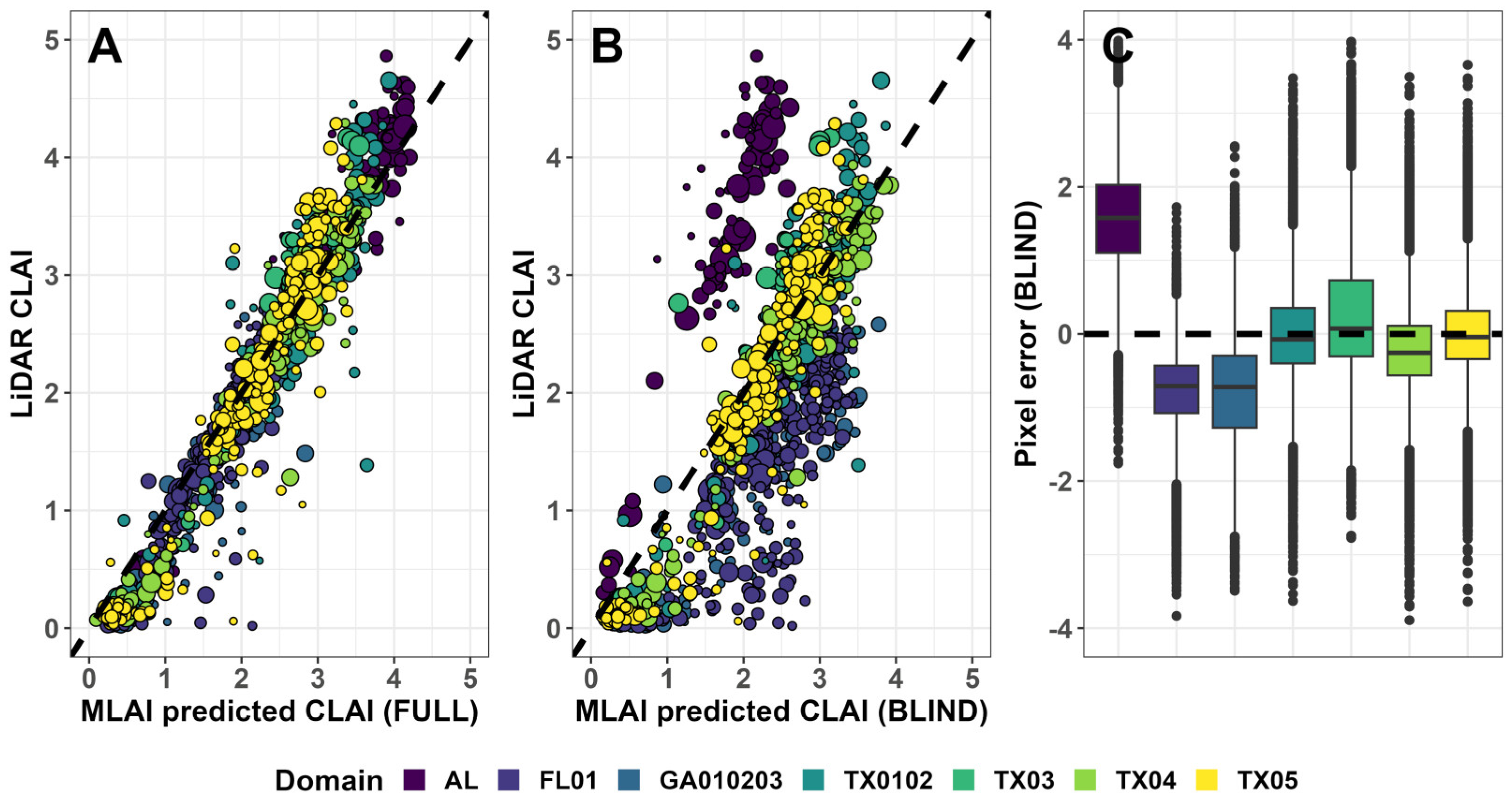
Prediction error (RMSE) was comparable across all the domains when training data included examples from each domain. However, when the training included no data from the target domain (“blind” prediction), the model showed poor predictive power in some domains (e.g., AL, GA01013, FL01) but relatively stable predictive power in others (e.g., the Texas domains) (Table 2). (Note: Negative R2 values in this context indicate that model predictions are on average less accurate than the Null model, in this case the mean of the LiDAR estimates in each domain). Poorer model predictive performance under blind conditions in some domains was often associated with larger biases (Figure 3). An examination of the distribution of pixel-scale predictions shows that in some cases the availability of even marginal additional quantities of local training data dramatically altered the behavior of the model and the resulting prediction distribution much more closely resembling the target LiDAR distribution (Figure S3). There was also evidence that the model, both full and blind versions, predicted marginally better for loblolly pine stands specifically compared to other pine species (Table S2).
Table 2.
Pixel- and stand scale prediction error metrics by LiDAR domain for MLAI CNN model trained on all domains (FULL) or with domain data excluded from training (BLIND).
Figure 3.
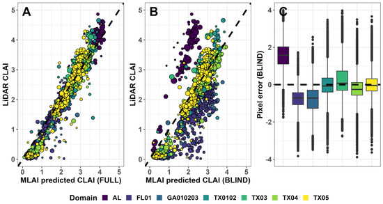
(A) Stand-mean CLAI from MLAI predictions trained on FULL datasets; (B) stand-mean predictions from BLIND models trained without any training exposure to the domains shown; (C) distribution of pixel-scale error in BLIND predictions by domain (20k randomly sampled pixels per domain). (A,B) point size indicates stand area, and dashed line shows 1:1 fit line; (C) dashed line shows pixel zero-error line.
A visual inspection of retrieved CLAI imagery shows that in domains with relatively little performance difference between blind and full model predictions (e.g., TX04), few differences are visibly noticeable in 10 m imagery (Figure S5). LiDAR-based CLAI estimates tended to capture a somewhat higher degree of variability at fine spatial scale but the MLAI- and LiDAR-based CLAI images were otherwise reasonably well matched. In contrast, in domains with poor model precision in the blind predictions (e.g., AL), there were large and systemic differences in pixel-scale CLAI predictions versus the LiDAR estimates. The change then from the blind to full MLAI predictions is more dramatic, showing a generalized rescaling of CLAI values between the two and a subsequent drop in pixel-scale error.
Stand level analysis showed similar results to pixel level error assessment, but with generally more accurate predictive performance (Table 2). As in the previous results, certain domains (i.e., AL, FL01, and GA010203) performed considerably worse due to systemic bias when the model was blinded to training data from these locations, while the prediction performance across the TX domains was relatively stable even when denied domain-specific training. Total RMSE at this scale appeared to be driven primarily by the greater bias in these blind predictions rather than high unbiased stochastic error (Figure S2). At both the pixel- and stand scale, prediction error by the model tended to be higher at the extreme ends of the CLAI range. Distributions of MLAI predictions scaled to the stand-mean level showed similar mis-match patterns in blind prediction as at the pixel scale predictions in each domain (Figure S4).
3.2. MLAI CLAI Predictions vs. USGS-LiDAR Derived Estimates
There was general agreement between USGS LiDAR-derived CLAI estimates and MLAI predictions in relative CLAI size but a clear bias in the estimated absolute magnitude of CLAI (Table 3). A simple linear model relating the MLAI-based and USGS LiDAR-based estimates at the pixel scale did not show an especially strong fit (R2 0.44), with a slope of 0.58 and with an intercept of 0.37 also indicating a consistent bias across spatial domains and across the operationally significant CLAI range. As in the previous analysis, there was variability in agreement between the MLAI and USGS estimates across the 15 domains but generally poorer fit than with the foundational LiDAR training datasets (Table 3). RMSE was generally somewhat less than 1.0 in comparing the two datasets, and R2 was generally low to negative (i.e., poorer performance than the Null/Mean estimate), though differing greatly among domains. Model fit metrics at the stand-mean level showed the same general pattern as at the pixel scale. Qualitatively, the relative magnitude of MLAI-based estimates tracked with CLAI levels in the USGS LiDAR estimates, but did not predict the same high intra-stand variability present in the original LiDAR-based estimates (Figure S6). Predictions from the S2-based MLAI model appeared to correlate with CLAI predictions from a previously reported VI-based CLAI model [12] better than the USGS LiDAR-based CLAI estimates (Figure S7). This pattern indicates that though the correspondence between MLAI- and USGS LiDAR-based estimates was relatively weak, the MLAI estimates were still sensitive to vegetation greenness levels (SR) even in completely unobserved forest canopies (Supplemental S3).
Table 3.
Error in LAI estimate between USGS-based and MLAI-based LAI predictions. Analysis restricted to pixels with at least 50% area inside identified stands, stands with at least 10 valid pixels of retrieved data, and LAI range of 0.5–5.0.
3.3. Relative Performance of Linear Regression Models Using VIs
In contrast to the pattern seen in the MLAI outputs, LM-VI model prediction performance was not dramatically lower on average when model training was blinded by domain, and blind RMSE for the best linear models was somewhat lower in some domains than comparable blind predictions from the MLAI. However, while model performance was also improved by exposure to domain-specific training data this improvement was modest compared to the improvement in the MLAI predictions, and model fit metrics in the best LMs were considerably lower than for the MLAI with full domain training. Mean bias was very low for predictions from the blinded models, and was, as expected, near 0 with full domain training.
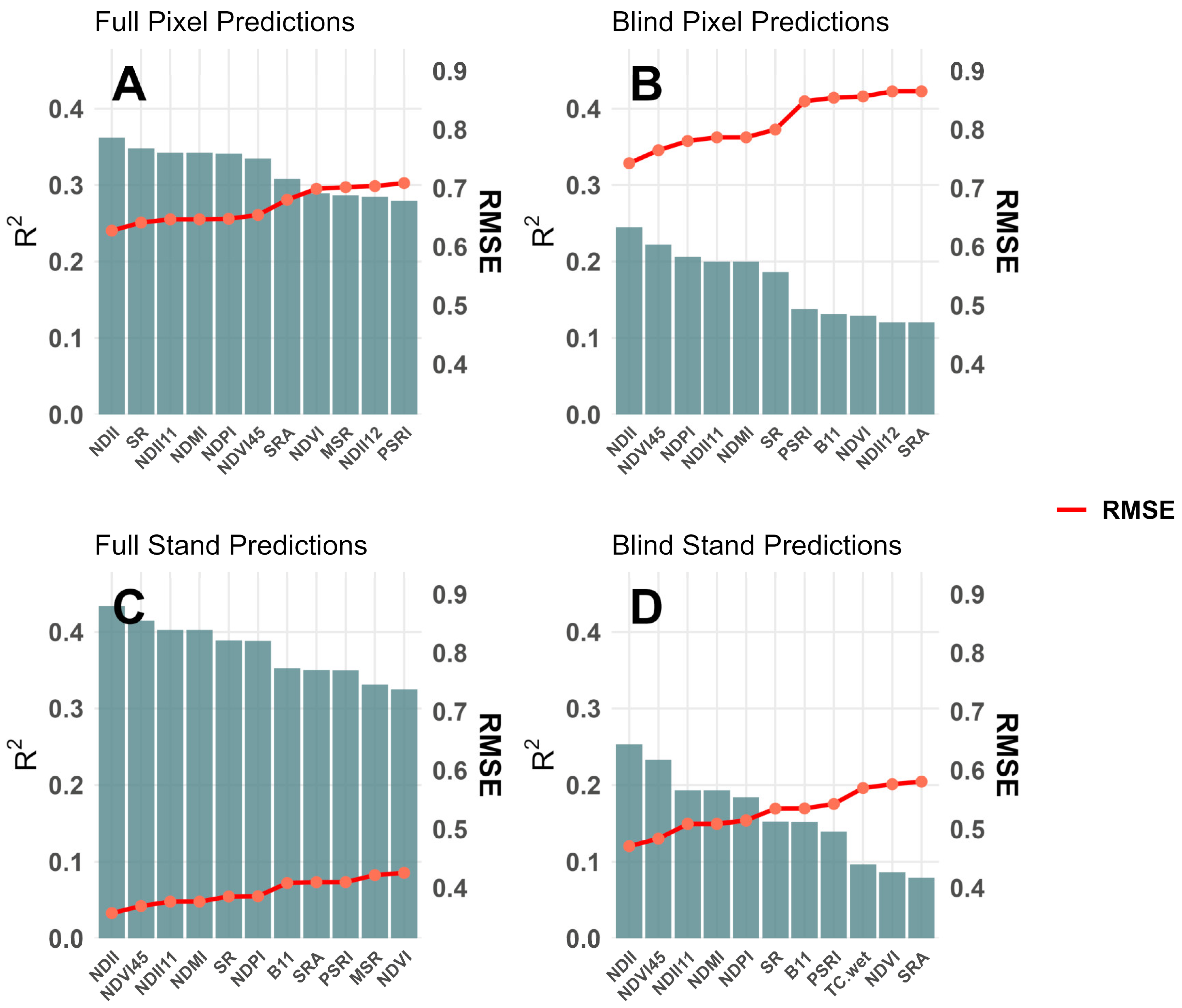
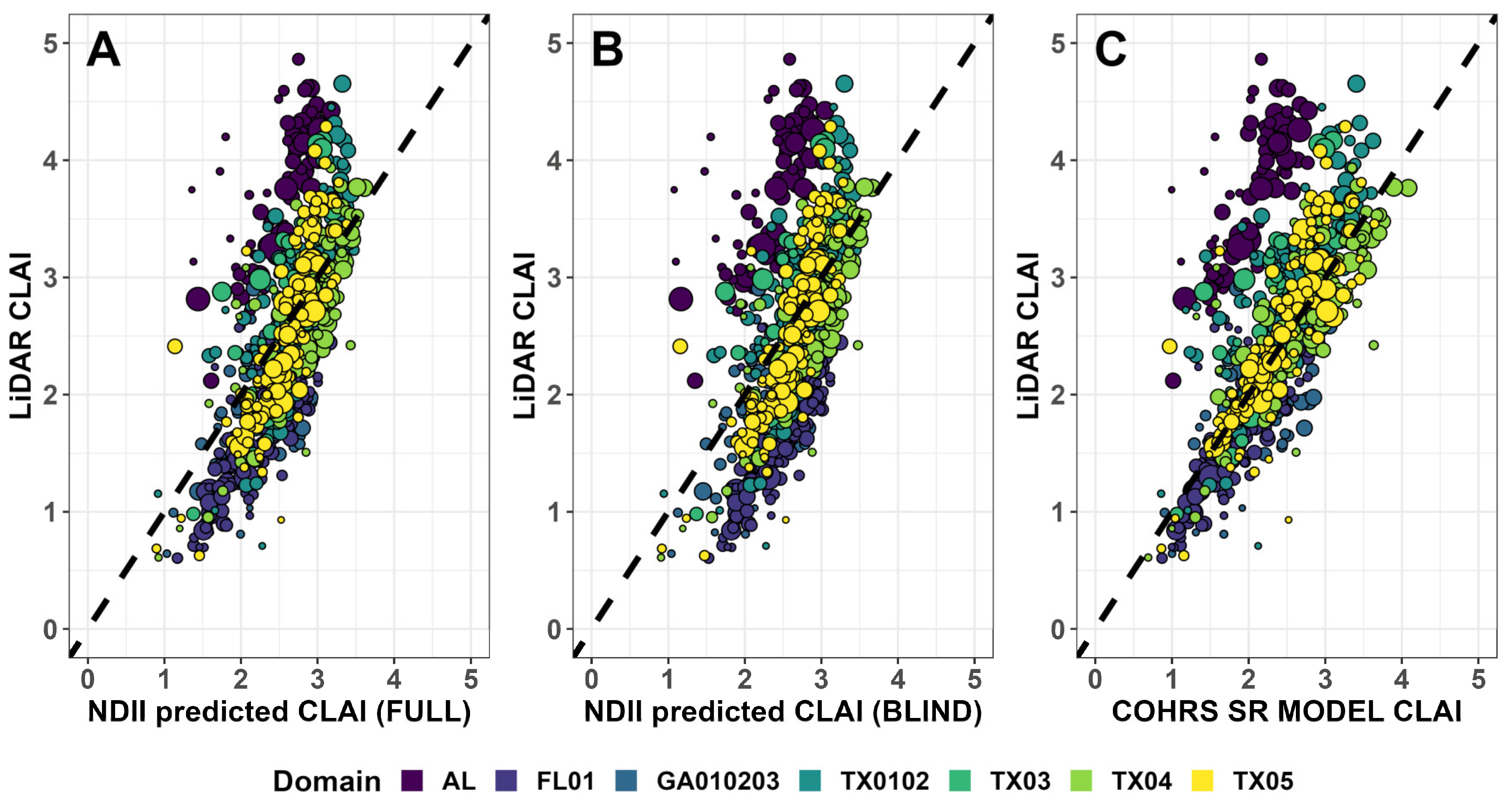
Stand-mean predictions were generally more accurate than the underlying pixel-scale predictions in both full and blind models, and all scales and training datasets shared the same top six ranked predictors: NDII, NDVI45, NDII11, NDMI, SR, and NDPI (Figure 4; see Table S1 for definitions). The best performing model (in both blind and full training) used the NDII, evaluated at both pixel and stand-mean scales. This linear model showed the same pattern of worse performance when blinded to specific domain training data, as with blind predictions in the MLAI, but usually less change in fit quality when provided training data across all domains (Figure 5).
Figure 4.
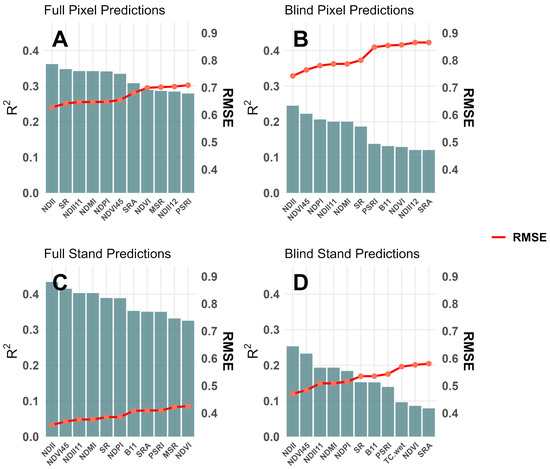
The top 11 models (by lowest RMSE) for single LMs predicting CLAI. Bars show R2, red line shows RMSE. (A): Pixel-scale Full; (B): Pixel-scale Blind; (C): Stand-scale Full; (D): Stand-scale Blind.
Figure 5.
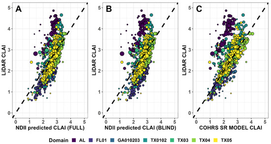
Stand-scale predictions for linear model based on (A) NDII with Full domain training, (B) NDII with Blind domain training; (C) Cohrs et al. [12] SR-based model. Points scaled to size of stand, dotted line shows 1:1 fit.
The best-fit coefficients for this model (full training across all domains), using the Normalized Difference Infrared Index (NDII [62]), was:
Prediction error at pixel scale for this model across all domains, with full training data, was RMSE 0.63, and coefficient of determination 0.36. Domain-average blind RMSE for this model ranged from 0.43 to 1.99. Models based on the Simple Ratio (SR) were also typically ranked highly for fit metrics among other single-VI predictors, as indicated in prior studies [11,12,63] (Figure 4). By some metrics the previously published SR-based LM for Sentinel-2 [12], trained on different CLAI data, was less susceptible to the influence of domains with poor model fit when trained with our LiDAR-based CLAI data (e.g., AL) (Figure 5; see Supplemental S4 for further discussion of linear model fits).
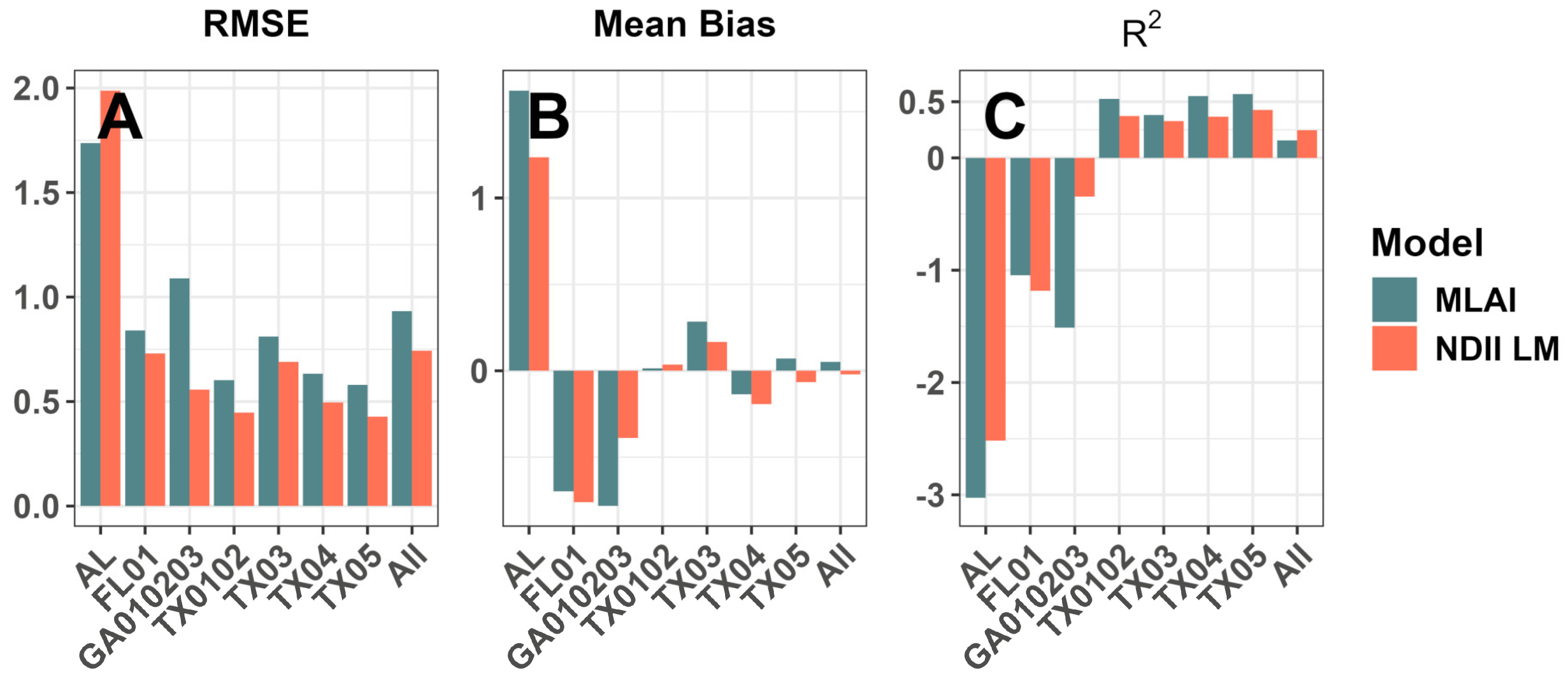
A comparison of error in domain-blind predictions between the best-performing NDII LM and the MLAI model showed comparable variable advantages in certain domains (Figure 6). Both models showed considerably worse blind prediction error in the same specific domains (AL, GA010203, FL01) and similar tendencies to either consistently over- or under-estimate. The NDII-based model had somewhat lower domain-blind RMSE in all domains except AL. Neither the NDII-based model nor the MLAI consistently performed better in terms of mean bias in different domains. In the low-accuracy domains, blind predictions from the NDII model were somewhat closer to the observed CLAI, but in the TX domains the MLAI model predicted somewhat more accurately. Results were comparable at the stand scale, with the NDII model showing a slightly greater RMSE advantage in the NDII model across domains except for AL (Figure S9).
Figure 6.
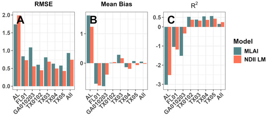
Comparative metrics of blind pixel-scale prediction accuracy in the NDII-based LM and the MLAI CNN model, by domain: (A) RMSE; (B) mean bias; (C) coefficient of determination (R2).
4. Discussion
A great deal of research has lately taken place in the field of image processing for forest attribute retrieval and demarcation, including on the use of CNNs for these applications. Studies have adapted the UNet or other CNN architectures for estimating a variety of forest attributes: boreal forest height in using S2 and SAR data [64]; boreal forest height and cover using high-resolution multispectral and X-band radar [65]; forest height across country-sized spatial domains using S2 data [66]; classifying forest cover at the species level [67]; and segmentation of imagery to segment forests and recent deforestation in contrasting biomes [68,69]. Other studies have examined the potential for combining LiDAR and optical imagery to enhance the ability to retrieve LAI in North American temperate forest [70], the combination of S2 and SAR for LAI estimation of forests in Iran [71], and the use of space-borne LiDAR returns as training for a Landsat-based canopy height retrieval [72]. To our knowledge, no study has yet attempted to use a CNN approach with LiDAR-based training data for the specific application of detecting a canopy structural attribute such as LAI, as in this study.
The MLAI is a relatively lightweight CNN that is comparatively simple compared to commonly used CNNs for image segmentation and classification tasks, e.g., UNet [73], which contains typically many millions of parameters compared to the MLAI’s few thousand. Even so, with domain-specific training the MLAI was able to effectively mimic the LiDAR-based estimates across a wide range of CLAI and other stand structural variables. The relative simplicity of the MLAI contributes to some attractive features: It was relatively quickly trained using the available LiDAR-based CLAI rasters, on the order of 1–2 days using a single high-performance computing node without significant GPU support. The MLAI also generated predictions quickly when running on lower-power cloud-based prediction nodes: Areas of interest with scales of dozens of km (i.e., the LiDAR domains themselves) could be predicted in less than ten minutes with models hosted on VertexAI fed with imagery from Earth Engine, at a nominal cost of a few US dollars per retrieval. Using an approach similar to MLAI, such a modeling framework could be useful for forest managers in filling in spatial or temporal gaps in coverage between LiDAR flights. For example, if a manager has access to LiDAR data collected infrequently an MLAI-like model, trained on LiDAR-based CLAI features, could fill wall-to-wall CLAI predictions for the same domain in subsequent years and in nearby stands without LiDAR data.
It was apparent from testing that attempting to apply the MLAI in areas to spatial domains not sampled for training data for the model left the user at risk of producing poor quality predictions. For the case of the AL domain, LiDAR-based CLAI values tended to be higher than in other domains, stands tended to be somewhat older and taller, and the ALS acquisition details were somewhat different than the other 2018 scans. The other two domains with poorer “blind” prediction accuracy (FL01 and GA010203) were scanned under similar sensor set-ups to the other domains, but in these domains stands tended to be younger and shorter stature, with notably lower CLAI. In both cases, it is possible that the somewhat unusual canopy conditions of stands in these domains, compared to conditions in the bulk of the LiDAR training data from other domains, might have contributed to the lack of fit when the MLAI did not have any training exposure. The higher point density for the AL scan might also have tended to bias the CLAI retrievals there higher due to unknown interfering factors. Further, the presence of error in the underlying retrieval model relating the LiDAR pointcloud features with the (benchmark) ground-based canopy LAI measures [33] also implies that the LiDAR-based CLAI estimates may vary somewhat versus the canopy structural attributes responsible in part for creating the reflectance signal captured by Sentinel-2. In such conditions, poor “blind” prediction performance by the MLAI might reflect some combination of a lack of fit in the CNN as well as relatively poor retrieval of CLAI using the LiDAR pointcloud data. The risk of poor zero-training predictive performance (i.e., poor correspondence to the LiDAR-based CLAI values) in the MLAI was moreover not easily anticipated beforehand. The low-accuracy domains, while perhaps somewhat systematically different, were topographically similar and still contained numerous stands of the same general condition as those distributed across the broader training data. With no clear means of defining what kinds of forest context or other factors (e.g., instrument suite, soil background) were likely to be well- versus poorly- generalized to, it remains unclear how error in the predictions can be anticipated or partitioned, nor is it clear what the anticipated error would be in predictions from CNN-based models like the MLAI when predicted on data outside its training data spatial domain.
Though training data for the MLAI was sparsely sampled from each LiDAR spatial domain, the addition of even relatively small amounts of domain-specific data dramatically improved prediction performance in certain “difficult” domains—a specific example of the problem of diminished performance under “domain shift” in applications of remote sensing [74]. Simpler models with reduced predictive power may tend to also generalize to different domains more readily than complicated models [75], though the lower number of trainable parameters in the MLAI makes it unlikely it was capable of purely “memorizing” CLAI values. In this study, predictions from VI-LMs were not as much degraded by lack of access to domain-specific training data (models were more “generalized” across domains; RMSE differences between FULL and BLIND model predictions were lower) but were also never as accurate as the MLAI with domain-specific training exposure. The difference in prediction performance in the two approaches across domains is a concrete demonstration of the bias-vs-variance tradeoff in model construction [76].
The traditional approach in loblolly pine forestry up to now (i.e., linear models of CLAI based on VIs) did appear to generalize more readily across domains. The predictions from these models were less accurate overall but were of similar quality irrespective of the domain to which they were applied. We find that a VI-LM using NDII (and fit using a much larger amount of training data) performed marginally better than a LM using SR, which was previously favored. With that said, the most recent prior published CLAI model for loblolly pine using SR values from S2 imagery [12], trained on independent LICOR-based CLAI measures, rendered the lowest-error blind predictions for the LiDAR-based CLAI estimates across all domains (Supplemental S4). Our findings also confirm the relatively strong relationship between satellite SR measures and CLAI, in this study estimated via LiDAR-based methods but in others estimated via ground-based measurements.
More generally, the highest-performing single-term LMs all used VIs or bands sensitive to the near-infrared and shortwave infrared spectra, which likely contain the most relevant information in predicting canopy photosynthetic attributes [11,15,51,77]. Moreover, the MLAI predictions themselves tended to correlate with SR values, implying that these traditional reflectance patterns must also be influential in the more complicated CNN weightings. However, though MLAI estimates often generally followed traditional VI-based estimates, the “difficult” LiDAR domains in the training set (e.g., AL) and in the USGS LiDAR data generated CLAI estimates that differed substantially from any of the reflectance-based estimates, even those based on SR. It is further notable that the distribution shapes of LiDAR-derived CLAI from some of the poorly predicted domains were quite distinct from the better-behaved domains. It is unknown if the “difficult” USGS domains represented genuinely divergent conditions in canopy, background, or other factors, or if these instead represented the limitations of the LiDAR CLAI retrieval technique itself. The low slope value between the MLAI- and USGS-based CLAI estimates in those domains (0.58) indicate strongly that whatever reflectance signatures the MLAI was trained to in the original ALS data, there was systematic disagreement with the USGS-based CLAI estimates. (It is noted that the point density of the USGS ALS acquisitions also tended to be lower than those used to supply training data in this study.) The question of how to partition errors in model fit between error in the training data (of whatever source) and lack of model fit is an ongoing issue in remote sensing science [78]. Assuming error is present in the LiDAR-derived training data, the reported RMSE for the MLAI and VI-LMs in this study may be biased upwards, and the revealed model relative rankings may be unstable [79]. Correctives have been proposed to better estimate prediction error if training data error is quantified [80]; it may also be possible to adapt learning approaches to use training processes robust to label noise, and/or train models that output confidence distributions rather than hard predictions [81]. The scope of the current project prevented further exploration of the relative influence of error in the training data versus error in the model fit, both of which are likely present. We, however, note that this remains an outstanding aspect of efforts to use remote sensing data in practical applications such as explored in this work.
The issue of uncertainty in the quality of the available training/validation data also raises the broader problem of deciding which instrument or approach for generating CLAI estimates should be considered the “authoritative” source. Since LAI is very seldom measured directly, even for ground-based methods (e.g., attenuation), in a sense there exist very little “error-free” LAI datasets to train with, and every LAI measurement is in reality a retrieved estimate based on a further underlying empirical- or process-based model containing some amount of prediction error. Thus, grappling with the issue of uncertainty in both the training data and the resulting model outputs seems to be an inevitable task in making further progress with remote sensing-based forest monitoring.
Future research in the area could explore the applicability of machine-vision approaches to higher-density LiDAR pointcloud data taken from unmanned aerial vehicles [82], and the potential for the inclusion of additional kinds of imagery data such as synthetic aperture radar or hyperspectral reflectance [51,83]. There is also the potential that other recursive ML techniques, including some newer approaches based on gradient boosting and Bayesian regularized neural networks, more diverse model ensembles, and/or multi-sensor inputs, might strike a different compromise between spatial generalizability and improved prediction accuracy [84]. The focus of this modeling work on winter canopy condition, and the use of corresponding wintertime imagery, may have worked to minimize the influence of deciduous competing vegetation on the overall spectral signatures. However, it also raises the possibility of stronger atmospheric and sun-angle effects on the observed spectra that may vary significantly from pine canopy observed in other seasons [85]. Future work to develop canopy-attribute models based on satellite multispectral imagery should consider these potential seasonal effects, and the possibility of better model fits at different times of year, while also controlling for interference from competing vegetation.
5. Conclusions
We demonstrated a CNN-based model for CLAI in loblolly pine plantations trained on rasters of CLAI estimated from LiDAR and Sentinel-2 imagery. This model showed increased prediction accuracy compared to the traditional approach of linear models based on single VIs, though accuracy advantages disappeared when the training data included no examples from the specific spatial domain targeted. Analysis of the results confirmed the sensitivity of satellite-based near- and shortwave infrared to a LiDAR-estimated vegetation structural component like CLAI. The approach demonstrated in this work could offer a tool for filling temporal and spatial gaps between infrequent LiDAR aerial scans with readily available satellite imagery, especially in a cloud-based data and computing environment. However, uncertainty in the error properties of the underlying LiDAR-derived training data and unpredictable generalization capacity urge caution when using CNN-based models such as this for CLAI prediction outside of biophysical contexts and spatial domains well represented in the training data.
Supplementary Materials
The following supporting information can be downloaded at: https://www.mdpi.com/article/10.3390/rs18162814/s1.
Author Contributions
Conceptualization, A.T. and R.L.C.; methodology, A.T.; software, A.T.; validation, A.T. and M.J.S.; formal analysis, A.T.; investigation, A.T.; resources, R.L.C.; data curation, A.T., R.L.C. and M.J.S.; writing—original draft preparation, A.T.; writing—review and editing, A.T., R.L.C. and M.J.S.; visualization, A.T.; supervision, R.L.C.; project administration, R.L.C.; funding acquisition, R.L.C. All authors have read and agreed to the published version of the manuscript.
Funding
This work was supported by the Center for Advanced Forestry Systems funded under the U.S. National Science Foundation award 1916552, with additional support provided by the Forest Productivity Cooperative at NCSU.
Data Availability Statement
The datasets analyzed and generated during this study are available from the corresponding author at the discretion of the co-authors. Data that will be released include summary data and datasets with spatial identifiers removed, as well as relevant code base. Raw spatial coordinates for specific stand locations and privately acquired data are not publicly available due to confidentiality agreements with landowners.
Acknowledgments
The authors gratefully acknowledge Valerie Pasquarella and Christopher Brown at Google for critical technical and strategic input on CNN model development and Earth Engine integration.
Conflicts of Interest
The authors declare no conflicts of interest.
Abbreviations
The following abbreviations are used in this manuscript:
| CLAI/LAI | (Canopy) Leaf Area Index |
| CNN | Convolutional Neural Network |
| LiDAR | Light Detection and Ranging |
| MLAI | Machine Learning for Leaf Area Index |
| NIR/SWIR | Near-Infrared/Shortwave Infrared |
| RMSE | Root Mean Squared Error |
| USGS | United States Geological Survey |
| VI | Vegetation Index |
References
- Parker, G.G. Tamm Review: Leaf Area Index (LAI) Is Both a Determinant and a Consequence of Important Processes in Vegetation Canopies. For. Ecol. Manag. 2020, 477, 118496. [Google Scholar] [CrossRef] [Scilit]
- Fox, T.R.; Allen, H.L.; Albaugh, T.J.; Rubilar, R.; Carlson, C.A. Tree Nutrition and Forest Fertilization of Pine Plantations in the Southern United States. South. J. Appl. For. 2007, 31, 5–11. [Google Scholar] [CrossRef] [Scilit]
- Luo, Y.; Medlyn, B.; Hui, D.; Ellsworth, D.; Reynolds, J.; Katul, G. Gross Primary Productivity in Duke Forest: Modeling Synthesis of CO2 Experiment and Eddy-Flux Data. Ecol. Appl. 2001, 11, 239–252. [Google Scholar] [CrossRef] [Scilit]
- Vose, J.M.; Allen, H.L. Leaf Area, Stemwood Growth, and Nutrition Relationships in Loblolly Pine. For. Sci. 1988, 34, 546–563. [Google Scholar] [CrossRef] [Scilit]
- Bi, W.; He, W.; Zhou, Y.; Ju, W.; Liu, Y.; Zhang, X.; Wei, X.; Cheng, N. A Global 0.05° Dataset for Gross Primary Production of Sunlit and Shaded Vegetation Canopies from 1992 to 2020. Sci. Data 2022, 9, 233. [Google Scholar] [CrossRef] [Scilit] [PubMed]
- Mahadevan, P.; Wofsy, W.C.; Matross, D.M.; Xiao, X.; Dunn, A.L.; Lin, J.C.; Gerbig, C.; Munger, J.W.; Chow, V.Y.; Gottlieb, E.W. A Satellite-Based Biosphere Parameterization for Net Ecosystem CO2 Exchange: Vegetation Photosynthesis and Respiration Model (VPRM). Glob. Biogeochem. Cycles 2008, 22, 2005. [Google Scholar] [CrossRef] [Scilit]
- Cohrs, C.W.; Lyons, A.; Albaugh, T.J.; Carter, D.R.; Campoe, O.C.; Rubilar, R.A.; Sumnall, M.; Trlica, A.; Corrao, M.V.; Virk, S.; et al. Precision Forestry in Actively Managed Loblolly Pine Plantations: Leaf Area Index Response One Growing Season Following a Variable-Rate Fertilization. For. Ecol. Manag. 2025, 595, 122989. [Google Scholar] [CrossRef] [Scilit]
- House, M.N.; Wynne, R.H.; Thomas, V.A.; Cook, R.L.; Carter, D.R.; Mullekom, J.H.; Rakestraw, J.; Schroeder, T.A. Effects of establishment fertilization on Landsat-assessed leaf area development of loblolly pine stands. For. Ecol. Manag. 2024, 556, 121655. [Google Scholar] [CrossRef] [Scilit]
- Cañete-Salinas, P.; Zamudio, F.; Yáñez, M.; Gajardo, J.; Valdés, H.; Espinosa, C.; Venegas, J.; Retamal, L.; Ortega-Farias, S.; Acevedo-Opazo, C. Evaluation of Models to Determine LAI on Poplar Stands Using Spectral Indices from Sentinel-2 Satellite Images. Ecol. Model. 2020, 428, 109058. [Google Scholar] [CrossRef] [Scilit]
- Viña, A.; Gitelson, A.A.; Nguy-Robertson, A.L.; Peng, Y. Comparison of Different Vegetation Indices for the Remote Assessment of Green Leaf Area Index of Crops. Remote Sens. Environ. 2011, 115, 3468–3478. [Google Scholar] [CrossRef] [Scilit]
- Blinn, C.E.; House, M.N.; Wynne, R.H.; Thomas, V.A.; Fox, T.R.; Sumnall, M. Landsat 8 based leaf area index estimation in loblolly pine plantations. Forests 2019, 10, 222. [Google Scholar] [CrossRef] [Scilit]
- Cohrs, C.W.; Cook, R.L.; Gray, J.M.; Albaugh, T.J. Sentinel-2 Leaf Area Index Estimation for Pine Plantations in the Southern United States. Remote Sens. 2020, 12, 1406. [Google Scholar] [CrossRef] [Scilit]
- Kinane, S.M.; Montes, C.R.; Albaugh, T.J.; Mishra, D.R. A model to estimate leaf area index in loblolly pine plantations using Landsat 5 and 7 images. Remote Sens. 2021, 13, 1140. [Google Scholar] [CrossRef] [Scilit]
- Bréda, N.J.J. Ground-Based Measurements of Leaf Area Index: A Review of Methods, Instruments and Current Controversies. J. Exp. Bot. 2003, 54, 2403–2417. [Google Scholar] [CrossRef] [Scilit] [PubMed]
- Kira, O.; Nguy-Robertson, A.L.; Arkebauer, T.J.; Linker, R.; Gitelson, A.A. Informative Spectral Bands for Remote Green LAI Estimation in C4 and C4 Crops. Agric. For. Meteorol. 2016, 218–219, 243–249. [Google Scholar] [CrossRef] [Scilit]
- Xue, J.; Su, B. Significant Remote Sensing Vegetation Indices: A Review of Developments and Applications. J. Sens. 2017, 2017, 1353691. [Google Scholar] [CrossRef] [Scilit]
- Lunetta, R.S.; Congalton, R.G.; Fenstermaker, L.; Jensen, J.R.; McGwire, K.C.; Tinney, L.R. Remote Sensing and Geographic Information System Data Integration: Error Sources and Research Issues. Photogramm. Eng. Remote Sens. 1991, 57, 677–687. [Google Scholar]
- Roy, D.P.; Zhang, H.K.; Ju, J.; Gomez-Dans, J.L.; Lewis, P.E.; Schaaf, C.B.; Sun, Q.; Li, J.; Huang, H.; Kovalskyy, V. A general method to normalize Landsat reflectance to nadir BDRF adjusted reflectance. Remote Sens. Environ. 2016, 176, 255–271. [Google Scholar] [CrossRef] [Scilit]
- Peduzzi, A.; Allen, H.L.; Wynne, R.H. Leaf Area of Overstory and Understory in Pine Plantations in the Flatwoods. South. J. Appl. For. 2010, 34, 154–160. [Google Scholar] [CrossRef] [Scilit]
- Verrelst, J.; Camps-Valls, G.; Muñoz-Marí, J.; Rivera, J.P.; Veroustraete, F.; Clevers, J.G.P.W.; Moreno, J. Optical Remote Sensing and the Retrieval of Terrestrial Vegetation Bio-Geophysical Properties—A Review. ISPRS J. Photogramm. Remote Sens. 2015, 108, 273–290. [Google Scholar] [CrossRef] [Scilit]
- Houborg, R.; McCabe, M.F. A Hybrid Training Approach for Leaf Area Index Estimation via Cubist and Random Forests Machine-Learning. ISPRS J. Photogramm. Remote Sens. 2018, 135, 173–188. [Google Scholar] [CrossRef] [Scilit]
- Zhang, Z.; Xin, Q.; Li, W. Machine Learning-Based Modeling of Vegetation Leaf Area Index and Gross Primary Productivity across North America and Comparison with a Process-Based Model. J. Adv. Model. Earth Syst. 2021, 13, e2021MS002802. [Google Scholar] [CrossRef] [Scilit]
- Chen, L.; Ren, C.; Zhang, B.; Wang, Z.; Xi, Y. Estimation of Forest Above-Ground Biomass by Geographically Weighted Regression and Machine Learning with Sentinel Imagery. Forests 2018, 9, 582. [Google Scholar] [CrossRef] [Scilit]
- Weis, M.; Baret, F. S2ToolBox Level 2 Products: LAI, FAPAR, FCOVER, version 1.1. 2016. Available online: http://step.esa.int/docs/extra/ATBD_S2ToolBox_L2B_V1.1.pdf (accessed on 1 December 2020).
- Gao, S.; Zhong, R.; Yan, K.; Ma, X.; Chen, X.; Pu, J.; Gao, S.; Qi, J.; Yin, G.; Myneni, R.B. Evaluating the Saturation Effect of Vegetation Indices in Forests Using 3D Radiative Transfer Simulations and Satellite Observations. Remote Sens. Environ. 2023, 295, 113665. [Google Scholar] [CrossRef] [Scilit]
- Huete, A.R.; Liu, H.Q.; Leeuwen, W.J.D. The Use of Vegetation Indies in Forested Regions: Issues of Linearity and Saturation. In Proceedings of the IGARSS’97, 1997 IEEE International Geoscience and Remote Sensing Symposium Proceedings. Remote Sensing—A Scientific Vision for Sustainable Development, Singapore, 3–8 August 1997; Volume 4, pp. 1966–1968. [Google Scholar] [CrossRef] [Scilit]
- Mas, J.F.; Flores, J.J. The Application of Artificial Neural Networks to the Analysis of Remotely Sensed Data. Int. J. Remote Sens. 2008, 29, 617–633. [Google Scholar] [CrossRef] [Scilit]
- Wang, Y.; Kukko, A.; Hyyppä, E.; Pyörälä, J.; Lehtomäki, M.; Issaoui, A.E.; Yu, X.; Kaartinen, H.; Liang, X.; Hyyppä, J. Seamless Integration of Above- and under-Canopy Unmanned Aerial Vehicle Laser Scanning for Forest Investigation. For. Ecosyst. 2021, 8, 10. [Google Scholar] [CrossRef] [Scilit]
- Hyyppä, J.; Hyyppä, H.; Litkey, P.; Yu, X.; Haggrén, H.; Rönnholm, P.; Pyysalo, U.; Pitkänen, J.; Maltamo, M. Algorithms and Methods of Airborne Laser Scanning for Forest Measurements. In Proceedings of the Laser-Scanners for Forest and Landscape Assessment—Instruments, Processing Methods, and Applications; Koch, B., Spiecker, H., Weinacker, H., Eds.; International Society for Photogrammetry and Remote Sensing: Hannover, Germany, 2004; pp. 82–89. [Google Scholar]
- White, J.C.; Coops, N.C.; Wulder, M.A.; Vastraranta, M.; Hilker, T.; Tompalski, P. Remote Sensing Technologies for Enhancing Forest Inventories: A Review. Can. J. Remote Sens. 2016, 42, 619–641. [Google Scholar] [CrossRef] [Scilit]
- Wang, Y.; Fang, H. Estimation of LAI with LiDAR Technology: A Review. Remote Sens. 2020, 12, 3457. [Google Scholar] [CrossRef] [Scilit]
- Ribas-Costa, V.; Gastón-Gonzáles, A.; Bloszies, S.A.; Henderson, J.D.; Trlica, A.; Carter, D.R.; Rubilar, R.A.; Campoe, O.C.; Albaugh, T.J.; Cook, R.L. Nature vs. Nurture: Drivers of Site Productivity in Loblolly Pine (Pinus taeda L.) Forests in the Southeastern U.S. For. Ecol. Manag. 2024, 572, 122334. [Google Scholar] [CrossRef] [Scilit]
- Sumnall, M.J.; Trlica, A.; Carter, D.R.; Cook, R.L.; Schulte, M.L.; Campoe, O.C.; Rubilar, R.A.; Wynne, R.H.; Thomas, V.A. Estimating the Overstory and Understory Vertical Extents and Their Leaf Area Index in Intensively Managed Loblolly Pine (Pinus taeda L.) Plantations Using Airborne Laser Scanning. Remote Sens. Environ. 2021, 254, 112250. [Google Scholar] [CrossRef] [Scilit]
- Sumnall, M.J.; Albaugh, T.J.; Carter, D.R.; Cook, R.L.; Hession, W.C.; Campoe, O.C.; Rubilar, R.A.; Wynne, R.H.; Thomas, V.A. Estimation of individual stem volume and diameter from segmented UAV laser scanning datasets in Pinus taeda L. plantations. Int. J. Remote Sens. 2023, 44, 217–247. [Google Scholar] [CrossRef] [Scilit]
- Silva, C.A.; Hudak, A.T.; Vierling, L.A.; Klauberg, C.; Garcia, M.; Ferraz, A.; Keller, M.; Eitel, J.; Saatchi, S. Impacts of Airborne Lidar Pulse Density on Estimating Biomass Stocks and Changes in a Selectively Logged Tropical Forest. Remote Sens. 2017, 9, 1068. [Google Scholar] [CrossRef] [Scilit]
- van Lier, O.R.; Luther, J.E.; White, J.C.; Fournier, R.A.; Côté, J.-F. Effect of Scan Angle on ALS Metrics and Area-Based Predictions of Forest Attributes for Balsam Fir Dominated Stands. For. Int. J. For. Res. 2022, 95, 49–72. [Google Scholar] [CrossRef] [Scilit]
- Watt, M.S.; Adams, T.; Aracil, S.G.; Mashall, H.; Watt, P. The Influence of LiDAR Pulse Density and Plot Size on the Accuracy of New Zealand Plantation Stand Volume Equations. N. Z. J. For. Sci. 2013, 43, 15. [Google Scholar] [CrossRef] [Scilit]
- Yao, W.; Krull, J.; Krzystek, P.; Heurich, M. Sensitivity Analysis of 3D Individual Tree Detection from LiDAR Point Clouds of Temperate Forests. Forests 2014, 5, 1122–1142. [Google Scholar] [CrossRef] [Scilit]
- Zhao, K.; Popescu, S. Lidar-Based Mapping of Leaf Area Index and Its Use for Validation GLOBCARBON Satellite LAI Product in a Temperate Forest of the Southern USA. Remote Sens. Environ. 2009, 113, 1628–1645. [Google Scholar] [CrossRef] [Scilit]
- Rahimzadeh-Bajgiran, P.; Hennigar, C.; Weiskittel, A.; Lamb, S. Forest Potential Productivity Mapping by Linking Remote-Sensing-Derived Metrics to Site Variables. Remote Sens. 2020, 12, 2056. [Google Scholar] [CrossRef] [Scilit]
- Chang, T.; Rasmussen, B.P.; Dickson, B.G.; Zachmann, L.J. Chimera: A Multi-Task Recurrent Convolutional Neural Network for Forest Classification and Structural Estimation. Remote Sens. 2019, 11, 768. [Google Scholar] [CrossRef] [Scilit]
- Thomas, V.A.; Wynne, R.H.; Kauffman, J.; McCurdy, W.; Brooks, E.B.; Thomas, R.Q.; Rakestraw, J. Mapping Thins to Identify Active Forest Management in Southern Pine Plantations Using Landsat Time Series Stacks. Remote Sens. Environ. 2021, 252, 112127. [Google Scholar] [CrossRef] [Scilit]
- Gavrilov, A.D.; Jordache, A.; Vasdani, M.; Deng, J. Preventing Overfitting and Underfitting in Convolutional Neural Networks. Int. J. Softw. Sci. Comput. Intell. 2018, 10, 19–28. [Google Scholar] [CrossRef] [Scilit]
- Amani, M.; Ghorbanian, A.; Ahmadi, S.A.; Kakooei, M.; Moghimi, A.; Mirmazloumi, S.M.; Moghaddam, S.H.A.; Mahdavi, S.; Ghahremanloo, M.; Parsian, S.; et al. Google Earth Engine Cloud Computing Platform for Remote Sensing Big Data Applications: A Comprehensive Review. IEEE J. Sel. Top. Appl. Earth Obs. Remote Sens. 2020, 13, 5326–5350. [Google Scholar] [CrossRef] [Scilit]
- Ribas-Costa, V.A.; Gastón, A.; Cook, R.L. Modelling Dominant Height with USGS 3DEP LiDAR to Determine Site Index in Even-Aged Loblolly Pine Plantations in the Southeastern US. For. Int. J. For. Res. 2024, 98, cpae034. [Google Scholar] [CrossRef] [Scilit]
- Raigosa-García, I.; Rathbun, L.C.; Cook, R.L.; Baker, J.S.; Corrao, M.V.; Sumnall, M.J. Rethinking Productivity Evaluation in Precision Forestry through Dominant Height and Site Index Measurements Using Aerial Laser Scanning LiDAR Data. Forests 2024, 15, 1002. [Google Scholar] [CrossRef] [Scilit]
- Misra, D. Mish: A Self-Regularized Non-Monotonic Activation Function. arXiv 2020, arXiv:1908.08681. [Google Scholar]
- Skakun, S.; Wevers, J.; Brockmann, C.; Doxani, G.; Aleksandrov, M.; Batič, M.; Franz, D.; Gascon, F.; Gómez-Chova, L.; Hagolle, O.; et al. Cloud Mask Intercomparison eXercise (CMIX): An Evaluation of Cloud Masking Algorithms for Landsat 8 and Sentinel-2. Remote Sens. Environ. 2022, 274, 112990. [Google Scholar] [CrossRef] [Scilit]
- Zupenc, A. Improving Cloud Detection with Machine Learning. 2017, 10, 2019. Available online: https://medium.com/sentinel-hub/improving-cloud-detection-with-machine-learning-c09dc5d7cf13 (accessed on 1 July 2025).
- Louis, J.; Pflug, B.; Main-Knorn, M.; Debaeker, V.; Mueller-Wilm, U.; Iannone, R.Q. Sentinel-2 Global Surface Reflectance Level-2a Product Generated with Sen2Cor. In Proceedings of the IGARSS 2019—2019 IEEE International Geoscience and Remote Sensing Symposium, Yokohama, Japan, 28 July–2 August 2019; pp. 8522–8525. [Google Scholar]
- Bhattarai, R.; Rahimzadeh-Bajgiran, P.; Weiskittel, A.; Homayouni, S.; Gara, T.W.; Hanavan, R.P. Estimating Species-Specific Leaf Area Index and Basal Area Using Optical and SAR Remote Sensing Data in Acadian Mixed Spruce-Fir Forests, USA. Int. J. Appl. Earth Obs. Geoinf. 2022, 108, 102727. [Google Scholar] [CrossRef] [Scilit]
- Shi, T.; Xu, H. Derivation of Tasseled Cap Transformation Coefficients for Sentinel-2 MSI at-Sensor Reflectance Data. IEEE J. Sel. Top. Earth Obs. Remote Sens. 2019, 12, 4038–4048. [Google Scholar] [CrossRef] [Scilit]
- R Core Team. R: A Language and Environment for Statistical Computing; R Foundation for Statistical Computing: Vienna, Austria, 2024. [Google Scholar]
- Wickham, H.; François, R.; Henry, L.; Müller, K.; Vaughan, D. dplyr: A Grammar of Data Manipulation 2023. Available online: https://CRAN.R-project.org/package=dplyr (accessed on 1 December 2020).
- Barrett, T.; Dowle, M.; Gorecki, J.; Chirico, M.; Hocking, T.; Schwendinger, B. Data.Table: Extension of “Data.Frame”, version 1.16.4. 2024. Available online: https://CRAN.R-project.org/package=data.table (accessed on 1 December 2020).
- Hijmans, R. terra: Spatial Data Analysis 2025. Available online: https://CRAN.R-project.org/package=terra (accessed on 1 December 2020).
- Pebesma, E. Simple Features for R: Standardized Support for Spatial Vector Data. R J. 2018, 10, 439–446. [Google Scholar] [CrossRef] [Scilit]
- Pebesma, E.; Bivand, R. Spatial Data Science: With Applications in R; Chapman and Hall/CRC: Boca Raton, FL, USA, 2023. [Google Scholar] [CrossRef] [Scilit]
- Baston, D. Exactextractr: Fast Extraction from Raster Datasets Using Polygons 2023. Available online: https://CRAN.R-project.org/package=exactextractr (accessed on 1 December 2020).
- Wickham, H. ggplot2: Elegant Graphics for Data Analysis; Springer: New York, NY, USA, 2016. [Google Scholar]
- U.S. Geological Survey USGS 3D Elevation Program Digital Elevation Model. Available online: https://elevation.nationalmap.gov/arcgis/rest/services/3DEPElevation/ImageServer (accessed on 15 June 2023).
- Fensholt, R.; Sandholt, I. Derivation of a Shortwave Infrared Water Stress Index from MODIS Near- and Shortwave Infrared Data in a Semiarid Environment. Remote Sens. Environ. 2003, 87, 111–121. [Google Scholar] [CrossRef] [Scilit]
- Flores, F.J.; Allen, H.L.; Cheshire, H.M.; Davis, J.M.; Fuentes, M.; Kelting, D. Using Multispectral Satellite Imagery to Estimate Leaf Area and Response to Silvicultural Treatments in Loblolly Pine Stand. Can. J. For. Res. 2006, 36, 1587–1596. [Google Scholar] [CrossRef] [Scilit]
- Ge, S.; Antropov, O.; Häme, T.; McRoberts, R.E.; Miettinen, J. Deep Learning Model Transfer in Forest Mapping Using Multi-Source Satellite SAR and Optical Images. Remote Sens. 2023, 15, 5152. [Google Scholar] [CrossRef] [Scilit]
- Gazzea, M.; Solheim, A.; Arghandeh, R. High-Resolution Mapping of Forest Structure from Integrated SAR and Optical Images Using an Enhanced U-Net Method. Sci. Remote Sens. 2023, 8, 100093. [Google Scholar] [CrossRef] [Scilit]
- Lang, N.; Jetz, W.; Schindler, K.; Wegner, J.D. Forest Canopy Height Mapping at Global Scale by Fusing Sentinel-2 and GEDI. In Proceedings of the Living Planet Symposium, Bonn, Germany, 23–27 May 2022; Nature Ecology & Evolution: London, UK, 2023. [Google Scholar]
- Guo, Y.; Li, Z.; Chen, E.; Zhang, X.; Zhao, L.; Xu, E.; Hou, Y.; Liu, L. A Deep Fusion uNet for Mapping Forest at Tree Species Levels with Multi-Temporal High Spatial Resolution Satellite Imagery. Remote Sens. 2021, 13, 3613. [Google Scholar] [CrossRef] [Scilit]
- John, D.; Zhang, C. An Attention-Based U-Net for Detecting Deforestation within Satellite Sensor Imagery. Int. J. Appl. Earth Obs. Geoinf. 2022, 107, 102685. [Google Scholar] [CrossRef] [Scilit]
- Pyo, J.; Han, K.; Cho, Y.; Kim, D.; Jin, D. Generalization of U-Net Semantic Segmentation for Forest Change Detection in South Korea Using Airborne Imagery. Forests 2022, 13, 2170. [Google Scholar] [CrossRef] [Scilit]
- Shi, Z.; Shi, S.; Gong, W.; Xu, L.; Wang, B.; Sun, J.; Chen, B.; Xu, Q. LAI Estimation Based on Physical Model Combining Airborne LiDAR Waveform and Sentinel-2 Imagery. Front. Plant Sci. 2023, 14, 1237988. [Google Scholar] [CrossRef] [Scilit] [PubMed]
- Vafaei, S.; Fathizadeh, O.; Puletti, N.; Fadaei, H.; Baqer Rasooli, S.; Vaglio Laurin, G. Estimation of Forest Leaf Area Index Using Satellite Multispectral and Synthetic Aperture Radar Data in Iran. iForest-Biogeosciences For. 2021, 14, 278. [Google Scholar] [CrossRef] [Scilit]
- Seyrek, E.C.; Narin, O.G.; Uysal, M. Forest Canopy Cover Estimation with Machine Learning Using GEDI and Landsat Data in the Western Marmara Region, Türkiye. Earth Sci. Inf. 2025, 18, 230. [Google Scholar] [CrossRef] [Scilit]
- He, K.; Zhang, X.; Ren, S.; Sun, J. Deep Residual Learning for Image Recognition. In Proceedings of the IEEE Conference on Computer Vision and Pattern Recognition, Las Vegas, NV, USA, 27–30 June 2016; pp. 770–778. [Google Scholar]
- Al-Emadi, S.A.; Yang, Y.; Ofli, F. Analysing Satellite Imagery Classification under Spatial Domain Shift across Geographic Regions. Int. J. Comput. Vis. 2025, 133, 7672–7709. [Google Scholar] [CrossRef] [Scilit]
- Smith, H.D.; Dubeux, J.C.B.; Zare, A.; Wilson, C.H. Assessing Transferability of Remote Sensing Pasture Estimates Using Multiple Machine Learning Algorithms and Evaluation Structures. Remote Sens. 2023, 15, 2940. [Google Scholar] [CrossRef] [Scilit]
- Geman, S.; Bienenstock, E.; Doursat, R. Neural Networks and the Bias/Variance Dilemma. Neural Comput. 1992, 4, 1–58. [Google Scholar] [CrossRef] [Scilit]
- Boyd, D.S.; Wicks, T.E.; Curran, P.J. Use of Middle Infrared Radiation to Estimate the Leaf Area Index of a Boreal Forest. Tree Physiol. 2000, 20, 755–760. [Google Scholar] [CrossRef] [Scilit] [PubMed]
- Foody, G.M. Status of Land Cover Classification Accuracy Assessment. Remote Sens. Environ. 2002, 80, 185–201. [Google Scholar] [CrossRef] [Scilit]
- Frenay, B.; Verleysen, M. Classification in the Presence of Label Noise: A Survey. IEEE Trans. Neural Netw. Learn. Syst. 2014, 25, 845–869. [Google Scholar] [CrossRef] [Scilit] [PubMed]
- Song, H.; Kim, M.; Park, D.; Shin, Y.; Lee, J.-G. Learning from Noisy Labels with Deep Neural Networks: A Survey. IEEE Trans. Neural Netw. Learn. Syst. 2022, 34, 8135–8153. [Google Scholar] [CrossRef] [Scilit] [PubMed]
- Northcutt, C.; Jiang, L.; Chuang, I. Confident Learning: Estimating Uncertainty in Dataset Labels. J. Artif. Intell. Res. 2021, 70, 1373–1411. [Google Scholar] [CrossRef] [Scilit]
- Sumnall, M.J.; Albaugh, T.J.; Carter, D.R.; Cook, R.L.; Hession, W.C.; Campoe, O.C.; Wynne, R.H.; Thomas, V.A. Effect of Varied Unmanned Aerial Vehicle Laser Scanning Pulse Density on Accurately Quantifying Forest Structure. Int. J. Remote Sens. 2022, 43, 721–750. [Google Scholar] [CrossRef] [Scilit]
- Schlerf, M.; Atzberger, C.; Hill, J. Remote Sensing of Forest Biophysical Variables Using HyMap Imaging Spectrometer Data. Remote Sens. Environ. 2005, 95, 177–194. [Google Scholar] [CrossRef] [Scilit]
- Huang, T.; Ou, G.; Xu, H.; Zhang, X.; Wu, Y.; Liu, Z.; Zou, F.; Zhang, C.; Xu, C. Comparing Algorithms for Estimation of Aboveground Biomass in Pinus Yunnanensis. Forests 2023, 14, 1742. [Google Scholar] [CrossRef] [Scilit]
- Ma, X.; Huete, A.; Tran, N.N.; Bi, J.; Gao, S.; Zeng, Y. Sun-Angle Effects on Remote-Sensing Phenology Observed and Modelled Using Himawari-8. Remote Sens. 2020, 12, 1339. [Google Scholar] [CrossRef] [Scilit]

Disclaimer/Publisher’s Note: The statements, opinions and data contained in all publications are solely those of the individual author(s) and contributor(s) and not of MDPI and/or the editor(s). MDPI and/or the editor(s) disclaim responsibility for any injury to people or property resulting from any ideas, methods, instructions or products referred to in the content. |
© 2026 by the authors. Licensee MDPI, Basel, Switzerland. This article is an open access article distributed under the terms and conditions of the Creative Commons Attribution (CC BY) license.